TabADM: Unsupervised Tabular Anomaly Detection with Diffusion Models

Abstract

Tables are an abundant form of data with use cases across all scientific fields. Real-world datasets often contain anomalous samples that can negatively affect downstream analysis. In this work, we only assume access to contaminated data and present a diffusion-based probabilistic model effective for unsupervised anomaly detection. Our model is trained to learn the density of normal samples by utilizing a unique rejection scheme to attenuate the influence of anomalies on the density estimation. At inference, we identify anomalies as samples in low-density regions. We use real data to demonstrate that our method improves detection capabilities over baselines. Furthermore, our method is relatively stable to the dimension of the data and does not require extensive hyperparameter tuning.

1 Introduction

Anomaly detection, also known as outlier detection, involves identifying “abnormal” instances within datasets. These exceptional instances are called anomalies or outliers, while “normal” instances are known as inliers. In 1969, Grubbs [15] initially defined an outlier as ”one that appears to deviate markedly from other members of the sample in which it occurs.” Anomaly detection has numerous applications, such as fraud detection [9, 21], network intrusion detection [24, 39], medical diagnostics [23, 22], automatic explosion detection [28, 7] and social media [36] to name some.

To address the problem of anomaly detection, various methods have been proposed. The solutions can be classified into three settings: 1) Supervised, which requires a training set with labeled inliers/outliers but is limited due to the expensive data labeling. 2) Semi-supervised, which only requires pure single-class training data labeled as inliers without any outliers involved during training. 3) Unsupervised, which deals with completely unlabeled data mixed with outliers and does not require any data labeling for training. This paper deals with unsupervised anomaly detection, an approach that is widely applicable in practice due to the prevalence of unlabeled data.

Existing unsupervised anomaly detection methods can be divided into different groups. The first group is subspace-based methods [40, 17, 48, 49, 27]. The central assumption regarding these methods is that the normal data can be fully embedded in a lower-dimensional subspace. This assumption is not always valid and may constrain the range of applicable data distributions. Moreover, the performance of these methods depends heavily on the choice of hyperparameters used to define the subspace.

Another family is based on data proximities or distances. Examples include K-Nearest Neighbors (KNN) [33], Local Outlier Factor (LOF) [8], and Cluster-Based Local Outlier Factor (CBLOF) [18]. These methods define a data point as an outlier when its locality (or proximity) is sparsely populated. Proximity-based methods are usually susceptible to the choice of distance measures. They also under-perform on high-dimensional data, where the curse of dimensionality causes distances to become less meaningful [1, 2]. In addition, they typically require careful hyperparameter tuning, such as the number of neighbors or cluster size, which greatly influence their performance.

Lastly, a group of probabilistic methods model the underlying distribution of the normal data and then identify data points exhibiting low probability under the model as potential anomalies. Particular methods [46, 26] limit the potential distributions by imposing assumptions on the interdependence of features or a specific parametric distribution. Additionally, some methods rely on Variational Autoencoders (VAEs) [3] and Generative Adversarial Networks (GANs) [37, 11]. These methods may suffer from mode collapse, and hyperparameter tuning strongly influences their performance.

To overcome the above limitations, such as the reliance on prior assumptions that may restrict the generality of the data distribution, the challenging task of hyperparameter tuning, and the difficulty of coping with the curse of dimensionality in high-dimensional data, we introduce a novel approach from the probabilistic models family called Unsupervised Tabular Anomaly Detection with Diffusion Models (TabADM). On a high level, TabADM estimates the data distribution using a robust diffusion generative model and then assigns an anomaly score to a new sample in correspondence to its probability of being generated by the model. Specifically, we rely on the training loss term to construct the anomaly score. To robustify the density estimation, we propose a sample rejection procedure to attenuate the influence of anomalies during training.

Our contributions are:

• Develop a method based on diffusion models for tabular anomaly detection. This method utilizes the stability property of diffusion models to avoid the challenge of hyperparameter tuning. Furthermore, it can be fully executed on a single laptop without requiring a GPU for most existing datasets.

• Propose an anomaly rejection scheme to improve performance when the training set has outliers. We verify it on three different datasets and present scores improvement in all of them.

• Benchmark our method using multiple tabular datasets, demonstrating superior results with respect to two evaluation metrics compared with eleven popular detectors. In addition, our model significantly outperforms other competitors on high-dimensional datasets.

In this paper, we first provide a discussion of related work in the field of probabilistic models for anomaly detection in tabular data (Sec. 2), followed by a description of our problem formulation and method (Sec. 3). We then detail the experimental setup and report the results (Sec. 4). Finally, we discuss our findings and suggestions for future research directions (Sec. 5).

2 Related Work

Our method can be categorized under the family of probabilistic anomaly detection schemes. In this section, we first overview various probabilistic methods. Then, we discuss existing approaches for anomaly detection with diffusion models.

Parametric and non-parametric probabilistic methods.

Probabilistic models are usually categorized into two main groups, parametric and non-parametric. Methods that assume a specific parametric form of the underlying distribution are known as parametric methods. These methods aim to learn the parameters through a fitting process. A Common parametric framework is Gaussian Mixture Models based methods such as [46], in which the underlying distribution is modeled as a combination of multiple Gaussian distributions, and only the parameters of each Gaussian component are estimated. In contrast, non-parametric methods do not assume any parametric model for the data. Some “shallow” non-parametric methods include Histogram-Based Outlier Score (HBOS) [13], which uses a histogram to estimate the underlying distribution of the data, and Empirical Cumulative distribution based Outlier Detection (ECOD) [25], which estimates the density using an empirical cumulative distribution of each feature independently. Following the revolution of deep neural networks, “deep” non-parametric methods have been developed. Such as Single-Objective Generative Adversarial Active Learning (SO-GAAL) [30] that utilizes GANs as the primary generative model and active learning to enhance detection performance. More recently, [34] proposed variance stabilized density estimation for anomaly detection implemented using an autoregressive model.

Diffusion models for anomaly detection

Diffusion models [19] are a class of generative models that are used in many applications such as image generation [12], video generation [20], text-to-image generation [35, 4], semantic segmentation [5, 44] and waveform signal processing [10]. Diffusion models have also been utilized in anomaly detection tasks. For instance, some methods [43, 45] focus on identifying anomalous regions within images, while others like [41] detect anomalous frames in videos. However, to the best of our knowledge, no existing methods for detecting anomalies in tabular data employ diffusion models.

3 Method

We begin by presenting the problem formulation for unsupervised anomaly detection. Then, we explain our proposed approach with a brief theoretical review of diffusion models. Lastly, we describe the algorithm and the network architecture.

3.1 Problem Formulation

Setup.

We follow the setup given in [31] for the problem of unsupervised anomaly detection on tabular data. Suppose we have a tabular dataset $\bm{S}\in\mathbb{R}^{n\times d}$ consisting of $n$ samples $\mathbf{x}_{i}$ ($i=1,2,...,n$) with $d$ dimensions. Each sample $\mathbf{x}_{i}$ could either be a “normal” sample drawn from the data density distribution $q(\mathbf{x})$ or an “anomaly” drawn from an unknown corruption process. We also assume that anomaly samples are located in low-density regions. Our goal is to train an anomaly classifier $M$ on $\bm{S}$ and then, given a new data sample that is not part of $\bm{S}$, we want to assign an anomaly score indicating the degree to which it is anomalous (higher score means it more likely to be an anomaly).

Proposed Approach.

Following probabilistic anomaly detection approach, we train $M$ on contaminated $\bm{S}$ to model the density $q_{S}(\mathbf{x})$. Assuming that anomaly samples are located in low-density regions, we approximate that $q_{S}(\mathbf{x})=q(\mathbf{x})$. However, we take into account that the presence of anomalies has a detrimental effect on the modeling process. Therefore, we rely on the training loss to assign an anomaly score for an unseen data sample at inference. As demonstrated in the next paragraph, the loss is based on the log-likelihood of the model given the training data. Samples with low probability density under the learned distribution $q(\mathbf{x})$ are more likely to be anomalies and result in high loss values. Hence it can serve as a quantitative measure of abnormality. Following the success of diffusion models in generative modeling, we present a diffusion architecture to model $q(\mathbf{x})$. We now provide a concise overview of the diffusion framework.

Density modeling with diffusion models.

We briefly introduce the theory of diffusion models mentioned in [19]. We begin by defining the data distribution $\mathbf{x}_{0}\sim q(\mathbf{x}_{0})$, where $\mathbf{x}_{0}\in\mathbb{R}^{d}$. We fix a Markov chain to a noising process in which Gaussian noise is gradually added to $\mathbf{x}_{0}$ through $T$ consecutive diffusion steps, producing latent variables $\mathbf{x}_{1},...,\mathbf{x}_{T}$ of noisy samples with the same dimensionality as $\mathbf{x}_{0}$. Particularly, for a noising variance schedule $\beta_{1},...,\beta_{T}$:

$$q\left(\mathbf{x}_{1:T}|\mathbf{x}_{0}\right):=\prod_{t=1}^{T}q\left(\mathbf{x}_{t}|\mathbf{x}_{t-1}\right),\quad q\left(\mathbf{x}_{t}|\mathbf{x}_{t-1}\right):=\mathcal{N}\left(\mathbf{x}_{t};\sqrt{1-\beta_{t}}\mathbf{x}_{t-1},\beta_{t}\mathbf{I}\right).$$

A notable property regarding $q(\mathbf{x}_{t}|\mathbf{x}_{o})$ is that it can be expressed as Gaussian distribution. Let $\alpha_{t}:=1-\beta_{t}$ and $\alpha_{t}:=\prod_{s=1}^{t}\alpha_{s}$:

$$q(\mathbf{x}_{t}|\mathbf{x}_{0})=\mathcal{N}(\mathbf{x}_{t};\sqrt{\bar{\alpha}_{t}}\mathbf{x}_{0},(1-\bar{\alpha}_{t})\mathbf{I}),$$ (1)

Hence:

$$\mathbf{x}_{t}=\sqrt{\bar{\alpha}_{t}}\mathbf{x}_{0}+\sqrt{1-\bar{\alpha}_{t}}\mathbf{\epsilon},\mathbf{\epsilon}\sim\mathcal{N}(0,\mathbf{I}).$$ (2)

Using Bayes theorem on Eq. 1:

$$q\left(\mathbf{x}_{t-1}|\mathbf{x}_{t},\mathbf{x}_{0}\right)=\mathcal{N}(\mathbf{x}_{t-1};\tilde{\mu}_{t}\left(\mathbf{x}_{t},\mathbf{x}_{0}\right),\tilde{\beta}_{t}\mathbf{I}),$$ (3)

$$\textrm{where}\quad\tilde{\boldsymbol{\mu}}_{t}\left(\mathbf{x}_{t},\mathbf{x}_{0}\right):=\frac{\sqrt{\bar{\alpha}_{t-1}}\beta_{t}}{1-\bar{\alpha}_{t}}\mathbf{x}_{0}+\frac{\sqrt{\alpha_{t}}\left(1-\bar{\alpha}_{t-1}\right)}{1-\bar{\alpha}_{t}}\mathbf{x}_{t},\quad\tilde{\beta}_{t}:=\frac{1-\bar{\alpha}_{t-1}}{1-\bar{\alpha}_{t}}\beta_{t}.$$

We aim to learn the data distribution $q(\mathbf{x}_{0})$. We define distribution $p_{\theta}(\mathbf{x}_{0})$ towards this goal. Since $q(\mathbf{x}_{t}|\mathbf{x}_{t-1})$ is Gaussian and if $\beta_{t}$ is small for all $t$, then $q(\mathbf{x}_{t-1}|\mathbf{x}_{t})$ is also Gaussian. Thus we can approximate $q(\mathbf{x}_{t-1}|\mathbf{x}_{t})$ using a neural network:

$$p_{\theta}(\mathbf{x}_{t-1}|\mathbf{x}_{t})=\mathcal{N}(\mathbf{x}_{t-1};\tilde{\mu}_{\theta}(\mathbf{x}_{t},t),\Sigma_{\theta}(\mathbf{x}_{t},t).$$ (4)

Training the model such that $p_{\theta}(\mathbf{x}_{0})$ estimates $q(\mathbf{x}_{0})$, we optimize variational lower bound on the log likelihood:

$$L_{vlb}:=L_{0}+L_{1}+...+L_{T},$$ (5)

$$L_{0}:=-\log{p}_{\theta}(\mathbf{x}_{0}|\mathbf{x}_{1}),$$

$$L_{t-1}:=D_{KL}(q(\mathbf{x}_{t-1}|\mathbf{x}_{t},\mathbf{x}_{0})||p_{\theta}(\mathbf{x}_{t-1}|\mathbf{x}_{t}),$$

$$L_{T}:=D_{KL}(q(\mathbf{x}_{t}|\mathbf{x}_{0})||p(\mathbf{x}_{T})).$$

Ho et al. [19] found out that objective loss (5) can be simplified based on equivalency of (3) and (4) to the sum of mean squared errors between $\mathbf{\epsilon}$ and $\bm{\epsilon}_{\theta}(\mathbf{x}_{t},t)$:

$$L_{simple}(\theta):=\mathbb{E}_{t,\mathbf{x}_{0},\mathbf{\epsilon}}[||\mathbf{\epsilon}-\mathbf{\epsilon}_{\theta}(\mathbf{x}_{t},t)||_{2}^{2}].$$ (6)

More specifically, the model $\mathbf{\epsilon}_{\theta}(\mathbf{x}_{t},t)$ is trained to predict the true noise $\mathbf{\epsilon}$ by minimizing the simplified objective loss (6). Each sample $\mathbf{x}_{t}$ is produced using Eq. (2), by randomly drawing $\mathbf{x}_{0}$, $t$ and $\mathbf{\epsilon}$.

3.2 TabADM

The TabADM algorithm is composed of two sequential components, namely train and inference. In the training phase, the model estimates the data distribution $q(\mathbf{x})$ of the training data. In addition, we include an anomaly rejection scheme during training to minimize the influence of existing anomalies in the data. At inference, an anomaly score is assigned for each sample in the test data based on a summation of loss values at each diffusion timestep. These parts will be described in detail in Sec. 3.2.1 and 3.2.2. We conclude this part by presenting our architecture in Sec. 3.2.3.

3.2.1 Train

Algorithm 1 describes the train part of TabADM algorithm. We train a model $\bm{\epsilon}_{\theta}(\mathbf{x}_{t},t)$ to estimate the density $q(\mathbf{x})$ of the training data $\textbf{S}\in\mathbb{R}^{n\times d}$. As outlined in section 3.1, the estimation of $q(\mathbf{x})$ involves the minimization of the objective loss (Eq. 6) through a well-defined procedure. Specifically, the data is first normalized to be in the $[-1,1]$ interval, and a loop over $e$ steps is executed. At each step, a $k$-sample batch $\mathbf{x}_{0}$ is drawn from $\bm{S}$. In addition, a Gaussian noise $\bm{\epsilon}$ and a timesteps array $\bm{t}$ with $k$ copies of a randomly picked timestep $t$ are created to generate $\mathbf{x}_{t}$ according to Eq. 2. The model $\bm{\epsilon}_{\theta}(\mathbf{x}_{t},\bm{t})$ estimates the true noise $\bm{\epsilon}$ and the loss (Eq. 6) is calculated.

Anomaly rejection scheme

To reduce the impact of potential anomalies $\bm{S}$, we utilize the loss function to estimate the probability that a sample is abnormal. We introduce the function $last_{k-m}(loss)$, which sorts the loss values in a batch of $k$ samples in descending order and keeps only the last $k\!-\!m$ values. Stochastic gradient descent (SGD) is applied using the $last_{k-m}(loss)$ to conduct the train iteration.

Algorithm 1 Train

Input: train data $\textbf{S}\in\mathbb{R}^{n\times d}$, batch size $k\in\mathbb{N}$, train steps $e\in\mathbb{N}$, rejection samples $m\in\mathbb{N}$, diffusion timesteps $T\in\mathbb{N}$

1:Normalize S

2:for $i=1$ to $e$ do

3:     Sample $\mathbf{x}_{0}\in\mathbf{S}$ $\triangleright$ $\mathbf{x}_{0}\in\mathbb{R}^{k\times d}$

4:     Sample $\bm{\epsilon}\sim\mathcal{N}_{k\times d}(0,I)$

5:     Sample $t\in\mathcal{U}(\{1,...,T\})$

6:     Create array $\bm{t}$ with $k$ copies of $t$

7:     $\mathbf{x}_{t}=\sqrt{\bar{\alpha}_{t}}\mathbf{x}_{0}+\sqrt{1-\bar{\alpha}_{t}}\bm{\epsilon}$ $\triangleright$ Eq. 2

8:     $loss=||\bm{\epsilon}-\bm{\epsilon}_{\theta}(\mathbf{x}_{t},\bm{t})||^{2}_{2}$ $\triangleright$ $loss\in\mathbb{R}^{k}$

9:     SGD($last_{k-m}(loss)$)

10:end for

3.2.2 Inference

Algorithm 2 describes the inference part of TabADM, which generates anomaly scores $\bm{O}\in\mathbb{R}^{k}$ to each sample in test data $\textbf{S}\in\mathbb{R}^{k\times d}$. To begin, we normalize $\bm{S}$ to the $[-1,1]$ interval according to the train data. In addition, we initialize the output anomaly scores array $\bm{O}$ with $k$ zeros and generate a Gaussian noise matrix $\bm{E}\sim\mathcal{N}_{T\times d}(0,I)$. For each sample in $\bm{S}$, a sequence $({\textbf{x}_{t}})_{t=1}^{T}$ of noisy data samples is generated, where each $\mathbf{x}_{t}$ is created from timestep $t$ and noise $\bm{E}_{t}$ (Eq. 2). The total loss for each sample is computed by summing the loss values across all timesteps, and it is stored in the corresponding sample entry in $\bm{O}$.

Algorithm 2 Inference

Input: test data $\bm{S}\in\mathbb{R}^{k\times d}$, diffusion timesteps $T\in\mathbb{N}$
Output: Anomaly scores $\bm{O}\in\mathbb{R}^{k}$

1:Normalize $\bm{S}$ according to train data

2:Initiate zeros array $\bm{O}$ of size $k$

3:Initiate $\bm{E}\sim\mathcal{N}_{T\times d}(0,I)$ $\triangleright$ $\bm{E}\in\mathbb{R}^{T\times d}$

4:for $i=1$ to $k$ do

5:     Pick $\mathbf{x}_{0}=\bm{S}_{i}$

6:     for $t=1$ to $T$ do

7:         $\mathbf{x}_{t}=\sqrt{\bar{\alpha}_{t}}\mathbf{x}_{0}+\sqrt{1-\bar{\alpha}_{t}}\bm{E}_{t}$ $\triangleright$ Eq. 2

8:         $loss=||\bm{E}_{t}-\bm{\epsilon}_{\theta}(\mathbf{x}_{t},t)||^{2}_{2}$

9:         $O_{i}\mathrel{+}=loss$

10:     end for

11:end for

12:Return $\bm{O}=\{O_{1},...,O_{k}\}$

3.2.3 Architecture

Our model $\bm{\epsilon}_{\theta}(\mathbf{x}_{t},t)$ is a variation of ResNet architecture for tabular data [14] with the utilization of relevant components from U-Net model used in DDPM [19]. Specifically, we use a time embedding block defined by the Transformer sinusoidal position embedding [42] and a single residual block (ResBlock) to combine the feature vectors of the time-step $t$ and the noisy sample $\mathbf{x}_{t}$. The sizes of the time embedding block and the fully connected (FC) layers are defined as hyperparameters (See Tab.  4). We use SiLU and Leaky-ReLU with a negative slope of 0.2 as activation functions. Fig. 1 describes the block diagram of our architecture.

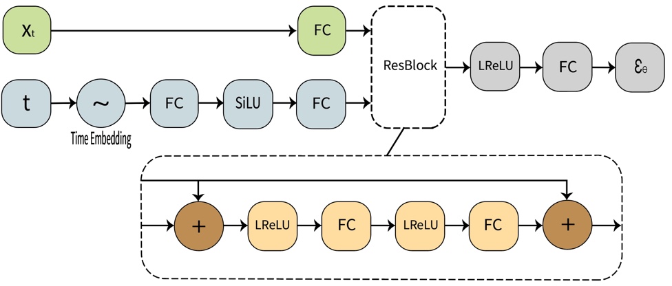
Figure 1: Proposed architecture for anomaly detection on tabular data. The model receives noisy sample $\bm{x}_{t}$ and time step $t$ that are fed forward to the ResBlock. The output of the ResBlock propagates through the Leaky-ReLU activation function followed by the FC layer to create the noise estimation of the real noise component in $\mathbf{x}_{t}$.

4 Experiments

Datasets.

We use 32 anomaly detection datasets from the ADBench repository [16] in this study (Appx. Tab. 5). Of these, 28 are real-world datasets, and the rest are extracted data-embedding representations of pre-trained models from the fields of computer vision (CV) and natural language processing (NLP). Specifically, the CV datasets include FashionMNIST and SVHN, for which both BERT and RoBERTa versions are utilized, and we randomly select the first class (out of 10 existing) for testing. The NLP datasets include Amazon and Yelp, and both ViT and ResNet versions are employed. In addition, due to convergence failure in some of the baselines, we stratified truncate Census to $50K$ samples, i.e., we maintain the original anomaly ratio post truncation.

Baseline methods and hyperparameters Settings.

We evaluate TabADM against eleven outlier detectors. Among them, nine are leading detectors from ADBench [16] with a wide variety and two recent NN based methods. The competitors from ADBench are $k$ Nearest Neighbors (KNN) [33], Local Outlier Factor (LOF) [8], One-Class Support Vector Machines (OCSVM) [38], PCA-based Outlier Detector (PCA) [40], Clustring-based Local Outlier Factor (CBLOF) [18], Isolation Forest (IForest) [29], Copula Based Outlier Detector (COPOD) [26], Histogram-based Outlier Detector (HBOS) [13] and Empirical Cumulative Distribution-based Outlier Detector (ECOD) [25]. We use PyOD [47] anomaly detection python package for implementation of baseline methods and use their default PyOD configuration for a fair comparison. Additionally, we include GOAD by Bergman et al. [6] and NeuTraL AD (referred to as NeuTraL) by Qiu et al. [32]. These methods have recently demonstrated impressive results on tabular data. We adopt the kdd based configuration for both methods for all experiments. The default hyperparameters we use for the training of TabADM are summarized in Appx. Tab. 4.

Results

We use the Area Under Receiver Operating Characteristic Curve (AUCROC) and Average Precision (AP) as evaluation metrics. We use a MacBook Pro laptop with M1, 16 GB of memory, and without GPU for all experimental runs.

In the first part, we follow the ADBench [16] experiment settings and use random stratified sampling to divide the data into 70% for training and 30% for testing. We repeat this process five times and report the average scores. In addition, to evaluate the performance of our method in high-dimensional data, we sort the 32 datasets in ascending order according to their dimensions and define the parameter $\tau$ as the percentile value corresponding to the dimensions. For each value of $\tau$, we partition the datasets into subgroups based on $\tau$, where each subgroup consists of datasets with dimensions greater than $\tau$. For example, when $\tau=10$, we form a group comprising the top 90% datasets with the highest number of variables. We calculate the average AUCROC and AP ranks for each sub-group for each method. We plot the values of the average ranks of both AUCROC and AP as a function of $\tau$.

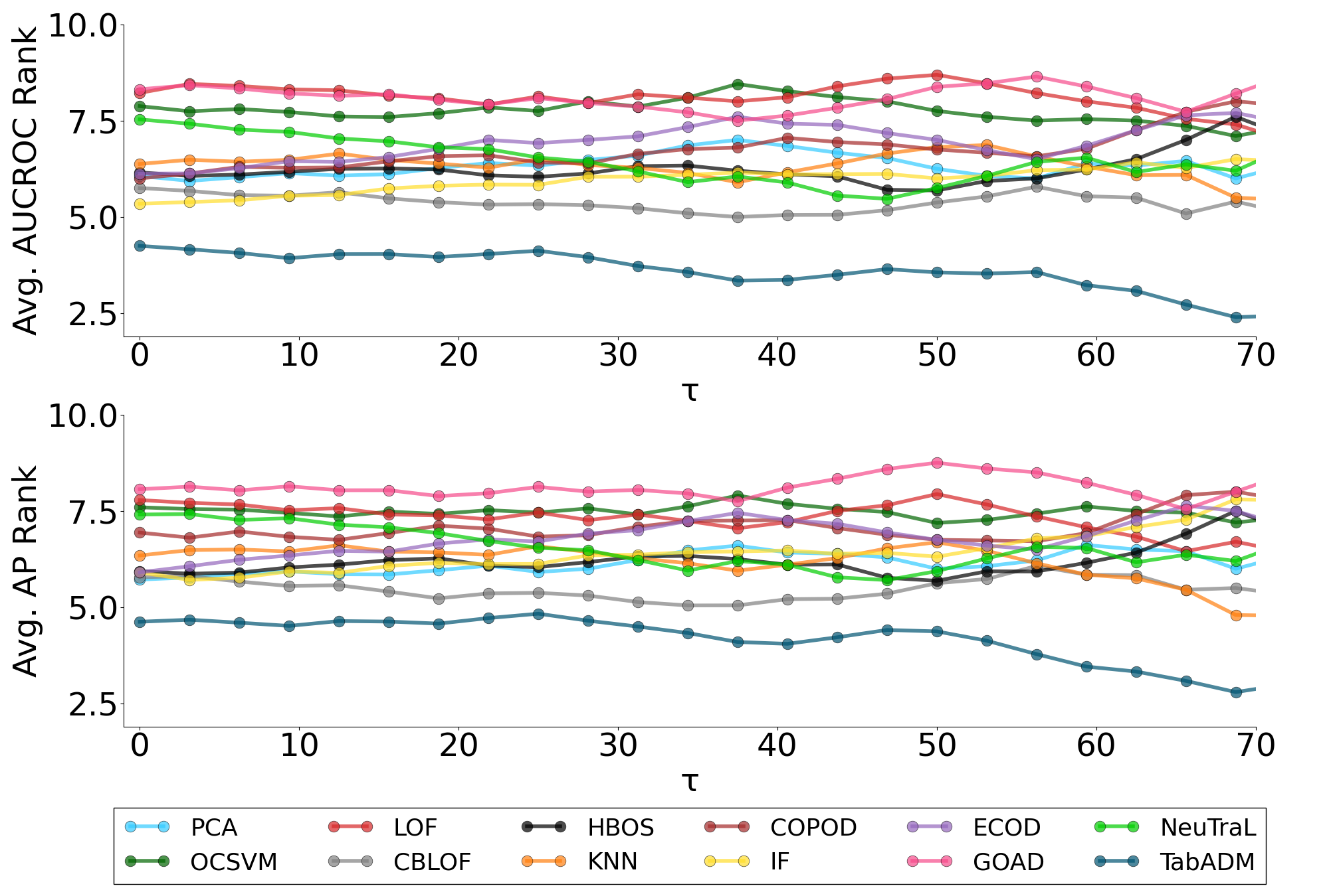
Figure 2: Average AUCROC (top) and AP (bottom) rank per method as a function of $\tau$, where $\tau$ is the percentile value corresponding to the number of dimensions. For example, when $\tau=10$, we form a subgroup comprising the top 90% of datasets with the highest number of variables and present the average ranks on this subgroup. We limit $\tau$ to a maximum of 70 to avoid an evaluation on a small subset of datasets.

The results for this part are presented in Tab. 1 and 2. The results of our proposed TabADM method demonstrate that, on average, it outperforms the other baselines in both AUCROC and AP scores, as well as in average rank, by a significant margin. Additionally, we observe that among the top 10 datasets with the highest dimensionality, TabADM achieves the highest AUCROC (AP) score in 5 (4) datasets. In light of this, we conduct a more in-depth analysis to evaluate the performance of the methods with respect to the dimensionality of the dataset. As illustrated in Fig. 2, TabADM demonstrates consistently low average ranks across all percentile values in both AUCROC and AP scores. Additionally, it can be observed that as the percentile value increases, the performance of TabADM improves, and the gap to the rest grows. This suggests that our model is particularly well-suited for large datasets.

Table 1: AUCROC scores for ADBench datasets.

Dataset	PCA	OCSVM	LOF	CBLOF	HBOS	KNN	COPOD	IF	ECOD	GOAD	NeuTraL	TabADM
Smtp	81.01	74.94	93.07	83.82	81.48	90.61	90.95	89.19	87.30	87.61	79.15	86.21
Mammogra.	87.05	83.72	73.15	80.15	83.91	82.69	89.00	84.56	88.96	57.27	52.89	82.79
Thyroid	96.04	87.58	86.37	94.10	95.91	95.49	94.07	97.73	97.84	73.19	92.20	93.84
Glass	74.52	55.27	66.02	85.59	83.23	88.39	78.06	80.65	76.02	64.41	49.25	88.71
Shuttle	98.95	98.15	53.59	75.59	98.68	63.40	99.41	99.72	99.27	98.56	95.11	98.97
Donors	82.85	73.11	61.65	65.36	71.88	62.68	81.41	77.76	88.80	30.90	50.26	72.48
PageBlocks	90.59	89.30	72.67	87.37	81.14	81.42	87.74	89.26	91.55	80.24	83.98	90.83
Vowels	62.54	58.31	94.76	90.69	68.74	98.23	52.45	79.17	61.43	93.46	45.94	96.80
Pendigits	92.61	92.62	51.44	90.26	92.20	72.97	88.99	94.77	91.60	63.17	86.04	86.20
Hepatitis	79.05	67.86	79.52	73.81	79.76	71.90	82.38	74.29	75.48	69.05	55.75	71.43
Cardio	94.27	91.96	64.08	80.27	83.34	72.17	91.16	90.91	92.90	59.40	26.30	81.70
Cardiotocogr.	75.82	79.19	58.43	65.97	60.51	54.63	66.80	68.85	79.13	39.79	77.29	60.97
Waveform	62.08	51.86	70.51	71.39	67.84	72.21	71.94	69.17	59.38	70.80	66.16	71.40
Letter	53.31	51.33	87.43	76.28	61.43	87.77	55.03	63.19	56.82	80.55	23.06	91.04
Ionosphere	79.03	74.42	85.93	89.52	65.65	92.43	79.54	84.43	73.66	87.49	83.41	92.67
Landsat	36.63	36.62	55.94	62.05	57.01	59.00	42.50	49.49	37.09	59.11	64.16	58.61
Satellite	60.34	59.97	55.17	72.97	75.27	65.53	63.47	71.38	58.51	64.90	77.25	72.53
Satimage-2	97.41	97.13	49.86	99.87	97.66	92.92	97.18	99.21	96.14	97.47	99.94	99.31
Celeba	78.58	69.70	42.49	60.19	75.63	57.46	75.17	69.91	75.81	26.69	70.79	69.05
SpamBase	56.36	54.96	45.14	57.78	65.69	54.82	69.11	61.37	66.00	38.26	40.02	58.93
Campaign	73.80	66.77	56.57	65.85	79.61	72.40	78.74	71.12	77.51	41.93	74.77	72.36
Optdigits	49.97	52.84	53.05	73.28	80.34	38.92	66.71	69.23	58.93	69.49	58.32	59.23
MNIST	85.35	82.69	68.30	79.67	61.94	81.42	77.92	80.47	75.10	83.58	88.49	86.13
Musk	100.00	81.19	37.80	100.00	100.00	70.93	94.71	99.97	95.58	100.00	76.15	100.00
Backdoor	88.68	84.77	71.57	83.10	75.66	68.20	78.91	73.22	84.56	90.48	89.99	91.83
Speech	51.39	50.99	53.99	51.17	51.92	52.26	53.13	53.50	51.46	46.74	40.19	54.54
Census	65.58	52.77	48.05	58.85	62.75	64.12	66.62	60.77	65.41	53.62	50.03	64.99
FashionM.	86.87	85.67	63.75	88.32	82.94	84.87	84.09	85.44	85.23	72.89	86.59	89.43
SVHN	55.57	55.86	65.79	59.70	51.03	62.51	51.50	55.97	53.09	58.93	64.10	62.75
Amazon	52.61	52.87	55.39	53.33	53.14	56.32	52.31	52.92	52.32	50.36	54.57	54.71
Yelp	56.09	56.30	61.94	60.12	56.44	62.71	55.33	56.93	55.60	50.36	59.58	58.77
InternetAds	60.24	68.75	64.77	68.41	68.28	70.10	67.51	67.90	67.57	41.82	46.10	76.48
AVG	73.91	69.98	64.01	75.15	74.09	71.92	74.49	75.70	74.25	65.70	65.87	77.99
AVG Rank	6.06	7.88	8.22	5.75	6.16	6.38	6.00	5.34	6.13	8.31	7.53	4.25

Table 2: AP scores for ADBench datasets.

Dataset	PCA	OCSVM	LOF	CBLOF	HBOS	KNN	COPOD	IF	ECOD	GOAD	NeuTraL	TabADM
Smtp	44.75	5.35	1.43	44.42	8.70	48.38	0.46	0.44	62.09	41.92	31.36	46.10
Mammogra.	19.93	11.84	10.33	7.96	19.35	16.10	40.23	19.50	40.67	5.84	3.04	15.68
Thyroid	42.26	19.49	16.87	26.16	52.55	29.88	19.41	60.16	49.60	35.65	34.44	31.19
Glass	20.65	16.81	22.53	25.28	25.42	26.82	18.97	21.59	25.68	16.67	7.80	39.06
Shuttle	90.35	94.69	9.68	40.51	95.07	16.42	95.56	97.92	89.81	85.60	52.89	92.52
Donors	16.68	10.42	10.50	8.25	12.24	10.64	20.76	13.07	26.33	5.13	5.58	11.59
PageBlocks	52.82	51.88	35.77	56.64	35.34	45.44	37.42	45.78	52.34	46.15	29.95	57.27
Vowels	8.54	9.19	43.12	23.99	11.64	67.26	4.05	15.79	10.46	39.49	5.28	64.12
Pendigits	19.86	19.51	3.88	16.37	24.16	6.23	16.54	28.71	25.19	5.92	14.95	9.83
Hepatitis	50.94	28.67	37.08	31.76	43.31	29.73	50.84	34.82	36.97	33.23	22.54	32.30
Cardio	57.18	53.33	18.25	36.56	42.68	31.25	52.56	48.48	53.55	29.43	7.95	31.77
Cardiotocogr.	48.48	54.43	30.42	44.03	39.37	33.88	40.78	43.03	51.65	24.40	61.81	37.07
Waveform	4.80	3.94	9.22	15.11	5.08	10.77	5.67	6.21	4.47	44.14	5.32	6.26
Letter	10.16	8.62	43.76	19.55	10.32	34.73	7.36	9.91	8.63	30.47	4.25	49.66
Ionosphere	73.13	72.76	81.22	87.74	46.00	92.36	68.86	79.49	65.74	85.59	75.54	92.37
Landsat	16.43	16.33	26.49	29.36	23.26	25.95	17.89	20.12	16.61	24.89	26.72	24.95
Satellite	60.80	58.98	38.45	62.19	67.70	50.55	57.18	66.20	52.65	43.94	72.87	56.15
Satimage-2	87.19	86.03	3.37	97.32	80.89	34.83	79.94	91.31	68.14	43.72	96.35	62.75
Celeba	11.28	7.41	1.78	3.30	9.77	2.69	9.63	7.08	9.86	1.39	4.62	4.37
SpamBase	42.21	41.59	35.91	43.27	50.36	42.70	54.74	50.14	52.21	34.74	35.71	43.69
Campaign	28.97	28.58	12.12	21.12	37.45	26.43	37.01	30.23	35.57	10.46	31.10	29.52
Optdigits	2.67	2.90	5.00	4.99	11.01	2.54	4.21	5.19	3.40	5.01	3.70	4.22
MNIST	39.63	32.97	22.73	30.91	13.41	38.31	22.37	28.43	18.27	38.35	41.96	44.17
Musk	100.00	10.47	3.57	100.00	100.00	10.78	35.61	99.80	48.73	100.00	6.98	100.00
Backdoor	52.13	8.62	20.69	7.19	5.47	30.55	6.92	3.91	9.25	55.48	36.38	41.29
Speech	2.98	3.07	3.90	3.08	3.19	3.37	3.03	2.84	3.28	2.38	1.48	3.99
Census	8.76	6.27	5.51	6.94	7.88	8.16	8.98	7.33	8.58	6.54	5.78	8.51
FashionM.	26.42	24.90	11.27	28.40	23.65	23.96	24.21	23.04	24.84	17.74	31.89	37.82
SVHN	7.03	7.02	9.83	8.12	6.00	8.81	6.16	7.04	6.31	7.84	8.94	8.49
Amazon	5.43	5.44	5.69	5.48	5.48	5.79	5.40	5.49	5.35	5.26	5.63	5.60
Yelp	6.01	6.11	7.56	6.50	6.15	7.57	6.04	6.17	5.84	5.01	6.85	6.55
InternetAds	27.54	53.29	37.81	53.15	52.33	41.63	50.35	50.04	50.46	53.05	17.89	53.05
AVG	33.94	26.90	19.55	31.11	30.48	27.02	28.41	32.16	31.95	29.70	24.92	36.00
AVG Rank	5.72	7.59	7.78	5.78	5.94	6.34	6.94	5.91	5.91	8.06	7.41	4.63

In the second part, we randomly divide Satellite, Cardiotocography, and SpamBase datasets into training and test sets using a 70-30 split. Then, we create 11 sub-training sets with varying contamination ratios from 0% to 10%. In addition, we randomly fix a 10% contamination ratio in the test set. We repeat this process 5 times and plot the average AUCROC and AP scores as a function of contamination ratios for each dataset.

The results in this part are shown in Fig. 3. As the level of contamination in the training set increases, there is a decline in both the AUCROC and AP scores. This can be attributed to the fact that the model learns the anomalous samples in addition to the inlier samples. As a result, the ability of our model to accurately distinguish between inliers and outliers is hindered, leading to a decrease in performance.

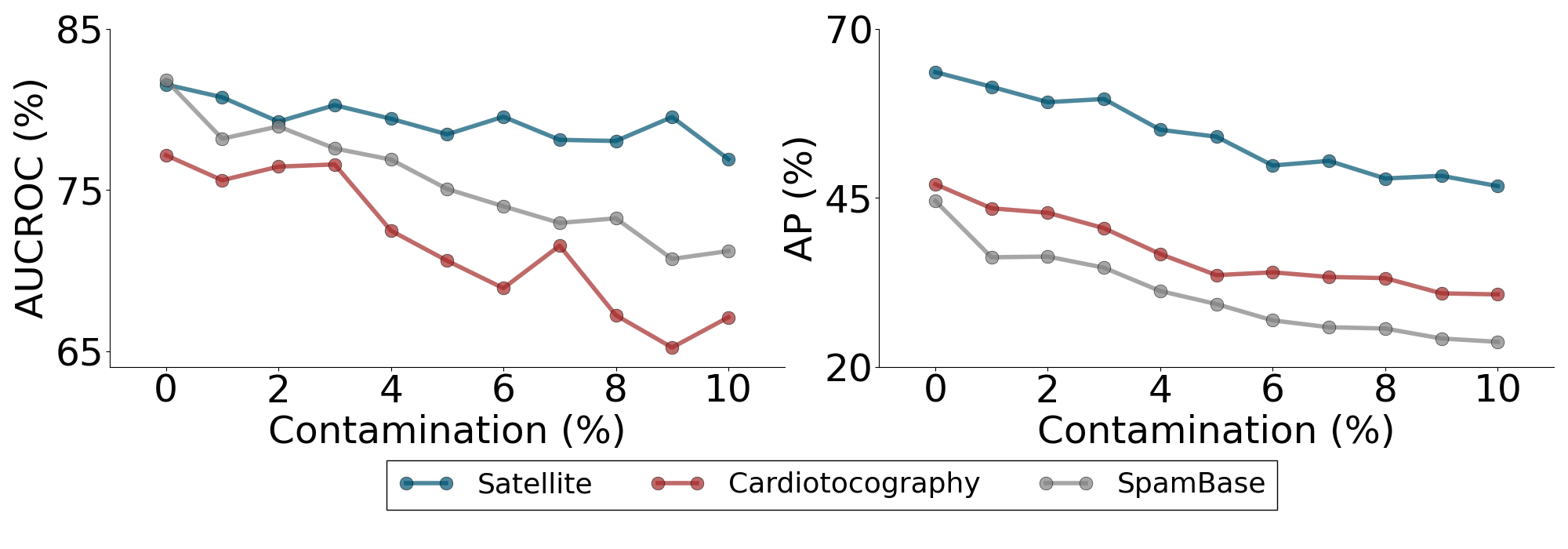
Figure 3: AUCROC (left) and AP (right) scores for the Satellite, Cardiotocography, and SpamBase datasets decrease as the contamination percentage increases. This is due to the increasing influence of anomalous samples on the overall probability distribution learned by the model.

In the third part, we investigate the impact of different training hyperparameters on the performance of our model. We examine the relationship between the AUCROC and AP scores and the number of training iterations for Landsat, Letter, and Musk. In addition, we investigate the influence of the number of rejections samples (m) on the performance. As in previous parts, we use a 70-30 train-test random split over five times and report the average AUCROC and AP scores for $m=0,1,4,7$.

Fig. 4 and Tab. 3 present the results for this part. As shown in Fig. 4, as the number of training steps increases, the performance of all datasets improves. However, the improvement rate varies among different datasets. Tab. 3 demonstrates that excluding the sample with the highest loss in a batch during training ($m=1$) leads to the highest average scores. This indicates that the model is more robust to anomalies, resulting in better modeling of the normal underlying distribution and, consequently, improved overall performance.

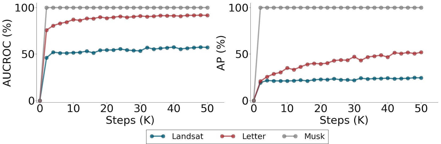
Figure 4: AUCROC (left) and AP (right) scores for the Landsat, Letter, and Mask datasets as functions of training steps.

Table 3: Comparison of AUCROC (left) and AP (right) scores for the Landset, Letter and Musk datasets for different values of rejection samples $m$ from batch of size 8.

	AUCROC (%)				AP (%)
Dataset	m=0	m=1	m=4	m=7	m=0	m=1	m=4	m=7
Landsat	56.78	58.61	55.78	54.88	24.41	24.95	22.73	22.67
Letter	91.28	91.04	90.75	81.06	48.24	49.66	39.81	22.00
Musk	99.10	100.00	100.00	100.00	72.56	100.00	100.00	100.00

5 Conclusion and Future Work

In this paper, we introduce a novel unsupervised outlier detection method, TabADM, which utilizes the diffusion models technique to estimate the probability distribution of the data. It then assigns outlier scores to unseen samples based on their probability of being generated from the model. In addition, a rejection scheme is introduced to enhance performance when outliers are present in the data. TabADM exhibits strong training stability and alleviates the need for hyperparameter tuning. Furthermore, it demonstrates exceptional performance in high-dimensional datasets, surpassing other SOTA methods.

TabADM has certain drawbacks, including long training and inference times compared to other methods and a lack of interpretability. Future work could focus on improving these drawbacks. For example, the inference time can be reduced by decreasing the number of diffusion steps used per sample, although this may impact performance. Additionally, efforts could be made to enhance interpretability. This could be achieved through simple measures such as identifying which features contribute most significantly to the total loss, as well as more complex measures such as identifying common feature patterns in the data that may serve as indicators for abnormality. Another possible future research direction would be to extend the capabilities of TabADM such as enabling it to handle missing feature values.

Appendix

Appendix A Defualt hyperparameters

Tab. 4 presents the default hyperparameters employed for the training procedure in our experiments. While most hyperparameters remain constant, the learning rate and the size of the fully connected (FC) layers are determined by the number of dimensions ($d$) of the training dataset.

Table 4: Default hyperparameters for TabADM training procedure.

# Dims. in dataset (d)	$d\leq 100$	$100<d\leq 1000$	$1000<d\leq 2000$
FC layers size	512	1024	2048
Learning rate	$1X10^{-3}$	$2X10^{-4}$	$2X10^{-4}$
Weight decay	$1X10^{-4}$	$1X10^{-4}$	$1X10^{-4}$
Time embedding size	64	64	64
Batch size (k)	8	8	8
Rejection samples (m)	1	1	1
Train steps (e)	50K	50K	50K
Noise schedule	linear	linear	linear
Diffusion timesteps (T)	100	100	100
Loss type	Simplified MSE of $\epsilon$	Simplified MSE of $\epsilon$	Simplified MSE of $\epsilon$

Appendix B Evaluation datasets

Tab. 5 lists the ADBench [16] datasets used for evaluation. To ensure a fair comparison between the baselines, we selected diverse datasets in terms of their dimensions ($d$), number of samples ($n$), and anomaly rates.

The list contains 32 datasets. Among them, 28 real-world tabular datasets and the other 4 are extracted feature embedding representations of pre-trained models from CV and NLP fields. The CV datasets include FashionMNIST and SVHN, and we randomly selected the first class (out of 10 classes) for testing. In addition, each dataset has two versions: the features of the first version are based on a pre-trained ResNet model with 512 dimensions, while the features of the second version are based on a pre-trained ViT model with 1000 dimensions. Similarly, the NLP datasets include Amazon and Yelp, each with two versions. One is based on a pre-trained BERT model, and the other is based on a pre-trained RoBERTa model. Both versions have 768 dimensions. For the CV and NLP datasets, we reported the average AUCROC and AP scores across the two versions. Lastly, due to convergence failure in some of the baselines, we randomly sub-sampled Census to 50,000 samples in a stratified way to preserve the original anomaly rate post-truncation.

Table 5: List of ADBench datasets used for evaluation.

Dataset	# Dims. ($d$)	# Samp. ($n$)	Anomaly rate (%)
Smtp	3	95156	0.03
Mammography	6	11183	2.32
Thyroid	6	3772	2.47
Glass	7	214	4.21
Shuttle	9	49097	7.15
Donors	10	619326	5.93
PageBlocks	10	5393	9.46
Vowels	12	1456	3.43
Pendigits	16	6870	2.27
Hepatitis	19	80	16.25
Cardio	21	1831	9.61
Cardiotocography	21	2114	22.04
Waveform	21	3443	2.90
Letter	32	1600	6.25
Ionosphere	33	351	35.90
Landsat	36	6435	20.71
Satellite	36	6435	31.64
Satimage-2	36	5803	1.22
Celeba	39	202599	2.24
SpamBase	57	4207	39.91
Campaign	62	41188	11.27
Optdigits	64	5216	2.88
MNIST	100	7603	9.21
Musk	166	3062	3.17
Backdoor	196	95329	2.44
Speech	400	3686	1.65
Census	500	50000	6.20
FashionMNIST	512/1000	6315	5.00
SVHN	512/1000	5208	5.00
Amazon	768/768	10000	5.00
Yelp	768/768	5000	5.00
InternetAds	1555	1966	18.72

References

- [1] C. C. Aggarwal, A. Hinneburg, and D. A. Keim. On the Surprising Behavior of Distance Metrics in High Dimensional Space. In Database Theory — ICDT 2001, pages 420–434, 2001.
- [2] C. C. Aggarwal and P. S. Yu. Outlier Detection for High Dimensional Data. In Proceedings of the 2001 ACM SIGMOD international conference on Management of data, pages 37–46, 2001.
- [3] J. An and S. Cho. Variational Autoencoder based Anomaly Detection using Reconstruction Probability. Special lecture on IE, 2(1):1–18, 2015.
- [4] Y. Balaji, S. Nah, X. Huang, A. Vahdat, J. Song, Q. Zhang, K. Kreis, M. Aittala, T. Aila, S. Laine, B. Catanzaro, T. Karras, and M.-Y. Liu. eDiff-I: Text-to-Image Diffusion Models with an Ensemble of Expert Denoisers, 2023. arXiv:2211.01324.
- [5] D. Baranchuk, I. Rubachev, A. Voynov, V. Khrulkov, and A. Babenko. Label-Efficient Semantic Segmentation With Diffusion Models. In ICLR, 2022.
- [6] L. Bergman and Y. Hoshen. Classification-Based Anomaly Detection for General Data. In ICLR, 2020.
- [7] Y Bregman, O Lindenbaum, and N Rabin. Array based earthquakes-explosion discrimination using diffusion maps. Pure and Applied Geophysics, 178:2403–2418, 2021.
- [8] M. M. Breunig, H.-P. Kriegel, R. T. Ng, and J. Sander. LOF: Identifying Density-Based Local Outliers. SIGMOD Rec., 29(2):93–104, 2000.
- [9] B. Cao, M. Mao, S. Viidu, and P. Yu. Collective Fraud Detection Capturing Inter-Transaction Dependency. In Proceedings of the KDD 2017: Workshop on Anomaly Detection in Finance, volume 71, pages 66–75, 2018.
- [10] N. Chen, Y. Zhang, H. Zen, R. J. Weiss, M. Norouzi, and W. Chan. WaveGrad: Estimating Gradients for Waveform Generation. In ICLR, 2021.
- [11] L. Deecke, R. Vandermeulen, L. Ruff, S. Mandt, and M. Kloft. Anomaly Detection with Generative Adversarial Networks, 2018.
- [12] P. Dhariwal and A. Nichol. Diffusion Models Beat GANs on Image Synthesis. In NeurIPS, volume 34, pages 8780–8794, 2021.
- [13] M. Goldstein and A. Dengel. Histogram-Based Outlier Score (HBOS): A fast Unsupervised Anomaly Detection Algorithm. KI: Poster and Demo Track, 09 2012.
- [14] Y. Gorishniy, I. Rubachev, V. Khrulkov, and A. Babenko. Revisiting Deep Learning Models for Tabular Data. In NeurIPS, 2021.
- [15] F. E. Grubbs. Procedures for Detecting Outlying Observations in Samples. Technometrics, 11(1):1–21, 1969.
- [16] S. Han, X. Hu, H. Huang, M. Jiang, and Y. Zhao. ADBench: Anomaly Detection Benchmark. In NeurIPS, 2022.
- [17] Z. He, S. Deng, and X. Xu. A Unified Subspace Outlier Ensemble Framework for Outlier Detection. In Advances in Web-Age Information Management, pages 632–637, 2005.
- [18] Z. He, X. Xu, and S. Deng. Discovering Cluster-Based Local Outliers. Pattern Recognition Letters, 24(9):1641–1650, 2003.
- [19] J. Ho, A. Jain, and P. Abbeel. Denoising Diffusion Probabilistic Models. In NeurIPS, volume 33, pages 6840–6851, 2020.
- [20] J. Ho, T. Salimans, A. Gritsenko, W. Chan, M. Norouzi, and D. J. Fleet. Video Diffusion Models. In NeurIPS, volume 35, pages 8633–8646, 2022.
- [21] J. Hollmén and V. Tresp. Call-Based Fraud Detection in Mobile Communication Networks Using a Hierarchical Regime-Switching Model. In NIPS, volume 11, 1998.
- [22] Lina Irshaid, Jonathan Bleiberg, Ethan Weinberger, James Garritano, Rory M Shallis, Jonathan Patsenker, Ofir Lindenbaum, Yuval Kluger, Samuel G Katz, and Mina L Xu. Histopathologic and machine deep learning criteria to predict lymphoma transformation in bone marrow biopsies. Archives of Pathology & Laboratory Medicine, 146(2):182–193, 2022.
- [23] J. Laurikkala and M. Juhola and E. Kentala. Informal Identification of Outliers in Medical Data. In Workshop Notes of the 14th European Conference on Artificial Intelligence (ECAI-2000): The Fifth Workshop on Intelligent Data Analysis in Medicine and Pharmacology (IDAMAP-2000), pages 20–24, 2000.
- [24] C. Kruegel, D. Mutz, W. Robertson, and F. Valeur. Bayesian event classification for intrusion detection. In 19th Annual Computer Security Applications Conference, pages 14–23, 2003.
- [25] Z. Li, X. Hu Y. Zhao, N. Botta, C. Ionescu, and G. H. Chen. ECOD: Unsupervised Outlier Detection Using Empirical Cumulative Distribution Functions. IEEE Transactions on Knowledge and Data Engineering (TKDE), pages 1–1, 2022.
- [26] Z. Li, Y. Zhao, N. Botta, C. Ionescu, and X. Hu. COPOD: Copula-Based Outlier Detection. In 2020 IEEE International Conference on Data Mining (ICDM), pages 1118–1123, 2020.
- [27] Ofir Lindenbaum, Yariv Aizenbud, and Yuval Kluger. Probabilistic robust autoencoders for outlier detection. arXiv preprint arXiv:2110.00494, 2021.
- [28] Ofir Lindenbaum, Neta Rabin, Yuri Bregman, and Amir Averbuch. Multi-channel fusion for seismic event detection and classification. In 2016 IEEE International Conference on the Science of Electrical Engineering (ICSEE), pages 1–5. IEEE, 2016.
- [29] F. T. Liu, K. M. Ting, and Z.-H. Zhou. Isolation Forest. In 2008 IEEE International Conference on Data Mining (ICDM), pages 413–422, 2008.
- [30] Y. Liu, Z. Li, C. Zhou, Y. Jiang, J. Sun, M. Wang, and X. He. Generative adversarial active learning for unsupervised outlier detection. TKDE, 32(8):1517–1528, 2019.
- [31] C. Qiu, A. Li, M. Kloft, M. Rudolph, and S. Mandt. Latent Outlier Exposure for Anomaly Detection with Contaminated Data. In ICML, pages 18153–18167, 2022.
- [32] C. Qiu, T. Pfrommer, M. Kloft, S. Mandt, and M. Rudolph. Neural Transformation Learning for Deep Anomaly Detection Beyond Images. In ICML, pages 8703–8714, 2021.
- [33] S. Ramaswamy, R. Rastogi, and K. Shim. Efficient algorithms for mining outliers from large data sets. SIGMOD Rec., 2000.
- [34] Amit Rozner, Barak Battash, Henry Li, Lior Wolf, and Ofir Lindenbaum. Anomaly detection with variance stabilized density estimation. arXiv preprint arXiv:2306.00582, 2023.
- [35] C. Saharia, W. Chan, S. Saxena, L. Li, J. Whang, E. L. Denton, K. Ghasemipour, R. Gontijo Lopes, B. Karagol Ayan, T. Salimans, J. Ho, D. J. Fleet, and M. Norouzi. Photorealistic Text-to-Image Diffusion Models with Deep Language Understanding. In NeurIPS, volume 35, pages 36479–36494, 2022.
- [36] D. Savage, X. Zhang, X. Yu, P. Chou, and Q. Wang. Anomaly Detection in Online Social Networks. Social Networks, 39:62–70, 2014.
- [37] T. Schlegl, P. Seeböck, S. M Waldstein, U. Schmidt-Erfurth, and G. Langs. Unsupervised anomaly detection with generative adversarial networks to guide marker discovery. In Information Processing in Medical Imaging: 25th International Conference, pages 146–157, 2017.
- [38] B. Schölkopf, R. C. Williamson, A. Smola, J. Shawe-Tailor, and J. Platt. Support Vector Method for Novelty Detection. In NIPS, volume 12, 1999.
- [39] K. Sequeira and M. Zaki. ADMIT: Anomaly-Based Data Mining for Intrusions. In Proceedings of the Eighth ACM SIGKDD International Conference on Knowledge Discovery and Data Mining, pages 386–395, 2002.
- [40] M.-L. Shyu, S.-C. Chen, K. Sarinnapakorn, and L. Chang. A Novel Anomaly Detection Scheme Based on Principal Component Classifier. Technical report, Miami Univ Coral Gables Fl Dept of Electrical and Computer Engineering, 2003.
- [41] A. O. Tur, N. Dall’Asen, C. Beyan, and E. Ricci. Exploring Diffusion Models for Unsupervised Video Anomaly Detection, 2023. arXiv:2304.05841.
- [42] A. Vaswani, N. Shazeer, N. Parmar, J. Uszkoreit, L. Jones, A. N. Gomez, L. Kaiser, and I. Polosukhin. Attention Is All You Need. In NIPS, volume 30, 2017.
- [43] J. Wolleb, F. Bieder, R. Sandkühler, and P. C. Cattin. Diffusion Models for Medical Anomaly Detection. In Medical Image Computing and Computer Assisted Intervention–MICCAI 2022: 25th International Conference, pages 35–45, 2022.
- [44] J. Wolleb, R. Sandkühler, F. Bieder, P. Valmaggia, and P. C. Cattin. Diffusion Models for Implicit Image Segmentation Ensembles. In International Conference on Medical Imaging with Deep Learning, pages 1336–1348, 2022.
- [45] J. Wyatt, A. Leach, S. M. Schmon, and C. G. Willcocks. AnoDDPM: Anomaly Detection with Denoising Diffusion Probabilistic Models using Simplex Noise. In 2022 IEEE/CVF Conference on Computer Vision and Pattern Recognition Workshops (CVPRW), pages 649–655, 2022.
- [46] X. Yang, L. Latecki, and D. Pokrajac. Outlier Detection with Globally Optimal Exemplar-Based GMM. SIAM, pages 145–154, 2009.
- [47] Y. Zhao, Z. Nasrullah, and Z. Li. PyOD: A Python Toolbox for Scalable Outlier Detection. JMLR, 20(96):1–7, 2019.
- [48] C. Zhou and R. C. Paffenroth. Anomaly Detection with Robust Deep Autoencoders. In Proceedings of the 23rd ACM SIGKDD International Conference on Knowledge Discovery and Data Mining, pages 665–674, 2017.
- [49] B. Zong, Q. Song, M. R. Min, W. Cheng, C. Lumezanu, D. Cho, and H. Chen. Deep Autoencoding Gaussian Mixture Model for Unsupervised Anomaly Detection. In ICLR, 2018.