Green’s Function Zeros in Fermi Surface Symmetric Mass Generation
Abstract
The Fermi surface symmetric mass generation (SMG) is an intrinsically interaction-driven mechanism that opens an excitation gap on the Fermi surface without invoking symmetry-breaking or topological order. We explore this phenomenon within a bilayer square lattice model of spin-1/2 fermions, where the system can be tuned from a metallic Fermi liquid phase to a strongly-interacting SMG insulator phase by an inter-layer spin-spin interaction. The SMG insulator preserves all symmetries and has no mean-field interpretation at the single-particle level. It is characterized by zeros in the fermion Green’s function, which encapsulate the same Fermi volume in momentum space as the original Fermi surface, a feature mandated by the Luttinger theorem. Utilizing both numerical and field-theoretical methods, we provide compelling evidence for these Green’s function zeros across both strong and weak coupling regimes of the SMG phase. Our findings highlight the robustness of the zero Fermi surface, which offers promising avenues for experimental identification of SMG insulators through spectroscopy experiments despite potential spectral broadening from noise or dissipation.
I Introduction
Symmetric mass generation (SMG) [1, 2, 3, 4, 5, 6, 7, 8] is an interaction-driven mechanism that creates many-body excitation gaps in anomaly-free fermion systems without condensing any fermion bilinear operator or developing topological orders. It has emerged as a alternative symmetry-preserving approach for mass generation in relativistic fermion systems, which is distinct from the traditional symmetry-breaking Higgs mechanism [9, 10, 11, 12, 13, 14]. The prospect of SMG offering a potential solution to the long-standing fermion doubling problem [15, 16, 17, 18, 19, 20, 21] has sparked significant interest in the lattice gauge theory community [22, 23, 24, 25, 26, 27, 28, 29, 30, 31, 32, 33, 34, 35, 36, 37, 38, 39, 40, 41, 42, 43, 44, 45, 46]. In condensed matter physics, SMG was initially explored within the framework of the interaction-reduced classification of fermionic symmetry protected topological (SPT) states [1, 2, 47, 48, 49, 50, 51, 52, 53, 54, 55, 56, 57, 58, 59, 60, 61, 62, 63, 64, 65, 66, 67, 68], and has been recently extended to systems with Fermi surfaces [69, 70, 71, 72, 73, 74], given the growing understanding that Fermi liquids can be perceived as fermionic SPT states within the phase space [75, 76].
One important feature of the SMG gapped state lies in the zeros of fermion Green’s function [77, 78, 79, 80, 81, 82] at low-energy. Investigations reveal that the poles of the fermion Green’s function in the pristine gapless fermion state will be replaced by zeros in the gapped SMG state as the fermion system goes across the SMG transition upon increasing the interaction strength. This pole-to-zero transition was postulated [78] as a direct indicator of the SMG transition [80, 83] that can be probed by spectroscopy experiments. However, the presence of similar zeros in the Green’s function within Fermi surface SMG states has not been investigated yet, and it is the focus of our present research.
Fermi surface SMG [74] refers to the occurrence of SMG phenomena on Fermi surfaces with non-zero Fermi volumes. It describes scenarios where the fermion interaction transforms a gapless Fermi liquid state (metal) into a non-degenerate, gapped, direct product state (trivial insulator), without breaking any symmetry (for example, without invoking Cooper pairing or density wave orders). Such a metal-insulator transition is viable when Fermi surfaces collaboratively cancel the Fermi surface anomaly [84, 85, 74]. This anomaly can be perceived as a mixed anomaly between the translation symmetry and the charge conservation symmetry on the lattice [86, 87, 88, 89, 85, 84, 90], or as an anomaly of an emergent loop symmetry [91, 92, 93] in the infrared theory.
In this work, we present evidence of robust Green’s function zeros in Fermi surface SMG states. Let be the energy scale of band dispersion and be the energy scale of SMG gapping interaction, we investigate the problem from two parameter regimes:
-
•
Deep in the SMG phase (), we start with an exact-solvable SMG product state in a lattice model and calculate the fermion Green’s function by treating the fermion hopping as perturbation [94]. We find that the Green’s function deep in the SMG phase takes the following form
(1) where labels the frequency-momentum of the the fermion. is the energy dispersion of the original band structure in the free-fermion limit, and is an order-one number depending on other details of the system. One salient feature of is that it has a series of zeros at in the frequency-momentum space. At , the Green’s function zeros form a zero Fermi surface that replaces the original Fermi surface.
-
•
If the SMG phase is adjacent to a spontaneous symmetry breaking (SSB) phase, we use perturbative field theory to argue that the Green’s function in the SMG phase near the symmetry-breaking transition () should take the form of
(2) where we assume that the SSB order parameter retains a finite amplitude in the SMG phase, but its phase is randomly fluctuating [95]. Again, features a series of zeros at , with the same zero Fermi surface.
Many previous works [96, 97, 98, 99] suggest that the Luttinger theorem [100] will not be violated in the presence of the interaction that preserves the translation and charge conservation symmetry. However, quasi-particles (poles of Green’s function) may not exist in the strongly correlated systems, the Fermi surface is instead defined by the surface of Green’s function zeros at zero frequency, i.e., , and the Green’s function changes sign on the two sides of the zero Fermi surface, or the so-called Luttinger surface [101, 98, 91, 102, 103]. This can be regarded as the remnant of the conventional Fermi surface in the strongly interacting gapped phase. Our analysis shows that the volume enclosed by the zeros of the Green’s function in the SMG phase is the same as the Fermi volume in the Fermi liquid phase, which agrees with the Luttinger theorem.
The paper will be structured as follows. We start by introducing a concrete lattice model for Fermi surface SMG in Sec. II.1 and briefly discussing its phase diagram. We give theoretical arguments for Green’s function zeros in the SMG phase from the Luttinger theorem in Sec. II.2 (general), and the particle-hole symmetry in Sec. II.3 (specific). We provide numerical and field theoretical evidence of Green’s function zeros from both the strong coupling Sec. III.1 and the weak coupling Sec. III.2 perspectives. We comment on the robustness of probing the zero structure in spectroscopy experiments in Sec. IV. We conclude in Sec. V with a discussion of the relevance of our model to the nickelate superconductor La3Ni2O7.
II Argument For Green’s Function Zeros
II.1 Lattice Model and Phase Diagram
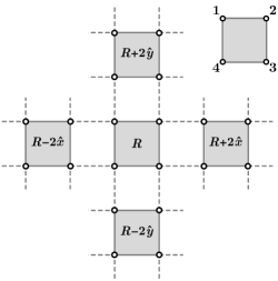
As a specific example of Fermi surface SMG, we consider a bilayer square lattice [104, 105, 106] model of spin-1/2 fermions, as illustrated in Fig. 1(a). Let be the fermion annihilation operator on site- layer- () and spin- (). The model is described by the following Hamiltonian
| (3) |
where denotes the spin operator with being the Pauli matrices. The Hamiltonian contains a nearest-neighbor hopping of the fermions within each layer and an inter-layer Heisenberg spin-spin interaction with antiferromagnetic coupling . The Heisenberg interaction should be understood as a four-fermion interaction, that there is no explicitly formed local moment degrees of freedom. Unlike the standard - model [107], we do not impose any on-site single-occupancy constraint [108] here. We assume that the fermions are half-filled in each layer.
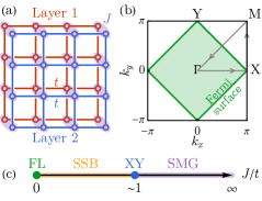
In the non-interacting limit (), the ground state of the tight-binding Hamiltonian in Eq. (3) is a Fermi liquid with a four-fold degenerated (two layers and two spins) square-shaped Fermi surface in the Brillouin zone, as shown in Fig. 1(b). The fermion system is gapless in this limit. However, given that the fermion carries one unit charge under the symmetry, the Fermi surface anomaly vanishes due to [87, 76]
| (4) |
where indexes the four-fold degenerated Fermi surface with being the charge carried by the fermion and being the filling fraction. This implies there must be a way to gap out the Fermi surface into a trivial insulator while preserving both the translation and the charge conservation symmetries. Nevertheless, these symmetry requirements are restrictive enough to rule out all possible fermion bilinear gapping mechanisms, leaving Fermi surface SMG the only available option.
One possible SMG gapping interaction is the interlayer Heisenberg spin-spin interaction in Eq. (3). In the strong interaction limit (), the system has a unique ground state, given by
| (5) |
which is a direct product of the inter-layer spin-singlet state on every site. stands for the vacuum state of fermions (i.e. ). The SMG ground state does not break any symmetry and does not have topological order. All excitations are gapped by an energy of the order from the ground state. Any local perturbation far below the energy scale can not close this excitation gap, so the SMG phase is expected to be stable in a large parameter regime as long as .
Given the distinct ground states in the two limits of , we anticipate at least one quantum phase transition separating the Fermi liquid and the SMG insulator. However, due to the perfect nesting of the Fermi surface, the Fermi liquid state is unstable towards spontaneous symmetry breaking (SSB) upon infinitesimal interaction, so a more plausible phase diagram should look like Fig. 1(c), where an intermediate SSB phase sets in. A mean-field analysis based on the Fermi liquid fixed point shows that there are two degenerated leading instabilities: (i) the inter-layer exciton condensation (EC) and (ii) the inter-layer superconductivity (SC). They are respectively described by the following order parameters
| (6) |
Here, denotes the stagger sign on the square lattice of lattice momentum . for and for . stands for the opposite spin of .
The energetic degeneracy of these two SSB orders can be explained by the fact that their order parameters and are related by a particle-hole transformation in the second layer only, which is a symmetry of the model Hamiltonian in Eq. (3). The EC spontaneously breaks the translation and interlayer symmetry, and the SC spontaneously breaks the total symmetry. Both of them gap out the Fermi surfaces fully, leading to an SSB insulator (or superconductor). The SSB and SMG phases are likely separated by an XY transition, at which the symmetry gets restored. We will leave the numerical verification of the proposed phase diagram Fig. 1(c) for future study, as the main focus of this research is to investigate the structure of fermion Green’s function in the SMG insulating phase.
We note that the model Eq. (3) was also introduced as the “coupled ancilla qubit” model to describe the pseudo-gap physics in the recent literature [70, 72, 73]. Its honeycomb lattice version has been investigated in recent numerical simulations [109], where a direct quantum phase transition between semimetal and insulator phases was observed.
II.2 Luttinger Theorem and Green’s Function Zeros
The Luttinger theorem [110, 100] asserts that in a fermion many-body system with lattice translation and charge symmetries, the ground state charge density (i.e., the charge per unit cell) is tied to the momentum space volume in which the real part of the zero-frequency fermion Green’s function is positive . This can be formally expressed as
| (7) |
Here, the symmetry generator measures the total charge, and the volume is defined as the number of unit cells in the lattice system. counts the fermion flavor number (or the Fermi surface degeneracy), including two layers and two spins. The Green’s function in Eq. (7) is defined by the fermion two-point correlation as
| (8) |
The correlation function is proportional to an identity matrix in the flavor (layer-spin) space because of the layer , the layer interchange , and the spin symmetries.
The Luttinger theorem applies to the Fermi liquid and SMG states in the bilayer square lattice model Eq. (3), as both states preserve the translation and charge symmetries. Given that the fermions are half-filled () in the system, the Fermi volume should be
| (9) |
The Fermi volume is enclosed by the Fermi surface, across which changes sign. The sign change can be achieved either by poles or zeros in the Green’s function.
In the Fermi liquid state, the required Fermi volume is satisfied via Green’s function poles along the Fermi surface, as pictured in Fig. 1(b). However, the SMG insulator is a fully gapped state of fermions that has no low-energy quasi-particles (below the energy scale ). Consequently, the Green’s function cannot develop poles at , meaning the required Fermi volume can only be satisfied by Green’s function zeros. Therefore, the Lutinger theorem implies that there must be robust Green’s function zeros at low energy in the SMG phase, and the zero Fermi surface must enclose half of the Brillouin zone volume in place of the original pole Fermi surface.
II.3 Particle-Hole Symmetry and Zero Fermi Surface
The Luttinger theorem only constrains the Fermi volume but does not impose requirements on the shape of the Fermi surface. However, in this particular example of the bilayer square lattice model Eq. (3), the system has sufficient symmetries to determine even the shape of the Fermi surface.
The key symmetry here is a particle-hole symmetry , which acts as
| (10) |
The Hamiltonian in Eq. (3) is invariant under this transformation. Since the Green’s function is an identity matrix in the flavor space Eq. (8) which is invariant under any flavor basis transformation, we can omit the flavor indices and focus on the frequency-momentum dependence of the Green’s function, written as
| (11) |
Given Eq. (10), the fermion field transforms under the symmetry as
| (12) |
where is the momentum associated with the stagger sign factor on the square lattice. As a consequence, the Green’s function transforms as
| (13) |
Furthermore, there are also two diagonal reflection symmetries on the square lattice, which maps to or in the momentum space.
Both the Fermi liquid and the SMG states preserve the particle-hole symmetry and the lattice reflection symmetry, which requires the Green’s function to be invariant under the combined symmetry transformations. So the zero-frequency Green’s function must satisfy
| (14) |
meaning that the sign change of should happen along , which precisely describes the shape of the Fermi surface. The Fermi surface is pole-like in the Fermi liquid state and becomes zero-like in the SMG state, but its shape and volume remain the same.
However, it should be noted that the precise overlap of the zero Fermi surface in the SMG insulator and the pole Fermi surface in the Fermi liquid is a fine-tuned feature of the bilayer square lattice model Eq. (3). In more general cases, such as including further neighbor hopping in the model, the particle-hole symmetry would cease to exist, thus the invariance in the shape of the Fermi surface is no longer guaranteed. Nevertheless, the Luttinger theorem can still ensure the invariance in the Fermi volume, thereby providing the SMG insulator with robust Green’s function zeros.
To verify this proposition, we will analyze the behavior of the Green’s function in the SMG phase from both strong and weak coupling perspectives in Sec. III. Our calculations suggest that, for this specific model, the SMG state indeed possesses a Fermi surface (of Green’s function zeros) that is identical in shape to that in the Fermi liquid state.
III Evidence of Green’s Function Zeros
III.1 Strong Coupling Analysis
We will first focus on the strong interaction limit , where the system is deep in the SMG phase and the exact ground state is known (see Eq. (5)). We start from this limit and turn on the hopping term as a perturbation. We employ exact diagonalization and cluster perturbation theory (CPT) [94, 118] to compute the Green’s function in the SMG phase. The details of our method are described in Appendix A. It is valid to use a small cluster to reconstruct the Green’s function in the SMG phase since the ground state is close to a product state that does not have long-range correlation or long-range quantum entanglement. This is quite different from the Hubbard model, where the Fermi surface anomaly is non-vanishing, and the infrared phase must be either SSB order or topological order [111, 114, 115, 86]. In either case, the ground state wave functions cannot be reconstructed from the small clusters due to the long-range correlation/entanglement. This argument has been noted in the original paper on the CPT method [94].
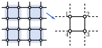
To be specific, we first partition the square lattice (including both layers) into square clusters as shown in Fig. 2. Let us first ignore the inter-cluster hopping. Within each cluster, we represent the Hamiltonian in the many-body Hilbert space and use the Lanczos method to obtain the lowest eigenvalues and eigenvectors. The Green’s function in the cluster can then be obtained by the Källén–Lehmann representation
| (15) |
where is the th excited state with energy , and is the ground state with energy , whose wave function was previously given in Eq. (5). Since the four fermion flavors (two spins and two layers) are identical under the internal flavor symmetry, we can drop the flavor index in the Green’s function and only focus on one particular flavor with the site indices , where as indicated in Fig. 2. The convergence of the Green’s function can be verified by including more eigenstates from the Lanczos method. We checked that increasing the number of eigenpairs to will not change the result significantly, indicating that the result with eigenpairs has already converged.
Now we restore the inter-cluster hoping to extend the Green’s function from small clusters to the infinite lattice. The Green’s function of super-lattice momentum can be obtained from the random phase approximation (RPA) approach [94],
| (16) |
where the matrix
| (17) |
describes the inter-cluster fermion hopping. The resulting Green’s function is defined in the folded Brillouin zone with sub-lattice indices . To unfold the Green’s function to the original Brillouin zone , we perform the following (partial) Fourier transform
| (18) |
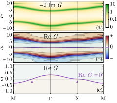
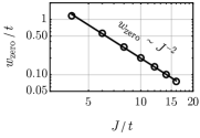
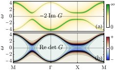
We numerically calculated the unfolded Green’s function using the above-mentioned cluster perturbation method. We take a large interaction strength deep in the SMG phase and present the resulting Green’s function in Fig. 3. From Fig. 3(a), the poles of the Green’s function form two dispersing bands around , which resembles the upper and lower Hubbard bands in the Hubbard model. This indicates the quasi-particles are fully gapped in the SMG phase. Meanwhile, from Fig. 3(b,c), the zeros of the Green’s function appear around with some non-universal but positive coefficient . We find that the “dispersion” of zeros is reversed compared to the original band dispersion . In Fig. 4, we also numerically confirmed that the “bandwidth” of zeros is suppressed by the interaction as as .
Building upon the above observation of the poles and zeros of the Green’s function, we put forth the following empirical formula:
| (19) |
as an approximate description of our numerical result Eq. (18). An important aspect of this formula is the positioning of the Green’s function zeros precisely around the initial Fermi surface (where ) at . This is indicated by the small arrows in Fig. 3(c).
Assuming as the definition of the zero Fermi surface in the SMG phase, it would encompass the same Fermi volume as the pole Fermi surface in the Fermi liquid phase. As both translation and charge conservation symmetries remain unbroken in the SMG phase, the Luttinger theorem mandates the preservation of the Fermi volume. Given that the SMG state is a fully gapped trivial insulator, there is no pole (no quasi-particle) at low energy, thus the Green’s function can only rely on zeros to fulfill the Fermi volume required by the Luttinger theorem, which is explicitly demonstrated by Eq. (19).
III.2 Weak Coupling Analysis
Nevertheless, SMG is not the sole mechanism for gapping out the Fermi surface. SSB might also open a full gap on the Fermi surface, which corresponds to the Higgs mechanism for fermion mass generation. Specifically, in the bilayer square lattice model Eq. (3), due to the perfect nesting of the Fermi surface, the Fermi liquid exhibits strong instability toward SSB orders. Without loss of generality, we will focus on the inter-layer exciton condensation in the weak coupling limit. The corresponding order parameter was introduced in Eq. (6), which carries momentum . The exciton condensation leads to an SSB insulating phase, as noted in the phase diagram Fig. 1(c). However, there are significant differences between the SMG insulator and the SSB insulator, especially in terms of the structure of Green’s function zeros.
In the SSB insulator phase, the Brillouin zone folds by the nesting vector . The fermion Green’s function can be written in the basis (omitting layers and spins freedom) as
| (20) |
where denotes the exciton gap induced by the exciton condensation . The properties of are illustrated in Fig. 5. The spectral function in Fig. 5(a) depicts the quasi-particle peak along the band dispersion, reflecting a gapped (insulating) band structure.
Since is a matrix, its zero structure should be defined by its determinant being zero, i.e., , which is the only way to define the zero structure in a basis independent manner. Fig. 5(b) indicates the determinant of remains the same sign within the band gap induced by the exciton condensation. Since does not preserve the translation symmetry (as is translation-odd), and is non-zero, does not have zeros crossing at the original Fermi surface. These two observations are linked: the absence of translation symmetry makes the Luttinger theorem ineffective, hence there is no expectation for the zero Fermi surface in the SSB insulator.
As the interaction intensifies, the SSB insulator ultimately transitions into the SMG insulator, as depicted in the phase diagram Fig. 1(c). During this transition, the broken symmetry is restored, yet the fermion excitation gap remains intact, similar to the pseudo-gap phenomenon seen in correlated materials [119, 120]. In the context of modeling fermion spectral functions, the pseudo-gap phenomenon can be interpreted as a consequence of the phase (or orientation) fluctuations of fermion bilinear order parameters [121, 122, 123, 124, 125, 126, 127, 128]. In this picture, the order parameter maintains a finite amplitude as we enter the SMG phase from the adjacent SSB phase, but its phase is disordered by long-wavelength random fluctuations. Consequently, on the large scale, cannot condense to form long-range order; but on a smaller scale, still provides a local excitation gap everywhere for fermions.
Based on this picture of the SMG state, the simplest treatment is to focus on the long wavelength fluctuation of and estimate its self-energy correction for the fermion by
| (21) |
where the vertex operator is and the bare Green’s function is . Here we have assumed that the correlation length of the bosonic field is long enough that its momentum is negligible for fermions. This assumption is valid near the transition to the SSB phase, as the correlation length diverges () at the transition.
Using this self-energy to correct the bare Green’s function, we obtain
| (22) |
Since the translation symmetry has been restored in the SMG phase, we can unfold the Green’s function back to the original Brillouin zone (by taking the component), which leads to a weak coupling description of the Green’s function in the shallow SMG phase near the transition to the SSB phase
| (23) |
A more rigorous treatment of a similar problem can be found in Ref. 95, which includes finite momentum fluctuations of . The major effect of these fluctuations is to introduce a spectral broadening for the fermion Green’s function as if replacing in Eq. (23). It was also found that the broadening scales inversely with the correlation length of the order parameter, which justifies our simple treatment in the large- regime. Similar Green’s functions as Eq. (23) was previously constructed to describe non-Fermi liquid [98] statisfying the Luttinger theorem. However, its physical meaning is now clarified as Green’s function in the SMG phase.
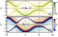
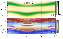
The features of in Eq. (23) are presented in Fig. 6. When comparing Fig. 6(a) and Fig. 5(a), we can observe that the pole structure of is identical to that of (in the diagonal component), both showcasing a gapped spectrum. However, they significantly differ in their zero structures, as seen by comparing Fig. 6(b) and Fig. 5(b). Due to the restoration of symmetry, the low-energy zeros reemerge in the Green’s function in the SMG phase. Additionally, its zero Fermi surface perfectly aligns with the original pole Fermi surface, fulfilling the Luttinger theorem’s requirement for the Fermi volume.
Comparing the Green’s function in the SMG phase derived from the strong coupling analysis Eq. (19) and the weak coupling analysis Eq. (23) (see also Fig. 3 and Fig. 6), we find that despite the apparent difference in high-energy spectral features, the zero Fermi surface defined by remains a resilient low-energy feature. The persistent zero Fermi surface in the SMG phase is a consequence of the Luttinger theorem.
Nonetheless, besides the low-energy zero structure, it is also intriguing to understand how the high-energy spectral feature deforms from the weak coupling case to the strong coupling case. However, this problem requires non-perturbative numerical simulations. Fortunately, the bilayer square lattice model Eq. (3) admits a sign-problem-free [129] quantum Monte Carlo [130, 131, 132, 133, 134] simulation. We will leave this interesting direction for future research.
IV Probing Green’s Function Zeros
While Green’s function zeros are an important feature of the SMG insulator, they are not directly observable in experiments. Spectroscopy experiments, such as angle-resolved photoemission spectroscopy (ARPES), can directly probe the fermion’s spectral function , which is the imaginary part of Green’s function. By employing the Kramers-Kronig (KK) relation to recover the real part of Green’s function from the spectral function,
| (24) |
we can indirectly study the zero structure of the Green’s function.
However, the spectral function might be broadened in experimental data due to noise or dissipation. We are interested in studying how sensitive the reconstructed Green’s function zero is to these disturbances, in order to understand the stability of the method. Following Sec. III.1, we start from the strong coupling limit and use the CPT approach to calculate Green’s function. To account for the spectral broadening effect, we replace with , where is relatively large, say, about the order of the hopping . Based on the broadened spectral function in Fig. 7(a), we use the KK relation to reconstruct the real part, as shown in Fig. 7(b). We find that the zero Fermi surface maintains the same shape, but the zero “dispersion” bandwidth gets larger.
The increase in bandwidth can be understood by taking the SMG Green’s function in Eq. (19), and solving for its zeros . To the leading order of and , the solution is given by
| (25) |
meaning that the bandwidth of Green’s function zero dispersion will increase by , but the corresponding Luttinger surface remains unchanged. Therefore, the Green’s function zero in the SMG phase is a robust feature that can be potentially identified from spectroscopy measurements, even in the presence of noises or dissipations.
V Summary and Discussions
In this paper, we investigated the Fermi surface SMG in a bilayer square lattice model. A crucial finding of this study lies in the robust Green’s function zero in the SMG phase. Traditionally, a Fermi liquid state is characterized by poles in the Green’s function along the Fermi surface. However, as the fermion system is driven into the SMG state by interaction effects, these poles are replaced by zeros. This is a robust phenomenon underlined by the constraints of the Luttinger theorem.
Our exploration is not limited to theoretical assertions. We also offer a tangible demonstration of this occurrence in the bilayer square lattice model. By applying both strong and weak coupling analyses, we provide a comprehensive portrayal of the fermion Green’s function across different interaction regimes. We highlight that the emergence of the zero Fermi surface is not an ephemeral or fine-tuned phenomenon, but rather a robust and enduring feature of the SMG phase. We show that even when the system is subjected to spectral broadening, the zero Fermi surface persists, retaining the Fermi volume.
The results of this study confirm the robustness of the zero Fermi surface and underscore the possibility of observing it in experimental setups, such as through ARPES. Despite not being directly observable, the zero structure of the Green’s function could be inferred indirectly via the KK relation.
The bilayer square lattice model may be relevant to the nickelate superconductor recently discovered in pressurized La3Ni2O7 [135, 136], which is a layered two-dimensional material where each layer consists of nickel atoms arranged in a bilayer square lattice. The Fermi surface is dominated by and electrons of Ni. The electron has a relatively small intra-layer hopping due to the rather localized orbital wave function in the -plane but enjoys a large interlayer antiferromagnetic Heisenberg interaction due to the super-exchange mechanism mediated by the apical oxygen. This likely puts the electrons in an SMG insulator phase in the bilayer square lattice model and opens up opportunities to investigate the proposed Green’s function zeros in real materials. The potential implication of SMG physics on the nickelate high- superconductor still requires further theoretical research in the future.
Acknowledgements.
We acknowledge the helpful discussions with Liujun Zou, Zi-Xiang Li, Fan Yang, Yang Qi, Subir Sachdev, and Ya-Hui Zhang. All authors are supported by the NSF Grant DMR-2238360.References
- Fidkowski and Kitaev [2010] L. Fidkowski and A. Kitaev, Effects of interactions on the topological classification of free fermion systems, Phys. Rev. B 81, 134509 (2010), arXiv:0904.2197 [cond-mat.str-el] .
- Fidkowski and Kitaev [2011] L. Fidkowski and A. Kitaev, Topological phases of fermions in one dimension, Phys. Rev. B 83, 075103 (2011), arXiv:1008.4138 [cond-mat.str-el] .
- Wang and Wen [2023] J. Wang and X.-G. Wen, Non-Perturbative Regularization of 1+1D Anomaly-Free Chiral Fermions and Bosons: On the equivalence of anomaly matching conditions and boundary gapping rules, Phys. Rev. B 107, 014311 (2023), arXiv:1307.7480 [hep-lat] .
- Slagle et al. [2015] K. Slagle, Y.-Z. You, and C. Xu, Exotic quantum phase transitions of strongly interacting topological insulators, Phys. Rev. B 91, 115121 (2015), arXiv:1409.7401 [cond-mat.str-el] .
- Ayyar and Chandrasekharan [2015] V. Ayyar and S. Chandrasekharan, Massive fermions without fermion bilinear condensates, Phys. Rev. D 91, 065035 (2015), arXiv:1410.6474 [hep-lat] .
- Catterall [2016] S. Catterall, Fermion mass without symmetry breaking, Journal of High Energy Physics 1, 121 (2016), arXiv:1510.04153 [hep-lat] .
- Tong [2022] D. Tong, Comments on symmetric mass generation in 2d and 4d, Journal of High Energy Physics 2022, 1 (2022), arXiv:2104.03997 [hep-th] .
- Wang and You [2022] J. Wang and Y.-Z. You, Symmetric Mass Generation, Symmetry 14, 1475 (2022), arXiv:2204.14271 [cond-mat.str-el] .
- Nambu [1960] Y. Nambu, Quasi-Particles and Gauge Invariance in the Theory of Superconductivity, Physical Review 117, 648 (1960).
- Nambu and Jona-Lasinio [1961] Y. Nambu and G. Jona-Lasinio, Dynamical Model of Elementary Particles Based on an Analogy with Superconductivity. I, Physical Review 122, 345 (1961).
- Goldstone et al. [1962] J. Goldstone, A. Salam, and S. Weinberg, Broken Symmetries, Physical Review 127, 965 (1962).
- Anderson [1963] P. W. Anderson, Plasmons, Gauge Invariance, and Mass, Physical Review 130, 439 (1963).
- Englert and Brout [1964] F. Englert and R. Brout, Broken Symmetry and the Mass of Gauge Vector Mesons, Phys. Rev. Lett. 13, 321 (1964).
- Higgs [1964] P. W. Higgs, Broken Symmetries and the Masses of Gauge Bosons, Phys. Rev. Lett. 13, 508 (1964).
- Nielsen and Ninomiya [1981] H. B. Nielsen and M. Ninomiya, Absence of neutrinos on a lattice: (ii). intuitive topological proof, Nuclear Physics B 193, 173 (1981).
- Nielsen and Ninomiya [1981a] H. B. Nielsen and M. Ninomiya, Absence of neutrinos on a lattice (I). Proof by homotopy theory, Nuclear Physics B 185, 20 (1981a).
- Nielsen and Ninomiya [1981b] H. B. Nielsen and M. Ninomiya, A no-go theorem for regularizing chiral fermions, Physics Letters B 105, 219 (1981b).
- Swift [1984] P. Swift, The electroweak theory on the lattice, Physics Letters B 145, 256 (1984).
- Eichten and Preskill [1986] E. Eichten and J. Preskill, Chiral Gauge Theories on the Lattice, Nucl. Phys. B 268, 179 (1986).
- Smit [1986] J. Smit, Fermions on a Lattice, Acta Phys. Polon. B 17, 531 (1986).
- Kaplan [1992] D. B. Kaplan, A method for simulating chiral fermions on the lattice, Physics Letters B 288, 342 (1992).
- Wen [2013] X.-G. Wen, A Lattice Non-Perturbative Definition of an SO(10) Chiral Gauge Theory and Its Induced Standard Model, Chinese Physics Letters 30, 111101 (2013), arXiv:1305.1045 [hep-lat] .
- You et al. [2014a] Y.-Z. You, Y. BenTov, and C. Xu, Interacting Topological Superconductors and possible Origin of Chiral Fermions in the Standard Model, ArXiv e-prints (2014a), arXiv:1402.4151 [cond-mat.str-el] .
- You and Xu [2015] Y.-Z. You and C. Xu, Interacting topological insulator and emergent grand unified theory, Phys. Rev. B 91, 125147 (2015), arXiv:1412.4784 [cond-mat.str-el] .
- BenTov [2015] Y. BenTov, Fermion masses without symmetry breaking in two spacetime dimensions, Journal of High Energy Physics 7, 34 (2015), arXiv:1412.0154 [cond-mat.str-el] .
- Ayyar and Chandrasekharan [2016a] V. Ayyar and S. Chandrasekharan, Origin of fermion masses without spontaneous symmetry breaking, Phys. Rev. D 93, 081701 (2016a), arXiv:1511.09071 [hep-lat] .
- Ayyar and Chandrasekharan [2016b] V. Ayyar and S. Chandrasekharan, Fermion masses through four-fermion condensates, Journal of High Energy Physics 10, 58 (2016b), arXiv:1606.06312 [hep-lat] .
- Ayyar [2016] V. Ayyar, Search for a continuum limit of the PMS phase, ArXiv e-prints (2016), arXiv:1611.00280 [hep-lat] .
- DeMarco and Wen [2017] M. DeMarco and X.-G. Wen, A Novel Non-Perturbative Lattice Regularization of an Anomaly-Free Chiral Gauge Theory, arXiv e-prints , arXiv:1706.04648 (2017), arXiv:1706.04648 [hep-lat] .
- Ayyar and Chandrasekharan [2017] V. Ayyar and S. Chandrasekharan, Generating a nonperturbative mass gap using Feynman diagrams in an asymptotically free theory, Phys. Rev. D 96, 114506 (2017), arXiv:1709.06048 [hep-lat] .
- Schaich and Catterall [2018] D. Schaich and S. Catterall, Phases of a strongly coupled four-fermion theory, in European Physical Journal Web of Conferences, European Physical Journal Web of Conferences, Vol. 175 (2018) p. 03004, arXiv:1710.08137 [hep-lat] .
- Butt and Catterall [2018] N. Butt and S. Catterall, Four fermion condensates in SU(2) Yang-Mills-Higgs theory on a lattice, in The 36th Annual International Symposium on Lattice Field Theory. 22-28 July (2018) p. 294, arXiv:1811.01015 [hep-lat] .
- Butt et al. [2018] N. Butt, S. Catterall, and D. Schaich, SO(4) invariant Higgs-Yukawa model with reduced staggered fermions, Phys. Rev. D 98, 114514 (2018), arXiv:1810.06117 [hep-lat] .
- Kikukawa [2019a] Y. Kikukawa, On the gauge-invariant path-integral measure for the overlap Weyl fermions in 16 of SO(10), Progress of Theoretical and Experimental Physics 2019, 113B03 (2019a).
- Kikukawa [2019b] Y. Kikukawa, Why is the mission impossible? Decoupling the mirror Ginsparg-Wilson fermions in the lattice models for two-dimensional Abelian chiral gauge theories, Progress of Theoretical and Experimental Physics 2019, 073B02 (2019b), arXiv:1710.11101 [hep-lat] .
- Wang and Wen [2019] J. Wang and X.-G. Wen, Solution to the 1 +1 dimensional gauged chiral Fermion problem, Phys. Rev. D 99, 111501 (2019), arXiv:1807.05998 [hep-lat] .
- Wang and Wen [2020] J. Wang and X.-G. Wen, Nonperturbative definition of the standard models, Physical Review Research 2, 023356 (2020), arXiv:1809.11171 [hep-th] .
- Catterall et al. [2020] S. Catterall, N. Butt, and D. Schaich, Exotic Phases of a Higgs-Yukawa Model with Reduced Staggered Fermions, arXiv e-prints , arXiv:2002.00034 (2020), arXiv:2002.00034 [hep-lat] .
- Razamat and Tong [2021] S. S. Razamat and D. Tong, Gapped Chiral Fermions, Physical Review X 11, 011063 (2021), arXiv:2009.05037 [hep-th] .
- Catterall [2021] S. Catterall, Chiral lattice fermions from staggered fields, Phys. Rev. D 104, 014503 (2021), arXiv:2010.02290 [hep-lat] .
- Butt et al. [2021a] N. Butt, S. Catterall, A. Pradhan, and G. C. Toga, Anomalies and symmetric mass generation for Kähler-Dirac fermions, Phys. Rev. D 104, 094504 (2021a), arXiv:2101.01026 [hep-th] .
- Butt et al. [2021b] N. Butt, S. Catterall, and G. C. Toga, Symmetric Mass Generation in Lattice Gauge Theory, arXiv e-prints , arXiv:2111.01001 (2021b), arXiv:2111.01001 [hep-lat] .
- Zeng et al. [2022] M. Zeng, Z. Zhu, J. Wang, and Y.-Z. You, Symmetric Mass Generation in the 1 +1 Dimensional Chiral Fermion 3-4-5-0 Model, Phys. Rev. Lett. 128, 185301 (2022), arXiv:2202.12355 [cond-mat.str-el] .
- Catterall and Pradhan [2022] S. Catterall and A. Pradhan, Induced topological gravity and anomaly inflow from Kähler-Dirac fermions in odd dimensions, Phys. Rev. D 106, 014509 (2022), arXiv:2201.00750 [hep-th] .
- Catterall [2023] S. Catterall, ’t Hooft anomalies for staggered fermions, Phys. Rev. D 107, 014501 (2023), arXiv:2209.03828 [hep-lat] .
- Guo and You [2023] Y. Guo and Y.-Z. You, Symmetric Mass Generation of Kähler-Dirac Fermions from the Perspective of Symmetry-Protected Topological Phases, arXiv e-prints , arXiv:2306.17420 (2023), arXiv:2306.17420 [cond-mat.str-el] .
- Turner et al. [2011] A. M. Turner, F. Pollmann, and E. Berg, Topological phases of one-dimensional fermions: An entanglement point of view, Phys. Rev. B 83, 075102 (2011), arXiv:1008.4346 [cond-mat.str-el] .
- Ryu and Zhang [2012] S. Ryu and S.-C. Zhang, Interacting topological phases and modular invariance, Phys. Rev. B 85, 245132 (2012), arXiv:1202.4484 [cond-mat.str-el] .
- Qi [2013] X.-L. Qi, A new class of (2 + 1)-dimensional topological superconductors with topological classification, New Journal of Physics 15, 065002 (2013), arXiv:1202.3983 [cond-mat.str-el] .
- Yao and Ryu [2013] H. Yao and S. Ryu, Interaction effect on topological classification of superconductors in two dimensions, Phys. Rev. B 88, 064507 (2013), arXiv:1202.5805 [cond-mat.str-el] .
- Gu and Levin [2014] Z.-C. Gu and M. Levin, Effect of interactions on two-dimensional fermionic symmetry-protected topological phases with Z2 symmetry, Phys. Rev. B 89, 201113 (2014), arXiv:1304.4569 [cond-mat.str-el] .
- Wang and Senthil [2014] C. Wang and T. Senthil, Interacting fermionic topological insulators/superconductors in three dimensions, Phys. Rev. B 89, 195124 (2014), arXiv:1401.1142 [cond-mat.str-el] .
- Metlitski et al. [2014] M. A. Metlitski, L. Fidkowski, X. Chen, and A. Vishwanath, Interaction effects on 3D topological superconductors: surface topological order from vortex condensation, the 16 fold way and fermionic Kramers doublets, arXiv e-prints , arXiv:1406.3032 (2014), arXiv:1406.3032 [cond-mat.str-el] .
- Kapustin et al. [2015] A. Kapustin, R. Thorngren, A. Turzillo, and Z. Wang, Fermionic symmetry protected topological phases and cobordisms, Journal of High Energy Physics 2015, 52 (2015), arXiv:1406.7329 [cond-mat.str-el] .
- You and Xu [2014] Y.-Z. You and C. Xu, Symmetry-protected topological states of interacting fermions and bosons, Phys. Rev. B 90, 245120 (2014), arXiv:1409.0168 [cond-mat.str-el] .
- Cheng et al. [2015] M. Cheng, Z. Bi, Y.-Z. You, and Z.-C. Gu, Classification of Symmetry-Protected Phases for Interacting Fermions in Two Dimensions, arXiv e-prints , arXiv:1501.01313 (2015), arXiv:1501.01313 [cond-mat.str-el] .
- Yoshida and Furusaki [2015] T. Yoshida and A. Furusaki, Correlation effects on topological crystalline insulators, Phys. Rev. B 92, 085114 (2015), arXiv:1505.06598 [cond-mat.str-el] .
- Gu and Qi [2015] Y. Gu and X.-L. Qi, Axion field theory approach and the classification of interacting topological superconductors, ArXiv e-prints (2015), arXiv:1512.04919 [cond-mat.supr-con] .
- Song and Schnyder [2016] X.-Y. Song and A. P. Schnyder, Interaction effects on the classification of crystalline topological insulators and superconductors, ArXiv e-prints (2016), arXiv:1609.07469 [cond-mat.str-el] .
- Queiroz et al. [2016] R. Queiroz, E. Khalaf, and A. Stern, Dimensional Hierarchy of Fermionic Interacting Topological Phases, Physical Review Letters 117, 206405 (2016), arXiv:1601.01596 [cond-mat.str-el] .
- Witten [2016] E. Witten, The “parity” anomaly on an unorientable manifold, Phys. Rev. B 94, 195150 (2016), arXiv:1605.02391 [hep-th] .
- Wang and Gu [2017] Q.-R. Wang and Z.-C. Gu, Towards a complete classification of fermionic symmetry protected topological phases in 3D and a general group supercohomology theory, ArXiv e-prints (2017), arXiv:1703.10937 [cond-mat.str-el] .
- Kapustin and Thorngren [2017] A. Kapustin and R. Thorngren, Fermionic SPT phases in higher dimensions and bosonization, Journal of High Energy Physics 2017, 80 (2017), arXiv:1701.08264 [cond-mat.str-el] .
- Wang et al. [2018] J. Wang, K. Ohmori, P. Putrov, Y. Zheng, Z. Wan, M. Guo, H. Lin, P. Gao, and S.-T. Yau, Tunneling topological vacua via extended operators: (Spin-)TQFT spectra and boundary deconfinement in various dimensions, Progress of Theoretical and Experimental Physics 2018, 053A01 (2018), arXiv:1801.05416 [cond-mat.str-el] .
- Wang and Gu [2018] Q.-R. Wang and Z.-C. Gu, Construction and classification of symmetry protected topological phases in interacting fermion systems, arXiv e-prints , arXiv:1811.00536 (2018), arXiv:1811.00536 [cond-mat.str-el] .
- Guo et al. [2020] M. Guo, K. Ohmori, P. Putrov, Z. Wan, and J. Wang, Fermionic Finite-Group Gauge Theories and Interacting Symmetric/Crystalline Orders via Cobordisms, Communications in Mathematical Physics 376, 1073 (2020), arXiv:1812.11959 [hep-th] .
- Aasen et al. [2021] D. Aasen, P. Bonderson, and C. Knapp, Characterization and Classification of Fermionic Symmetry Enriched Topological Phases, arXiv e-prints , arXiv:2109.10911 (2021), arXiv:2109.10911 [cond-mat.str-el] .
- Barkeshli et al. [2022] M. Barkeshli, Y.-A. Chen, P.-S. Hsin, and N. Manjunath, Classification of (2 +1 )D invertible fermionic topological phases with symmetry, Phys. Rev. B 105, 235143 (2022), arXiv:2109.11039 [cond-mat.str-el] .
- Zou and Chowdhury [2020a] L. Zou and D. Chowdhury, Deconfined Metal-Insulator Transitions in Quantum Hall Bilayers, arXiv e-prints , arXiv:2004.14391 (2020a), arXiv:2004.14391 [cond-mat.str-el] .
- Zhang and Sachdev [2020a] Y.-H. Zhang and S. Sachdev, From the pseudogap metal to the Fermi liquid using ancilla qubits, Physical Review Research 2, 023172 (2020a), arXiv:2001.09159 [cond-mat.str-el] .
- Zou and Chowdhury [2020b] L. Zou and D. Chowdhury, Deconfined metallic quantum criticality: A U(2) gauge-theoretic approach, Physical Review Research 2, 023344 (2020b), arXiv:2002.02972 [cond-mat.str-el] .
- Zhang and Sachdev [2020b] Y.-H. Zhang and S. Sachdev, Deconfined criticality and ghost Fermi surfaces at the onset of antiferromagnetism in a metal, Phys. Rev. B 102, 155124 (2020b), arXiv:2006.01140 [cond-mat.str-el] .
- Nikolaenko et al. [2021] A. Nikolaenko, M. Tikhanovskaya, S. Sachdev, and Y.-H. Zhang, Small to large Fermi surface transition in a single-band model using randomly coupled ancillas, Phys. Rev. B 103, 235138 (2021), arXiv:2103.05009 [cond-mat.str-el] .
- Lu et al. [2022] D.-C. Lu, M. Zeng, J. Wang, and Y.-Z. You, Fermi Surface Symmetric Mass Generation, arXiv e-prints , arXiv:2210.16304 (2022), arXiv:2210.16304 [cond-mat.str-el] .
- Bulmash et al. [2015] D. Bulmash, P. Hosur, S.-C. Zhang, and X.-L. Qi, Unified Topological Response Theory For Gapped and Gapless Free Fermions, Physical Review X 5, 021018 (2015), arXiv:1410.4202 [cond-mat.mes-hall] .
- Lu et al. [2023] D.-C. Lu, J. Wang, and Y.-Z. You, Definition and Classification of Fermi Surface Anomalies, arXiv e-prints , arXiv:2302.12731 (2023), arXiv:2302.12731 [cond-mat.str-el] .
- Gurarie [2011] V. Gurarie, Single-particle Green’s functions and interacting topological insulators, Phys. Rev. B 83, 085426 (2011), arXiv:1011.2273 [cond-mat.mes-hall] .
- You et al. [2014b] Y.-Z. You, Z. Wang, J. Oon, and C. Xu, Topological number and fermion Green’s function for strongly interacting topological superconductors, Phys. Rev. B 90, 060502 (2014b), arXiv:1403.4938 [cond-mat.str-el] .
- Catterall and Schaich [2016] S. Catterall and D. Schaich, Novel phases in strongly coupled four-fermion theories, ArXiv e-prints (2016), arXiv:1609.08541 [hep-lat] .
- You et al. [2018a] Y.-Z. You, Y.-C. He, C. Xu, and A. Vishwanath, Symmetric Fermion Mass Generation as Deconfined Quantum Criticality, Physical Review X 8, 011026 (2018a), arXiv:1705.09313 [cond-mat.str-el] .
- Catterall and Butt [2018] S. Catterall and N. Butt, Topology and strong four fermion interactions in four dimensions, Phys. Rev. D 97, 094502 (2018), arXiv:1708.06715 [hep-lat] .
- Xu and Xu [2021] Y. Xu and C. Xu, Green’s function Zero and Symmetric Mass Generation, arXiv e-prints , arXiv:2103.15865 (2021), arXiv:2103.15865 [cond-mat.str-el] .
- You et al. [2018b] Y.-Z. You, Y.-C. He, A. Vishwanath, and C. Xu, From bosonic topological transition to symmetric fermion mass generation, Phys. Rev. B 97, 125112 (2018b), arXiv:1711.00863 [cond-mat.str-el] .
- Wang et al. [2021] C. Wang, A. Hickey, X. Ying, and A. A. Burkov, Emergent anomalies and generalized Luttinger theorems in metals and semimetals, Phys. Rev. B 104, 235113 (2021), arXiv:2110.10692 [cond-mat.str-el] .
- Wen [2021] X.-G. Wen, Low-energy effective field theories of fermion liquids and the mixed U (1 ) ×Rd anomaly, Phys. Rev. B 103, 165126 (2021), arXiv:2101.08772 [cond-mat.str-el] .
- Cheng et al. [2016] M. Cheng, M. Zaletel, M. Barkeshli, A. Vishwanath, and P. Bonderson, Translational Symmetry and Microscopic Constraints on Symmetry-Enriched Topological Phases: A View from the Surface, Physical Review X 6, 041068 (2016), arXiv:1511.02263 [cond-mat.str-el] .
- Cho et al. [2017] G. Y. Cho, C.-T. Hsieh, and S. Ryu, Anomaly manifestation of Lieb-Schultz-Mattis theorem and topological phases, Phys. Rev. B 96, 195105 (2017), arXiv:1705.03892 [cond-mat.str-el] .
- Bultinck and Cheng [2018] N. Bultinck and M. Cheng, Filling constraints on fermionic topological order in zero magnetic field, Phys. Rev. B 98, 161119 (2018), arXiv:1808.00324 [cond-mat.str-el] .
- Thorngren and Else [2018] R. Thorngren and D. V. Else, Gauging Spatial Symmetries and the Classification of Topological Crystalline Phases, Physical Review X 8, 011040 (2018).
- Cheng and Seiberg [2022] M. Cheng and N. Seiberg, Lieb-Schultz-Mattis, Luttinger, and ’t Hooft – anomaly matching in lattice systems, arXiv e-prints , arXiv:2211.12543 (2022), arXiv:2211.12543 [cond-mat.str-el] .
- Else et al. [2021] D. V. Else, R. Thorngren, and T. Senthil, Non-Fermi Liquids as Ersatz Fermi Liquids: General Constraints on Compressible Metals, Physical Review X 11, 021005 (2021), arXiv:2007.07896 [cond-mat.str-el] .
- Else and Senthil [2021] D. V. Else and T. Senthil, Strange Metals as Ersatz Fermi Liquids, Phys. Rev. Lett. 127, 086601 (2021), arXiv:2010.10523 [cond-mat.str-el] .
- Darius Shi et al. [2022] Z. Darius Shi, H. Goldman, D. V. Else, and T. Senthil, Gifts from anomalies: Exact results for Landau phase transitions in metals, SciPost Phys. 13, 102 (2022), arXiv:2204.07585 [cond-mat.str-el] .
- Sénéchal et al. [2000] D. Sénéchal, D. Perez, and M. Pioro-Ladrière, Spectral Weight of the Hubbard Model through Cluster Perturbation Theory, Phys. Rev. Lett. 84, 522 (2000), arXiv:cond-mat/9908045 [cond-mat.str-el] .
- Wang and Qi [2023] X.-C. Wang and Y. Qi, Phase fluctuations in two-dimensional superconductors and pseudogap phenomenon, Phys. Rev. B 107, 224502 (2023), arXiv:2212.05737 [cond-mat.supr-con] .
- Altshuler et al. [1998] B. L. Altshuler, A. V. Chubukov, A. Dashevskii, A. M. Finkel’stein, and D. K. Morr, Luttinger theorem for a spin-density-wave state, EPL (Europhysics Letters) 41, 401 (1998), arXiv:cond-mat/9703120 [cond-mat.str-el] .
- Oshikawa [2000] M. Oshikawa, Topological Approach to Luttinger’s Theorem and the Fermi Surface of a Kondo Lattice, Phys. Rev. Lett. 84, 3370 (2000), arXiv:cond-mat/0002392 [cond-mat.str-el] .
- Dzyaloshinskii [2003] I. Dzyaloshinskii, Some consequences of the Luttinger theorem: The Luttinger surfaces in non-Fermi liquids and Mott insulators, Phys. Rev. B 68, 085113 (2003).
- Gnezdilov and Wang [2022] N. V. Gnezdilov and Y. Wang, Solvable model for a charge-4 e superconductor, Phys. Rev. B 106, 094508 (2022), arXiv:2111.09906 [cond-mat.str-el] .
- Luttinger [1960] J. M. Luttinger, Fermi surface and some simple equilibrium properties of a system of interacting fermions, Phys. Rev. 119, 1153 (1960).
- Stanescu et al. [2007] T. D. Stanescu, P. Phillips, and T.-P. Choy, Theory of the Luttinger surface in doped Mott insulators, Phys. Rev. B 75, 104503 (2007), arXiv:cond-mat/0602280 [cond-mat.str-el] .
- Scheurer et al. [2018] M. S. Scheurer, S. Chatterjee, W. Wu, M. Ferrero, A. Georges, and S. Sachdev, Topological order in the pseudogap metal, Proceedings of the National Academy of Science 115, E3665 (2018), arXiv:1711.09925 [cond-mat.str-el] .
- Xiang and Wu [2022] T. Xiang and C. Wu, D-wave Superconductivity (Cambridge University Press, 2022) Chap. 4.
- Zhai et al. [2009] H. Zhai, F. Wang, and D.-H. Lee, Antiferromagnetically driven electronic correlations in iron pnictides and cuprates, Phys. Rev. B 80, 064517 (2009), arXiv:0905.1711 [cond-mat.supr-con] .
- Rüger et al. [2014] R. Rüger, L. F. Tocchio, R. Valentí, and C. Gros, The phase diagram of the square lattice bilayer Hubbard model: a variational Monte Carlo study, New Journal of Physics 16, 033010 (2014), arXiv:1311.6504 [cond-mat.str-el] .
- Rhim and Yang [2019] J.-W. Rhim and B.-J. Yang, Classification of flat bands according to the band-crossing singularity of Bloch wave functions, Phys. Rev. B 99, 045107 (2019), arXiv:1808.05926 [cond-mat.str-el] .
- Chao et al. [1978] K. A. Chao, J. Spałek, and A. M. Oleś, Canonical perturbation expansion of the hubbard model, Phys. Rev. B 18, 3453 (1978).
- Gutzwiller [1964] M. C. Gutzwiller, Effect of correlation on the ferromagnetism of transition metals, Phys. Rev. 134, A923 (1964).
- Hou and You [2022] W. Hou and Y.-Z. You, Variational Monte Carlo Study of Symmetric Mass Generation in a Bilayer Honeycomb Lattice Model, arXiv e-prints , arXiv:2212.13364 (2022), arXiv:2212.13364 [cond-mat.str-el] .
- Luttinger and Ward [1960] J. M. Luttinger and J. C. Ward, Ground-state energy of a many-fermion system. ii, Phys. Rev. 118, 1417 (1960).
- Senthil et al. [2003] T. Senthil, S. Sachdev, and M. Vojta, Fractionalized Fermi Liquids, Phys. Rev. Lett. 90, 216403 (2003), arXiv:cond-mat/0209144 [cond-mat.str-el] .
- Senthil et al. [2004] T. Senthil, M. Vojta, and S. Sachdev, Weak magnetism and non-Fermi liquids near heavy-fermion critical points, Phys. Rev. B 69, 035111 (2004), arXiv:cond-mat/0305193 [cond-mat.str-el] .
- Paramekanti and Vishwanath [2004] A. Paramekanti and A. Vishwanath, Extending Luttinger’s theorem to fractionalized phases of matter, Phys. Rev. B 70, 245118 (2004), arXiv:cond-mat/0406619 [cond-mat.str-el] .
- Oshikawa and Senthil [2006] M. Oshikawa and T. Senthil, Fractionalization, Topological Order, and Quasiparticle Statistics, Phys. Rev. Lett. 96, 060601 (2006), arXiv:cond-mat/0506008 [cond-mat.str-el] .
- Nandkishore et al. [2012] R. Nandkishore, M. A. Metlitski, and T. Senthil, Orthogonal metals: The simplest non-Fermi liquids, Phys. Rev. B 86, 045128 (2012), arXiv:1201.5998 [cond-mat.str-el] .
- Sachdev [2019] S. Sachdev, Topological order, emergent gauge fields, and Fermi surface reconstruction, Reports on Progress in Physics 82, 014001 (2019), arXiv:1801.01125 [cond-mat.str-el] .
- Skolimowski and Fabrizio [2022] J. Skolimowski and M. Fabrizio, Luttinger’s theorem in the presence of Luttinger surfaces, Phys. Rev. B 106, 045109 (2022), arXiv:2202.00426 [cond-mat.str-el] .
- Sénéchal et al. [2002] D. Sénéchal, D. Perez, and D. Plouffe, Cluster perturbation theory for Hubbard models, Phys. Rev. B 66, 075129 (2002), arXiv:cond-mat/0205044 [cond-mat.str-el] .
- Lee et al. [2006] P. A. Lee, N. Nagaosa, and X.-G. Wen, Doping a Mott Insulator: Physics of High Temperature Superconductivity, Rev. Mod. Phys. 78, 17 (2006), arXiv:cond-mat/0410445 [cond-mat.str-el] .
- Keimer et al. [2015] B. Keimer, S. A. Kivelson, M. R. Norman, S. Uchida, and J. Zaanen, From quantum matter to high-temperature superconductivity in copper oxides, Nature 518, 179 (2015), arXiv:1409.4673 [cond-mat.supr-con] .
- Franz and Millis [1998] M. Franz and A. J. Millis, Phase fluctuations and spectral properties of underdoped cuprates, Phys. Rev. B 58, 14572 (1998), arXiv:cond-mat/9805401 [cond-mat.supr-con] .
- Kwon and Dorsey [1999] H.-J. Kwon and A. T. Dorsey, Effect of phase fluctuations on the single-particle properties of underdoped cuprates, Phys. Rev. B 59, 6438 (1999), arXiv:cond-mat/9809225 [cond-mat.supr-con] .
- Kwon et al. [2001] H.-J. Kwon, A. T. Dorsey, and P. J. Hirschfeld, Observability of Quantum Phase Fluctuations in Cuprate Superconductors, Phys. Rev. Lett. 86, 3875 (2001), arXiv:cond-mat/0006290 [cond-mat.supr-con] .
- Franz and Tešanović [2001] M. Franz and Z. Tešanović, Algebraic Fermi Liquid from Phase Fluctuations: “Topological“ Fermions, Vortex “Berryons,” and QED3 Theory of Cuprate Superconductors, Phys. Rev. Lett. 87, 257003 (2001), arXiv:cond-mat/0012445 [cond-mat.supr-con] .
- Curty and Beck [2003] P. Curty and H. Beck, Thermodynamics and Phase Diagram of High Temperature Superconductors, Phys. Rev. Lett. 91, 257002 (2003), arXiv:cond-mat/0401124 [cond-mat.supr-con] .
- Li and Yao [2018a] T. Li and D.-W. Yao, Pairing origin of the pseudogap as observed in ARPES measurement in the underdoped cuprates, arXiv e-prints , arXiv:1805.05530 (2018a), arXiv:1805.05530 [cond-mat.supr-con] .
- Li and Yao [2018b] T. Li and D.-W. Yao, Why is the antinodal quasiparticle in the electron-doped cuprate Pr1.3-xLa0.7CexCuO4 immune to the antiferromagnetic band-folding effect?, EPL (Europhysics Letters) 124, 47001 (2018b), arXiv:1803.08226 [cond-mat.str-el] .
- Ye and Chubukov [2019] M. Ye and A. V. Chubukov, Hubbard model on a triangular lattice: Pseudogap due to spin density wave fluctuations, Phys. Rev. B 100, 035135 (2019), arXiv:1905.11412 [cond-mat.str-el] .
- Troyer and Wiese [2005] M. Troyer and U.-J. Wiese, Computational Complexity and Fundamental Limitations to Fermionic Quantum Monte Carlo Simulations, Phys. Rev. Lett. 94, 170201 (2005), arXiv:cond-mat/0408370 [cond-mat.stat-mech] .
- Fucito et al. [1981] F. Fucito, E. Marinari, G. Parisi, and C. Rebbi, A proposal for monte carlo simulations of fermionic systems, Nuclear Physics B 180, 369 (1981).
- Scalapino and Sugar [1981] D. J. Scalapino and R. L. Sugar, Method for performing monte carlo calculations for systems with fermions, Phys. Rev. Lett. 46, 519 (1981).
- Blankenbecler et al. [1981] R. Blankenbecler, D. J. Scalapino, and R. L. Sugar, Monte carlo calculations of coupled boson-fermion systems. i, Phys. Rev. D 24, 2278 (1981).
- Hirsch et al. [1981] J. E. Hirsch, D. J. Scalapino, R. L. Sugar, and R. Blankenbecler, Efficient monte carlo procedure for systems with fermions, Phys. Rev. Lett. 47, 1628 (1981).
- Hirsch [1985] J. E. Hirsch, Two-dimensional hubbard model: Numerical simulation study, Phys. Rev. B 31, 4403 (1985).
- Sun et al. [2023] H. Sun, M. Huo, X. Hu, J. Li, Z. Liu, Y. Han, L. Tang, Z. Mao, P. Yang, B. Wang, J. Cheng, D.-X. Yao, G.-M. Zhang, and M. Wang, Signatures of superconductivity near 80 k in a nickelate under high pressure, Nature 10.1038/s41586-023-06408-7 (2023).
- Hou et al. [2023] J. Hou, P. T. Yang, Z. Y. Liu, J. Y. Li, P. F. Shan, L. Ma, G. Wang, N. N. Wang, H. Z. Guo, J. P. Sun, Y. Uwatoko, M. Wang, G. M. Zhang, B. S. Wang, and J. G. Cheng, Emergence of high-temperature superconducting phase in the pressurized La3Ni2O7 crystals, arXiv e-prints , arXiv:2307.09865 (2023), arXiv:2307.09865 [cond-mat.supr-con] .
Appendix A Cluster Perturbation Theory
Here we review the details of cluster perturbation theory (CPT) originally developed in [94]. Denote the superlattice lattice points by , then the position of any original lattice point would be given by , where is the relative position of the lattice point to the location of the cluster containing that particular lattice point. For clusters of size , the generic Green’s function in real space can be denoted by , with , where the time-dependence is implicitly assumed and same goes for the frequency-dependence in Fourier space. Due to the translation invariance of the clusters on the superlattice, the real space Green’s function can be firstly partially Fourier-transformed to give,
| (26) |
where the -summation is over the Brillouin zone (BZ) of the superlattice and is the number of clusters on the superlattice, which goes to infinity in the thermodynamic limit. In contrast to the translation invariance of the -part of , or equivalently it only depends on the difference as can be seen in Eq. (26), the -part of the Green’s function loses translation invariance due to the introduction of clusters. This is so because correlation between two points within the same cluster is not manifestly the same with the correlation between another pair of equally separated points across clusters. Therefore, it takes two lattice momenta to fully characterize in Fourier space. More precisely, we have,
| (27) |
Then we can plug Eq. (26) into Eq. (27) and integrate out the superlattice lattice vectors to obtain the following,
| (28) |
where the -function denotes the fact that the two wavevectors are equivalent only up to a superlattice reciprocal lattice vector because in the phase factor. More precisely, we have
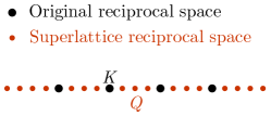
| (29) |
where with are the inequivalent wave vectors in the reciprocal lattice of the original lattice (see the 1d case shown in Fig. 8). Then we can perform the -summation in Eq. (28) to have,
| (30) |
where we have used the fact that is invariant under the shift by a superlattice reciprocal lattice vector .
The translation invariant approximation for the Green’s function on the original lattice is obtained when , i.e. . Therefore, the Green’s function becomes,
| (31) |
Now we just need to calculate using cluster perturbation. The idea is to treat hopping between clusters as perturbation when consider strong on-site interactions. In particular,
| (32) |
where contains intra-cluster terms and contains inter-cluster hopping. Considering nearest-neighbor hopping between the square clusters used in the main text. The cluster construction is reproduced in Fig. 9 with the 4 sites in each cluster labeled by . The hopping matrix is given by (setting lattice constant )
| (33) |
Fourier transforming into the superlattice reciprocal space, we have
| (34) |
which is the form presented in Eq. (17) in the main text. Then the interacting Green’s function is given by
| (35) |
where is the intra-cluster Green’s function that can be easily obtained by exact diagonalization as long as the cluster size is not too big. The obtained can now be plugged into Eq. (31) to calculate the CPT Green’s function for the interacting system.