Atom-field dynamics in curved spacetime

Abstract

Some aspects of atom-field interactions in curved spacetime are reviewed. Of great interest are radiative processes arising out of Rindler and black hole spacetimes, which involve the role of Hawking-Unruh effect. The conventional understandings of atomic radiative transitions and energy level shifts are reassessed in curved spacetime. On one hand, the study of the role played by spacetime curvature in quantum radiative phenomena has implications for fundamental physics, notably the gravity-quantum interface. In particular, one examines the viability of Equivalence Principle, which is at the heart of Einstein’s general theory of relativity. On the other hand, it can be instructive for manipulating quantum information and light propagation in arbitrary geometries. Some issues related to nonthermal effects of acceleration are also discussed.

I Introduction

Quantum optics has witnessed great progress in the past decades, which opened windows to the development of many ground-breaking theoretical tools and unprecedented experimental techniques, having great bearing on fundamental physics and various technological applications. Some prominent advancements include ultraintense laser systems Mourou et al. (2006), cavity QED Walther et al. (2006), techniques ushering to novel quantum phases and phenomena arising out of strong atom-photon interactions Chang et al. (2018), topological photonics Ozawa et al. (2019), gravitational wave interferometry Harry and (forthe LIGO Scientific Collaboration); Aso et al. (2013); Dooley et al. (2016); Yu et al. (2020); Acernese et al. (2020), atom interferometric precision tests for general relativity and gravity Safronova et al. (2018), to name a few of the recent ones. While conventional quantum optical processes are based on flat background space(-time) with an inertial description, recent years have seen intense efforts in understanding the impact of curved background geometry on the optical phenomena, either in classical regime Schultheiss et al. (2010, 2020), helping emulate general relativity and black hole effects in optical structures Leonhardt and Philbin (2006); Philbin et al. (2008); Bekenstein et al. (2016); Patsyk et al. (2018) and analogue spacetime models Faccio et al. (2013); Viermann et al. (2022), or in quantum regime within accelerated frames and curved geometries Lopp et al. (2018a); Scully et al. (2018); Martín-Martínez et al. (2020); Zhang et al. (2014). The motivation for pursuing these directions is manifold. Firstly, one expects achieving possible ways to create test beds for probing cutting edge theoretical problems in fundamental physics that arise in non-Euclidean geometry which, among many include, for example, issues related to quantum gravity Boettcher et al. (2020); Garcia et al. (2020), Hawking-Unruh radiation Steinhauer (2016); Leonhardt (2018); Hu et al. (2019); Sheng et al. (2021), cosmological expansion and particle creation Parker (1969, 1971, 2012); Eckel et al. (2018); Schmit et al. (2020), which are otherwise notoriously difficult to observe. Secondly, these efforts could be potentially helpful in designing novel structures that may manipulate and control light propagation in arbitrary surfaces and complex media. It could also boost the progress in quantum computation and information phenomena by incorporating the effects of acceleration and curvature, which has been actively pursued for last two decades or so Alsing and Milburn (2003); Fuentes-Schuller and Mann (2005a); Downes et al. (2011), paving way for a rapidly developing field of relativistic quantum informationPeres and Terno (2004); Mann and Ralph (2012). It has also sparked intense debates about the role of acceleration in quantum information processes Alsing et al. (2006); Wang and Jing (2011); Friis et al. (2012); Bruschi et al. (2013); Liu et al. (2022) and quantum optical phenomena Lopp et al. (2018b); Martín-Martínez et al. (2020). Similar ideas have also been explored to quantify the role of gravity in the dynamics of Bose-Einstein condensates Sabin et al. (2014); Rätzel et al. (2018a); Schützhold (2018); Howl et al. (2018) and Dirac equation Collas and Klein (2019).

Quantum optical phenomena are deeply grounded in theory of light-matter interactions, or atom-field dynamics Scully and Zubairy (1997); Compagno et al. (1995) that occur in flat spacetime. Many novel phenomena emerge when a transition is made to curved geometries. On a thorough survey of literature, it turns out that there many ways to go forward.

One major line of investigation is to include the contributions from acceleration radiation or celebrated Unruh effect Unruh (1976), also known as Fulling-Davies-Unruh effect Fulling (1973); Davies (1975); Crispino et al. (2008), which posits that a Minkowski vacuum appears as a thermal state to an accelerating observer (Rindler observer), and alludes to the idea that radiation is not a local covariant phenomenon Rohrlich (1961, 1961); Boulware (1980). Likewise, we have contributions from Hawking effect Hawking (1975), which is the thermal radiation detected by a static observer (e.g. an atom) in a black hole geometry. Both of these effects exploit causal horizons of spacetime and use same procedures for the description of quantum fields on curved spacetime Frodden and Valdés (2018). It is expected that when atoms and fields undergo acceleration in Rindler and curved spacetimes, Hawking-Unruh effect does contribute to the atomic transition and energy level shift phenomena. Being concerned with the vacuum physics, this naturally connects Hawking-Unruh effect with the particle creation in quantum vacuum via Casimir Casimir (1948); Bordag et al. (2009) or dynamical Casimir effect Moore (2003); Dodonov (2020), and moving mirror models Scully et al. (2018); Fulling and Davies (1976); Davies and Fulling (1977); Anderson et al. (2017); Good et al. (2017); Belyanin et al. (2006); Scully (2019); Lock and Fuentes (2017). In the past three decades, this has been thoroughly worked out and forms the thrust of this review.

We also make a brief mention of few other directions that seek to introduce curved geometry in the description of quantum systems. Since the seminal work by Chandrasekhar on solving Dirac equation in a Kerr spacetime Chandrasekhar (1976), this has flourished into a major activity of analyzing influence of curved spacetime on quantum mechanical behavior of particles Carter and McLenaghan (1979); Shishkin (1991); Finster and Reintjes (2009); Collas and Klein (2018). In a series of papers by Parker Parker (1980a, 1981a, b, 1981b), the possibility of using atoms as probe of classical spacetime geometry was considered, where the spacetime curvature manifests itself in the atomic spectrum, having dependencies on Ricci curvature. This has spread in a flurry of research activities and extended to many systems (see e.g. Pinto (1993); Parker et al. (1997); de A. Marques and Bezerra (2002); Zhao et al. (2007); Carvalho et al. (2011); Roura (2021).

Other considerations are based on a geometric approach applied to quantum mechanics Caianiello (1981), the maximal acceleration hypothesis and its connection to Lamb shift Lambiase et al. (1998) and Unruh effect (see Benedetto and Feoli (2015) and the relevant references therein). Furthermore, many efforts have been devoted to the study of emissionHiguchi et al. (1997), scattering Crispino et al. (2009) and absorption Macedo et al. (2013); Cardoso and Vicente (2019) of electromagnetic and other fields near black holes, which find connections to black hole superradianceBrito et al. (2015) and probing black hole geometries Bambi (2017). However, this later field-geometry coupling is a much bigger paradigm that extends beyond the scope of present discussion.

By introducing acceleration or spacetime curvature in optical phenomena, it necessarily involves tools from quantum field theory and differential geometry, these studies somehow lie at the boundary between quantum optics and gravity. Though the topics have sparsely been covered in some reviews Crispino et al. (2008); Dodonov (2020); Passante (2018), we believe a comprehensive and detailed review, that could assemble all relevant works in one piece and provide a thorough introduction to this emerging field, is still lacking at the moment. By focusing on atom-field dynamics in curved geometries, we thus hope this short review provides a glimpse of this area and thus becomes handy for beginners. We organize the work as follows.
In Sec. II, we introduce the necessary mathematical tools including Rindler motion and techniques for quantizing fields in curved geometries. This is essential for description of Hawking-Unruh effects and is needed in subsequent discussions. Sec. III is devoted to atomic radiative transition processes and Lamb shift in Rindler and black hole spacetimes, followed by discussions on dispersion and resonant interactions in curved spacetimes. In Sec. IV, we discuss some aspects of particle and energy production in moving mirror models, followed by atom-mirror systems in black hole spacetime. Conclusions are drawn in Sec. V.

II Field quantization in curved spacetime and Hawking-Unruh Effect

II.1 Accelerated observers in flat spacetime: Rindler motion

We begin from Minkowski spacetime metric

$$ds^{2}=c^{2}dt^{2}-dx^{2}-dy^{2}-dz^{2},$$ (1)

which characterizes a four-dimensional continuous spacetime and is an invariant quantity under Lorentz transformation. It represents a non-Euclidean geometry, and sometimes also known as pseudo-Euclidean spacetime. However, for a constant $t$, spatial part of the geometry remains Euclidean Hobson et al. (2006). Based on the sign of $ds^{2}$ in (1), the interval can timelike $(ds^{2}>0)$, null or lightlike $(ds^{2}=0)$ and spacelike $(ds^{2}<0)$. Intuitively, one can view this as if a body moving along its trajectory can have three ways to go. In the first case, body is at rest and time flows. So it moves in time and does not move in space. Second case would mean that it catches up exactly with ray of light. And in this third case, it moves only in space and not in time, which is impossible. Hence the blue region below the light’s trajectory is not causally connected to the body. The situation is shown in the spacetime diagram of Fig. (1), called lightcone.

Figure 1: Lightcone showing different regions of spacetime. Shaded region pertains to accelerated observer.

Note that the shaded region on left and right side (wedges) of the vertical axis is very important for describing accelerated observers in flat spacetime–helping in the description of Unruh effect. A symbolic way of representing a spacetime metric is signature. For Minkowski spacetime in Eq. (1), it is given by $(+,-,-,-)$. By using indexed coordinates $x^{\mu}(\mu=0,1,2,3)$ such that

$$x^{0}\equiv ct,\ \ x^{1}\equiv x\ \ x^{2}\equiv y,\ \ x^{3}\equiv z.\$$ (2)

The metric (1) can be represented in Einstein summation convention for tensors as

$$ds^{2}=\eta_{\mu\nu}dx^{\mu}dx^{\nu},$$ (3)

where $\eta_{\mu\nu}$ is the Minkowski metric tensor. Closely related to these underlying transformations in spacetime are Lorentz and Poincaré groups. The Lorentz transformation is also sometimes written as Misner et al. (1973) $x^{\prime\mu}=\Lambda^{\mu}_{\nu}x^{\nu}$, where $x^{\nu}$ is any four-vector and $\Lambda$ is the Lorentz tensor. The corresponding group comprises three rotations and three boosts and hence a six parameter (also called generators) group. Its extension by adding four spacetime translations, $x^{\prime\mu}=\Lambda^{\mu}_{\nu}x^{\nu}+a^{\mu}$ ($a^{\mu}$ is a constant tensor) constitutes Poincaré group, which obviously has ten generators in total Weinberg (1972).

The inertial motion in special relativity is very well described by the above considerations and can be found in almost every elementary textbook on relativity. So it gives an impression that only objects in uniform motion can be dealt with special theory of relativity. However, this statement is not quite complete. So then, is it possible to incorporate acceleration in a special relativistic decription of motion? The answer is yes. Such accelerated motion is called Rindler motion. The best possible example is a constantly accelerating rocket in space. Recall that we mentioned in the previous section about the shaded wedges of Minkowski spacetime diagram in Fig. (1) on right and left sides of particle worldline. Rindler motion is very well described in that part of Minkowski spacetime as shown below in Fig. (2).

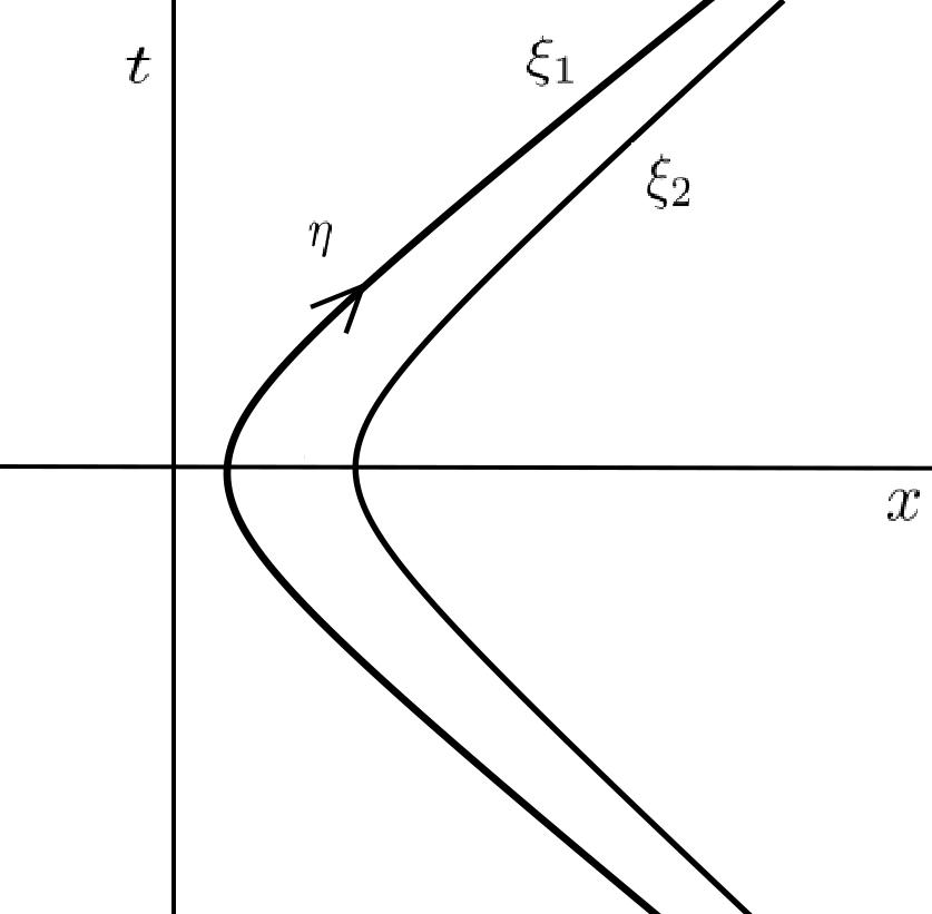
Figure 2: Rindler motion (adopted from E. Frodden et.al Frodden and Valdés (2018)).

In Fig. 2, $t$ and $x$ are time and space coordinates respectively in an inertial reference frame. For simplicity, we only consider motion in right Rindler wedge as shown. We make transformations between an inertial observer and accelerated observer as follows.

Let’s consider an inertial observer $S$ and accelerated observer $B$ having his own frame in which he feels constant acceleration $\alpha$ (his proper acceleration). Also we mark the time of $B$ in his own frame as $\tau$ respectively ($B$’s proper proper time). One can approximate this accelerated motion by considering it as a succession of another inertial frame $S^{\prime}$ (with $t^{\prime}$ as time) having velocity $v$ with respect to $S$. So the accelerated observer is momentarily at rest in $S^{\prime}$. One can easily make a Lorentz transformation between $S$ and $S^{\prime}$ which would be moving at a constant velocity $v$ with respect to $S$ at that particular instant of time. If $S$ measures the acceleration of $B$ as $a$, then acceleration of $B$ in $S^{\prime}$, denoted by $\alpha^{\prime}$ is given by simple transformation of special relativity $a^{\prime}=\gamma^{3}a$, where $\gamma=1/\sqrt{1-v^{/}c^{2}}$ is the usual Lorentz factor. Remember $v$ is the velocity of $S^{\prime}$ w.r.t $S$ at that particular instant of time. Our aim is to get the description of $B$’s own observations in terms of $S$’s. By considering a particular instant of time when $B$ is at rest in $S^{\prime}$, its accelerated is also constant in $S^{\prime}$. At that time,

$$\alpha=\gamma^{3}a=\Bigg{[}\frac{1}{(1-\frac{v^{2}}{c^{2}})}\Bigg{]}^{3}a=\ const.$$ (4)

We can also write the above equation as

$$\alpha=\frac{d}{dt}(\gamma v)=\ const.$$ (5)

By considering the boundary condition $v=0$ at $t=0$, we solve the above equation to get

$$v(t)=\frac{\alpha t}{\sqrt{1+({\alpha t}/c)^{2}}},$$ (6)

and the position $x(t)$ as

$$x(t)=\alpha\int_{0}^{t}\frac{dt^{\prime}}{\sqrt{1+({\alpha t^{\prime}}/c)^{2}}}=\frac{c^{2}}{\alpha}\sqrt{1+({\alpha t}/c)^{2}}.$$ (7)

This gives rise to the following equation of motion

$$x^{2}-t^{2}=\Big{(}\frac{c^{2}}{\alpha}\Big{)}^{2}.$$ (8)

This is clearly an equation of hyperbola. So the worldline of $B$ is a hyperbola as seen from Fig. 2. In terms of proper time $\tau$, we have Socolovsky (2013)

$$t(\tau) =\int_{0}^{t}\sqrt{1-{v(t^{\prime})^{2}}/c^{2}}$$ (9)

$$=\int_{0}^{t}\frac{dt^{\prime}}{\sqrt{1+({at^{\prime}}/c)^{2}}}$$ (10)

$$=\big{(}\frac{c}{\alpha}\big{)}\sinh\Big{(}\frac{\alpha\tau}{c}\Big{)},$$ (11)

and

$$x(\tau)=\Big{(}\frac{c^{2}}{\alpha}\Big{)}\cosh\Big{(}\frac{\alpha\tau}{c}\Big{)}.$$ (12)

In natural units, $c=1$, we have

$$t(\tau)=\frac{1}{\alpha}\sinh\Big{(}\alpha\tau\Big{)},\ \ x(\tau)=\frac{1}{\alpha}\cosh\Big{(}\alpha\tau).$$ (13)

This is called the Rindler transformation which connects an inertial and accelerating observer. Here $\alpha$ and $\tau$ are called Rindler acceleration and Rindler time respectively Rindler (1966). From Eqs. (13) and (13), one can easily identify the hyperbolic polar coordinate representation of $x$ and $t$ as follows

$$t=\xi\sinh\eta,\ x=\xi\cosh\eta,$$ (14)

where $\xi=1/\alpha$ and $\eta=\alpha\tau$. These two parameters $\xi$ and $\eta$ are called Rindler coordinates, and this leaves the metric as

$$ds^{2}=\xi^{2}d\eta^{2}-d\xi^{2},$$ (15)

which is called Rindler metric. Rindler metric can be very well used to describe most the physics of uniform gravitational fields where acceleration is constant i.e. weak-field limit of general relativity. By using Eqs. (14) and (15), Rindler line element in $(1+1)$ dimensions can also be written as Rindler (1966)

$$ds^{2}=e^{2\alpha\xi}(d\tau^{2}-d\xi^{2}).$$ (16)

To cover the whole Rindler wedge, we can accommodate many accelerating observers (infinite in principle!) in Rindler formulation with constant accelerations parameterized by $\xi_{1}$ and $\xi_{2}$ as shown in Fig (2). For each observer’s motion, $\xi$ would be constant along the whole trajectory and only $\eta$ would change. A more general transformation would be Frodden and Valdés (2018)

$$t=\frac{1}{\alpha}f(\xi)\sinh(\eta),\ \ x=\frac{1}{\alpha}f(\xi)\cosh(\eta).$$ (17)

where $f(\xi)$ is a function of $\xi$. Since more the acceleration, more the observer gets close to the origin, this hints to take $f(\xi)$ an increasing function. Choosing $f(\xi)=e^{a\xi}$, the above transformation becomes

$$t=\frac{1}{\alpha}e^{\alpha\xi}\sinh(\eta),\ \ x=\frac{1}{\alpha}e^{\alpha\xi}\cosh(\eta),$$ (18)

which are so-called conformal Rindler coordinates Martin-Martinez and Menicucci (2014), and very often used in literature. The above derivation will be very useful in describing Unruh effect, as follows in the subsequent sections.

II.2 Field quantization in curved spacetime

Next, we discuss some results from quantization of fields on curved spacetimes. We begin by Minkowski description of quantum fields and develop the framework for curved cases. The simplest one is to consider a free Klein-Gordon field which possesses zero spin $(s=0)$, hence a scalar field. The flat space metric signature is $(+,-,-,-)$ and we adopt units in $c=\hbar=1$, unless stated otherwise. The detailed method can be found in many textbooks (see for example, Birrell and Davies (1984); Jacobson (2005); Parker and Toms (2009)). In canonical quantization scheme, a scalar Klein-Gordon field $\phi(x^{\mu})$ and its associated momentum $\pi(x^{\mu})$ appear in a Legendre transformation between Hamiltonian density $\mathcal{H}$ and Lagrangian density $\mathcal{L}$

$$\mathcal{H}=\pi\dot{\phi}-\mathcal{L},$$ (19)

which gives the Hamiltonian $H=\int d^{n-1}x\mathcal{H}$ for an $n$-dimensional spacetime. These two are then promoted to field operators $\hat{\phi}$ and $\hat{\pi}$, such that they possess values at each point $x^{\mu}$. For simplicity, we drop the hat symbols on operators. The equal time commutation relations are imposed as

$$[\phi(t,x),\phi(t,y)] =[\pi(t,x),\pi(t,y)]=0,$$ (20)

$$[\phi(t,x),\pi(t,y)] =i\delta^{n-1}(x-y).$$ (21)

Also, the Lagrangian density, which is Lorentz-invariant, is given by

$$\mathcal{L}=\frac{1}{2}\eta^{\mu\nu}\partial_{\mu}\phi\partial_{\nu}\phi-\frac{1}{2}m^{2}\phi^{2},$$ (22)

where $m$ characterizes the field mass. This gives us the Klein-Gordon equation

$$\eta^{\mu\nu}\partial_{\mu}\partial_{\nu}\phi+m^{2}\phi=0,$$ (23)

or

$$(\Box+m^{2})\phi=0,$$ (24)

where $\Box=\eta^{\mu\nu}\partial_{\mu}\partial_{\nu}$. Thus, in a similar way to harmonic oscillator, we expand field $\phi(t,x)$ as follows

$$\phi(t,x)=\int d^{n-1}k\big{[}\hat{a}_{k}\varphi_{k}(t,x)+\hat{a^{\dagger}_{k}}{{\varphi^{*}}_{k}}(t,x)\big{]},$$ (25)

where $\varphi_{k}$ are complete set of solutions to (23) characterized by vector $k$ (assuming $\varphi$ and $\varphi^{*}$ as positive and negative frequency modes respectively), and $\hat{a}_{k}$ and $\hat{a^{\dagger}_{k}}$ are creation and annihilation operators respectively which follow the commutation relations as mentioned before. By considering some explicit solutions to (23) as $\varphi_{k}=A_{k}e^{i(k.x-\omega_{k}t)}$, with $A_{k}$ as some constant, the normalized modes are given by

$$\phi_{k}(x,t)=\frac{1}{\sqrt{2\omega_{k}(2\pi)^{n-1}}}e^{i(k.x-\omega_{k}t)}.$$ (26)

In the above consideration, $\omega_{k}$ is either a positive or negative frequency satisfying the dispersion relation, $\omega_{k}^{2}=k^{2}+m^{2}$. With these things in hand, we can write

$$H=\int d^{n-1}k\big{[}\hat{n}_{k}+\frac{1}{2}\delta^{(n-1)(0)}\big{]},$$ (27)

which makes sure that $H$ be a Hermitian operator such that $\hat{a}_{k}|n_{k}\rangle$ is its eigenstate. This operator $H$ possesses a ground state $|0\rangle$, such that $\forall\ k,\hat{a}_{k}|0\rangle=0$, which is the Fock vacuum. Thus, for Fock vacuum, the average particle number is

$$\langle 0|\hat{n}_{k}|0\rangle=0,\ \forall\ k.$$ (28)

For the foregoing discussion, one important point must be made here. By considering positive frequency modes which are Lorentz-invariant, we can conclude that the definition of vacuum constructed thereby is also Lorentz-invariant. This situation is changed when we consider the background spacetime as curved.

While making transition to curved spacetime, we replace flat signature $\eta_{\mu\nu}$ by more generic signature $g_{\mu\nu}(+,-,-,...,-)$ and the derivative $\partial_{\mu}$ by covariant derivative $\nabla_{\mu}$, which gives the following Lagrangian for scalar field

$$\mathcal{L}=\frac{1}{2}|g|^{1/2}\Big{(}\frac{1}{2}g^{\mu\nu}\partial_{\mu}\phi\partial_{\nu}\phi-\frac{1}{2}m^{2}\phi^{2}\Big{)},$$ (29)

where $g$ is the determinant of metric tensor $g_{\mu\nu}$. It should be mentioned here that there is a possibility of coupling between the scalar field and gravitational background described by Ricci scalar curvature $R$. This results in the following equation for field $\phi$

$$(\nabla^{\mu}\nabla_{\mu}+m^{2}+\lambda R)\phi=0,$$

where $\lambda$ is the coupling constant. We consider the case of minimal coupling where $\lambda=0$, which reduces above equation to

$$(\nabla^{\mu}\nabla_{\mu}+m^{2})\phi=0.$$ (30)

We take a brief pause here and will return to the above result. In what follows, we discuss Klein-Gordon inner product, which is very important to appreciate difference between flat and curved space quantization. Corresponding to the harmonic oscillator case, if a function $f_{A}$ helps to solve the oscillator equation

$$\ddot{x}+\omega^{2}x=0,$$ (31)

by the substitution $\hat{x}=\hat{a}f_{A}(t)+\hat{a^{\dagger}}f_{A}^{*}(t)$, then it is possible to define an inner product on the space of solutions to (31) as

$$\langle f_{A},f_{B}\rangle=\frac{im}{\hbar}\Big{(}f_{A}^{*}\partial_{t}f_{B}-(\partial_{t}f^{*})f_{B}\Big{)},$$ (32)

where $f_{B}$ is just another function like $f_{A}$ and $\partial_{t}=\frac{\partial}{\partial t}$. With this new notation, the anticommutation relation is $\langle f,f\rangle[\hat{a},\hat{a^{\dagger}}]=1$. For flat space field quantization with two solutions $\phi_{1}$ and $\phi_{2}$ corresponding to Eq.(23), we define this inner product as

$$\langle\phi_{1},\phi_{2}\rangle=-i\int_{\Sigma_{t}}d^{n-1}x\Big{(}\phi_{1}\partial_{t}\phi_{2}^{*}-\phi_{2}^{*}\partial_{t}\phi_{1}\Big{)},$$ (33)

where the integral measure is over a constant time hypersurface $\Sigma_{t}$ which represent Cauchy surfaces for Klein-Gordon equation of (23). A Cauchy surface is a closed hypersurface intersected by every timelike curve only once, if the curve is inextendible. A spacetime is globally hyperbolic, if it has a Cauchy surface. Similarly, for the curved spacetime quantization, the inner product is given by

$$\langle\phi_{1}|\phi_{2}\rangle=i\int_{\Sigma}d^{n-1}x\ n^{\mu}\sqrt{\gamma}\Big{(}\phi_{1}^{*}\nabla_{\mu}\phi_{2}-\phi_{2}\nabla_{\mu}\phi_{1}^{*}\Big{)}.$$

Here the integral measure is defined over spacelike hypersurface $\Sigma$ with normal vector $n^{\mu}$ and induced metric $\gamma_{ij}(\gamma)$. Now it is often helpful to consider two modes of positive- and negative-frequency solutions to Eq.(30) forming a complete basis and then expanding the field operator $\phi$ as a combination of these modes. Thus, for a set of modes $f_{i}$ used by an observer, we write

$$\phi=\sum_{i}(\hat{a}_{i}f_{i}+\hat{a}_{i}^{\dagger}f^{*}_{i}),$$ (34)

where $\hat{a}_{i}$ and $\hat{a}_{i}^{\dagger}$ are identified as annihilation and creation operators following the commutation relations

$$[\hat{a}_{i},\hat{a}_{j}]=[\hat{a}_{i}^{\dagger},\hat{a}_{j}^{\dagger}]=[\hat{a}_{i},\hat{a}_{j}^{\dagger}]=0,$$

and corresponding vacuum state is $|0_{f}\rangle$, such that $\hat{a}|0_{f}\rangle=0_{f}$. It is very important to ascribe a timelike Killing vector for flat spacetime quantization such that one is able to classify the solutions in terms of positive- and negative-frequency modes. In curved spacetime, such a Killing vector does not exist generally, hence our procedure for identifying positive- and negative-frequency mode solutions no more works. For the sake of clarity, we consider another set of modes $g_{i}$ with vacuum $0_{g}$ and corresponding annihilation and creation operators $\hat{b}_{i}$ and $\hat{b}_{i}^{\dagger}$ ( following same commutation relations as that of $\hat{a}_{i}$ and $\hat{a}^{\dagger}_{i}$) respectively by another observer such that

$$\phi=\sum_{i}\Big{(}\hat{a}_{i}g_{i}+\hat{a}_{i}^{\dagger}g^{*}_{i}\Big{)}.$$ (35)

It is possible to define a transformation between $f_{i}$ and $g_{i}$ such that

$$g_{i}=\sum_{i}\Big{(}\alpha_{ij}f_{j}+\beta_{ij}f_{j}^{*}\Big{)},\ \ f_{i}=\sum_{j}\Big{(}\alpha^{*}_{ji}g_{j}-\beta_{ji}g^{*}_{j}\Big{)},$$

which characterizes the scenario where one observer expresses his results in terms of other’s basis modes. This is the famous Bogolubov transformation and helps to write transformation between the operators $\hat{a}_{i}$ and $\hat{b}_{i}$ as follows

$$\hat{a}_{i}=\sum_{j}\Big{(}\alpha_{ji}\hat{b}_{j}+\beta^{*}_{ji}\hat{b}^{\dagger}_{j}\Big{)},\ \ \hat{b}_{i}=\sum_{j}\Big{(}\alpha^{*}_{ij}\hat{a}_{j}-\beta^{*}_{ij}\hat{a}^{\dagger}\Big{)},$$ (36)

with $\alpha_{ij}$ and $\beta_{ij}$ as Bogolubov coefficients which follow the orthonormalization relations

$$\sum_{j}\Big{(}\alpha_{ik}\alpha_{jk}^{*}-\beta_{ik}\beta_{jk}^{*}\Big{)} =\delta_{ij},$$

$$\sum_{j}\Big{(}\alpha_{ik}\beta_{jk}-\beta_{ik}\alpha_{jk}\Big{)} =0.$$ (37)

Here comes the crucial step. If an observer sees a field in $f$-vacuum while using $f$-modes, in which case there are no particles, the same system as seen by other observer using $g$-modes would be such that expectation value of $g$-number operator is given by

$$\langle 0_{f}|\hat{n}_{gi}|0_{f}\rangle =\langle 0_{f}|\hat{b}_{i}^{\dagger}\hat{b}_{i}|0_{f}\rangle$$ (38)

$$=\sum_{j}\beta_{ij}\beta^{*}_{ij}$$

$$=\sum_{j}|\beta_{ij}|^{2},$$

while we made use of (36). $\beta_{ij}$ is a non-zero quantity, which clearly manifests that annihilation operator of one observer is a combination of annihilation and creation operators of other one. Eq. (38) signifies a remarkable result. It demonstrates that, while one observer sees field in vacuum state, the same field appears to other observer to be in a non-vacuum state. Thus, the uniqueness of vacuum state in Minkowski spacetime is broken completely in a curved spacetime. It is only for the inertial case, where $\beta_{ij}=0$, that the two observers agree on the definition of vacuum. It is this non-uniqueness of field states between the two observers which leads to the phenomenon of Hawking-Unruh effect.

II.3 Thermality of Minkowski vacuum: Unruh effect

Variously known as Fulling-Davies-Unruh effect or Unruh effect in short, in its simplest form, refers to the detection of thermal radiation by an accelerating observer (Rindler observer) in Minkowski vacuum. Unruh originally discovered it while attempting to understand the underlying mechanism of black hole-originating Hawking radiation Unruh (1976). The mathematical machinery of both these effects is same but the difference lies in the underlying spacetime geometry. While Unruh effect is observed in flat spacetime by an accelerating observer, the underlying spacetime in Hawking radiation is that of a black hole, which obviously is curved. For the derivation, we follow books by Parker and Toms Parker and Toms (2009), and Carroll Carroll (2019).
Recall from the previous section, the Rindler metric in $(1+1)$-dimensions reads (by using (16) and (18))

$$ds^{2}=e^{2\alpha\xi}(-d\tau^{2}+d\xi^{2}).$$ (39)

It is not difficult to recognize that, since metric components in the line element (39) are independent of $\tau$, the vector

$$\partial_{\tau} =\frac{\partial t}{\partial\tau}\partial_{t}+\frac{\partial x}{\partial\tau}\partial_{x}$$

$$=e^{a\xi}\big{[}\cosh(a\tau)\partial_{t}+\sinh(a\tau)\partial_{x}\big{]}$$

$$=a(x\partial_{t}+t\partial_{x}),$$ (40)

is a Killing field associated with the boost in $x$-direction.
The Klein-Gordon equation for a massless particle $[m=0,\ \text{in}\ (\ref{BOXEQN})]$ in Rindler metric of (39) can be expressed as

$$\Box\phi=e^{-2\alpha\xi}(-\partial_{\tau}^{2}+\partial_{\xi}^{2}).$$ (41)

Solving this equation leads us to consider two sets of normalized plane waves corresponding to left and right Rindler wedges respectively

$$g_{k}^{(1)}=\frac{1}{\sqrt{4\pi\omega}}e^{-i(\omega\tau-k\xi)},\ g_{k}^{(2)}=\frac{1}{\sqrt{4\pi\omega}}e^{i(\omega\tau+k\xi)},$$ (42)

Here, we are considering Minkowski and Rindler observers for the description of Unruh effect. For Minkowski observer, the field $\phi$ can be expressed in terms of his choice of annihilation and creation operators ($\hat{a}_{k}$ and $\hat{a}_{k}^{\dagger}$ respectively) as

$$\phi=\int dk\big{(}\hat{a}_{k}f_{k}+\hat{a}_{k}^{\dagger}f_{k}^{*}\big{)},$$ (43)

where $f_{k}$ are the Minkowski plane wave modes. For the Rindler observer with $\hat{b}_{k}$ and $\hat{b}_{k}^{\dagger}$ as annihilation and creation operators respectively, the same reads as

$$\phi=\int dk\Big{(}\hat{b}_{k}^{(1)}g_{k}^{(1)}+\hat{b}_{k}^{(1)\dagger}g_{k}^{(1)*}+\hat{b}_{k}^{(2)}g_{k}^{(2)}+\hat{b}_{k}^{(2)\dagger}g_{k}^{(2)*}\Big{)}.$$

Minkowski vacuum represented by $|0_{M}\rangle$ is defined here as follows

$$\hat{a}_{k}|0_{M}\rangle=0,$$ (44)

and the Rindler vacuum as

$$\hat{b}_{k}^{(1)}|0_{R}\rangle=\hat{b}_{k}^{(2)}|0_{R}\rangle=0.$$ (45)

We emphasize here that, even though the Hilbert space for the theory is same for both observers, they however differ in Fock space description. This is because Rindler vacuum can be described as many-particle state in Minkowski representation, which arises due to fact that a Rindler mode can be written as an admixture of creation and annihilation operators of Minkowski representation. As part of the ansatz outlined in the previous section, we need to compute Bogolubov coefficients that relates Minkowski and Rindler description of the field. For a consistent formulation of field mode description in Rindler frame, we need to define a new set of functions comprising positive and negative frequency modes as

$$h_{k}^{(1)}=\frac{1}{\sqrt{2\sinh(\frac{\pi\omega}{\alpha})}}\Big{(}e^{\pi\omega/2\alpha}g_{k}^{(1)}+e^{-\pi\omega/2\alpha}g_{-k}^{(2)*}\Big{)},$$

and

$$h_{k}^{(2)}=\frac{1}{\sqrt{2\sinh(\frac{\pi\omega}{\alpha})}}\Big{(}e^{\pi\omega/2\alpha}g_{k}^{(2)}+e^{-\pi\omega/2\alpha}g_{-k}^{(1)*}\Big{)},$$

with the inner product $\Big{(}h_{1}^{(1)},h_{k}^{(2)}\Big{)}=\delta(k_{1}-k_{2})$. Also,by employing $h_{k}$ modes, positive and negative frequency Minkowski modes have associated annihilation and creation operators, respectively, such that $\forall k$

$$\hat{c}_{k}^{(1)}|0_{M}\rangle=\hat{c}_{k}^{(2)}|0_{M}\rangle=0,$$

which indicates a description of Minkowski vacuum using $h_{k}$ modes. With these new modes, we write field as

$$\phi=\int dk\Big{(}\hat{c}_{k}^{(1)}h_{k}^{(1)}+\hat{c}_{k}^{(1)\dagger}h_{k}^{(1)*}+\hat{c}_{k}^{(2)}h_{k}^{(2)}+\hat{c}_{k}^{(2)\dagger}h_{k}^{(2)*}\Big{)}.$$

Now, the Rindler annihilation operators $\hat{b}_{k}$’s can be written in terms of $\hat{c}_{k}$’s as

$$\hat{b}_{k}^{(1)}=\frac{1}{\sqrt{2\sinh(\frac{\pi\omega}{\alpha})}}\Big{(}e^{\pi\omega/2\alpha}\hat{c}_{k}^{(1)}+e^{-\pi\omega/2\alpha}\hat{c}_{-k}^{(2)\dagger}\Big{)}.$$ (46)

Similarly, we have

$$\hat{b}_{k}^{(2)}=\frac{1}{\sqrt{2\sinh(\frac{\pi\omega}{\alpha})}}\Big{(}e^{\pi\omega/2\alpha}\hat{c}_{k}^{(2)}+e^{-\pi\omega/2\alpha}\hat{c}_{-k}^{(1)\dagger}\Big{)}.$$ (47)

By making use of (46) and (47), one is able to construct number operator for Rindler observer in terms of $\hat{c}_{k}$’s, which for region I is

$$\hat{n_{R}}^{(1)}(k)=\hat{b}_{1}^{(1)\dagger}\hat{b}_{k}^{(1)}.$$ (48)

Our aim is to compute the particle number in Rindler frame using Minkowski modes. Hence, we have

$$\langle 0_{M}|\hat{n_{R}}^{(1)}(k)|0_{M}\rangle=\langle\hat{b}_{1}^{(1)\dagger}\hat{b}_{k}^{(1)}|0_{M}\rangle.$$

Following (46) and (47), we get

$$\langle 0_{M}|\hat{n_{R}}^{(1)}(k)|0_{M}\rangle =\frac{1}{2\sinh(\frac{\pi\omega}{\alpha})}\langle 0_{M}|e^{-\pi\omega/\alpha}\hat{c}_{-k}^{(1)}\hat{c}_{-k}^{(1)\dagger}|0_{M}\rangle$$

$$=\frac{e^{-\pi\omega/\alpha}}{2\sinh(\frac{\pi\omega}{\alpha})}\delta(0)$$

$$=\frac{1}{e^{2\pi\omega/\alpha}-1}\delta(0).$$ (49)

Here the factor $\delta(0)$ arises out of the use of non-square-integrable plave wave modes. In fact, it is the expectation value of particle number

$$\langle 0_{M}|\hat{c}_{-k}^{(1)}\hat{c}_{-k}^{(1)\dagger}|0_{M}\rangle=\delta(0),$$ (50)

indicating that $\hat{c}_{-k}^{(1)\dagger}|0_{M}\rangle$ is a normalized one-particle state. Eq. (49) shows that Minkowski vacuum looks to the Rindler observer like a thermal state with non-zero particle content. This makes notion of vacuum and particle frame-dependent in curved spacetime, which means that they do not represent some fundamental elements in non-inertial frames. It is thus argued that this thermal nature of vaccum in the form of Unruh effect is necessary for the consistency of quantum field theory and needs no more experimental verification than the field theory itself Crispino et al. (2008). Finally, taking a look at Eq. (49) shows that this is a Planck spectrum with a characteristic temperature

$$T_{U}=\frac{\alpha}{2\pi},$$

which upon putting the constants back furnishes

$$T_{U}=\frac{\hbar\alpha}{2\pi ck_{B}},$$ (51)

which is the famous relation for Unruh temperature. The weakness of Unruh effect can be readily seen from above relation. To get a feel of it, one can put the value of constants in (51) and this gives an estimate of required acceleration as $10^{20}m/s^{2}$, which is incredibly large. This makes Unruh effect very difficult to observe in the lab. However, some simulation experiments have revealed the consistency of Unruh’s prediction (see Hu et al. (2019) as a most recent work).

II.4 Black holes aren’t black: Hawking radiation

Though Hawking effect bears close similarity to Unruh effect in the mathematical formulation, they only differ in underlying spacetime. Unruh effect occurs in accelerated frames in Minkowski spacetime, while Hawking effect occurs for accelerated observers in curved spacetime. Einstein’s equivalence principle guarantees their consistency. Since the original derivation by Hawking is tedious, so we follow simpler and brief approach by Jacobson Jacobson (2005) and Caroll Carroll (2019).

We write down the Schwarzschild metric of a black hole as

$$ds^{2}=-(1-\frac{2GM}{r})dt^{2}+\frac{1}{(1-\frac{2GM}{r})}dr^{2}+r^{2}d\Omega^{2},$$

where $2GM=R_{S}$ is the Schwarzschild radius. In Schwarzschild spacetime, given an observer with four acceleration $U^{\mu}$, we define a Killing field $K^{\mu}=V(x)U^{\mu}$, such that its magnitude given by

$$V=\sqrt{-K_{\mu}K^{\nu}},$$

which interestingly gives us a redshift factor $V$, that relates the emitted and observed frequency of photons by static observers as $E=-p_{\mu}U^{\mu}$. An observer at a distance $r$ from the black hole such that $r>2GM$, has a geodesic with timelike Killing vector $\partial_{t}$ such that

$$V=\sqrt{1-\frac{2GM}{r}}.$$ (52)

For this observer, the magnitude of four-acceleration is given by

$$\alpha=\frac{GM}{r\sqrt{r-2GM}}.$$ (53)

To put the things in perspective, we consider two observers here, one close to event horizon at a distance $r_{1}>2GM$ and other far away at distance $r_{2}>>2GM$. Now, evidently for the one near the horizon, acceleration is very large, i.e

$$\alpha_{1}>>\frac{1}{2GM}.$$ (54)

Therefore, this much of acceleration sets a time and length scales such that the spacetime looks essentially flat. Here, for a (third) freely-falling observer, nothing unusual happens (see also the associated "firewall" argument Almheiri et al. (2013) or "fuzzball" scenario Mathur (2009)), which implies that the falling observer sees a vacuum state field as Minkowski vacuum, which to the observer at $r_{1}$ distance produces an Unruh effect with radiation having temperature

$$T_{1}=\frac{\alpha_{1}}{2\pi}.$$ (55)

Now, for the observer far away from the black hole at $r_{2}$ distance (in principle $r_{2}\rightarrow\infty$), length and time scales set by the acceleration $\alpha_{2}^{-1}>>2GM$ are large and thus one can not ignore the curvature effects. The overall impact of this curvature is the redshift of radiation frequency that comes from the black hole with the temperature

$$T_{2}=\frac{V_{1}}{V_{2}}\frac{\alpha_{1}}{2\pi}.$$ (56)

One can readily see from (52), as $r_{2}\rightarrow\infty$, $V_{1}\rightarrow 1$, (56) yields

$$T=\lim_{r_{1}\rightarrow 2GM}\frac{V_{1}\alpha_{1}}{2\pi}.$$ (57)

In general, for a black hole, one can write

$$T_{H}=\frac{\kappa}{2\pi}=\frac{\hbar\kappa}{2\pi},$$ (58)

where $\kappa=\lim(V\alpha)$ represents the surface gravity of the black hole. Eq. (58) is the celebrated Hawking effect with $T_{H}$ as Hawking temperature–the observed temperature of the thermal radiation felt by static observer at a far off distance from black hole–Schwarzschild observer.

III Radiative atoms in Rindler and black hole spacetimes

Having discussed the prerequisites, we now discuss atom-field interactions in Rindler and black hole spacetimes, with contributions from Hawking-Unruh effect.

III.1 Unruh thermality in atomic spectrum

Spontaneous excitation of atoms is one of the foremost phenomenon that captures the physics of atom-field interactions. It drives its origin from zero point fluctuations of electromagnetic field Lamb and Retherford (1947); Welton (1948), or the QED radiative reactions for atomic transition frequencies Ackerhalt et al. (1973), or the combination of them Milonni et al. (1973). We consider a field here that is decomposed in terms of creation and annihilation operators

$$\phi(x,t)=\int d^{3}k\ g_{k}[a_{k}(t)e^{ikx}+a_{k}^{\dagger}(t)e^{-ikx}],$$

where $g_{k}=[2\omega_{k}(2\pi)^{3}]^{-1/2}$, that interacts with an atom moving in Minkowski spacetime along the worldline $x(\tau)$. Here, $k$ is the wave vector of the field with the frequency $\omega_{k}$, and $\tau$ is the proper time of the atom. The Hamiltonian for atom-field interaction in the atom’s proper frame is given by

$$H(\tau)=\mu\sigma(\tau)\phi(x(\tau)).$$ (59)

Here $\mu$ is the atom-field coupling constant, and $\sigma(\tau)$ is the atomic lowering operator. As a part of the standard solution procedure for Heisenberg equations of motion, field $\phi$ in the interaction (59) is split into free and source parts Audretsch and Müller (1994)

$$\phi^{f}(x(\tau)) =\int d^{3}k\ g_{k}[a_{k}(0)e^{i(kx-\omega_{k}t)}$$ (60)

$$+a_{k}^{\dagger}(0)e^{-i(kx-\omega_{k}t)}],$$

and

$$\phi^{s}(x(\tau))=i\mu\int_{\tau_{0}}^{\tau}d\tau^{\prime}\sigma^{f}(\tau^{\prime})[\phi^{f}(x(\tau^{\prime})),\phi^{f}(x(\tau))],$$ (61)

respectively. Next, an atomic observable $O(\tau)$ is defined, for which the Heisenberg equation of motion

$$\frac{dO(\tau)}{d\tau}=i[H(\tau),O(\tau)],$$ (62)

yields

$$\frac{dO(\tau)}{d\tau}=i\mu\phi(x(\tau))[\sigma(\tau),O(\tau)].$$ (63)

To account for contributions of vacuum fluctuations and radiation reaction for atom excitation, Dalibard, Dupont-Roc and Cohen-Tannoudji (DDC) Dalibard, J. et al. (1982, 1984) proposed that a preferred symmetric ordering between field operator and atomic observable in (63) leads to a meaningful physical description of radiation reaction and vacuum fluctuations. This consideration leads to the following two equations

$$\Big{[}\frac{dO(\tau)}{d\tau}\Big{]}_{VF}=\frac{1}{2}i\mu\phi^{f}(x(\tau))[\sigma(\tau),O(\tau)]$$

$$+\Big{[}\sigma(\tau),O(\tau)\Big{]}\phi^{f}(x(\tau)),$$ (64)

which pertains to $\phi^{f}$, the free part of the field, and

$$\Big{[}\frac{dO(\tau)}{d\tau}\Big{]}_{RR}=\frac{1}{2}i\mu\phi^{s}(x(\tau))[\sigma(\tau),O(\tau)]$$

$$+\Big{[}\sigma(\tau),O(\tau)\Big{]}\phi^{s}(x(\tau)),$$ (65)

which pertains to $\phi^{s}$, the source part of it.

With regard to Unruh effect, an atom is a typical example of point-like Unruh-DeWitt detector Hawking and Israel (2010) that provides means to probe the Unruh thermality of vacuum. In our case, the accelerated atom has observable its Hamiltonian, $H_{A}$, and we consider its interaction with a scalar field. It is found that the rate at which the total energy of the atom with two given states $(|a\rangle$ and $|b\rangle)$ changes is given by adding (64) and (65), which yields

$$\Big{\langle}\frac{dH_{A}}{d\tau}\Big{\rangle}_{tot} =\frac{\mu^{2}}{2\pi}\Bigg{[}-\sum_{\omega_{a}>\omega_{b}}\omega_{ab}^{2}|\langle a|\sigma^{f}(0)|b|\rangle|^{2}$$

$$\times\Bigg{(}1+\frac{1}{e^{2\pi\omega_{ab}/\alpha}-1}\Bigg{)}+\sum_{\omega_{a}<\omega_{b}}\omega_{ab}^{2}|\langle a|\sigma^{f}(0)|b|\rangle|^{2}$$

$$\times\Bigg{(}\frac{1}{e^{2\pi\omega_{ab}/\alpha}-1}\Bigg{)}\Bigg{]},$$ (66)

where $\omega_{ab}=\omega_{a}-\omega_{b}$ is the transition frequency of the atom Audretsch and Müller (1994). From the relation (66), one can see that if the atom is initially in excited state, the term $\omega_{a}>\omega_{b}$ contributes only, leading to spontaneous emission. On the other hand, if the atom is initially in the ground state, the term $\omega_{a}<\omega_{b}$ contributes, which indicates that there is no balance between vacuum fluctuations and radiation reaction, leading to spontaneous excitation of atom even in vacuum. Note the acceleration ($\alpha$) dependence of the energy rate change, which in the limit $\alpha\rightarrow 0$ agrees with that of inertial case. The above result shows a complete conformity with Unruh effect for a scalar field Unruh (1976). In contrast to scalar field, an electromagnetic field interacting with a hydrogen atom, a nonthermal parameter in the form extra factor of $\alpha^{2}$ appears on the R.H.S of (66), which alludes the loss of equivalence between uniform acceleration and thermality, and also affects the contribution of radiation reaction to the atomic energy change for linear acceleration case Zhu et al. (2006) as well as circularly accelerated atom Chen et al. (2015). It turns out that, this thermality of Minkowski vacuum is a must for the consistency of inertial perspective which has been vindicated from the perspective of a co-accelerated observer as well, both with and without boundary Zhou (2016). For Dirac field, by considering a non-linear coupling case, a cross term appears in the rate of mean energy change given by Zhou and Yu (2012a).

$$\Big{\langle}\frac{dH_{A}}{d\tau}\Big{\rangle}_{tot} =-\frac{\mu^{2}}{60\pi^{3}}\sum_{\omega_{a}>\omega_{b}}\omega_{ab}^{6}|\langle a|\sigma^{f}(0)|b|\rangle|^{2}$$

$$\times\Bigg{(}1+\frac{5\alpha^{2}}{\omega_{ab}^{2}}+\frac{4\alpha^{4}}{\omega_{ab}^{4}}\Bigg{)}\Bigg{(}1+\frac{1}{e^{2\pi\omega_{ab}/\alpha}-1}\Bigg{)}$$

$$+\frac{\mu^{2}}{60\pi^{3}}\sum_{\omega_{a}<\omega_{b}}\omega_{ab}^{2}|\langle a|\sigma^{f}(0)|b|\rangle|^{2}$$

$$\times\Bigg{(}1+\frac{5\alpha^{2}}{\omega_{ab}^{2}}+\frac{4\alpha^{4}}{\omega_{ab}^{4}}\Bigg{)}\Bigg{(}\frac{1}{e^{2\pi\omega_{ab}/\alpha}-1}\Bigg{)}.$$ (67)

Though this response of the atom with Dirac field consistent with typical Dirac particle detector Langlois (2006), however the additional term $\alpha^{4}$ in Eq. (67) is absent both in case of scalar and electromagnetic fields, and the contribution of $\alpha^{4}$ term becomes very dominant for $\alpha>>\omega$ Zhou and Yu (2012a), where $\omega$ is the transition frequency of hydrogen atom. A more comprehensive way is to consider Einstein coefficients, since they are a must for understanding these spontaneous transition processes of atoms. In the accelerated atom case, corresponding to ground state $1$ and an excited state $2$, we find spontaneous emission to be enhanced by a thermal factor as

$$A_{21}=\frac{\mu^{2}}{8\pi}\omega\Big{(}1+\frac{1}{e^{2\pi\omega/\alpha}-1}\Big{)},$$ (68)

compared to the inertial case, $A_{21}=\frac{\mu^{2}}{8\pi}\omega$, while we get a weighted thermal correction to the spontaneous excitation rate

$$A_{12}=\frac{\mu^{2}}{8\pi}\omega\Big{(}\frac{1}{e^{2\pi\omega/\alpha}-1}\Big{)}.$$ (69)

It can be seen that excitation rate given by (69) vanishes as $\alpha\rightarrow 0$ in agreement with Unruh effect Audretsch and Müller (1994) (see also Rizzuto and Spagnolo (2011); Zhang (2016) for the inclusion of a boundary). Interestingly, based on a time-dependent perturbative method, similar results to that of (69) have been obtained in Barton and Calogeracos (2005, 2008); Calogeracos (2016), indicating a great agreement with that of DDC formalism considered here.

Since entanglement is a key ingredient of quantum information, cryptography and computation Raimond et al. (2001), it would be reasonable to study the impact of acceleration on radiative transitions of entangled atoms. Some of important treatments on the subject concerns the link between spontaneous emission and entangled states in Minkowski vacuum Yu and Eberly (2004). Also boundaries have been shown to play decisive role in transition probabilities of entangled atoms Arias et al. (2016); Zhang and Zhou (2019). The issue has also been dealt within DDC formalism as well, with Menezes and Svaiter (2016a) and without accelerationMenezes and Svaiter (2016b) . For the inertial case, both radiation reaction and vacuum fluctuations cancel at asymptotic times, while they are responsible for decay of entanglement between the atoms. This means that entanglement could serve as an interplay between radiation reaction (a classical concept) and vacuum fluctuations (quantum concept) Menezes and Svaiter (2015). It is found that if the acceleration of atoms in this case is very large, the contributions of radiation reaction and vacuum fluctuations are distinct Menezes and Svaiter (2016b), as given by

$$\Bigg{\langle}\frac{dH_{A}}{d\tau}\Bigg{\rangle}_{VF}=\frac{\omega^{4}\mu^{2}}{3\pi}\Bigg{(}\frac{\alpha^{2}}{\omega^{2}}+1\Bigg{)}\Bigg{(}1+\frac{2}{e^{2\pi\omega/\alpha}-1}\Bigg{)},$$ (70)

and

$$\Bigg{\langle}\frac{dH_{A}}{d\tau}\Bigg{\rangle}_{RR}=-\frac{\omega^{4}\mu^{2}}{3\pi}\Bigg{(}\frac{\alpha^{2}}{\omega^{2}}+1\Bigg{)}$$ (71)

which is depicted in Fig. 3.

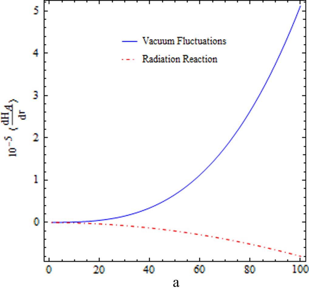
Figure 3: Contributions of vacuum fluctuations (blue solid line) and radiation reaction (red dashed line) for an entangled accelerated two-atom system for the variation of $a$, where $\alpha=ae^{-a\xi}$. The chosen parameters include $\omega=5,\mu=1,\mu^{1}=\mu^{2}=\mu^{3}=1$ and Rindler coordinates $\xi_{1}=\xi_{2}=0$ in natural units ( Menezes et al. Menezes and Svaiter (2016b)).

The situation is further modified if one considers the system interacting with a scalar field near a boundary. By introducing a perfectly reflecting boundary near the entangled system, the transition rates become dependent upon atom-boundary separation, separation between the atoms and the acceleration $\alpha$ Zhang and Zhou (2019). For some cases of radiative processes of entangled atoms, the acceleration produces a nonthermal behaviour in the atomic energy changes and could also possibly pave way for manipulating the radiative behaviour of entangled systems Zhang and Zhou (2019); Zhou and Yu (2020a) (see also Zhou and Yu (2020b) for the case of co-accelerated observer).

Spontaneous transitions are often associated with radiative energy shifts in atoms, which includes Lamb shift. However, there exists a distinction between the behaviour of scalar and electromagnetic fields in contributing to the energy shift Passante (1998); Rizzuto and Spagnolo (2009). Since for inertial case, it is very well known that vacuum fluctuations, and not the radiation reaction, contribute to Lamb shift, it turns out that this situation still holds in accelerated case as well. Once again, consider a uniformly accelerated two-level atom interacting with a massless scalar field which undergoes an energy shift. Since in this case, radiation reaction generally does not contribute anything Audretsch et al. (1995), we have the following contributions to Lamb shift

$$\Delta=\Delta_{0}+\frac{\alpha^{2}\mu^{2}}{192\pi^{2}}\frac{1}{\omega},$$ (72)

where $\Delta_{0}$ is the Lamb shift for inertial case. The extra factor here comes from acceleration and is purely contributed by vacuum fluctuations Audretsch and Müller (1995). For arbitrary stationary spacetimes, we have

$$\Delta=\Delta_{0}+\mathcal{D},$$ (73)

where $\mathcal{D}$ is an extra term that can be evaluated for particular type of acceleration. For the circular acceleration case, the correction term comes out be Audretsch et al. (1995)

$$\mathcal{D} =\frac{\alpha\mu^{2}}{64\sqrt{3}\pi^{2}}\Bigg{[}e^{-2\sqrt{3}B\omega/\alpha}\bar{Ei}\bigg{(}2\sqrt{3}B\frac{\omega}{\alpha}\bigg{)}$$ (74)

$$-e^{2\sqrt{3}B\omega/\alpha}\bar{Ei}\bigg{(}-2\sqrt{3}B\frac{\omega}{\alpha}\bigg{)}\Bigg{]},$$

where $\bar{Ei}$ is the principal value of exponential integral function. Here the factor $B$ is related to Lorentz factor ($v$ is the velocity of atom) as

$$B=1-\frac{1}{5}(v\gamma)^{-2}.$$ (75)

The correction is graphically shown below in Fig. 4 against the inertial emission rate $\Gamma_{inertial}=\mu^{2}\omega/8\pi$

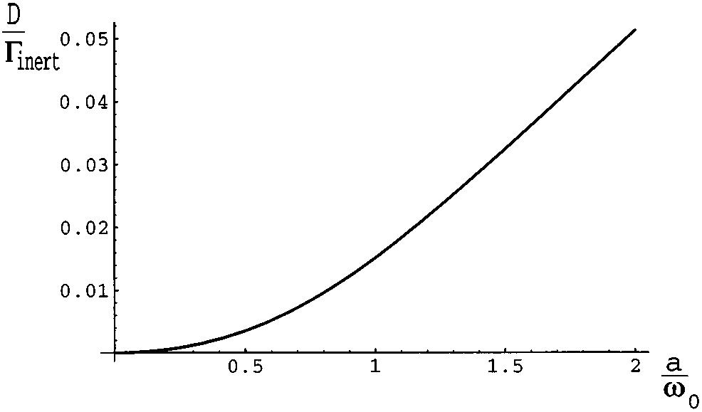
Figure 4: Enhancement of atomic energy shift $\mathcal{D}$ due to acceleration (from Audretsch et al. Audretsch et al. (1995)).

The above plot shows clearly the enhancement of energy shifting compared to the inertial emission rate of the atom. Beyond Unruh contribution, in some multilevel atoms, acceleration can induce Raman-like transitions. By virtue of these transitions, some states show no contribution from Unruh effect due to acceleration Marzlin and Audretsch (1998). It is worthwhile to mention here that the impact of acceleration or gravity on the atomic spectrum and level shifting has been considered in other formalisms as well, quite different from the one considered here. The implication is that gravity plays a great role in quantum phenomena by using atom to probe the spacetime curvature effects Parker (1969); Audretsch and Marzlin (1994). This has been extended to probe various gravity models Olmo (2008); Singh and Mobed (2011); Wong and Davis (2017). Very recently, this line of work also finds connections to some table-top experimental setups with interesting cosmological implications Brax et al. (2018); Sabulsky et al. (2019).

III.2 The case of black holes

III.2.1 Hawking contributions to atomic spectrum

In this section, we discuss the atomic transition processes and energy level shifting occurring in different curved spacetimes of black holes. Since the underlying space is curved, one must expect Hawking radiation to play role , since equivalence principle guarantees the correspondence between Unruh and Hawking effect. But before jumping to the radiative processes, it is necessary to mention the defining properties of black holes. No-hair theorem posits that all black hole solutions of Einstein-Maxwell equations of general relativity are characterized by only three parameters Hobson et al. (2006): Mass ($M$), angular momentum ($J$) and charge $(Q)$, related by

$$M^{2}-\big{(}\frac{J}{M}\big{)}^{2}-Q^{2}\geq 0,$$ (76)

in natural units $c=G=1$. The most general case, when all these three parameters are present, corresponds to Kerr-Newmann black holes (charged, spinning), which reduces to Kerr black hole (uncharged, spinning) for $J\neq 0,Q=0$, Reissner-Nordström black hole (charged, non-spinning) for $J=0,Q\neq 0$ and Schwarzschild (uncharged, non-spinning) black hole for $J=Q=0$. So these parameters are expected to play great role in the atomic radiative phenomena. The choice of vacuum state in a black hole spacetime is also of paramount importance. Contrary to Minkowski spacetime, where vacuum is associated with nonoccupation of positive frequency field modes corresponding to a unique definition of time and time-like Killing vector, no such definition exists in curved spacetime.

One can choose vacuum with respect to Schwarzschild time $t$ i.e. for static observer far from black hole, which happens to be the natural definition of time. For this choice of time, Boulware vacuum is the vacuum state defined with respect to existence of normal modes for Killing vector $\partial/\partial t$, but the expectation value of renormalized stress-energy tensor in freely-falling frame diverges at horizon Sciama et al. (1981). However, this divergence is removed on the future horizon in Unruh vacuum Unruh (1976), which is the most suitable choice of vacuum state of gravitational collapse of a massive body. In Unruh vacuum, the frequency modes coming from past horizon are defined with respect to Kruskal coordinates, the canonical affine parameter at past horizon. In addition to this, Hartle-Hawking vacuum Hartle and Hawking (1976) is not empty at infinity and has rather thermal particles coming from infinity when black hole and thermal radiation are in equilibrium.

The effects of acceleration or curvature on atomic spectrum and radiative phenomena have been dealt in many paradigms. One of the possible ways is to incorporate Maximal Acceleration of Caianiello Papini (2015) into the radiative processes and Lamb shift of atoms. The basic idea is to consider an accelerating atom of mass $m$ following a worldline in the metric

$$\bar{ds}^{2}=g_{\mu\nu}dx^{\mu}dx^{\nu}\Big{[}1-\frac{|\ddot{x}|^{2}}{\mathcal{A}_{m}^{2}}\Big{]},$$ (77)

where $g_{\mu\nu}$ is metric of some background gravitational field, $\ddot{x}^{\mu}$ its acceleration and $\mathcal{A}_{m}=(\frac{2mc^{3}}{\hbar})$ is the maximum acceleration limit. Note that the effective geometry given by (77) is a mass-dependent correction and induces curvature. With that spacetime configuration, the correction to $2S$-$2P$ Lamb shift in hydrogen atom has been demonstrated to be compatible with experiment Lambiase et al. (1998). Many other issues that have been analyzed within this Maximal Accleration model including its relevance to Unruh effect Benedetto and Feoli (2015) and some aspects of radiative phenomena Papini (2015). However, here we continue to discuss the curvature effects on atomic radiative and level shift phenomena using DDC formalism as done in the Rindler case. This will maintain the continuity of our discussion in a natural way.

We begin by highlighting the work by Higuchi et al.Higuchi et al. (1998), who considered the possible excitation and emission processes of a static source outside a Schwarzschild black hole due to Hawking radiation. A point-like detector interacting with a massless scalar field in Unruh vacuum gives the following response rate

$$R_{tot}=\frac{q^{2}\alpha}{4\pi^{2}},$$ (78)

where $q$ is the coupling constant between source and field and $\alpha$ is the proper acceleration of source held fixed in black hole spacetime. In terms of response of static sources, this result establishes an equality between Schwarzschild spacetime (with Unruh vaccum) and Minkowski spacetime (with Minkowski vaccum), which is kind of unexpected result, since all classical formulations of equivalence principle are locally valid, while the quantum states are defined golablly Higuchi et al. (1998). However, no such equality is found for electromagnetic Crispino et al. (2001) and massive scalar fields Castineiras et al. (2003). Using DDC formalism, which is different than one used by Higuchi et al. Higuchi et al. (1998), we discuss spontaneous excitation and Lamb shift of an atom interacting with scalar and electromagentic fields in black hole spacetime. However, it is interesting to see that the essence of both of these approcahes is the vindication of Hawking’s prediction Hawking (1975).

Consider an atom as a point-like detector held static in Schwarzschild black hole spacetime. The metric, in the units $c=\hbar=G=k_{B}=1$, is given by

$$ds^{2} =\Big{(}1-\frac{2M}{r}\Big{)}dt^{2}-\Big{(}1-\frac{2M}{r}\Big{)}^{-1}dr^{2}$$ (79)

$$-r^{2}(d^{2}\theta+\sin^{2}\theta d\phi^{2}),$$

where $M$ is black hole mass and $r$ is the radial distance of atom from black the hole center. For such an atom, we explore how radiation reaction and vacuum fluctuations of massless scalar field contribute to the rate of change of average atomic energy, when the atom-field Hamiltonian in proper frame of atom is $H(\tau)=\mu\sigma(\tau)\phi(x(\tau))$. We discuss the cases for different choices of vacua.

Boulware Vacuum.— For Boulware vacuum, the Wightman function for scalar field is given by Christensen and Fulling (1977); Candelas (1980)

$$D_{B}^{+}(x,x^{\prime}) =\frac{1}{4\pi}\sum_{lm}|Y_{lm}(\theta,\phi)|^{2}$$

$$\times\int_{0}^{+\infty}\frac{d\omega_{k}}{\omega_{k}}e^{-i\Delta t}\big{[}|\overrightarrow{R}_{l}(\omega_{k}|r)|^{2}+|\overleftarrow{R}_{l}(\omega_{k}|r)|^{2}\big{]},$$ (80)

where $Y_{lm}(\theta,\phi)$ are spherical harmonics, $R_{l}(\omega_{k}|r)$’s are radial functions pertaining to solution of Klein-Gordon equation, and $\omega_{k}$ the frequency of the field mode. The corresponding Hadamard function of the field reads as

$$C^{F}(x(\tau),x(\tau^{\prime})) =\frac{1}{8\pi}\sum_{lm}|Y_{lm}(\theta,\phi)|^{2}$$

$$\times\int_{0}^{+\infty}\frac{d\omega_{k}}{\omega_{k}}\bigg{[}e^{\big{(}i\omega_{k}\Delta t/\sqrt{1-2M/r}\big{)}}$$

$$+e^{-\big{(}i\omega\Delta t/\sqrt{1-2M/r}\big{)}}\bigg{]}$$

$$\times\big{[}|\overrightarrow{R}_{l}(\omega_{k}|r)|^{2}+|\overleftarrow{R}_{l}(\omega_{k}|r)|^{2}\big{]},$$ (81)

and the corresponding Pauli-Jordan (or Schwinger) function of the field are

$$\chi^{F}(x(\tau),x(\tau^{\prime})) =\frac{1}{8\pi}\sum_{lm}|Y_{lm}(\theta,\phi)|^{2}$$

$$\times\int_{0}^{+\infty}\frac{d\omega_{k}}{\omega}\bigg{[}e^{\big{(}i\omega_{k}\Delta t/\sqrt{1-2M/r}\big{)}}$$

$$-e^{-\big{(}i\omega_{k}\Delta t/\sqrt{1-2M/r}\big{)}}\bigg{]}$$

$$\times\big{[}|\overrightarrow{R}_{l}(\omega_{k}|r)|^{2}+|\overleftarrow{R}_{l}(\omega_{k}|r)|^{2}\big{]}.$$ (82)

We now make use of (81) and (82) in the equations for vacuum fluction and radiation reaction contributions to atomic energy in DDC formalism Dalibard, J. et al. (1982, 1984); Audretsch and Marzlin (1994), which is given by

$$\Bigg{\langle}\frac{dH_{A}}{d\tau}\Bigg{\rangle}_{VF}=2i\mu^{2}\int_{\tau_{0}}^{\tau}d\tau^{\prime}C^{F}(x(\tau),x(\tau^{\prime}))\frac{d}{d\tau}\chi^{A}(\tau,\tau^{\prime}),$$

and

$$\Bigg{\langle}\frac{dH_{A}}{d\tau}\Bigg{\rangle}_{RR}=2i\mu^{2}\int_{\tau_{0}}^{\tau}d\tau^{\prime}\chi^{F}(x(\tau),x(\tau^{\prime}))\frac{d}{d\tau}C^{A}(\tau,\tau^{\prime}),$$

respectively, to yield the mean rate of change of total atomic energy as Yu and Zhou (2007a); Zhou and Yu (2012b)

$$\Bigg{\langle}\frac{dH_{A}}{d\tau}\Bigg{\rangle}_{tot} =-\frac{\mu^{2}}{2\pi}\sum_{\omega_{a}>\omega_{b}}\omega_{ab}^{2}|\langle a|\sigma^{f}(0)|b\rangle|^{2}$$

$$\times\Big{[}1+\frac{1}{16M^{2}\omega_{ab}^{2}}\sum_{l=0}^{\infty}(2l+1)|B_{l}(0)|^{2}\Big{]},$$ (83)

with $B_{l}(0)$ as reflection coefficient with the property $\overrightarrow{B_{l}}(\omega)=\overleftarrow{B_{l}}(\omega)=B_{l}(\omega)$, while the relation (83) is derived using Regge-Wheeler tortoise coordinates $r_{*}=r+2M\ln(r/2M-1)$. It indicates that in Boulware vacuum, the mean atomic of energy is enhanced compared to Minkowski case and also behaves normally at the horizon which is in sharp contrast to response rate of an Unruh-Dewitt detector Candelas (1980). If one considers electromagnetic field, one must first define a quantization rule before calculating the contribution from the field. Crispino et al. Crispino et al. (2001) have carried out the quantization of electromagnetic field in exterior region of Schwarzschild black hole using Gupta-Bleuler condition in a modified Feynman gauge. This helps one to define correlation functions and vacuum states of the field. In this case, the mean rate of total energy becomes Zhou and Yu (2012b)

$$\Bigg{\langle}\frac{dH_{A}}{d\tau}\Bigg{\rangle}_{tot} =-\frac{\mu^{2}}{3\pi}\sum_{\omega_{a}>\omega_{b}}|\langle a|\sigma^{f}(0)|b\rangle|^{2}\omega_{ab}$$

$$\times\Big{[}1+\frac{\alpha^{2}}{\omega_{ab}^{2}}+f(\omega_{ab},r)\Big{]},$$ (84)

with the proper acceleration

$$\alpha=\frac{M}{r^{2}\sqrt{g_{00}}}=\frac{M}{r^{2}\sqrt{1-2M/r}}.$$ (85)

Thus, it is clear from the Eq. (84), that the response of atom to electromagnetic field is different compared to that of scalar field with the appearance of gray-body factor $f(\omega_{ab},r)$. The energy change rate diverges as the event horizon is reached and approaches zero at asymptotic infinity where the spacetime is flat i.e. $\alpha\rightarrow 0$, while for scalar field, it is finite Yu and Zhou (2007a, b) . This indicates the equivalence of Boulware vacuum for static observer in Schwarzschild spacetime and Rindler vacuum in flat spacetime. For a two-atom system, the mean rate change demonstrates the possibility of generating entanglement between them, even if they are initially prepared in a separable state in Boulware vacuum, which coincides with the conclusion in Cliche and Kempf (2011). This entanglement however degrades if the system is near event horizon Menezes (2016). As acceleration is known to degrade entanglement Fuentes-Schuller and Mann (2005b), this is expected near event horizon, since the acceleration is large when Schwarzschild radius is approached as seen from (85). Thus, for studying entanglement in black hole spacetimes, the consideration of Hawking effect is of paramount importance.

Unruh Vacuum.—

In this case, we first consider the Wightman function as

$$D_{U}^{+}(x,x^{\prime}) =\frac{1}{4\pi}\sum_{lm}|Y_{lm}(\theta,\phi)|^{2}\times$$

$$\int_{-\infty}^{+\infty}\frac{d\omega_{k}}{\omega_{k}}\Bigg{[}\frac{e^{-i\omega_{k}\Delta t}}{1-e^{-2\pi\omega_{k}/\kappa}}|\overrightarrow{R_{l}}(\omega_{k})|^{2}$$

$$+\theta(\omega_{k})e^{-i\omega_{k}\Delta t}\overleftarrow{R_{l}}(\omega_{k})|^{2}\Bigg{]},$$ (86)

which clearly shows how surface gravity of black hole $\kappa$ enters the field quantization. This leads us to the following mean rate of atomic energy change for scalar field case Yu and Zhou (2007a)

$$\Bigg{\langle}\frac{dH_{A}}{d\tau}\Bigg{\rangle}_{tot} =-\frac{\mu^{2}}{3\pi}\sum_{\omega_{a}>\omega_{b}}|\langle a|\sigma^{f}(0)|b\rangle|^{2}\omega_{ab}^{2}$$

$$\times\Bigg{[}\bigg{(}1+\frac{1}{e^{2\pi\omega_{ab/\kappa_{r}}}-1}\bigg{)}\overrightarrow{P}(\omega_{ab})+\overleftarrow{P}(\omega_{ab})\Bigg{]}$$

$$+\frac{\mu^{2}}{3\pi}\sum_{\omega_{a}<\omega_{b}}|\langle a|\sigma^{f}(0)|b\rangle|^{2}\omega_{ab}^{2}\Bigg{[}\frac{P(\omega_{ab})}{e^{2\pi\omega_{ab/\kappa_{r}}}-1}\Bigg{]},$$ (87)

where we have substituted $\kappa_{r}=\kappa/(\sqrt{1-2M/r})$, $\overrightarrow{P}(\omega_{ab})$ and $\overleftarrow{P}(\omega_{ab})$ are factors that arise out radial functions $\overrightarrow{R}_{l}(\omega_{k})$ and $\overleftarrow{R}_{l}(\omega_{k})$ respectively, with $P(\omega_{ab})=\overrightarrow{P}(\omega_{ab})+\overleftarrow{P}(\omega_{ab})$, and this relation is same for electromagnetic case Zhou and Yu (2012b). One can see that in Unruh vacuum, the balance between radiation reaction and vacuum fluctuations is broken and leads to spontaneous excitation of atom due to positive contribution from second term in Eq. (87). Thus, Unruh vacuum tends to destabilize the atom as compared to Boulware case [see Eq.(85)]. In the limiting case of $r\rightarrow 2M$, atom gets some thermal contributions at Tolman temperature, $T=(g_{00})^{-1/2}T_{H}$ ($T_{H}$ is usual Hawking temperature) from black hole appear as seen from (87), while for the case $r\rightarrow\infty$, some thermal contributions occur from the back-scattering of outgoing flux from black hole off the curvature Yu and Zhou (2007a); Zhou and Yu (2012b). For coupled atoms, entanglement can be generated even for asymptotically large $\Delta t$ in contrast to the Boulware vacuum Menezes (2016), where the initial entangled atom state is degraded as the atom approaches event horizon.

Hartle-Hawking Vacuum.— We briefly mention here that in this case, the appearance of thermal contributions from surface gravity via the factors $1/(e^{2\pi\omega_{ab}/k_{r}}-1)$ similar to Unruh vaccum case, tends to increase the atomic energy changes and excitation occurs as if the atom is in a thermal bath at some temperature which tends to approach Hawking temperature in the asymptotically far off distance. Some additional thermal factors in the form of $f(\omega_{ab})$ and quadratic acceleration $\alpha^{2}$ appear in Eq. (87). This makes situation similar to that of electromagnetic field fluctuations in flat space in presence of boundaries Yu et al. (2006). This demonstrates that electromagnetic field fluctuations scatter off the spacetime curvature, as field modes do in flat spacetime Zhou and Yu (2012b). For the entangled case, Hartle-Hawking vacuum has similar behaviour to the Unruh vacuum case Menezes (2016).

Kerr spacetime.— We point out here, that the Schwarzschild geometry is the simplest case of spherically symmetric spacetime. One interesting case would be to consider rotating spacetime of Kerr black holes Visser (2007), which in Boyer-Lindquist coordinates is given by the metric

$$ds^{2} =-\big{(}1-\frac{2Mr}{\rho^{2}}\big{)}dt^{2}-\frac{4Mar\sin^{2}\theta}{\rho^{2}}dtd\phi$$

$$+\frac{\rho^{2}}{\Delta}dr^{2}+\rho^{2}d\theta^{2}+\frac{\sum}{\rho^{2}}\sin^{2}\theta d\phi^{2},$$

where $\rho^{2}=r^{2}+a^{2}\cos^{2}\theta$, $\Delta=r^{2}-2Mr+a^{2}$ and $\sum=(r^{2}+a^{2})^{2}-a^{2}\Delta\sin^{2}\theta$. Such a metric characterizes a stationary and axially symmetric rotating black hole and has two commuting Killing vectors. In this case, some difficulties arise in defining equivalent vacuum state to Hartle-Hawking vacuum Jacobson (1994), and many new vacuum states can be considered, viz. Candelas-Chrzanowski vacuum and Frolov-Thorne vacuum. A noteworthy feature of rotating geometry is its ability to harbour some crucial phenomena like black hole superradiance and energy extraction Brito et al. (2015).

The problem of atom-field interaction in Kerr geometry has been worked by Menezes Menezes (2017). The analysis has indicated that if one considers a static atom in Boulware vacuum, the total rate in energy change is such that a fine tuning exists between vacuum fluctuations and radiation reaction for atom in ground state stablizes it against spontaneous excitation. For an excited atom, they contribute equally to spontaneous excitation. This result is analogous to atom interacting with a quantum field in Minkowski spacetime. Importantly, for asymptotic limit, $r\rightarrow\infty$, decay rate goes arbitrarily high due to occurrence of superradiance Brito et al. (2015).

For Unruh vacuum, the excitation of the atom manifests Hawking effect. For this to occur, the condition to be satisfied is $|(\omega_{ab}/\sqrt{g_{00}})|>m\Omega_{H}$, where $\Omega_{H}$ is black hole angular velocity

$$\Omega_{H}=\frac{a}{r_{+}^{2}+a^{2}},$$ (88)

with $r_{+}=M+\sqrt{M^{2}-a^{2}}$ and $a=J/M$ as black hole parameter and $g_{00}$ is the component of metric tensor. Also, the energy gap between the states and the angular velocity of the black hole have a great role in setting the behaviour of the total energy rate. It has also been shown that the thermal radiation at temperature

$$T=\frac{\kappa_{H}}{2\pi\sqrt{g_{00}}},$$ (89)

allows non-superradiant energy gaps to be spontaneously excited. The Kerr black hole rotation enters the energy rate as chemical potential as expected Birrell and Davies (1984).

For Candelas-Chrzanowski-Howard vacuum state, a thermal contribution for both cases, $|(\omega_{ab}/\sqrt{g_{00}})|>m\Omega_{H}$ and $|(\omega_{ab}/\sqrt{g_{00}})|<m\Omega_{H}$ is verified, unlike Unruh vacuum. For some terms proportional to radial functions, rotation doesn’t affect the rate which means vacuum does not follow the $t-\phi$ reversal symmetry of Kerr geometry.
Other possible candidate for equivalent Hartle-Hawking vacuum for Kerr black hole is Frolov-Thorne vacuum Frolov and Thorne (1989) (The details can be found in Ottewill and Winstanley (2000)). As angular velocity of black hole acts as chemical potential Birrell and Davies (1984), for the atomic transition, it is greater than the energy gap. It is well known that the emission depends upon azimuthal quantum number $m$ with respect to rotation axis through the thermal factor

$$\frac{1}{\exp\Big{[}{\frac{2\pi(\omega_{ab}/\sqrt{g_{00}}-m\Omega_{H})}{\kappa}}\Big{]}-1},$$ (90)

which therefore enhances the excitation probability of the atom if its angular momentum is oriented towards that of the black hole. Furthermore, the limit $M\rightarrow\infty$ corresponds to $T\rightarrow 0$, which produces a negative flux which means black hole stimulates the emission process. This is the very essence of Unruh-Starobinskii effect, the quantum analogue of superradiance Starobinskii (1973); Unruh (1974); Matacz et al. (1993). The case of a stationary atom with a zero angular momentum has also been studied in Menezes (2017). Superradiance also modifies the two-atom entanglement dynamics very significantly compared to Schwarzschild case, if the system is probed via Born-Markov approximation Menezes (2018). For the case of entangled atoms in de Sitter spacetime, the energy variation is dependent on a certain characteristic length scale. If the distance is smaller than this scale, energy change rate is same as that of thermal Minkwski vacuum. Beyond that scale, both spacetimes have distinct behaviour Liu et al. (2018).

III.2.2 Lamb Shift: vacuum fluctuations, not the radiation reaction

We return to Lamb shift and related radiative shifts now, citing some noted results. For the Lamb shift in black hole spacetime, we continue the analysis based upon the DDC formalism, similar to what we did in Rindler case. First, we consider the Schwarzschild metric, where the atom is interacting with a massless scalar field, given by

$$ds^{2} =\Big{(}1-\frac{2M}{r}\Big{)}dt^{2}-\frac{1}{\big{(}1-\frac{2M}{r}\big{)}}dr^{2}$$

$$-r^{2}(d^{2}\theta+\sin^{2}\theta d\phi^{2}).$$

It has been explicitly shown that we get the following total contribution for relative level shift in Boulware vacuum Zhou and Yu (2010a)

$$\Delta_{B} =\frac{\mu^{2}}{16\pi^{2}}\int_{0}^{\infty}d\omega_{k}P\Big{(}\frac{\omega_{k}}{\omega_{k}+\omega}-\frac{\omega_{k}}{\omega_{k}-\omega}\Big{)}$$

$$+\frac{\mu^{2}}{16\pi^{2}}\int_{0}^{\infty}d\omega_{k}P\Big{(}\frac{\omega_{k}}{\omega_{k}+\omega}-\frac{\omega_{k}}{\omega_{k}-\omega}\Big{)}f(\omega_{k},r),$$ (92)

where $\omega$ is energy level difference between levels, $P$ represents principal value, and the grey-body factor is

$$f(r,\omega_{k})=\frac{1}{4r^{2}\omega_{k}^{2}}\sum_{l=0}^{\infty}(2l+1)|P(\sqrt{g_{00}}\omega_{k})|^{2}.$$

In Eq. (92), the first term is just term representing Lamb shift in boundary-less Minkowski spacetime, and second one is a finite correction in flat spacetime with no boundaries. This correction arises due to backscattering of field modes off the spacetime curvature and is analogous to Lamb shift of atom in presence of reflecting boundaries Audretsch et al. (1995); Meschede et al. (1990). In Unruh vacuum, for atom close to event horizon$(r\rightarrow\infty)$, we get corrections as

$$\Delta_{U}=[1+f(r)]\Delta_{M}+\Delta_{T},$$ (93)

where $\Delta_{M}$ is the Minkowski term for shift given by

$$\Delta_{M}=\frac{\mu^{2}}{16\pi^{2}}\int_{0}^{\infty}d\omega_{k}P\Big{(}\frac{\omega_{k}}{\omega_{k}+\omega}-\frac{\omega_{k}}{\omega_{k}-\omega}\Big{)}.$$ (94)

Here, $\Delta_{T}$ is the additional thermal contribution in Unruh vacuum given by

$$\Delta_{T}=\frac{\mu^{2}}{16\pi^{2}}\int_{0}^{\infty}d\omega_{k} P\Big{(}\frac{\omega_{k}}{\omega_{k}+\omega}-\frac{\omega_{k}}{\omega_{k}-\omega}\Big{)}$$

$$\times\Big{(}\frac{1}{e^{2\pi\omega_{k}}/\kappa_{r}-1}\Big{)},$$ (95)

where $\kappa_{r}=\kappa/\sqrt{g_{00}}$. It is clear from the above, that the atom close to event horizon gets correction to Lamb shift as if it immersed in a thermal bath at temperature given by Tolman relation $T=(1/\sqrt{g_{00}})T_{H}$. Now, in the asymptotic limit , $r\rightarrow\infty$, Eq. (93) gets additional factor with $\Delta_{T}$ as

$$\Delta_{U} =[1+f(r)]\Delta_{M}+f(r)\Delta_{T}.$$ (96)

The correction in (96) appears due to backscattering of outgoing thermal flux from event horizon off the curvature of black hole spacetime. Considering same situations in Hartle-Hawking vacuum state,

$$\Delta_{H} =[1+f(r)]\Delta_{M}+[1+f(r)]\Delta_{T},$$ (97)

for the asymptotic limit $r\rightarrow\infty$, which is consistent with the behaviour of Hawking-Hartle vacuum, and

$$\Delta_{H} =[1+f(r)]\Delta_{M}+[1+f(r)]\Delta_{T},$$ (98)

near the event horizon as $r\rightarrow 2M$. In both Unruh and Hartle-Hawking vacuum, thermal term $\Delta_{T}$ is due to the origin of thermal radiation from the horizon, in agreement with Hawking radiation. It is also noteworthy that this thermal term has the form

$$\Delta_{T}=\frac{\mu^{2}\omega}{4\pi^{2}}[1-\gamma+\ln\Big{(}\frac{T}{\omega}\Big{)}+\mathcal{O}(x_{0}^{2})],$$ (99)

where $\gamma=0.577216$ is Euler constant, $x=\omega_{k}/T$ and $x_{0}=\omega/T$. As the temperature increases, thermal contribution to Lamb shift increases logarithmically Zhou and Yu (2010a). Furthermore, in de Sitter spacetime, the overall contribution for static atom is just a thermal contribution of the form similar to that of Unruh and Hawking-Hartle case, but the thermal factor in Eq.(95) includes cosmological constant $\Lambda$ as follows

$$\frac{1}{\exp\big{[}{\frac{{2\pi\sqrt{3}\omega}}{\sqrt{\Lambda}}\big{]}-1}},$$ (100)

while for freely falling atom, the thermality occurs at the Gibbons-Hawking temperature $T_{f}=\frac{\Lambda}{2\sqrt{3}\pi}$ Gibbons and Hawking (1977); Zhou and Yu (2010b). For the observational signatures of black hole-induced corrections to Lamb shift, one can look into Zhou and Yu (2012c). So far, we have dealt with classical geometry of spacetime in all of the above discussion. However, one can see in the literature, these analyses have also been extended to quantum spacetime Cheng et al. (2019) and topological defects Cai and Ren (2019).

III.3 Acceleration with a non-thermal character?

When neutral atoms or molecules interact with a common electromagnetic field, a kind of interaction develops between them. We identify these interactions as dispersion and resonant interactions Salam (2009). While dispersion interactions are generally witnessed between atoms in ground state, resonant interaction generally occurs when one or both of the atoms are in excited state and possesses a long range character. Resonant interaction is also involved in resonant energy transfer in molecules Salam (2008), which has relevance in biological photosynthesis Fassioli and Olaya-Castro (2010) and interaction between macro-molecules Preto and Pettini (2013). For both of these two processes, there is detailed literature available either in books or in review papers, most of which concerns flat spacetime case or inertial atoms; see Galego et al. (2019) for most recent analysis concerning its connection to chemical reactivity of molecules and Fiscelli et al. (2020) for analysis beyond perturbative approximation. For a recent generic account on this topic, we refer the reader to a nice review article by Passante Passante (2018). However, we see though recent years have seen significant activity in extending these phenomena to accelerated frames and curved spacetimes including outer regions of black holes. It is with this motivation that we intend to briefly review these interactions in curved geometries, beginning from dispersion forces followed by resonant interactions. This will also include discussions on nonthermal aspects of Hawking-Unruh effect.

III.3.1 Dispersion Interactions

The general interaction energy of dispersion interaction between two atoms $A$ and $B$ is given by Salam (2009); Andrews et al. (1989)

$$\Delta E =-\frac{\hbar c}{\pi}\int_{0}^{\infty}du\ \alpha_{A}(iu)\ \alpha_{B}(iu)u^{6}\ e^{-2ur}$$

$$\times\Bigg{(}\frac{1}{u^{2}r^{2}}+\frac{3}{u^{3}r^{3}}+\frac{5}{u^{4}r^{4}}+\frac{6}{u^{5}r^{5}}+\frac{3}{u^{6}r^{6}}\Bigg{)},$$ (101)

where $k=iu$ is the imaginary wavenumber, $r=r_{B}-r_{A}$ is the distance between two atoms, $\alpha_{A}$ and $\alpha_{B}$ are polarizabilities of atom $A$ and $B$ respectively. The relation (101) is valid for regions outside the overlap of two wave functions with $r$ having its dependence on relevant atomic transition wavelengths from the ground state, $\lambda_{rg}=2\pi k_{rg}^{-1}$. From (101), one can study two limiting cases. One is the near zone limit, characterized by $r<\lambda_{rg}$

$$\delta E_{near}=-\frac{2}{3}\sum_{ps}\frac{|\mu^{pg}_{A}|^{2}|\mu^{sg}_{B}|^{2}}{E_{sg}+E_{pg}}\frac{1}{r^{6}},$$ (102)

where $p,s$ denote arbitrary atomic states, $g$ unperturbed ground state. Eq.(102) is Van der Waals (nonretarded regime) relation and clearly scales as $1/r^{6}$. Another is the far zone limit, characterized by $r>\lambda_{rg}$

$$\delta E_{far}=-\frac{23\hbar c}{4\pi}\alpha_{A}\alpha_{B}\frac{1}{r^{7}},$$ (103)

which is Casimir-Polder (or retarded) regime of dispersion interaction and scales as $1/r^{7}$ Passante (2018); Casimir and Polder (1948); Babb (2010).

As mentioned earlier, our focus is on acceleration or curved geometry effects on dispersion interactions. It turns out that the contribution from Hawking-Unruh effect has a great role to play. In fact these accelerated dispersion interactions further establish the consistency of predictions made by Hawking-Unruh effect Zhang and Yu (2011, 2013); Noto and Passante (2013). Here, we consider a pair of atoms $A$ and $B$, each with frequency $\omega$, which move with same proper acceleration $\alpha$, having constant distance $r$ between them. Following the procedure in Marino et al. (2014), we get the expression that shows effect of acceleration on near zone limit of dispersion energy as

$$\langle\delta E_{near}\rangle =-\Big{(}1-\frac{4\alpha^{2}t^{2}}{9c^{2}}\Big{)}\frac{3\hbar c}{2\pi r^{6}}\int_{0}^{\infty}\alpha_{A}\alpha_{B}du$$ (104)

$$+\frac{\alpha^{2}t\hbar}{\pi c^{2}r^{5}}\int_{0}^{\infty}\alpha_{A}\alpha_{B}du,$$

which shows that the energy is time $t$ and acceleration $a$ dependent in the form of $1/r^{5}$ term. Compared to inertial case, this additional term decreases slowly with inter-atomic separation $r$. Similarly, for far zone limit , we have

$$\langle\delta E_{far}\rangle =-\frac{\hbar c}{\pi}\frac{\alpha_{A}\alpha_{B}}{r^{7}}\Big{(}\frac{23}{4}-\frac{7\alpha^{2}t^{2}}{24c^{2}}\Big{)}$$ (105)

$$+\frac{11\hbar\alpha^{2}t}{8\pi c^{2}}\frac{\alpha_{A}\alpha_{B}}{r^{6}},$$

which shows that additional contributions from acceleration induce a $1/r^{6}$ behaviour in the energy, which is longer than usual $1/r^{7}$ behaviour in far zone regime for atoms at rest. For this case, if one uses DDC formalism for calculating contributions of vacuum fluctuations assuming a scalar field, the result turns out to yield an acceleration-dependent length scale, $r_{0}$ characterized by the relation

$$r_{0}=\frac{c^{2}}{\alpha},$$ (106)

which helps to identify two regimes : one where the inter-atomic distance $r\ll r_{0}$ and other $r\gg r_{0}$. If the atoms satisfy the condition $r\ll r_{0}$, it turns out that Casimir-Polder interactions can display typical Unruh-type behaviour with temperature $T_{U}=\alpha/2\pi$, that corresponds to thermality as already discussed in Marino et al. (2014). In this way, Casimir-Polder energy for a typical length scale associated with onset of quantum effects, $r>>\lambda_{th}$, where $\lambda_{th}$ is the thermal wavelength, displays the following dependence on separation

$$E_{CP}^{th}=-\frac{1}{512}\frac{\mu^{4}T}{\omega^{2}r^{2}},$$ (107)

with $\mu$ as the atom-field coupling constant, which is a classical thermal character similar to that of electromagnetic field Marino et al. (2014); Barton (2001). However, if the separation is very large such that $r\gg r_{0}$, the interaction energy becomes Marino et al. (2014)

$$E_{CP}^{acc}=-\frac{1}{512\pi^{4}}\frac{\mu^{4}r_{0}}{\omega^{2}r^{4}}.$$ (108)

A comparison of Eqs.(107) and (108) indicates that the interaction energy decreases faster with the mutual separation $r$ in accelerated atoms compared to both far and near zone limits. Eq. (108) signals the breakdown of Unruh thermality and is a consequence of absence of local inertial frame approximation associated with non-Minkowskian geometry over large regions of spacetime. Here it was relevant for Rindler spacetime where the atoms are in accelerated frames and background spacetime is flat. If one includes a black hole geometry, the behaviour of dispersion energy depends on choice of vacuum state: Boulware, Unruh and Hawking vacuum. Using open quantum system framework, Zhang et al Zhang and Yu (2011) have considered an atom interacting with a massless scalar field outside a Schwarzschild black hole of mass $M$ given by the metric in Eq. (III.2.2), where the atom is at distance $r$ from the black hole center. For Boulware vacuum, a Casimir-Polder like force acts on the atom given by

$$F^{B}=\frac{27\mu^{2}M^{2}\omega}{4\pi^{2}r^{4}}(r-3M)\ln\Big{[}\frac{m}{\omega}\Big{]},$$ (109)

where $m$ is the electron mass. Eq. (109) shows that close to event horizon where $r=2M$, the force starts becoming attractive and repulsive at far off distance dropping as $1/r^{3}$. The turning point where $r=3M$, the vacuum modes are scattered the most. For Unruh vaccum, the force is attractive and varies as $1/(r-2M)$ and thereby diverging close to the horizon , while in the far off region, it is attractive(repulsive) for $T_{H}\gg m$ ($T_{H}\ll m$), where $T_{H}$ is Hawking temperature. If, on the other hand, a pair of atoms is considered interacting now with electromagnetic field vacuum, the Boulware and the Unruh vacuum behaviour for Casimir-Polder interaction is like that of Minkowski spacetime with a typical $1/r^{7}$ behaviour while Hawking-Hartle vacuum produces a thermal effect on the interaction at temperature $T_{H}$ Zhang and Yu (2013). This kind equivalence between Boulware and Unruh vacuum with that of Minkowski has been previously shown in many works(see e.g. Birrell and Davies (1984); Singleton and Wilburn (2011); Smerlak and Singh (2013); Hodgkinson et al. (2014)), which raises an interesting question of distinguishability of Minkowski and Schwarzschild geometries. However, by considering Resonance Casimir-Polder interaction (RCPI) Salam (2009) between entangled atoms, interaction in a Schwarzschild geometry has two distinct regimes corresponding to a characteristic length scale, that shows dependence on surface gravity $\kappa$ of black hole. If the interatomic separation $r$ is greater than that length scale, the power law behaviour of RCPI is $1/r^{2}$ compared to Minkowski case where it varies as $1/r$ Singha (2019). This helps to distinguish between two spacetimes. Moreover, another characteristic length scale, which distinguishes thermal and non-thermal nature of Casimir-Polder interaction in Rindler case, is again witnessed in Schwarzschild black hole spacetime; again the length scale is proportional to surface gravity $\kappa$ of the black hole Menezes et al. (2017). As noted, all these geometries considered so far potentially yield a plethora of physical insights into the behaviour of quantum vacuum. An interesting aspect is to analyze the behaviour with regards to metric fluctuations of spacetime in a quantum gravitational framework. It is found that if quantum corrections to classical gravitational force between two atoms are considered, the new interaction turns out to display similar behaviour to usual dispersion relations in the sense of “near” and “far” zone limits. In addition to this, the interaction also depicts its dependency on the material properties of the object, which is through gravitational quadrupole polarizabilities Ford et al. (2016). (see also Wu et al. (2016); Hu and Yu (2017); Huang (2019); Hu et al. (2020) for the related discussions).

III.3.2 Resonant Interactions

Like dispersion interactions, resonant interactions are also radiation-mediated interactions between neutral molecules or atoms when one or more of them are in their excited states. It involves exchange of real photons between the atoms Salam (2009); Andrews et al. (1989). Resonant interaction is potentially involved in many optical phenomena, like collective spontaneous emission Dicke (1954); Scully et al. (2006); Raymond Ooi et al. (2007), level shifts in atomsScully (2009), resonant energy transfer between molecules Juzeliūnas and Andrews (2000) and numerous optical applications including e.g. laser cooling Phillips (1998), entanglement generation Brennen et al. (2000) and this has been pursued rigorously in the recent decades Berman (2015); Milonni and Rafsanjani (2015); Donaire et al. (2015); Jentschura et al. (2017). In this discussion, we briefly review the progress in deciphering the role of acceleration and curved spacetime in the behaviour of resonant interactions.
For two atoms $R$ distant apart and prepared in a correlated state, the resonant energy varies as $1/R$ in the far zone and thus are long range interactions when compared to dispersion interactions. Here we first consider two atoms $A$ and $B$ interacting with a scalar field and prepared in the following Bell-type correlated state

$$|\psi_{\pm}\rangle=\frac{1}{\sqrt{2}}\Big{(}|g_{A},e_{B}\rangle\pm|g_{B},e_{A}\rangle\Big{)},$$ (110)

where $g$ and $e$ denote ground and excited states respectively. The Hamiltonian in this case can be written Audretsch and Marzlin (1994); Audretsch et al. (1995); Rizzuto et al. (2016)

$$H(\tau) =\hbar\omega\sigma_{1}^{A}(\tau)+\hbar\omega\sigma_{1}^{B}(\tau)+\sum_{k}\hbar\omega_{k}a_{k}^{\dagger}a_{k}\frac{dt}{d\tau}$$

$$+\mu[\sigma_{2}^{A}\phi(x_{A}(\tau))+\sigma_{2}^{B}\phi(x_{B}(\tau))],$$ (111)

where first two terms denote Hamiltonians of free atoms, $x_{A}(\tau)$($x_{B}(\tau)$) is the worldline of atom $A$ ($B$) and can be inspired from Eq. (59). By carrying out the mathematical calculations in DDC formalism, we get the contribution from radiation reactions only, given by

$$\delta E=\mp\frac{\mu^{2}}{16\pi c^{2}R\sqrt{N(R,\alpha)}}\cos\Bigg{[}\frac{2\omega c}{\alpha}\sinh^{-1}\Big{(}\frac{R\alpha}{2c^{2}}\Big{)}\Bigg{]},$$ (112)

where $N(R,\alpha)$ is normalization factor and $\alpha$ is the acceleration Rizzuto et al. (2016). Eq. (112) is a clear indication that acceleration does not produce any Unruh-like thermal contributions for resonant interactions. However, similar to the Casimir-Polder interaction Marino et al. (2014), a characteristic length scale emerges as seen from relation (112), given by

$$R=\frac{c^{2}}{\alpha}=R_{\alpha}.$$

It can be argued that resonant interaction scaling is different for interatomic distance $R$ versus $R_{\alpha}$. For $R\ll R_{\alpha}$, it is possible to find some inertial description for linear susceptibility of the field i.e. it can be well approximated by its static counterpart Rizzuto et al. (2016); Zhou et al. (2016). In this limit

$$\delta E\simeq\mp\frac{\mu^{2}}{8\pi R^{2}\alpha}\cos\Bigg{[}\frac{2\omega c}{a}\ln\Big{(}\frac{R\alpha}{c^{2}}\Big{)}\Bigg{]}.$$ (113)

However, for the $R\gg R_{\alpha}$, the acceleration affects the resonant interactions very significantly, given by

$$\delta E\simeq\mp\frac{\mu^{2}}{16\pi\alpha}\frac{1}{R}\cos\Big{(}\frac{\omega}{R}\Big{)}.$$ (114)

For this limiting value of distance, resonant energy is insensitive to Unruh effect or thermal effects of acceleration. By considering electromagnetic field, the scaling occurs either as $1/R^{2}$ or $1/R^{4}$, depending upon the orientation of dipole relative to the orthogonal directions to $R$ and also putting the system in the vicinity of a boundary, which eventually makes it possible to control and manipulate resonant energy by dipole orientation Rizzuto et al. (2016); Zhou et al. (2018). Unlike other phenomena considered before, resonant energy in a Schwarzschild black hole does not show any distnct behaviour for Boulware, Unruh or Hartle-Hawking vacuum, since the acceleration produces thermal effects only for vacuum fluctuations and resonant interactions occur due to radiation reaction. However, like Rindler case, the manipulation of interaction strength has been shown to be possible Zhou and Yu (2017, 2018).

IV Atoms and the accelerating mirrors

Quantum vacuum is full of fluctuating field modes. The feeble effects of vacuum are normally challenging to probe as evident from the foregoing discussions, however the amplification by various means can enhance the strength of the signatures. In addition to Hawking-Unruh effects, this gives rise to large class of non-stationary QED effects including dynamical (Moore) Casimir (DCE) effect Moore (2003); Dodonov (2020); Nation et al. (2012), which has been successfully verified in some direct Wilson et al. (2011); Lähteenmäki et al. (2013) and analogue Jaskula et al. (2012) experiments. One possible way is to employ moving boundaries. A moving boundary (mirror) thus potentially affects the structure of quantum vacuum, which results in the creation and annihilation of field quanta Haro and Elizalde (2006). In general, a moving mirror model in quantum field theory takes into account the impact of moving surfaces which eventually constrains the field modes. Although much consideration has been given to single moving mirrors, two-mirror models have also received significant attention in the recent years; see e.g. Mundarain and Maia Neto (1998); Dalvit and Mazzitelli (1999); Alves et al. (2010); Fosco et al. (2017). Moving mirror models have spanned wide area of research activities, which makes it difficult to bring all of them under one roof, for one of its manifestations in a flat spacetime version viz. DCE, has already been worked out in many aspects (see e.g,Souza et al. (2018); Lo and Law (2018); Lo et al. (2020) for some recent investigations and Dodonov (2020) for a most updated review). Most importantly, these models are relevant in studying the particle production in various cosmological models and radiation from collapsing black holes Birrell and Davies (1984); Brevik et al. (2000) (see also Wittemer et al. (2019) for a recent analogue experimental setup), quantum decoherenceDalvit and Maia Neto (2000), Entanglement dynamics Andreata and Dodonov (2005) and harvesting Cong et al. (2019). Furthermore, it has also been a successful model for shedding new light on the deep workings of Hawking-Unruh effect Scully et al. (2018); Ben-Benjamin et al. (2019); Svidzinsky et al. (2018); Svidzinsky (2019) and equivalence principle of relativity Fulling and Wilson (2019). In this section, we touch some of the aspects of accelerated mirrors that are very relevant for our discussion, viz atoms and accelerated mirrors on curved spacetimes and Hawking-Unruh effect. In particular, we first review the works related to the general principles governing energy and particle creation under different boundary conditions from accelerated mirrors, and later discuss the relevant scenario of curved spacetime extension of DCE. Afterwords, we discuss atom-moving (accelerating) mirror physics in black hole spacetimes, and discuss some of the recent issues concerning acceleration radiation. Although the usual reference during the analysis is to massless scalar fields for simplicity, however the allusion to quantum radiation (light photons) and optical phenomena is naturally implied and can be worked out.

IV.1 Parameterizing energy and particle production in moving mirrors

Under general conditions, a $(1+1)$-dimensional moving mirror comprises a massless scalar field $\phi$ obeying Dirichlet boundary conditions on a perfectly reflecting boundary with the wave equation $(c=\hbar=1)$

$$\Big{(}\frac{\partial}{\partial t^{2}}-\frac{\partial}{\partial x^{2}}\Bigg{)}\phi=0$$ (115)

By introducing conformal (null) coordinates,

$$u=t-x,\ \ v=t+x,$$

the solution to Eq.(115) is generally written as

$$\phi_{\omega_{k}}=g(v)+h(u),$$ (116)

where $\phi_{\omega}$ are the mode functions, and $g$ and $h$ are arbitrary functions. The inner product is defined as

$$(\phi_{1},\phi_{2})=-i\int_{\Sigma}d\Sigma n^{\mu}[\phi_{1}(x)\partial_{\mu}\phi_{2}^{*}],$$ (117)

where $\Sigma$ is some Cauchy surface for spacetime and $n^{\mu}$ is future-directed unit normal Birrell and Davies (1984). Without boundaries in Minkowski spacetime, the normalized modes are

$$\phi_{\omega_{k}u}=\frac{1}{\sqrt{4\pi\omega_{k}}}e^{-i\omega_{k}u},\ \ \phi_{\omega_{k}v}=\frac{1}{\sqrt{4\pi\omega_{k}}}e^{-i\omega_{k}v},$$

which gives the solution to Klein-Gordon equation (115) as

$$\phi=\frac{1}{\sqrt{4\pi\omega_{k}}} \int_{0}^{\infty}d\omega_{k}\big{[}a_{\omega_{k}u}e^{-i\omega_{k}u}+a_{\omega_{k}v}e^{-i\omega_{k}}$$

$$+a_{\omega_{k}u}^{\dagger}e^{+i\omega_{k}u}+a_{\omega_{k}v}^{\dagger}e^{+i\omega_{k}v}\big{]},$$ (118)

where $a_{\omega_{k}u}(a_{\omega_{k}u}^{\dagger})$ and $a_{\omega_{k}v}(a_{\omega_{k}v}^{\dagger})$ are creation (annihilation) operators. For the sake of brevity and less mathematical rigor, we avoid detailed mathematical calculations, for which interested reader can look into Birrell and Davies (1984). The inner product in Eq. (117) is to be evaluated for a particular mirror trajectory. If past and future null infinities for mirror trajectory $x=z(t)$ are denoted by $\mathcal{I}^{-}$ and $\mathcal{I}^{+}$ respectively, the scalar product (117) for $\mathcal{I}^{-}$ gives Good (2011)

$$(\phi_{1},\phi_{2})=-i\int_{-\infty}^{+\infty}[\phi_{1}(u=-\infty,v)\overleftrightarrow{\partial_{v}}\phi_{2}^{*}(u=-\infty),v],$$ (119)

and for $\mathcal{I}^{+}$

$$(\phi_{1},\phi_{2}) =-i\int_{-\infty}^{+\infty}[\phi_{1}(u,v=\infty)\overleftrightarrow{\partial_{u}}\phi_{2}^{*}(u,v=\infty)]$$

$$-i\int_{v_{0}}^{+\infty}[\phi_{1}(u,v=\infty)\overleftrightarrow{\partial_{u}}\phi_{2}^{*}(u,v=\infty)].$$ (120)

When Dirichlet boundary conditions Fulling and Davies (1976) are imposed, $\phi_{\omega_{k}}$ must vanish at the mirror’s location, we get the value of two functions, $u=t-z(t)$ and $v=t+z(t)$. We can choose the mode functions either to be positive w.r.t $\mathcal{I}^{-}$ becoming an in vacuum state with frequency $\omega_{l}^{\prime}$, or to be positive w.r.t $\mathcal{I}^{+}$ becoming an out vacuum state with frequency $\omega_{k}$. Thus, we write

$$\phi_{\omega_{l}^{\prime}}^{in}=\frac{1}{\sqrt{4\pi\omega_{l}^{\prime}}}\big{(}e^{-i\omega_{l}^{\prime}v}-e^{-i\omega_{l}^{\prime}p(u)}\big{)},$$ (121)

where $p(u)=v$ is some function of $u$, which implies field mode vanishes at mirror’s location. For $\mathcal{I}^{+}$, there are two sets of mode functions. One set given by

$$\phi_{\omega_{k}}^{R,\text{out}}=\frac{1}{\sqrt{4\pi\omega_{k}}}\big{(}e^{-i\omega_{k}f(v)}-e^{-i\omega_{k}u}\big{)},\ \ \text{for}\ v<v_{0},$$ (122)

which is non-zero for right $\mathcal{I}_{R}^{+}$ and zero for left $\mathcal{I}_{L}^{+}$ and other set which is positive w.r.t $\mathcal{I}^{-}$ is denoted by $\phi_{\omega_{k}}^{L}$ which are only included if the mirror trajectory is asymptotic to the null surface $v=v_{0}$, and these modes don’t interact with the mirror Carlitz and Willey (1987); Haro and Elizalde (2008); Nicolaevici (2009). It is important to mention canonical relation for mode functions here, given by

$$\Big{(}\phi_{\omega_{k}}(x),\phi_{\omega_{l}^{\prime}}(x)\Big{)} =-\Big{(}\phi_{\omega_{k}}^{*}(x),\phi_{\omega_{l}^{\prime}}^{*}(x)\Big{)}=\delta(\omega_{k}-\omega_{l}^{\prime})$$

$$\Big{(}\phi_{\omega_{k}}(x),\phi_{\omega_{l}^{\prime}}^{*}(x)\Big{)}=0,$$ (123)

which for the modes $\phi_{\omega_{k}}^{L}$ gives the inner product

$$\Big{(}\phi_{\omega_{k}}^{L},\phi_{\omega_{l}^{\prime}}^{L}\Big{)}=-i\int_{v_{0}}^{\infty}dv\phi_{\omega_{k}}^{L}\overleftrightarrow{\partial_{v}}\phi_{\omega_{l}^{\prime}}^{L*}=\delta(\omega_{k}-\omega_{l}^{\prime}).$$ (124)

The much deeper analysis of the above mode functions needs a specific choice of trajectory for the mirror. In fact, this has been carried out in many works. Few of such trajectories include: Carley and Willey trajectory Carlitz and Willey (1987), Walker-Davies trajectory Walker and Davies (1982), and some new types of trajectories, recently introduced in a series of papers by Good et al. Good et al. (2013, 2016, 2017); Good and Linder (2017); Good et al. (2020a). By virtue of choosing a particular trajectory, it is possible to calculate a physical observable like particle number, energy etc. In addition to choice of trajectories, several other ways to parameterize the behaviour of moving mirror models vis-à-vis energy or particle production include the simple Dirichlet and Newman Fulling and Davies (1976); Davies and Fulling (1977) or Robin Mintz et al. (2006) boundary conditions. Some more sophisticated boundary situations include the one studied by Barton et al. Barton and Calogeracos (1995); Calogeracos and Barton (1995), which includes a mass term for the field at the position of the mirror and which acts as delta-function type potential. In another model, Golestan et al. Golestanian and Kardar (1997, 1998) constrain the field amplitude around the position of the mirror by utilizing an auxiliary field, while the proposal by Sopova et al. Sopova and Ford (2002) replaces the mirror by a dispersive dielectric. In another of the very recent models, Galley et al Galley et al. (2013) have introduced a mirror-oscillator-field (MOF) model, where a new internal degree of freedom associated with the mirror mimics the mirror-field microscopic interaction by minimally coupling to the field modes present at the position of the mirror. Later, similar coupling was considered by Wang et al Wang and Unruh (2014) to calculate the force on mirror due to vacuum fluctuations, which however produces some divergent effective mass. In a later model, this was thoroughly worked out and removed by considering the minimal coupling between internal oscillator and a massive scalar field Wang and Unruh (2015).
Having defined the inner products in (123) and (124), one of the standard methods to describe quanta production include Bogolubov transformation between modes at $\mathcal{I}^{-}$ and $\mathcal{I}^{+}$. We expand modes at $\mathcal{I}^{+}$ as

$$\phi_{\omega_{k}}^{J}=\int_{0}^{\infty}d\omega_{l}^{\prime}\big{(}\alpha_{\omega_{k}\omega_{l}^{\prime}}^{J}\phi_{\omega_{l}^{\prime}}^{in}+\beta_{\omega_{k}\omega_{l}^{\prime}}^{J}\phi_{\omega_{k}^{\prime}}^{in*}\big{)}.$$ (125)

The Bogolubov coefficients are

$$\alpha_{\omega_{k}\omega_{l}^{\prime}}^{J} =(\phi_{\omega_{k}}^{J},\phi_{\omega_{l}^{\prime}}^{in}),$$ (126)

$$\beta_{\omega_{k}\omega_{l}^{\prime}}^{J} =-(\phi_{\omega_{k}}^{J},\phi_{\omega_{l}^{\prime}}^{in*}),$$ (127)

where $J$ denotes either of the right $\mathcal{I}_{R}^{+}$ or left $\mathcal{I}_{L}^{+}$ modes. The average particle number associated $\mathcal{I}^{+}$ is given by

$$\langle N^{J}\rangle=\langle 0_{in}|N^{J}|0_{in}\rangle=\int_{0}^{\infty}d\omega_{k}\int_{0}^{\infty}d\omega_{l}^{\prime}|\beta_{\omega_{k}\omega_{l}^{\prime}}^{J}|^{2}.$$ (128)

By using cauchy surface $\mathcal{I}^{-}$ and making use of (119),(121) and (122), we get the $\beta_{\omega_{k}\omega_{l}^{\prime}}^{R}$ corresponding to cauchy surface $\mathcal{I}_{L}^{+}$ as

$$\beta_{\omega_{k}\omega_{l}^{\prime}}^{R}=\frac{1}{4\pi\sqrt{\omega_{k}\omega_{l}^{\prime}}}\int_{-\infty}^{v_{0}}dv\ e^{-i\omega_{l}^{\prime}v-i\omega_{k}f(v)}\Big{[}\omega_{l}^{\prime}-\omega_{k}\frac{df(v)}{dv}\Big{]},$$ (129)

and we get an equivalent expression if one uses $\mathcal{I}_{R}^{+}$ Cauchy surface given by

$$\beta_{\omega_{k}\omega_{l}^{\prime}}^{R}=\frac{1}{4\pi\sqrt{\omega_{k}\omega_{l}^{\prime}}}\int_{-\infty}^{\infty}du\ e^{-i\omega_{l}^{\prime}u-i\omega_{k}p(u)}\Big{[}\omega_{l}^{\prime}-\omega_{k}\frac{dp(u)}{du}\Big{]}.$$ (130)

It is interesting to write (130) in terms of a time integral over the trajectory $z(t)$ by substituting $u=t-z(t)$, where $t-z(t)$ gives the values of $u$ at a given location of mirror along the trajectory $z(t)$. Thus we write (130) as follows

$$\beta_{\omega_{k}\omega_{l}^{\prime}}^{R}=\frac{1}{4\pi\sqrt{\omega_{k}\omega_{l}^{\prime}}}\int_{-\infty}^{\infty}dt\ e^{-i\omega_{+}t+i\omega_{-}z(t)}[\omega_{+}+\dot{z}(t)-\omega_{-}],$$ (131)

where we defined $\omega_{+}=\omega_{k}+\omega_{l}^{\prime}$ and $\omega_{-}=\omega_{k}-\omega_{l}^{\prime}$ and it is most suitable when the trajectory is asympotically inertial. For an inertial trajectory, $\beta_{\omega_{k}\omega_{l}^{\prime}}^{R}=0$, which obviously is the case since the mirror is not accelerating. For a trajectory that is initially inertial and characterized a finite time accelaration, the total energy by summing over the modes is given by the relation Walker (1985)

$$E=\int_{0}^{\infty}\omega_{k}\langle N_{\omega_{k}}\rangle d\omega_{k}.$$ (132)

There are two other popular methods to quantify particle creation or energy content. One is to employ the formalism by Davies and Fulling Fulling and Davies (1976), which calculates the expectation value of stress-energy tensor for massless minimally coupled field, which gives the energy flux as

$$\langle T_{uu}\rangle=\frac{1}{24\pi}\Big{[}\frac{3}{2}\bigg{(}\frac{p^{\prime\prime}}{p^{\prime}}\bigg{)}^{2}-\frac{p^{\prime\prime\prime}}{p^{\prime}}\Big{]},$$ (133)

where $p^{\prime}$ denotes derivatives of $p$ with respect to $u$. For inertial trajectory, $\langle T_{uu}\rangle=0$, and it only survives with acceleration. In terms of trajectory $z(t)$, the energy flux is given by

$$E=\frac{1}{12\pi}\int_{-\infty}^{\infty}\frac{\ddot{z}^{2}}{(1+\dot{z})^{2}(1-\dot{z})^{3}}dt,$$ (134)

where time derivatives of $z$ are with respect to lab frame, not the proper frame of mirror. The other framework uses wave packets to calculate particle number. One famous example is by Hawking’s proposal for particle creation in black holes Hawking (1975), which enables one to study time dependence of particle creation. Detailed aspects of this method can be found in Fabbri and Navarro-Salas (2005). A wave packet $\phi_{jn}$ is constructed from the $\phi_{\omega_{k}}$ as

$$\phi_{jn}=\frac{1}{\sqrt{(}\epsilon)}\int_{j\epsilon}^{(j+1)\epsilon}d\omega_{k}e^{\frac{2\pi ni\omega_{k}}{\epsilon}}\phi_{\omega_{k}},$$ (135)

where $n$ is an integer and $j$ is non-negative integer, $\epsilon$ is the width of frequency range for each packet $(j+\frac{1}{2})\epsilon$. The application of these methods for different mirror trajectories has been worked out for some cases, such as Carlitz-Willey Carlitz and Willey (1987) and Walker-Davies Walker (1985) trajectories. Here, we only write down the expresion for energy flux

$$E=\sum_{j,n}\Big{(}j+\frac{1}{2}\Big{)}\epsilon\langle N_{jn}\rangle,$$ (136)

where $N_{jn}$ is the average particle number that reaches $\mathcal{I}_{R}^{+}$ in the frequency range $j\epsilon\leq\omega_{k}\leq(j+1)\epsilon$ within an approximate time range $(\frac{2\pi n-\pi}{\epsilon})\leq u\leq(\frac{2\pi n+\pi}{\epsilon})$.

Good et al Good et al. (2013) have solved mirror problem for a class of trajectories with time-dependent particle production. We find, for example, a trajectory called Arctx (from arctangent exponential) given by

$$z(t)=-\frac{1}{\mu}\tan^{-1}(e^{\mu t}),$$ (137)

where $\mu$ is a positive constant, gives an estimate of energy produced as

$$E=\frac{\mu}{2592\pi}(13\sqrt{13}-36).$$ (138)

A good time resolution of particle production can be obtained by these trajectories (see also Good and Linder (2017)).

IV.1.1 Dynamical Casimir effect in black holes

We pointed out earlier that DCE is one of the primal examples of moving mirror problem. We discuss here the application of accelerating mirror models to the description of DCE in curved spacetime. The impact of gravity on static Casimir effect has been considered in some works by Sorge et al. Sorge (2005, 2019) and on DCE by Céleri et al. Celeri et al. (2009). A similar related study by Rätzel et al. Rätzel et al. (2018b) discusses frequency spectrum of optical resonator in a curved geometry. Lock et al. Lock and Fuentes (2017) have recently presented a general formalism for incorporating spacetime curvature effects into DCE, when one cavity boundary is fixed. In a similar vein, detailed investigations for a Casimir apparatus in free fall in a Schwarzschild black hole have been carried out in some very recent works Sorge and Wilson (2019); Wilson et al. (2020), that further substantiate the points we discuss here.

It has been demonstrated that a massless scalar field inside a cavity can describe phononic excitations in relativistic BEC system Fagnocchi et al. (2010) or suitably approximate an electromagnetic field when the polarization effects are very small Friis et al. (2013). By considering such a system with inertial coordinates $(x,t)$, the Klein-Gordon equation yields normalized solutions given by

$$\phi_{m}(t)=\frac{1}{\sqrt{m\pi}}e^{-i\omega_{m}t}\sin[\omega_{m}(x-x_{1})],$$ (139)

where $\omega_{m}=m\pi/L$ are mode frequencies with $L=(x_{2}-x_{1})$ as the cavity length with $m$ being an integer. A column vector from the mode solutions (139) given by $\Psi=[\phi_{1},\phi_{2},...,\phi_{1}^{*},\phi_{2}^{*},...]^{T}$, where $T$ is the matrix transpose operation, can be related to another set of mode solutions $\bar{\Psi}$ by $\bar{\Psi}=S\Psi$ where

$$S=\begin{bmatrix}\alpha&\beta\\ \beta^{*}&\alpha^{*}\\ \end{bmatrix}.$$

Here $\ SKS^{\dagger}=K$ and $K$ is $2\times 2$ identity matrix. $\alpha_{mn}$ and $\beta_{mn}$ are Bogolubov coefficients and help to calculate the particle number in an initial vacuum state, given by $\mathcal{N}=\sum_{n}|\beta_{mn}|^{2}$. For our case, the coefficients for finite time range $t=0$ to $t=T$ turn out to be

$$\alpha_{mn}=e^{i\int_{0}^{T}dt\omega_{m}(t)} \Bigg{[}\delta_{mn}+\sum_{j=1}^{2}\int_{0}^{T}dtA_{mn}^{(j)}$$

$$\times e^{-i\int_{0}^{t}dt^{\prime}[\omega_{m}(t^{\prime})-\omega_{n}(t^{\prime})]}\frac{dx_{j}}{dt}\Bigg{]},$$ (140)

and

$$\beta_{mn}=e^{i\int_{0}^{T}dt\omega_{m}(t)} \sum_{j=1}^{2}\int_{0}^{T}dtB_{mn}^{(j)}$$

$$\times e^{-i\int_{0}^{t}dt^{\prime}[\omega_{m}(t^{\prime})+\omega_{n}(t^{\prime})]}\frac{dx_{j}}{dt},$$ (141)

where $j=1,2$.

Consider now a spacetime curvature characterized by the Schwarzschild metric

$$ds^{2}=-f(r)dt^{2}+\frac{1}{f(r)}dr^{2},$$ (142)

where $f(r)=1-2GM/r$ with $2GM$ as Schwarzschild radius. We also assume one boundary at $r=r_{0}$ fixed radial distance and other movable boundary $r=(r_{0}+L_{0})[1+\delta(t)]$. Following detailed calculations as given in Lock and Fuentes (2017), in this case, the Bogolubov coefficients are modified by spacetime curvature as follows

$$\beta_{mn} =e^{i\omega_{n}T}[\epsilon\upsilon]\sqrt{\omega_{m}\omega_{n}}\frac{f(r_{0})}{f(r_{0}+L_{0})}\Bigg{[}i\frac{(-1)^{p}-e^{i(\omega_{m}+\omega_{n})T}}{(\omega_{m}+\omega_{n})^{2}-\upsilon^{2}}$$

$$+\frac{A2GM}{(r_{0}+L_{0})^{2}}\frac{\upsilon}{\omega_{m}+\omega_{n}}\frac{e^{i(\omega_{m}+\omega_{n})T}-1}{\Big{(}\frac{\omega_{m}+\omega_{n}}{2}\Big{)}^{2}-\upsilon^{2}}\Bigg{]}.$$ (143)

Here $\epsilon=A/L_{0}$, where $A$ is related to $r_{2}(t)=r_{0}+L_{0}+A\sin(\upsilon t)$ and $\upsilon$ is the oscillation frequency of proper length of cavity. A close look at Eq. (143) reveals some interesting features. The first term contributes when curvature is zero and corresponds to resonant frequency $\upsilon=\omega_{m}+\omega_{n}$. The second term shows a novel contribution due to black hole spacetime curvature, which depicts a resonance at subharmonic $\upsilon=\frac{\omega_{m}+\omega_{n}}{2}$. Furthermore, for a particular frequency, $\upsilon=\omega_{q}+\omega_{r}$ for some $q,r$ in the regime $\upsilon T\gg 1$, we get

$$|\beta_{mn}|^{2}=\frac{1}{4}\Big{[}1-4GM\frac{L_{0}}{r_{0}^{2}}\Big{]}\Big{[}\epsilon\frac{f(r_{0})\pi T}{L_{0}}\delta_{m+n,q+r}\Big{]},$$ (144)

which indicates particle reduction that can be attributed to curvature and agrees with the results in Celeri et al. (2009) (see also Lima et al. (2019) for comparative results).

IV.2 Atomic excitation with accelerated mirrors

IV.2.1 The Rindler case

It has been observed that a moving mirror or boundary potentially reflects virtual particles into real ones Moore (2003), like an atom that jumps to an excited state with the emission of a photon in Unruh-type virtual processes Belyanin et al. (2006); Scully et al. (2003). The preceding discussion dealt with mirrors alone that accelerate in Minkowski or black hole spacetime. This section is an extension of that in the sense that we now include an atom in the vicinity of a mirror, the combined system in a Minkowski or a black hole spacetime. In such configuration, a relative acceleration between atom and mirror renders virtual photons into real ones leading to the atomic transition. Such a construction has been pursued for many years now and it yields a myriad of phenomena with connections to Hawking-Unruh effects Scully et al. (2018, 2003); Dolan et al. (2020), causality in acceleration radiation Scully et al. (2019) equivalence principle Fulling and Wilson (2019), Fano interference Svidzinsky et al. (2018) and Cherenkov radiation Svidzinsky (2019).

Consider a two-level atom uniformly accelerated with respect to a fixed mirror in flat spacetime, moving along the trajectory

$$t(\tau)=\frac{c}{\alpha}\sinh\bigg{(}\frac{\alpha\tau}{c}\bigg{)},\ \ z(\tau)=\frac{c^{2}}{\alpha}\cosh\bigg{(}\frac{\alpha\tau}{c}\bigg{)},$$ (145)

where as usual $t$ stands for lab time, $\alpha$ is proper acceleration of the atom and $\tau$ is proper time of atom. Denoting field mode by $\phi_{\nu}[t(\tau),z(\tau)]$ and atomic lowering operator by $\sigma$, interaction between atom and the photon gives rise to following Hamiltonian

$$H(\tau)=\hbar\mu\big{(}a_{\nu}\phi_{\nu}+H.c\big{)}\big{(}\sigma e^{-i\omega\tau}+H.c\big{)},$$ (146)

where $a_{\nu}$ is photon annihilation operator and $\mu$ is atom-field coupling constant and $\omega$ is transition frequency of atom. Let’s assume that mirror is fixed at $z=z_{0}\ll c^{2}/\alpha$. The probability of excitation of atom along with the emission of a photon is given by Svidzinsky et al. (2018)

$$P=\frac{8\pi c\mu^{2}}{\alpha\omega}\frac{\sin^{2}\big{[}\frac{\nu z_{0}}{c}+\varphi\big{]}}{e^{2\pi c\omega/\alpha}-1},$$ (147)

where $\varphi$ does not depend on $z_{0}$. The probability as given by Eq. (147), clearly is an oscillates as function of mirror position $z_{0}$ and is has Plank-type thermal behaviour at Unruh temperature $T_{U}$ with the factor $[e^{\hbar\omega/k_{B}T_{U}}-1]^{-1}$. The corresponding average photon occupation number in the mode frequency $\nu$ turns out to be

$$\bar{n}_{\nu}=\frac{1}{(e^{2\pi c\omega/\alpha}-1)}.$$ (148)

Alternatively, if the atom is fixed and mirror moves according to the trajectory given in (145), the probability of the event is given by

$$P=\frac{8\pi c\nu\mu^{2}}{\alpha\omega^{2}}\frac{\sin^{2}\big{[}\frac{\omega z_{0}}{c}+\varphi\big{]}}{e^{(2\pi c\nu/\alpha}-1)},$$ (149)

which shows now the atomic excitation probability with the generation of photon depends on photon frequency $\nu$ and not atomic frequency $\omega$. Also note that the oscillatory behaviour of probability is determined by atomic wave number $\omega/c$ unlike earlier case where it is governed by photon wavelength. In this case, the photon distribution gotten from (149)

$$\bar{n}_{\nu}=\frac{1}{(e^{2\pi c\nu/\alpha}-1)}.$$ (150)

From Eqs. (148) and (150), we see different photon distributions arise depending on whether atom or mirror is accelerated. If instead of an accelerating atom and mirror system, one considers a uniformly moving atom in the vicinity of a medium like a flat metal surface or an optical cavity, the excitation of atom of atom is followed by the emission of a surface plasmon, which is found to be connected to Cherenkov and Unruh effects Svidzinsky (2019). The field quantum is emitted at the expense of kinetic energy of atom through vacuum fluctuations.

IV.2.2 Black hole case: Horizon Brightened Acceleration Radiation (HBAR)

The relative acceleration between atom and field modes can be envisioned in a different scenario as well: a mirror held fixed against the gravitational pull of a black hole, while the atom falls freely in the black hole. This scheme has been recently considered in a work by Scully et al. Scully et al. (2018). Some more aspects of this problem have also been covered in Belyanin et al. (2006); Scully (2019). The idea is to consider an atomic cloud such that covariant acceleration of atoms is zero (which means atoms are in inertial frame as implied by equivalence principle), while the mirror is held fixed by applying a force to counter the pull of black hole’s gravity and is thus accelerated. In this case, the probability of the event is given by

$$P=\frac{4\pi\mu^{2}\nu}{\omega^{2}(1+2\nu/\omega)^{2}}\Big{[}\frac{1}{\exp{\big{(}\frac{4\pi R_{s}\nu}{c}\big{)}}-1}\Big{]},$$ (151)

where $R_{s}=2GM/c^{2}$ is the Schwarzschild radius of the black hole. It is important to note here that Hawking radiation does not contribute here as the atoms are shielded from it by the fixed mirror. This acceleration radiation, called horizon brightened acceleration radiation (HBAR), emitted by freely falling atoms appears to a distant observer much like (but different from) Hawking radiation. A master equation technique yields the following relation for entropy of radiation

$$\dot{S_{p}}=\frac{k_{B}c^{3}}{4\hbar G}\dot{A_{p}},$$ (152)

where $\dot{A}_{p}=(2\dot{m}_{p}/M)A$ is the rate of change of change of black hole area. Note here $A=4\pi R_{s}^{2}$ is black hole surface area and $\dot{m}_{p}c^{2}=\sum_{\nu}\dot{\bar{n}}_{\nu}\nu$ is the power carried away by photons and results in decrease in BH mass. The photon distribution here $\bar{n}_{\nu}$ is analogous to that of Minkowski case, worked out in Svidzinsky et al. (2018). We believe that this problem of radiation from falling atoms in some sense provides a typical example of a phenomena of particle creation in general correspondence between accelerated mirrors and black holes, a formalism that has been thoroughly touched in Refs. Anderson et al. (2017); Good et al. (2017); Good (2016, 2020); Good et al. (2020b).

There are other interesting aspects of HBAR radiation that are worthy of attention, as listed below:

• The origin of BH thermodynamics has been an intriguing subject since the seminal work by Bekenstein Bekenstein (1973) and HawkingHawking (1975). An insightful way of looking at it via a conformal field theory in $0+1$ dimension, so-called conformal quantum mechanics (CQM) Alfaro et al. (1976). It has been previously shown that Bekenstein-Hawking entropy emerges from CQM to field as a near-horizon approximation Camblong and Ordonez (2005a, b). The near-horizon approximation for BH metric coefficient $f(r)$ is achieved by using Taylor expansion while respecting the condition $(r/r_{g}-1)\ll 1$ such that $f(r)\approx f^{\prime}(r_{g})(r-r_{g})$. These ideas have been recently applied to HBAR radiation, and can be found in Refs.Camblong et al. (2020); Azizi et al. (2021a, b). Connected to the near-horizon analysis is the very question of underlying mechanism that generates thermality in BH horizons as in the Bekenstein-Hawking temperature. In fact this is a vast area of investigation in BH physics and finds many diverse ideas knitted together including chaos theory. Some important works in this direction can be found in Refs. Maldacena and Seiberg (2005); Morita (2019); Maitra et al. (2020); Dalui and Majhi (2020); Dalui et al. (2020); Dalui and Majhi (2022); Dalui et al. (2021); Kane and Majhi (2022).

• Since HBAR is essentially related to radiation emission from a freely-falling atom, it finds inevitable connection to Equivalence Principle of general relativity. There are many aspects of this issue for timelike geodesics discussed in Scully et al. (2018); Fulling and Wilson (2019); Chatterjee et al. (2021); Sen et al. (2022). Whether the thermalization of the detectors occurs along the null geodesics is also a crucial question which can be found in Ref. Chakraborty and Majhi (2019).

• The usual notion of Planckian thermality associated with Hawking-Unruh effect is generally true on ideal grounds. The situation changes if one takes into account backreaction or scattering Parikh and Wilczek (2000); Visser (2015); Ma et al. (2018). Pertinent to this scenario, the non-thermal flux emission from black holes with multiple Killing horizons has been a subject of debate for a long time. The prime example includes black holes immersed in a positive cosmological constant Kastor and Traschen (1996); Bhattacharya (2018); Qiu and Traschen (2020). The conditions that generate nonthermal emission have been tied up to the choice of vacuum states and coordinate systems. However, it is possible to realize the possible nonthermal particle emission in presence of dark energy Bukhari et al. (2023). It is reasonable to expect that is nonthermality is linked to the magnitude of cosmological constant.

V Conclusive Remarks

Atom-field interactions are at the heart of quantum optics which have been greatly studied in Minkowski spacetime with flat a background geometry. In recent times, following the theoretical and experimental progress of Einstein’s general theory relativity and other gravitational theories, considerable attention is being paid to the impact of curved geometries on radiative phenomena, which on one side could help bind gravity with quantum theory within a theory of quantum gravity, and on other side help designing of novel systems for manipulation of light and quantum communication signals in arbitrary frames of references and complicated geometries. In this brief review, we attempted to highlight the ongoing progress in studying quantum radiative phenomena in curved spacetime that involve contributions from the well-known Hawking-Unruh effect. For atomic radiative transitions and Lamb shift, we observed that Hawking-Unruh effect enhance the probability and strength of radiation emission with an explicit dependence on atom’s acceleration. This in turn validates the existence of Hawking-Unruh effect. This was discussed in Sec III.A and III.B. In Sec.III.C, we discussed the dispersion and resonant interactions and pointed out how Unruh thermality can break down beyond a certain acceleration-dependent distance scale between the atoms. In Sec. III.D, we discussed role of accelerated mirrors in particle production, as in dynamical Casimir effect, and in the excitation of atoms in their vicinity, both in flat and curved spacetime. We hope this short piece of review is useful for some beginners in the field.

References

- Mourou et al. (2006) G. A. Mourou, T. Tajima, and S. V. Bulanov, Rev. Mod. Phys. 78, 309 (2006).
- Walther et al. (2006) H. Walther, B. T. H. Varcoe, B.-G. Englert, and T. Becker, Reports on Progress in Physics 69, 1325 (2006).
- Chang et al. (2018) D. E. Chang, J. S. Douglas, A. González-Tudela, C.-L. Hung, and H. J. Kimble, Rev. Mod. Phys. 90, 031002 (2018).
- Ozawa et al. (2019) T. Ozawa, H. M. Price, A. Amo, N. Goldman, M. Hafezi, L. Lu, M. C. Rechtsman, D. Schuster, J. Simon, O. Zilberberg, and I. Carusotto, Rev. Mod. Phys. 91, 015006 (2019).
- Harry and (forthe LIGO Scientific Collaboration) G. M. Harry and (forthe LIGO Scientific Collaboration), Classical and Quantum Gravity 27, 084006 (2010).
- Aso et al. (2013) Y. Aso, Y. Michimura, K. Somiya, M. Ando, O. Miyakawa, T. Sekiguchi, D. Tatsumi, and H. Yamamoto (The KAGRA Collaboration), Phys. Rev. D 88, 043007 (2013).
- Dooley et al. (2016) K. L. Dooley, J. R. Leong, T. Adams, C. Affeldt, A. Bisht, C. Bogan, J. Degallaix, C. Gräf, S. Hild, J. Hough, A. Khalaidovski, N. Lastzka, J. Lough, H. Lück, D. Macleod, L. Nuttall, M. Prijatelj, R. Schnabel, E. Schreiber, J. Slutsky, B. Sorazu, K. A. Strain, H. Vahlbruch, M. Wąs, B. Willke, H. Wittel, K. Danzmann, and H. Grote, Classical and Quantum Gravity 33, 075009 (2016).
- Yu et al. (2020) H. Yu et al. (LIGO Scientific), Nature 583, 43 (2020), arXiv:2002.01519 [quant-ph] .
- Acernese et al. (2020) F. Acernese et al. (Virgo), Phys. Rev. Lett. 125, 131101 (2020).
- Safronova et al. (2018) M. S. Safronova, D. Budker, D. DeMille, D. F. J. Kimball, A. Derevianko, and C. W. Clark, Rev. Mod. Phys. 90, 025008 (2018).
- Schultheiss et al. (2010) V. H. Schultheiss, S. Batz, A. Szameit, F. Dreisow, S. Nolte, A. Tünnermann, S. Longhi, and U. Peschel, Phys. Rev. Lett. 105, 143901 (2010).
- Schultheiss et al. (2020) V. H. Schultheiss, S. Batz, and U. Peschel, Adv. Phys. X 5, 1759451 (2020).
- Leonhardt and Philbin (2006) U. Leonhardt and T. G. Philbin, New Journal of Physics 8, 247 (2006).
- Philbin et al. (2008) T. G. Philbin, C. Kuklewicz, S. Robertson, S. Hill, F. Konig, and U. Leonhardt, Science 319, 1367 (2008), arXiv:0711.4796 [gr-qc] .
- Bekenstein et al. (2016) R. Bekenstein, Y. Kabessa, Y. Sharabi, O. Tal, N. Engheta, G. Eisenstein, A. J. Agranat, and M. Segev, 2016 Conference on Lasers and Electro-Optics (CLEO) , 1 (2016).
- Patsyk et al. (2018) A. Patsyk, M. A. Bandres, R. Bekenstein, and M. Segev, Phys. Rev. X 8, 011001 (2018).
- Faccio et al. (2013) D. Faccio, F. Belgiorno, S. Cacciatori, V. Gorini, S. Liberati, and U. Moschella, eds., Analogue Gravity Phenomenology, Vol. 870 (2013).
- Viermann et al. (2022) C. Viermann et al., Nature 611, 260 (2022), arXiv:2202.10399 [cond-mat.quant-gas] .
- Lopp et al. (2018a) R. Lopp, E. S. Martín-Martinez, and D. N. Page, Classical and Quantum Gravity 35 (2018a).
- Scully et al. (2018) M. O. Scully, S. Fulling, D. Lee, D. N. Page, W. Schleich, and A. Svidzinsky, Proc. Nat. Acad. Sci. 115, 8131 (2018), arXiv:1709.00481 [quant-ph] .
- Martín-Martínez et al. (2020) E. Martín-Martínez, T. R. Perche, and B. de S. L. Torres, Phys. Rev. D 101, 045017 (2020).
- Zhang et al. (2014) B. C. Zhang, Q. Y. Cai, and M. S. Zhan, Sci. Sin. Phys. Mech. Astron. 44, 879 (2014).
- Boettcher et al. (2020) I. Boettcher, P. Bienias, R. Belyansky, A. J. Kollár, and A. V. Gorshkov, Phys. Rev. A 102, 032208 (2020).
- Garcia et al. (2020) D. G. Garcia, G. J. Chaplain, J. Bělín, T. Tyc, C. Englert, and J. Courtial, Optica 7, 142 (2020).
- Steinhauer (2016) J. Steinhauer, Nature Phys. 12, 959 (2016), arXiv:1510.00621 [gr-qc] .
- Leonhardt (2018) U. Leonhardt, Annalen Phys. 530, 1700114 (2018), arXiv:1609.03803 [gr-qc] .
- Hu et al. (2019) J. Hu, L. Feng, Z. Zhang, and C. Chin, Nature Phys. 15, 785 (2019), arXiv:1807.07504 [physics.atom-ph] .
- Sheng et al. (2021) T. Sheng, J. Qian, X. Li, Y. Niu, and S. Gong, Phys. Rev. A 103, 013301 (2021).
- Parker (1969) L. Parker, Phys. Rev. 183, 1057 (1969).
- Parker (1971) L. Parker, Phys. Rev. D 3, 346 (1971), [Erratum: Phys.Rev.D 3, 2546–2546 (1971)].
- Parker (2012) L. Parker, J. Phys. A 45, 374023 (2012), arXiv:1205.5616 [astro-ph.CO] .
- Eckel et al. (2018) S. Eckel, A. Kumar, T. Jacobson, I. B. Spielman, and G. K. Campbell, Phys. Rev. X 8, 021021 (2018), arXiv:1710.05800 [cond-mat.quant-gas] .
- Schmit et al. (2020) R. P. Schmit, B. G. Taketani, and F. K. Wilhelm, PLoS One 15, e0229382 (2020), arXiv:1804.04092 [quant-ph] .
- Alsing and Milburn (2003) P. M. Alsing and G. J. Milburn, Phys. Rev. Lett. 91, 180404 (2003), arXiv:quant-ph/0302179 .
- Fuentes-Schuller and Mann (2005a) I. Fuentes-Schuller and R. B. Mann, Phys. Rev. Lett. 95, 120404 (2005a).
- Downes et al. (2011) T. G. Downes, I. Fuentes, and T. C. Ralph, Phys. Rev. Lett. 106, 210502 (2011).
- Peres and Terno (2004) A. Peres and D. R. Terno, Rev. Mod. Phys. 76, 93 (2004).
- Mann and Ralph (2012) R. B. Mann and T. C. Ralph, Classical and Quantum Gravity 29, 220301 (2012).
- Alsing et al. (2006) P. M. Alsing, I. Fuentes-Schuller, R. B. Mann, and T. E. Tessier, Phys. Rev. A 74, 032326 (2006).
- Wang and Jing (2011) J. Wang and J. Jing, Phys. Rev. A 83, 022314 (2011), [Erratum: Phys.Rev.A 97, 029902 (2018)], arXiv:1012.4268 [quant-ph] .
- Friis et al. (2012) N. Friis, D. E. Bruschi, J. Louko, and I. Fuentes, Phys. Rev. D 85, 081701 (2012), arXiv:1201.0549 [quant-ph] .
- Bruschi et al. (2013) D. E. Bruschi, A. Dragan, A. R. Lee, I. Fuentes, and J. Louko, Phys. Rev. Lett. 111, 090504 (2013), arXiv:1201.0663 [quant-ph] .
- Liu et al. (2022) Z. Liu, J. Zhang, R. B. Mann, and H. Yu, Phys. Rev. D 105, 085012 (2022), arXiv:2111.04392 [quant-ph] .
- Lopp et al. (2018b) R. Lopp, E. Martin-Martinez, and D. N. Page, Class. Quant. Grav. 35, 224001 (2018b), arXiv:1806.10158 [quant-ph] .
- Martín-Martínez et al. (2020) E. Martín-Martínez, T. R. Perche, and B. de S. L. Torres, Phys. Rev. D 101, 045017 (2020), arXiv:2001.10010 [quant-ph] .
- Sabin et al. (2014) C. Sabin, D. E. Bruschi, M. Ahmadi, and I. Fuentes, New J. Phys. 16, 085003 (2014), arXiv:1402.7009 [quant-ph] .
- Rätzel et al. (2018a) D. Rätzel, R. Howl, J. Lindkvist, and I. Fuentes, New J. Phys. 20, 073044 (2018a), arXiv:1804.11122 [quant-ph] .
- Schützhold (2018) R. Schützhold, Phys. Rev. D 98, 105019 (2018).
- Howl et al. (2018) R. Howl, L. Hackermüller, D. E. Bruschi, and I. Fuentes, Adv. Phys. X 3, 1383184 (2018), arXiv:1607.06666 [quant-ph] .
- Collas and Klein (2019) P. Collas and D. Klein, The Dirac Equation in Curved Spacetime: A Guide for Calculations, SpringerBriefs in Physics (Springer, 2019) arXiv:1809.02764 [gr-qc] .
- Scully and Zubairy (1997) M. O. Scully and M. S. Zubairy, Quantum Optics (Cambridge University Press, 1997).
- Compagno et al. (1995) G. Compagno, R. Passante, and F. Persico, Atom-Field Interactions and Dressed Atoms, Cambridge Studies in Modern Optics (Cambridge University Press, 1995).
- Unruh (1976) W. G. Unruh, Phys. Rev. D 14, 870 (1976).
- Fulling (1973) S. A. Fulling, Phys. Rev. D 7, 2850 (1973).
- Davies (1975) P. C. W. Davies, J. Phys. A 8, 609 (1975).
- Crispino et al. (2008) L. C. B. Crispino, A. Higuchi, and G. E. A. Matsas, Rev. Mod. Phys. 80, 787 (2008).
- Rohrlich (1961) F. Rohrlich, Nuovo Cimento 21 (1961), 10.1007/BF02785607.
- Rohrlich (1961) F. Rohrlich, Il Nuovo Cimento 21, 811 (1961).
- Boulware (1980) D. G. Boulware, Annals of Physics 124, 169 (1980).
- Hawking (1975) S. W. Hawking, Communications in Mathematical Physics 43, 199 (1975).
- Frodden and Valdés (2018) E. Frodden and N. Valdés, Int. J. Mod. Phys. A 33, 1830026 (2018), arXiv:1806.11157 [gr-qc] .
- Casimir (1948) H. B. G. Casimir, Indag. Math. 10, 261 (1948).
- Bordag et al. (2009) M. Bordag, G. L. Klimchitskaya, U. Mohideen, and V. M. Mostepanenko, Advances in the Casimir effect, Vol. 145 (Oxford University Press, 2009).
- Moore (2003) G. T. Moore, Journal of Mathematical Physics 11, 2679 (2003), https://pubs.aip.org/aip/jmp/article-pdf/11/9/2679/8144916/2679_1_online.pdf .
- Dodonov (2020) V. V. Dodonov, MDPI Physics 2, 67 (2020).
- Fulling and Davies (1976) S. A. Fulling and P. C. W. Davies, Proceedings of the Royal Society of London. A. Mathematical and Physical Sciences 348, 393 (1976).
- Davies and Fulling (1977) P. C. W. Davies and S. A. Fulling, Proceedings of the Royal Society of London. A. Mathematical and Physical Sciences 354, 59 (1977).
- Anderson et al. (2017) P. R. Anderson, M. R. R. Good, and C. R. Evans, in 14th Marcel Grossmann Meeting on Recent Developments in Theoretical and Experimental General Relativity, Astrophysics, and Relativistic Field Theories, Vol. 2 (2017) pp. 1701–1704, arXiv:1507.03489 [gr-qc] .
- Good et al. (2017) M. R. R. Good, P. R. Anderson, and C. R. Evans, in 14th Marcel Grossmann Meeting on Recent Developments in Theoretical and Experimental General Relativity, Astrophysics, and Relativistic Field Theories, Vol. 2 (2017) pp. 1705–1708, arXiv:1507.05048 [gr-qc] .
- Belyanin et al. (2006) A. Belyanin, V. V. Kocharovsky, F. Capasso, E. Fry, M. S. Zubairy, and M. O. Scully, Phys. Rev. A 74, 023807 (2006).
- Scully (2019) M. O. Scully, Physica Scripta 95 (2019).
- Lock and Fuentes (2017) M. P. E. Lock and I. Fuentes, New J. Phys. 19, 073005 (2017), arXiv:1607.05444 [quant-ph] .
- Chandrasekhar (1976) S. Chandrasekhar, Proceedings of the Royal Society of London. A. Mathematical and Physical Sciences 349, 571 (1976).
- Carter and McLenaghan (1979) B. Carter and R. G. McLenaghan, Phys. Rev. D 19, 1093 (1979).
- Shishkin (1991) G. V. Shishkin, Class. Quant. Grav. 8, 175 (1991).
- Finster and Reintjes (2009) F. Finster and M. Reintjes, Class. Quant. Grav. 26, 105021 (2009), arXiv:0901.0602 [math-ph] .
- Collas and Klein (2018) P. Collas and D. Klein, Class. Quant. Grav. 35, 125006 (2018), arXiv:1801.02756 [gr-qc] .
- Parker (1980a) L. Parker, Phys. Rev. Lett. 44, 1559 (1980a).
- Parker (1981a) L. Parker, General Relativity and Gravitation 13, 307 (1981a).
- Parker (1980b) L. Parker, Phys. Rev. D 22, 1922 (1980b).
- Parker (1981b) L. Parker, Phys. Rev. D 24, 535 (1981b).
- Pinto (1993) F. Pinto, Phys. Rev. Lett. 70, 3839 (1993).
- Parker et al. (1997) L. Parker, D. Vollick, and I. Redmount, Phys. Rev. D 56, 2113 (1997).
- de A. Marques and Bezerra (2002) G. de A. Marques and V. B. Bezerra, Phys. Rev. D 66, 105011 (2002), arXiv:gr-qc/0209030 .
- Zhao et al. (2007) Z.-H. Zhao, Y.-X. Liu, and X.-G. Li, Phys. Rev. D 76, 064016 (2007), arXiv:0705.1571 [gr-qc] .
- Carvalho et al. (2011) J. Carvalho, C. Furtado, and F. Moraes, Phys. Rev. A 84, 032109 (2011).
- Roura (2021) A. Roura, Science 375, 142 (2021).
- Caianiello (1981) E. R. Caianiello, Lett. Nuovo Cim. 32, 65 (1981).
- Lambiase et al. (1998) G. Lambiase, G. Papini, and G. Scarpetta, Phys. Lett. A 244, 349 (1998), arXiv:hep-ph/9804438 .
- Benedetto and Feoli (2015) E. Benedetto and A. Feoli, Mod. Phys. Lett. A 30, 1550075 (2015).
- Higuchi et al. (1997) A. Higuchi, G. E. A. Matsas, and D. Sudarsky, Phys. Rev. D 56, R6071 (1997).
- Crispino et al. (2009) L. C. B. Crispino, S. R. Dolan, and E. S. Oliveira, Phys. Rev. Lett. 102, 231103 (2009).
- Macedo et al. (2013) C. F. B. Macedo, L. C. S. Leite, E. S. Oliveira, S. R. Dolan, and L. C. B. Crispino, Phys. Rev. D 88, 064033 (2013), arXiv:1308.0018 [gr-qc] .
- Cardoso and Vicente (2019) V. Cardoso and R. Vicente, Phys. Rev. D 100, 084001 (2019), arXiv:1906.10140 [gr-qc] .
- Brito et al. (2015) R. Brito, V. Cardoso, and P. Pani, Lect. Notes Phys. 906, pp.1 (2015), arXiv:1501.06570 [gr-qc] .
- Bambi (2017) C. Bambi, Rev. Mod. Phys. 89, 025001 (2017), arXiv:1509.03884 [gr-qc] .
- Passante (2018) R. Passante, Symmetry 10, 735 (2018), arXiv:1812.05078 [quant-ph] .
- Hobson et al. (2006) M. P. Hobson, G. P. Efstathiou, and A. N. Lasenby, General relativity: An introduction for physicists (2006).
- Misner et al. (1973) C. W. Misner, K. S. Thorne, and J. A. Wheeler, Gravitation (W. H. Freeman, San Francisco, 1973).
- Weinberg (1972) S. Weinberg, Gravitation and Cosmology: Principles and Applications of the General Theory of Relativity (1972).
- Socolovsky (2013) M. Socolovsky, (2013), arXiv:1304.2833 [gr-qc] .
- Rindler (1966) W. Rindler, American Journal of Physics 34, 1174 (1966).
- Martin-Martinez and Menicucci (2014) E. Martin-Martinez and N. C. Menicucci, Class. Quant. Grav. 31, 214001 (2014), arXiv:1408.3420 [quant-ph] .
- Birrell and Davies (1984) N. D. Birrell and P. C. W. Davies, Quantum Fields in Curved Space, Cambridge Monographs on Mathematical Physics (Cambridge Univ. Press, Cambridge, UK, 1984).
- Jacobson (2005) T. Jacobson, “Introduction to quantum fields in curved spacetime and the hawking effect,” in Lectures on Quantum Gravity, edited by A. Gomberoff and D. Marolf (Springer US, Boston, MA, 2005) pp. 39–89.
- Parker and Toms (2009) L. E. Parker and D. Toms, Quantum Field Theory in Curved Spacetime: Quantized Field and Gravity, Cambridge Monographs on Mathematical Physics (Cambridge University Press, 2009).
- Carroll (2019) S. M. Carroll, Spacetime and Geometry (Cambridge University Press, 2019).
- Almheiri et al. (2013) A. Almheiri, D. Marolf, J. Polchinski, and J. Sully, JHEP 02, 062 (2013), arXiv:1207.3123 [hep-th] .
- Mathur (2009) S. D. Mathur, Class. Quant. Grav. 26, 224001 (2009), arXiv:0909.1038 [hep-th] .
- Lamb and Retherford (1947) W. E. Lamb and R. C. Retherford, Phys. Rev. 72, 241 (1947).
- Welton (1948) T. A. Welton, Phys. Rev. 74, 1157 (1948).
- Ackerhalt et al. (1973) J. R. Ackerhalt, P. L. Knight, and J. H. Eberly, Phys. Rev. Lett. 30, 456 (1973).
- Milonni et al. (1973) P. W. Milonni, J. R. Ackerhalt, and W. A. Smith, Phys. Rev. Lett. 31, 958 (1973).
- Audretsch and Müller (1994) J. Audretsch and R. Müller, Phys. Rev. A 50, 1755 (1994).
- Dalibard, J. et al. (1982) Dalibard, J., Dupont-Roc, J., and Cohen-Tannoudji, C., J. Phys. France 43, 1617 (1982).
- Dalibard, J. et al. (1984) Dalibard, J., Dupont-Roc, J., and Cohen-Tannoudji, C., J. Phys. France 45, 637 (1984).
- Hawking and Israel (2010) S. Hawking and W. Israel, General Relativity: an Einstein Centenary Survey (2010).
- Zhu et al. (2006) Z. Zhu, H. W. Yu, and S. Lu, Phys. Rev. D 73, 107501 (2006), arXiv:gr-qc/0604116 .
- Chen et al. (2015) J. Chen, J. Hu, and H. Yu, Annals of Physics 353, 317 (2015).
- Zhou (2016) W. Zhou, Mod. Phys. Lett. A 31, 1650189 (2016).
- Zhou and Yu (2012a) W. Zhou and H. Yu, Phys. Rev. A 86, 033841 (2012a), arXiv:1209.2494 [quant-ph] .
- Langlois (2006) P. Langlois, Annals Phys. 321, 2027 (2006), arXiv:gr-qc/0510049 .
- Rizzuto and Spagnolo (2011) L. Rizzuto and S. Spagnolo, Physica Scripta 2011, 014021 (2011).
- Zhang (2016) A. Zhang, Found. Phys. 46, 1199 (2016), arXiv:1612.01844 [quant-ph] .
- Barton and Calogeracos (2005) G. Barton and A. Calogeracos, Journal of Optics B: Quantum and Semiclassical Optics 7, S21 (2005).
- Barton and Calogeracos (2008) G. Barton and A. Calogeracos, Journal of Physics A Mathematical General 41, 164030 (2008).
- Calogeracos (2016) A. Calogeracos, Results in Physics 6, 377 (2016).
- Raimond et al. (2001) J. M. Raimond, M. Brune, and S. Haroche, Rev. Mod. Phys. 73, 565 (2001).
- Yu and Eberly (2004) T. Yu and J. H. Eberly, Phys. Rev. Lett. 93, 140404 (2004).
- Arias et al. (2016) E. Arias, J. G. Dueñas, G. Menezes, and N. F. Svaiter, JHEP 07, 147 (2016), arXiv:1510.00047 [quant-ph] .
- Zhang and Zhou (2019) C. Zhang and W. Zhou, Symmetry 11 (2019), 10.3390/sym11121515.
- Menezes and Svaiter (2016a) G. Menezes and N. F. Svaiter, Phys. Rev. A 93, 052117 (2016a).
- Menezes and Svaiter (2016b) G. Menezes and N. F. Svaiter, Phys. Rev. A 93, 052117 (2016b), arXiv:1512.02886 [hep-th] .
- Menezes and Svaiter (2015) G. Menezes and N. F. Svaiter, Phys. Rev. A 92, 062131 (2015), arXiv:1508.04513 [hep-th] .
- Zhou and Yu (2020a) W. Zhou and H. Yu, Phys. Rev. D 101, 025009 (2020a), arXiv:2001.00750 [quant-ph] .
- Zhou and Yu (2020b) W. Zhou and H. Yu, Phys. Rev. D 101, 085009 (2020b).
- Passante (1998) R. Passante, Phys. Rev. A 57, 1590 (1998).
- Rizzuto and Spagnolo (2009) L. Rizzuto and S. Spagnolo, Phys. Rev. A 79, 062110 (2009).
- Audretsch et al. (1995) J. Audretsch, R. Mueller, and M. Holzmann, Class. Quant. Grav. 12, 2927 (1995), arXiv:quant-ph/9510025 .
- Audretsch and Müller (1995) J. Audretsch and R. Müller, Phys. Rev. A 52, 629 (1995), arXiv:gr-qc/9503058 [gr-qc] .
- Marzlin and Audretsch (1998) K.-P. Marzlin and J. Audretsch, Phys. Rev. D 57, 1045 (1998), arXiv:gr-qc/9707058 .
- Audretsch and Marzlin (1994) J. Audretsch and K. P. Marzlin, Phys. Rev. A 50, 2080 (1994), arXiv:gr-qc/9310029 .
- Olmo (2008) G. J. Olmo, Phys. Rev. D 77, 084021 (2008), arXiv:0802.4038 [gr-qc] .
- Singh and Mobed (2011) D. Singh and N. Mobed, Class. Quant. Grav. 28, 105024 (2011), arXiv:1101.1030 [gr-qc] .
- Wong and Davis (2017) L. K. Wong and A.-C. Davis, Phys. Rev. D 95, 104010 (2017), arXiv:1703.05659 [astro-ph.CO] .
- Brax et al. (2018) P. Brax, A.-C. Davis, B. Elder, and L. K. Wong, Phys. Rev. D 97, 084050 (2018).
- Sabulsky et al. (2019) D. O. Sabulsky, I. Dutta, E. A. Hinds, B. Elder, C. Burrage, and E. J. Copeland, Phys. Rev. Lett. 123, 061102 (2019).
- Sciama et al. (1981) D. W. Sciama, P. Candelas, and D. Deutsch, Adv. Phys. 30, 327 (1981).
- Hartle and Hawking (1976) J. B. Hartle and S. W. Hawking, Phys. Rev. D 13, 2188 (1976).
- Papini (2015) G. Papini, Mod. Phys. Lett. A 30, 1550166 (2015), arXiv:1507.02198 [gr-qc] .
- Higuchi et al. (1998) A. Higuchi, G. E. A. Matsas, and D. Sudarsky, Phys. Rev. D 58, 104021 (1998), arXiv:gr-qc/9806093 .
- Crispino et al. (2001) L. C. B. Crispino, A. Higuchi, and G. E. A. Matsas, Phys. Rev. D 63, 124008 (2001), [Erratum: Phys.Rev.D 80, 029906 (2009)], arXiv:gr-qc/0011070 .
- Castineiras et al. (2003) J. Castineiras, I. P. Costa e Silva, and G. E. A. Matsas, Phys. Rev. D 67, 067502 (2003), arXiv:gr-qc/0211053 .
- Christensen and Fulling (1977) S. M. Christensen and S. A. Fulling, Phys. Rev. D 15, 2088 (1977).
- Candelas (1980) P. Candelas, Phys. Rev. D 21, 2185 (1980).
- Yu and Zhou (2007a) H. W. Yu and W. Zhou, Phys. Rev. D 76, 044023 (2007a), arXiv:0707.2613 [gr-qc] .
- Zhou and Yu (2012b) W. Zhou and H. Yu, Class. Quant. Grav. 29, 085003 (2012b), arXiv:1203.5867 [gr-qc] .
- Yu and Zhou (2007b) H. W. Yu and W. Zhou, Phys. Rev. D 76, 027503 (2007b), arXiv:0706.2207 [hep-th] .
- Cliche and Kempf (2011) M. Cliche and A. Kempf, Phys. Rev. D 83, 045019 (2011), arXiv:1008.4926 [quant-ph] .
- Menezes (2016) G. Menezes, Phys. Rev. D 94, 105008 (2016), arXiv:1512.03636 [gr-qc] .
- Fuentes-Schuller and Mann (2005b) I. Fuentes-Schuller and R. B. Mann, Phys. Rev. Lett. 95, 120404 (2005b), arXiv:quant-ph/0410172 .
- Yu et al. (2006) H. Yu, H. W. Yu, and Z. Zhu, Phys. Rev. D 74, 044032 (2006), arXiv:quant-ph/0608179 .
- Visser (2007) M. Visser, in Kerr Fest: Black Holes in Astrophysics, General Relativity and Quantum Gravity (2007) arXiv:0706.0622 [gr-qc] .
- Jacobson (1994) T. Jacobson, Phys. Rev. D 50, R6031 (1994), arXiv:gr-qc/9407022 .
- Menezes (2017) G. Menezes, Phys. Rev. D 95, 065015 (2017), [Erratum: Phys.Rev.D 97, 029901 (2018)], arXiv:1611.00056 [gr-qc] .
- Frolov and Thorne (1989) V. P. Frolov and K. S. Thorne, Phys. Rev. D 39, 2125 (1989).
- Ottewill and Winstanley (2000) A. C. Ottewill and E. Winstanley, Phys. Rev. D 62, 084018 (2000), arXiv:gr-qc/0004022 .
- Starobinskii (1973) A. A. Starobinskii, Sov. Phys. JETP 64, 48 (1973).
- Unruh (1974) W. G. Unruh, Phys. Rev. D 10, 3194 (1974).
- Matacz et al. (1993) A. L. Matacz, P. C. W. Davies, and A. C. Ottewill, Phys. Rev. D 47, 1557 (1993), arXiv:gr-qc/9212004 .
- Menezes (2018) G. Menezes, Phys. Rev. D 97, 085021 (2018), arXiv:1712.07151 [gr-qc] .
- Liu et al. (2018) X. Liu, Z. Tian, J. Wang, and J. Jing, Phys. Rev. D 97, 105030 (2018), arXiv:1805.04470 [gr-qc] .
- Zhou and Yu (2010a) W. Zhou and H. W. Yu, Phys. Rev. D 82, 104030 (2010a), arXiv:1011.1619 [hep-th] .
- Meschede et al. (1990) D. Meschede, W. Jhe, and E. A. Hinds, Phys. Rev. A 41, 1587 (1990).
- Gibbons and Hawking (1977) G. W. Gibbons and S. W. Hawking, Phys. Rev. D 15, 2738 (1977).
- Zhou and Yu (2010b) W. Zhou and H. W. Yu, Phys. Rev. D 82, 124067 (2010b), arXiv:1012.4055 [hep-th] .
- Zhou and Yu (2012c) W. Zhou and H. Yu, JHEP 10, 172 (2012c), arXiv:1204.2015 [gr-qc] .
- Cheng et al. (2019) S. Cheng, J. Hu, and H. Yu, Phys. Rev. D 100, 025010 (2019), arXiv:1907.00715 [gr-qc] .
- Cai and Ren (2019) H. Cai and Z. Ren, Class. Quant. Grav. 36, 165001 (2019).
- Salam (2009) A. Salam, Molecular Quantum Electrodynamics: Long-Range Intermolecular Interactions (Wiley Publishing, 2009).
- Salam (2008) A. Salam, International Reviews in Physical Chemistry 27, 405 (2008).
- Fassioli and Olaya-Castro (2010) F. Fassioli and A. Olaya-Castro, New Journal of Physics 12, 085006 (2010).
- Preto and Pettini (2013) J. Preto and M. Pettini, Physics Letters A 377, 587 (2013).
- Galego et al. (2019) J. Galego, C. Climent, F. J. Garcia-Vidal, and J. Feist, Physical Review X 9 (2019), 10.1103/physrevx.9.021057.
- Fiscelli et al. (2020) G. Fiscelli, L. Rizzuto, and R. Passante, Phys. Rev. Lett. 124, 013604 (2020), arXiv:1909.03517 [quant-ph] .
- Andrews et al. (1989) D. L. Andrews, D. P. Craig, and T. Thirunamachandran, International Reviews in Physical Chemistry 8, 339 (1989), https://doi.org/10.1080/01442358909353233 .
- Casimir and Polder (1948) H. B. Casimir and D. Polder, Physical Review 73, 360 (1948).
- Babb (2010) J. F. Babb, in Advances In Atomic, Molecular, and Optical Physics (Elsevier, 2010) pp. 1–20.
- Zhang and Yu (2011) J. Zhang and H. Yu, Phys. Rev. A 84, 042103 (2011), arXiv:1109.4704 [quant-ph] .
- Zhang and Yu (2013) J. Zhang and H. Yu, Phys. Rev. A 88, 064501 (2013), arXiv:1401.4838 [gr-qc] .
- Noto and Passante (2013) A. Noto and R. Passante, Phys. Rev. D 88, 025041 (2013), arXiv:1304.5786 [quant-ph] .
- Marino et al. (2014) J. Marino, A. Noto, and R. Passante, Phys. Rev. Lett. 113, 020403 (2014), arXiv:1403.2437 [quant-ph] .
- Barton (2001) G. Barton, Phys. Rev. A 64, 032102 (2001).
- Singleton and Wilburn (2011) D. Singleton and S. Wilburn, Phys. Rev. Lett. 107, 081102 (2011), arXiv:1102.5564 [gr-qc] .
- Smerlak and Singh (2013) M. Smerlak and S. Singh, Phys. Rev. D 88, 104023 (2013), arXiv:1304.2858 [gr-qc] .
- Hodgkinson et al. (2014) L. Hodgkinson, J. Louko, and A. C. Ottewill, Phys. Rev. D 89, 104002 (2014), arXiv:1401.2667 [gr-qc] .
- Singha (2019) C. Singha, Mod. Phys. Lett. A 35, 1950356 (2019), arXiv:1808.07041 [gr-qc] .
- Menezes et al. (2017) G. Menezes, C. Kiefer, and J. Marino, Phys. Rev. D 95, 085014 (2017), arXiv:1703.00193 [gr-qc] .
- Ford et al. (2016) L. H. Ford, M. P. Hertzberg, and J. Karouby, Phys. Rev. Lett. 116, 151301 (2016), arXiv:1512.07632 [hep-th] .
- Wu et al. (2016) P. Wu, J. Hu, and H. Yu, Phys. Lett. B 763, 40 (2016), arXiv:1607.04929 [gr-qc] .
- Hu and Yu (2017) J. Hu and H. Yu, Phys. Lett. B 767, 16 (2017), arXiv:1605.02193 [hep-th] .
- Huang (2019) Z. Huang, Class. Quant. Grav. 36, 155001 (2019).
- Hu et al. (2020) Y. Hu, J. Hu, and H. Yu, Phys. Rev. D 101, 066015 (2020), arXiv:2006.06354 [gr-qc] .
- Dicke (1954) R. H. Dicke, Phys. Rev. 93, 99 (1954).
- Scully et al. (2006) M. O. Scully, E. S. Fry, C. H. R. Ooi, and K. Wódkiewicz, Phys. Rev. Lett. 96, 010501 (2006).
- Raymond Ooi et al. (2007) C. H. Raymond Ooi, Y. Rostovtsev, and M. O. Scully, Laser Physics 17, 956 (2007).
- Scully (2009) M. O. Scully, Phys. Rev. Lett. 102, 143601 (2009).
- Juzeliūnas and Andrews (2000) G. Juzeliūnas and D. L. Andrews, “Quantum electrodynamics of resonance energy transfer,” in Advances in Chemical Physics (John Wiley & Sons, Ltd, 2000) pp. 357–410, https://onlinelibrary.wiley.com/doi/pdf/10.1002/9780470141717.ch4 .
- Phillips (1998) W. D. Phillips, Rev. Mod. Phys. 70, 721 (1998).
- Brennen et al. (2000) G. K. Brennen, I. H. Deutsch, and P. S. Jessen, Phys. Rev. A 61, 062309 (2000).
- Berman (2015) P. R. Berman, Phys. Rev. A 91, 042127 (2015).
- Milonni and Rafsanjani (2015) P. W. Milonni and S. M. H. Rafsanjani, Phys. Rev. A 92, 062711 (2015).
- Donaire et al. (2015) M. Donaire, R. Guérout, and A. Lambrecht, Phys. Rev. Lett. 115, 033201 (2015).
- Jentschura et al. (2017) U. D. Jentschura, C. M. Adhikari, and V. Debierre, Phys. Rev. Lett. 118, 123001 (2017).
- Rizzuto et al. (2016) L. Rizzuto, M. Lattuca, J. Marino, A. Noto, S. Spagnolo, W. Zhou, and R. Passante, Phys. Rev. A 94, 012121 (2016).
- Zhou et al. (2016) W. Zhou, R. Passante, and L. Rizzuto, Phys. Rev. D 94, 105025 (2016), arXiv:1609.06931 [quant-ph] .
- Zhou et al. (2018) W. Zhou, R. Passante, and L. Rizzuto, Symmetry 10, 185 (2018).
- Zhou and Yu (2017) W. Zhou and H. Yu, Phys. Rev. D 96, 045018 (2017).
- Zhou and Yu (2018) W. Zhou and H. Yu, Phys. Rev. D 97, 045007 (2018), arXiv:1802.01699 [gr-qc] .
- Nation et al. (2012) P. D. Nation, J. R. Johansson, M. P. Blencowe, and F. Nori, Rev. Mod. Phys. 84, 1 (2012), arXiv:1103.0835 [quant-ph] .
- Wilson et al. (2011) C. M. Wilson, G. Johansson, A. Pourkabirian, M. Simoen, J. R. Johansson, T. Duty, F. Nori, and P. Delsing, Nature 479, 376 (2011).
- Lähteenmäki et al. (2013) P. Lähteenmäki, G. S. Paraoanu, J. Hassel, and P. J. Hakonen, Proc. Nat. Acad. Sci. 110, 4234 (2013), arXiv:1111.5608 [cond-mat.mes-hall] .
- Jaskula et al. (2012) J. C. Jaskula, G. B. Partridge, M. Bonneau, R. Lopes, J. Ruaudel, D. Boiron, and C. I. Westbrook, Phys. Rev. Lett. 109, 220401 (2012), arXiv:1207.1338 [cond-mat.quant-gas] .
- Haro and Elizalde (2006) J. Haro and E. Elizalde, Phys. Rev. Lett. 97, 130401 (2006).
- Mundarain and Maia Neto (1998) D. F. Mundarain and P. A. Maia Neto, Phys. Rev. A 57, 1379 (1998), arXiv:quant-ph/9808064 .
- Dalvit and Mazzitelli (1999) D. A. R. Dalvit and F. D. Mazzitelli, Phys. Rev. A 59, 3049 (1999), arXiv:quant-ph/9810092 .
- Alves et al. (2010) D. T. Alves, E. R. Granhen, and W. P. Pires, Phys. Rev. D 82, 045028 (2010), arXiv:0912.1802 [hep-th] .
- Fosco et al. (2017) C. D. Fosco, A. Giraldo, and F. D. Mazzitelli, Phys. Rev. D 96, 045004 (2017), arXiv:1704.07198 [hep-th] .
- Souza et al. (2018) R. d. M. e. Souza, F. m. c. Impens, and P. A. M. Neto, Phys. Rev. A 97, 032514 (2018).
- Lo and Law (2018) L. Lo and C. K. Law, Phys. Rev. A 98, 063807 (2018).
- Lo et al. (2020) L. Lo, P. T. Fong, and C. K. Law, Phys. Rev. A 102, 033703 (2020).
- Brevik et al. (2000) I. H. Brevik, K. A. Milton, S. D. Odintsov, and K. E. Osetrin, Phys. Rev. D 62, 064005 (2000), arXiv:hep-th/0003158 .
- Wittemer et al. (2019) M. Wittemer, F. Hakelberg, P. Kiefer, J.-P. Schröder, C. Fey, R. Schützhold, U. Warring, and T. Schaetz, Phys. Rev. Lett. 123, 180502 (2019), arXiv:1903.05523 [quant-ph] .
- Dalvit and Maia Neto (2000) D. A. R. Dalvit and P. A. Maia Neto, Phys. Rev. Lett. 84, 798 (2000), arXiv:quant-ph/9910027 .
- Andreata and Dodonov (2005) M. A. Andreata and V. V. Dodonov, Journal of Optics B-quantum and Semiclassical Optics 7 (2005).
- Cong et al. (2019) W. Cong, E. Tjoa, and R. B. Mann, JHEP 06, 021 (2019), [Erratum: JHEP 07, 051 (2019)], arXiv:1810.07359 [quant-ph] .
- Ben-Benjamin et al. (2019) J. S. Ben-Benjamin et al., Int. J. Mod. Phys. A 34, 1941005 (2019), arXiv:1906.01729 [quant-ph] .
- Svidzinsky et al. (2018) A. A. Svidzinsky, J. S. Ben-Benjamin, S. A. Fulling, and D. N. Page, Phys. Rev. Lett. 121, 071301 (2018).
- Svidzinsky (2019) A. A. Svidzinsky, Phys. Rev. Res. 1, 033027 (2019).
- Fulling and Wilson (2019) S. A. Fulling and J. H. Wilson, Phys. Scripta 94, 014004 (2019), arXiv:1805.01013 [quant-ph] .
- Good (2011) M. R. R. Good, Quantized scalar fields under the influence of moving mirror and anisotropic curved spacetime, Ph.D. thesis, North Carolina U. (2011).
- Carlitz and Willey (1987) R. D. Carlitz and R. S. Willey, Phys. Rev. D 36, 2327 (1987).
- Haro and Elizalde (2008) J. Haro and E. Elizalde, Phys. Rev. D 77, 045011 (2008), arXiv:0712.4141 [quant-ph] .
- Nicolaevici (2009) N. Nicolaevici, Phys. Rev. D 80, 125003 (2009).
- Walker and Davies (1982) W. R. Walker and P. C. W. Davies, Journal of Physics A Mathematical General 15, L477 (1982).
- Good et al. (2013) M. R. R. Good, P. R. Anderson, and C. R. Evans, Phys. Rev. D 88, 025023 (2013), arXiv:1303.6756 [gr-qc] .
- Good et al. (2016) M. R. R. Good, P. R. Anderson, and C. R. Evans, Phys. Rev. D 94, 065010 (2016), arXiv:1605.06635 [gr-qc] .
- Good and Linder (2017) M. R. R. Good and E. V. Linder, Phys. Rev. D 96, 125010 (2017), arXiv:1707.03670 [gr-qc] .
- Good et al. (2020a) M. R. R. Good, E. V. Linder, and F. Wilczek, Mod. Phys. Lett. A 35, 2040006 (2020a), arXiv:2108.11188 [quant-ph] .
- Mintz et al. (2006) B. Mintz, C. Farina, P. A. Maia Neto, and R. B. Rodrigues, J. Phys. A 39, 11325 (2006), arXiv:hep-th/0605221 .
- Barton and Calogeracos (1995) G. Barton and A. Calogeracos, Annals Phys. 238, 227 (1995).
- Calogeracos and Barton (1995) A. Calogeracos and G. Barton, Annals Phys. 238, 268 (1995).
- Golestanian and Kardar (1997) R. Golestanian and M. Kardar, Phys. Rev. Lett. 78, 3421 (1997), arXiv:quant-ph/9701005 .
- Golestanian and Kardar (1998) R. Golestanian and M. Kardar, Phys. Rev. A 58, 1713 (1998), arXiv:quant-ph/9802017 .
- Sopova and Ford (2002) V. Sopova and L. H. Ford, Phys. Rev. D 66, 045026 (2002), arXiv:quant-ph/0204125 .
- Galley et al. (2013) C. R. Galley, R. O. Behunin, and B. L. Hu, Phys. Rev. A 87, 043832 (2013), arXiv:1204.2569 [quant-ph] .
- Wang and Unruh (2014) Q. Wang and W. G. Unruh, Phys. Rev. D 89, 085009 (2014), arXiv:1312.4591 [gr-qc] .
- Wang and Unruh (2015) Q. Wang and W. G. Unruh, Phys. Rev. D 92, 063520 (2015), arXiv:1506.05531 [gr-qc] .
- Walker (1985) W. R. Walker, Phys. Rev. D 31, 767 (1985).
- Fabbri and Navarro-Salas (2005) A. Fabbri and J. Navarro-Salas, Modeling black hole evaporation (2005).
- Sorge (2005) F. Sorge, Class. Quant. Grav. 22, 5109 (2005).
- Sorge (2019) F. Sorge, Class. Quant. Grav. 36, 235006 (2019).
- Celeri et al. (2009) L. C. Celeri, F. Pascoal, and M. H. Y. Moussa, Class. Quant. Grav. 26, 105014 (2009), arXiv:0809.3706 [quant-ph] .
- Rätzel et al. (2018b) D. Rätzel, F. Schneiter, D. Braun, T. Bravo, R. Howl, M. P. E. Lock, and I. Fuentes, New J. Phys. 20, 053046 (2018b), arXiv:1711.11320 [gr-qc] .
- Sorge and Wilson (2019) F. Sorge and J. H. Wilson, Phys. Rev. D 100, 105007 (2019), arXiv:1909.07357 [gr-qc] .
- Wilson et al. (2020) J. H. Wilson, F. Sorge, and S. A. Fulling, Phys. Rev. D 101, 065007 (2020), arXiv:1911.04492 [hep-th] .
- Fagnocchi et al. (2010) S. Fagnocchi, S. Finazzi, S. Liberati, M. Kormos, and A. Trombettoni, New J. Phys. 12, 095012 (2010), arXiv:1001.1044 [gr-qc] .
- Friis et al. (2013) N. Friis, A. R. Lee, and J. Louko, Phys. Rev. D 88, 064028 (2013), arXiv:1307.1631 [quant-ph] .
- Lima et al. (2019) A. P. C. M. Lima, G. Alencar, C. R. Muniz, and R. R. Landim, JCAP 07, 011 (2019), arXiv:1903.00512 [hep-th] .
- Scully et al. (2003) M. O. Scully, V. V. Kocharovsky, A. Belyanin, E. Fry, and F. Capasso, Phys. Rev. Lett. 91, 243004 (2003), arXiv:quant-ph/0305178 .
- Dolan et al. (2020) B. P. Dolan, A. Hunter-McCabe, and J. Twamley, New J. Phys. 22, 033026 (2020), arXiv:2003.02258 [quant-ph] .
- Scully et al. (2019) M. O. Scully, A. A. Svidzinsky, and W. Unruh, Phys. Rev. Res. 1, 033115 (2019).
- Good (2016) M. R. R. Good, in 2nd LeCosPA Symposium: Everything about Gravity, Celebrating the Centenary of Einstein’s General Relativity (2016) arXiv:1602.00683 [gr-qc] .
- Good (2020) M. R. R. Good, Phys. Rev. D 101, 104050 (2020), arXiv:2003.07016 [gr-qc] .
- Good et al. (2020b) M. R. R. Good, A. Zhakenuly, and E. V. Linder, Phys. Rev. D 102, 045020 (2020b), arXiv:2005.03850 [gr-qc] .
- Bekenstein (1973) J. D. Bekenstein, Phys. Rev. D 7, 2333 (1973).
- Alfaro et al. (1976) V. Alfaro, S. Fubini, and G. Furlan, Nuovo Cimento A Serie 34, 569 (1976).
- Camblong and Ordonez (2005a) H. E. Camblong and C. R. Ordonez, Phys. Rev. D 71, 104029 (2005a), arXiv:hep-th/0411008 .
- Camblong and Ordonez (2005b) H. E. Camblong and C. R. Ordonez, Phys. Rev. D 71, 124040 (2005b), arXiv:hep-th/0412309 .
- Camblong et al. (2020) H. E. Camblong, A. Chakraborty, and C. R. Ordonez, Phys. Rev. D 102, 085010 (2020), arXiv:2009.06580 [gr-qc] .
- Azizi et al. (2021a) A. Azizi, H. E. Camblong, A. Chakraborty, C. R. Ordonez, and M. O. Scully, Phys. Rev. D 104 (2021a), 10.1103/PhysRevD.104.084086, arXiv:2108.07570 [gr-qc] .
- Azizi et al. (2021b) A. Azizi, H. E. Camblong, A. Chakraborty, C. R. Ordonez, and M. O. Scully, Phys. Rev. D 104 (2021b), 10.1103/PhysRevD.104.084085, arXiv:2108.07572 [gr-qc] .
- Maldacena and Seiberg (2005) J. M. Maldacena and N. Seiberg, JHEP 09, 077 (2005), arXiv:hep-th/0506141 .
- Morita (2019) T. Morita, Phys. Rev. Lett. 122, 101603 (2019), arXiv:1902.06940 [hep-th] .
- Maitra et al. (2020) M. Maitra, D. Maity, and B. R. Majhi, Eur. Phys. J. Plus 135, 483 (2020), arXiv:1906.04489 [hep-th] .
- Dalui and Majhi (2020) S. Dalui and B. R. Majhi, Phys. Rev. D 102, 124047 (2020), arXiv:2007.14312 [gr-qc] .
- Dalui et al. (2020) S. Dalui, B. R. Majhi, and P. Mishra, Phys. Rev. D 102, 044006 (2020), arXiv:1910.07989 [gr-qc] .
- Dalui and Majhi (2022) S. Dalui and B. R. Majhi, Phys. Lett. B 826, 136899 (2022), arXiv:2103.11613 [gr-qc] .
- Dalui et al. (2021) S. Dalui, B. R. Majhi, and T. Padmanabhan, Phys. Rev. D 104, 124080 (2021), arXiv:2110.12665 [gr-qc] .
- Kane and Majhi (2022) G. R. Kane and B. R. Majhi, (2022), arXiv:2210.04056 [gr-qc] .
- Chatterjee et al. (2021) R. Chatterjee, S. Gangopadhyay, and A. S. Majumdar, Phys. Rev. D 104, 124001 (2021), arXiv:2104.10531 [quant-ph] .
- Sen et al. (2022) S. Sen, R. Mandal, and S. Gangopadhyay, Phys. Rev. D 105, 085007 (2022), arXiv:2202.00671 [hep-th] .
- Chakraborty and Majhi (2019) K. Chakraborty and B. R. Majhi, Phys. Rev. D 100, 045004 (2019), arXiv:1905.10554 [gr-qc] .
- Parikh and Wilczek (2000) M. K. Parikh and F. Wilczek, Phys. Rev. Lett. 85, 5042 (2000), arXiv:hep-th/9907001 .
- Visser (2015) M. Visser, JHEP 07, 009 (2015), arXiv:1409.7754 [gr-qc] .
- Ma et al. (2018) Y.-H. Ma, Q.-Y. Cai, H. Dong, and C.-P. Sun, EPL 122, 30001 (2018), arXiv:1711.10704 [quant-ph] .
- Kastor and Traschen (1996) D. Kastor and J. H. Traschen, Class. Quant. Grav. 13, 2753 (1996), arXiv:gr-qc/9311025 .
- Bhattacharya (2018) S. Bhattacharya, Phys. Rev. D 98, 125013 (2018), arXiv:1810.13260 [gr-qc] .
- Qiu and Traschen (2020) Y. Qiu and J. Traschen, Class. Quant. Grav. 37, 135012 (2020), arXiv:1908.02737 [hep-th] .
- Bukhari et al. (2023) S. M. A. S. Bukhari, I. A. Bhat, C. Xu, and L.-G. Wang, Phys. Rev. D 107, 105017 (2023), arXiv:2211.08793 [gr-qc] .