A Monotone Discretization for the Fractional Obstacle Problem
Abstract.
We introduce a novel monotone discretization method for addressing obstacle problems involving the integral fractional Laplacian with homogeneous Dirichlet boundary conditions over bounded Lipschitz domains. This problem is prevalent in mathematical finance, particle systems, and elastic theory. By leveraging insights from the successful monotone discretization of the fractional Laplacian, we establish uniform boundedness, solution existence, and uniqueness for the numerical solutions of the fractional obstacle problem. We employ a policy iteration approach for efficient solution of discrete nonlinear problems and prove its finite convergence. Our improved policy iteration, adapted to solution regularity, demonstrates superior performance by modifying discretization across different regions. Numerical examples underscore the method’s efficacy.
Keywords: obstacle problem; fractional Laplacian; bounded Lipschitz domain; monotone discretization; policy iteration.
MSC: 35R11, 65N06, 65N12, 65N15.
1. Introduction
In this work, we consider the obstacle problem associated with the integral form of the fractional Laplacian, referred to as the fractional obstacle problem.
For , let be a bounded Lipschitz domain satisfying the exterior ball condition, with boundary denoted as . Additionally, represents the complement of . The specific form of the fractional obstacle problem is as follows: Given two prescribed functions and the obstacle function with the nondegeneracy condition , and , we seek a function that satisfies the following nonlinear equation with homogeneous Dirichlet boundary conditions:
| (1) |
Here, the integral fractional Laplacian of order , defined by
| (2) |
The normalization constant is given by .
The fractional obstacle problem finds applications in various fields, such as mathematical finance theory, systems of particles and elasticity problems [25, 9, 22, 23, 13]. For a comprehensive overview of obstacle problems, including traditional obstacle problems and those related to integral-differential operators (of which the fractional obstacle problem is a particular case), we refer to the survey article [19].
For fractional operators, it has been shown that the maximum principle holds [18]. In terms of numerical stability, it is desirable to preserve this property at the discrete level, known as the monotonicity of the scheme. Constructing monotone schemes is a natural advantage of finite difference methods. For the Laplace operator , the monotone difference scheme has been paid attention to by researchers for a long time, [5, 26]. In the context of the finite element method, achieving monotonicity in the discretization process depends on specific grid conditions [27].
Furthermore, considering the regularity of the solution is essential for the convergence of numerical schemes. The fractional obstacle problem has received significant attention in mathematics, particularly in the field of PDE regularity of solutions and the free boundary. In this regard, a series of works [24, 7, 8] have established the Hölder regularity of for solutions to the -order obstacle problem. For the case of a bounded domain, it is expected that the interior regularity exhibits the same Hölder regularity. However, lower regularity may arise near the boundary of the domain. For the fractional Laplace equation, a well-known result is that when the problem domain satisfies the exterior ball condition and the right-hand side belongs to , the solution exhibits singularity near the boundary in terms of , resulting in global Hölder regularity. This characteristic is observed widely in a large class of nonlocal elliptic equations, as discussed in the survey article [18]. Therefore, the global regularity (boundary regularity) of the fractional obstacle problem on bounded domains still requires careful investigation.
In recent years, numerous numerical algorithms have been developed for solving fractional-order partial differential equations (PDEs). For the fractional Laplace equation, the finite element method can be employed, utilizing the variational formulation and accounting for the low regularity near the boundary [1]. Similarly, the fractional obstacle problem can be formulated as a variational inequality problem, where the solution is sought to minimize a functional subject to the constraint [24]. To address this variational inequality, [4] utilizes the finite element method, establishing interior and boundary regularity results for bounded fractional obstacle problems, and providing error estimates based on these regularity results.
However, for fractional operators, due to their non-local nature, it is challenging to establish general conditions that guarantee the monotonicity of finite element discretization. This challenge is further amplified when dealing with the finite element discretization of nonlinear problems.
On the other hand, several finite difference discretizations that satisfy monotonicity have been proposed [15, 10, 11] for the fractional operator . However, most of these works focus on problems solved on structured grids and make overly strong assumptions about the Hölder regularity of the true solution. In our recent work [14], we propose a monotone difference scheme based on quadrature formulas, which can be applied to solve the fractional Laplace equation on general bounded Lipschitz domains. This work provides a comprehensive analysis of the scheme’s consistency, taking into account the actual regularity of the problem. Furthermore, we obtain rigorous pointwise error estimates by utilizing discrete barrier functions.
The objective of this study is to develop a monotone scheme for solving the problem defined by equation (1) on a bounded Lipschitz domain and to devise an efficient solution solver. Building upon our previous work [14], we extend this discretization to the fractional obstacle problem. A crucial aspect of our work is the introduction of the enhanced discrete comparison principle, as demonstrated in Lemma 3.4, for the discrete fractional Laplacian operator. By utilizing this result, we establish that the discretization scheme maintains monotonicity and satisfies the discrete maximum principle, guaranteeing the uniqueness of the discrete solution. Additionally, we employ the discrete Perron method to establish the existence and uniform boundedness of the discrete solution.
In addition, this study explores the policy iteration method for solving nonlinear discrete problems. Leveraging the enhanced discrete comparison principle, we establish the finite convergence of the standard policy iteration method. Furthermore, the paper provides an in-depth discussion on the relationship between the discretization scheme for the fractional Laplace equation and the regularity results of the problem. Based on this discussion, we propose an improved policy iteration method that considers the low regularity near the contact set of the problem and selects different discrete scales for different regions. Numerical results demonstrate the superior performance of the improved method compared to the standard policy iteration method.
The remaining part of the paper is organized as follows. In Section 2, we introduce some necessary preliminary results. In Section 3, we present the monotone discretization for the fractional obstacle problem and discuss the properties of the scheme. In Section 4, we apply the policy iteration method for solving nonlinear discrete problems and prove the convergence of the iteration. Additionally, taking into account the specific regularity of the problem, we propose an improved policy iteration method that exhibits better numerical performance in practical computations. Numerical examples are presented in Section 5 to support our theoretical results. Furthermore, for the boundary Hölder regularity of the problem, a simple proof is provided in Appendix A.
2. Preliminary results
In this section, some preliminary knowledge and results will be introduced, including notation, definitions of function spaces, and regularity results. Given an open set with , the Hölder seminorm, with , is denoted by . More precisely, for with integer and , define
As usual, the nonessential constant denoted by may vary from line to line. means that there exists a constant such that , and means that and .
2.1. Regularity: the linear problem
Here are some well-known conclusions regarding the regularity of the integral fractional Laplacian:
| (3) |
The first lemma pertains to the interior regularity of fractional harmonic functions. This result establishes that the solution of (1) is smooth within the region unaffected by , or in other words, where there is no contact with .
Lemma 2.1 (balayage).
Let be such that in . Then, .
2.2. Regularity: the fractional obstacle problem
Next, some regularity results for the fractional obstacle problem are presented. It is worth noting that, when discussing regularity, the assumption that the forcing term is zero can be made without loss of generality. This is because the general solution can be decomposed as follows:
where solves (1) with zero forcing () and obstacle . Here, is the solution to the linear problem (3).
The contact set is defined as follows:
The first result on the interior Hölder regularity of the fractional obstacle problem was established by Silvester in [24]. When considering the fractional obstacle problem in bounded domains, Nochetto, Borthagaray, and Salgado in [4] derived a corresponding result under the assumption:
| (4) |
The main technique employed in their work is the use of truncation functions. The result is presented as follows.
Proposition 2.2 (interior Hölder regularity).
Let be a bounded Lipschitz domain and with nondegeneracy condition . Then the solution of (1), with , satisfies is compact.
Similarly, utilizing truncation function techniques, [4] provided the following boundary Hölder regularity result:
Proposition 2.3 (boundary Hölder regularity).
Let be a bounded Lipschitz domain satisfying the exterior ball condition, and with nondegeneracy condition . Let solves (1), then
In fact, in the boundary Hölder regularity estimate, the smoothness assumption on can be relaxed to . The main idea is to revert back to the fundamental theoretical framework of boundary regularity [20] and explore its extension to the fractional obstacle problem. Additionally, compared to [4], the proof is more direct. The detailed proof of this new approach is included in the Appendix A.
Before concluding this section, let us provide an intuitive summary of the implications of the regularity results for the design of numerical schemes:
-
(1)
Lemma 2.1 (balayage) indicates that the solutions are smooth within both and if is smooth. Therefore, the standard discretization methods would be suitable for these regions.
-
(2)
By combining the interior regularity discussed in Proposition 2.2, it suggests that the smoothness across the contact boundary decreases to . As a result, discretization methods that rely on higher-order derivatives would be inappropriate for this region.
-
(3)
The boundary regularity result, Proposition 2.3, is similar to that of linear problems. Thus the techniques used for linear problems, such as the regularity under weighted norms, are still applicable. From a numerical perspective, this phenomenon motivates the use of graded grids to enhance the convergence order, as explored in the work by [1, 14]. This issue will be revisited in Section 5.
3. A monotone discretization
For simplicity, it is assumed that is a polygon in 2D and a polyhedron in 3D. Let be a triangulation of the computation domain , i.e. . For , let denote the diameter of element , denote the radius of the largest inscribed ball contained in . The triangulation is referred to as local quasi-uniform if there exists a constant such that
Meanwhile, the triangulation is called shape regular, if there is such that . For , the shape regular property implies the local quasi-uniform properties, see [6]. Let denote the node set of and be the collection of boundary nodes, and interior node set is denoted by .
Let , where denotes the linear function collection defined on element . In [14], a monotone discretization for the integral fractional Laplacian was proposed and a corresponding pointwise error estimate was conducted under realistic Hölder regularity assumption. In this work, the monotone discretization for the integral fractional Laplacian is applied, denoted by :
| (5) |
Here, is a star-shaped domain centered at satisfying some symmetrical condition [14, Equ. (3.5) and (3.6)] with a typical scaling
| (6) |
where is the mesh size around , and . A concrete example that satisfies the condition is the -cubic domain , which is also utilized in our numerical experiments. The parameter is carefully selected to address the regularity concern of integral fractional Laplacian [20, 14].
The singular integral within is approximated using the finite difference method, denoted as , where represents the unit vector of the th coordinate. The coefficient is a known positive constant, provided in [14, Equ. (3.10)].
3.1. Properties of
In this subsection, several fundamental properties of the operator are revisited and established. These properties will be utilized in subsequent discussions. One of the key features is its monotonicity, as proven in [14, Lemma 3.4], which is closely related to the matrix discretization being an -matrix. An even stronger property of will be explored: the discretization matrix exhibits a strong diagonal dominance. Additionally, the consistency of will be discussed.
To begin with, let us revisit the discrete barrier function and monotone property given in [14, Lemma 3.4 & Lemma 3.5].
Lemma 3.1 (discrete barrier function).
Let satisfy for all . It follows that
| (7) |
where the constant depends only on and .
Lemma 3.2 (monotonicity of ).
Let . If attains a non-negative maximum at an interior node , then .
The above monotonicity result is insufficient for the obstacle problem, as the fractional order operator equation in the obstacle problem holds only in certain regions of the domain. Let us denote the resulting discrete matrix of as , where is the number of interior nodes. Below, it will be shown that is a strongly diagonal dominant -matrix.
Lemma 3.3 (strongly diagonal dominant -matrix).
The discrete matrix satisfies
| (8a) | |||
| (8b) | |||
Proof. The property (8a) follows directly from the definition of . In fact, for the equation (5) at , it is straightforward to observe that . Furthermore, all the other contributions to the off-diagonal terms are non-positive.
Utilizing Lemma 3.1, the discrete barrier function can be expressed as the vector , where all entries are equal to one. Therefore, (7) implies that
which leads to (8b).
Now, the enhanced discrete comparison principle applicable to the obstacle problem will be presented. This principle plays a crucial role in the subsequent analysis.
Lemma 3.4 (enhanced discrete comparison principle for ).
Let be such that
| (9a) | ||||
| (9b) | ||||
where is an arbitrary subset. Then, in .
Proof. Since are piecewise linear functions, it suffices to prove for all . Let , and denotes its coefficient under the basis function. Our objective is to demonstrate that . Note that the resulting discrete matrix of , denoted as , exhibits strong diagonal dominance. Then, (9) has the matrix representation
Here, the indices of all interior points in are combined into the first group. The remaining indices form the second group. This implies that and .
By above lemma (strongly diagonal dominant -matrix), the entries in the off-diagonal block are non-positive, which yields
Since is a strongly diagonal dominant -matrix, so do , that is . Therefore, it can be deduced that and , which completes the proof.
3.2. Numerical scheme
Now, the numerical scheme for solving the fractional obstacle problem is proposed: Find , such that
| (10) |
It is noted that, although not explicitly stated, there is a parameter in the discretization of the integral fractional Laplacian that is influenced by the regularity of the solution . The discrete comparison principle for will be demonstrated, from which the uniqueness of (10) follows directly.
Lemma 3.5 (discrete comparison principle for ).
Let be such that
Then, in .
Proof. Since , it suffices to prove for all . The interior points will be classified into two sets based on the values of :
For any , the following holds:
Furthermore, for any , the following inequalities are true:
This leads to the desired result by taking in Lemma 3.4 (enhanced discrete comparison principle for ).
Corollary 3.6 (uniqueness).
For the problem (10), the discrete solution is unique.
3.3. Stability and existence
The existence and stability of (10) will be shown in this section.
Theorem 3.7 (existence and stability).
There exists a unique that solves (10). The solution is stable in the sense that , where the constant is independent of .
Proof. To establish the existence, a monotone sequence of discrete functions is constructed, starting with the initial guess that satisfies the following condition:
| (11) |
Step 1 (existence of ). Let where the discrete barrier function is defined in (7), and the constant will be specified later. By the Lemma 3.1 (discrete barrier function), the following relation holds:
Setting , then (11) is ensured.
Step 2 (Perron construction). Induction is employed. Suppose that there already exists a discrete function that satisfies
| (12) |
The construction of with the properties and satisfaction of (12) is as follows: All interior nodes are considered sequentially, and auxiliary functions are constructed using the first nodes, starting with . At , it is checked whether or not . If this is the case, the value of is decreased, resulting in the function , until
This is achievable since the discrete matrix of satisfies , as stated in (8a). Moreover, at other nodes , implies that
This process is repeated with the remaining nodes for , and is set as the last intermediate function. By construction, the following is obtained:
Step 3 (convegence). The sequence is monotonically decreasing and clearly clearly bounded from below by . Hence, the sequence converges, and the limit
defines . It also satisfies the desired equality
since and if the last inequality were strict, Step 2 could be applied to further improve . This demonstrates the existence of a discrete solution to (10). The above proof also implies
which is the uniform bound, as asserted.
Remark 3.8 (discussion on the consistency and convergence).
An important concept in numerical methods is its consistency, which involves investigating the property of tending to zero as the mesh size decreases. In fact, for the integral fractional Laplacian operator, a detailed analysis in [14] reveals that the discretization achieves consistency at interior points that are a constant number of mesh sizes away from the boundary. The inconsistency near boundary points can be addressed by incorporating a discrete barrier function (7). This analysis technique is commonly used in the convergence analysis of semi-Lagrangian or two-scale method [12, 17] and can be viewed as an extension to the Barles-Souganidis [2] analysis framework for nonlinear problems. Due to space limitations, elaboration on the corresponding results will not be provided here.
4. Solver
In this section, the policy iteration (Howard’s algorithm) is employed to solve the discrete fractional obstacle problem (10). It is worth noting that policy iteration is a well-established and extensively studied technique in dynamic control problems. For the problem (10), the convergence of the policy iteration is established by leveraging the monotonicity of the discrete operator. Furthermore, an improved policy iteration will be proposed by incorporating prior knowledge, such as the regularity of the solution to the fractional obstacle problem discussed in Section 2.
4.1. Policy iteration
Policy iteration is utilized to solve the discrete problem (10). The algorithm is outlined as follows.
-
(1)
Update discrete contact set :
Update solution such that
| (13) | ||||
If , then stop; Otherwise, continue to Step 1.
There exists a convergence result for policy iteration when solving the nonlinear problem (10), which was initially proven in [3]. Here, a brief overview of the proof using our notation is provided for clarity. It is worth noting that the monotonicity property plays a crucial role in the convergence analysis.
Theorem 4.1 (convergence of policy iteration).
The sequence given by above algorithm satisfies:
-
(1)
for all and ;
-
(2)
The algorithm converges in at most iterations.
Proof. With for all , can be defined as to ensure that (13) holds for the initialization.
Next, using the update condition (13), the following relation holds:
By combining Lemma 3.4 (enhanced discrete comparison principle for ), the increasing sequence is shown as
Step 2 (strictly decreasing discrete contact set). First, the increasing sequence implies
Now, for any , the update condition (13) and the above property implies
whence for the definition of in Step 1. This means
Further, if , then the iteration clearly stops at -th step, due to the update condition (13). That is, the discrete contact set is strictly decreasing unless the iteration stops, which makes at most iterations.
4.2. An improved policy iteration
Next, improvements will be introduced to the discrete operator in the policy iteration algorithm. It is observed that the scaling of the singular integral part of over the region can be adjusted, as shown in expression (6). In the policy iteration, modifications are made to the selection of , primarily for the following reasons:
-
(1)
During the update of in Step 3, if the discrete contact set has been updated, equation (13) can be seen as the discrete fractional Laplacian on the non-contact points . Instead, the values at the contact points can be viewed as the Dirichlet “boundary” data.
-
(2)
In the discretization of the fractional Laplacian, the singular part is approximated by a scaled Laplace operator [14]. However, it is important to note that the regularity estimate for the obstacle problem, Proposition 2.2, indicates that the true solution has only continuity over the boundary of the contact set. This limitation restricts the accuracy of such approximation.
Based on the above, when discretizing the fractional Laplacian on , it is necessary to restrict the size of to ensure that does not intersect with the region relating to the discrete contact set . Therefore, the following improved strategy is proposed:
| (14) |
where is a constant that depends on the shape regularity of the mesh. In the numerical experiments, is set to .
Since the discrete contact set in policy iteration is continuously updated, the improvement in the algorithm primarily lies in updating the discretization of the fractional Laplacian through (14) after updating the contact set. The improved algorithm is outlined as follows.
-
(1)
Update discrete contact set :
Update discrete fractional Laplacian:
Update solution such that
| (15) | ||||
If , then stop; Otherwise, continue to Step 1.
Remark 4.3 (convergence profile of Algorithm 2).
In the improved algorithm, it is important to note that the solutions in the consecutive steps correspond to different discretized fractional Laplacian operators, as seen in (15). Therefore, it is not possible to directly apply Theorem 4.1 to provide a rigorous convergence analysis. However, it is worth noting that although the discretized fractional Laplacian operators vary across steps, they are all appropriate discretizations of the continuous operator and maintain monotonicity. From this perspective, the convergence behavior of the improved policy iteration algorithm should be similar to the original version. Indeed, this observation has been confirmed in numerical experiments, where the improved algorithm exhibits better performance, particularly near the contact interface.
5. Numerical Experiments
In this section, several numerical experiments are conducted to test the stability and effectiveness of the methods, as well as the convergence of the improved policy iteration.
According to the discussion in Section 2.2, the fractional obstacle problem exhibits low regularity at the domain boundary, which is consistent with the fractional linear problem. To address this issue, various approaches have been proposed, including the use of graded grids. In this context, as discussed in [1, 4, 14], the concept of graded grids is introduced with a parameter . Let be a constant such that for any ,
| (16) |
It is worth noting that the quasi-uniform grid corresponds to the case where . Additionally, the choice of has an impact on both the grid quality and the overall computational complexity. The value of will be specified in each experiment.
In the discretization of the fractional Laplacian operator, the scale of the singular approximation part not only depends on the grid but also relies on , as shown in Equation (6). The optimal choice of depends on the local smoothness of the solution or the smoothness of the forcing term , as discussed in [14]. In the tests conducted in this section, a smooth is assumed, and based on the findings in [14, Theorem 6.1], the optimal choice of is used, i.e., .
5.1. Convergence order test
In this 1D test, the convergence rate is tested on both uniform and graded grids. The domain considered is , and an explicit solution for problem (1) is constructed as follows,
A direct calculation shows that
Next, the following forcing and obstacle terms are considered:
so that in and outside of this set. Consequently, represents the solution of problem (1), and the contact set is .
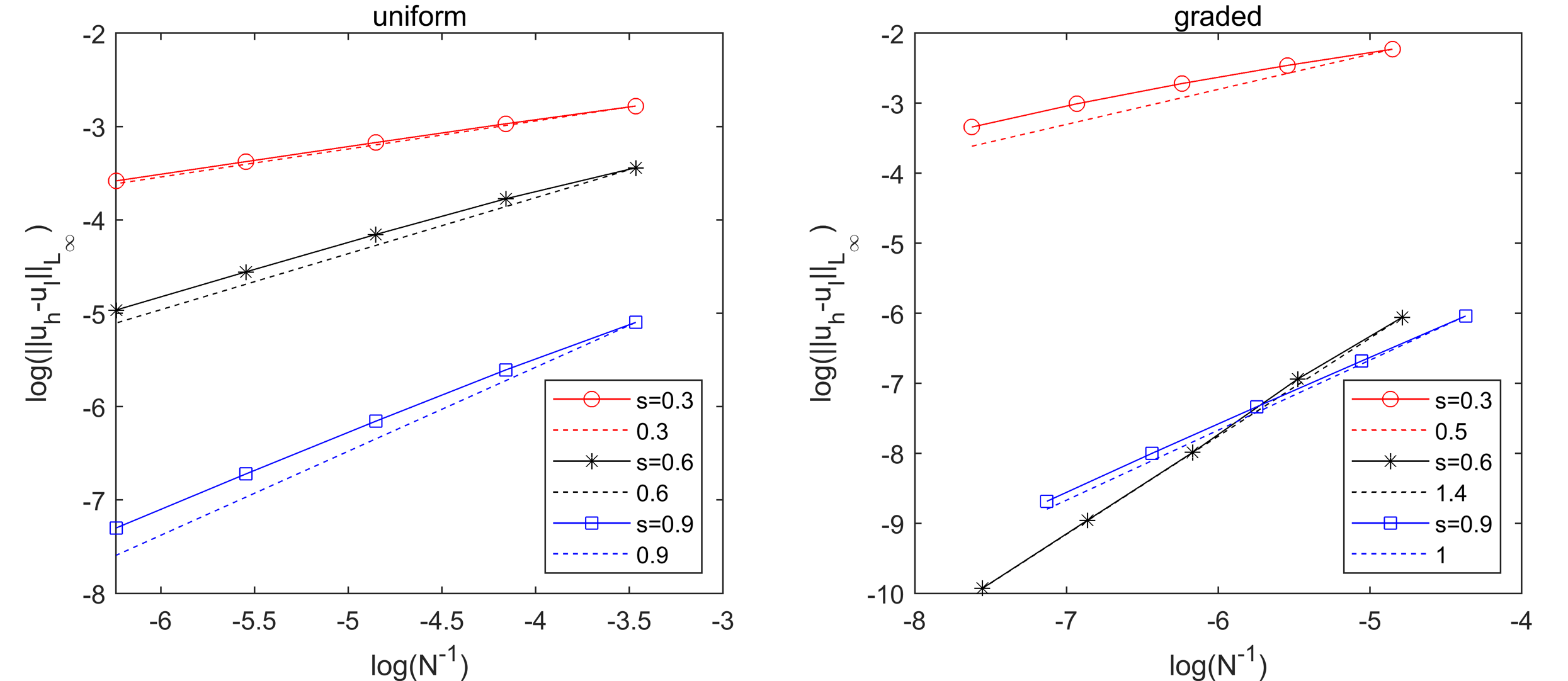
Figure 1 illustrates the convergence rates for both uniform and graded grids. According to [14, Section 7.1], the optimal choice for the pointwise estimate of the linear fractional Laplacian is , which will also be used in this test. The convergence rate over uniform grids is observed to be approximately , which is consistent with the behavior observed in the quasi-uniform grids for the linear case. Moreover, the graded grid yields a significantly improved convergence rate. It is worth noting that for the linear case, the convergence order under the optimal choice is , which is also observed for some cases (e.g., ). However, for other cases, the strategy of choosing in (14) based on the local distance to the contact set may lead to different convergence rates compared to those analyzed for the linear case.
5.2. Quantitative behavior and comparison of different policy iterations
In this section, Problem (1) is investigated over the domain . The force is set as , and the obstacle function is given by
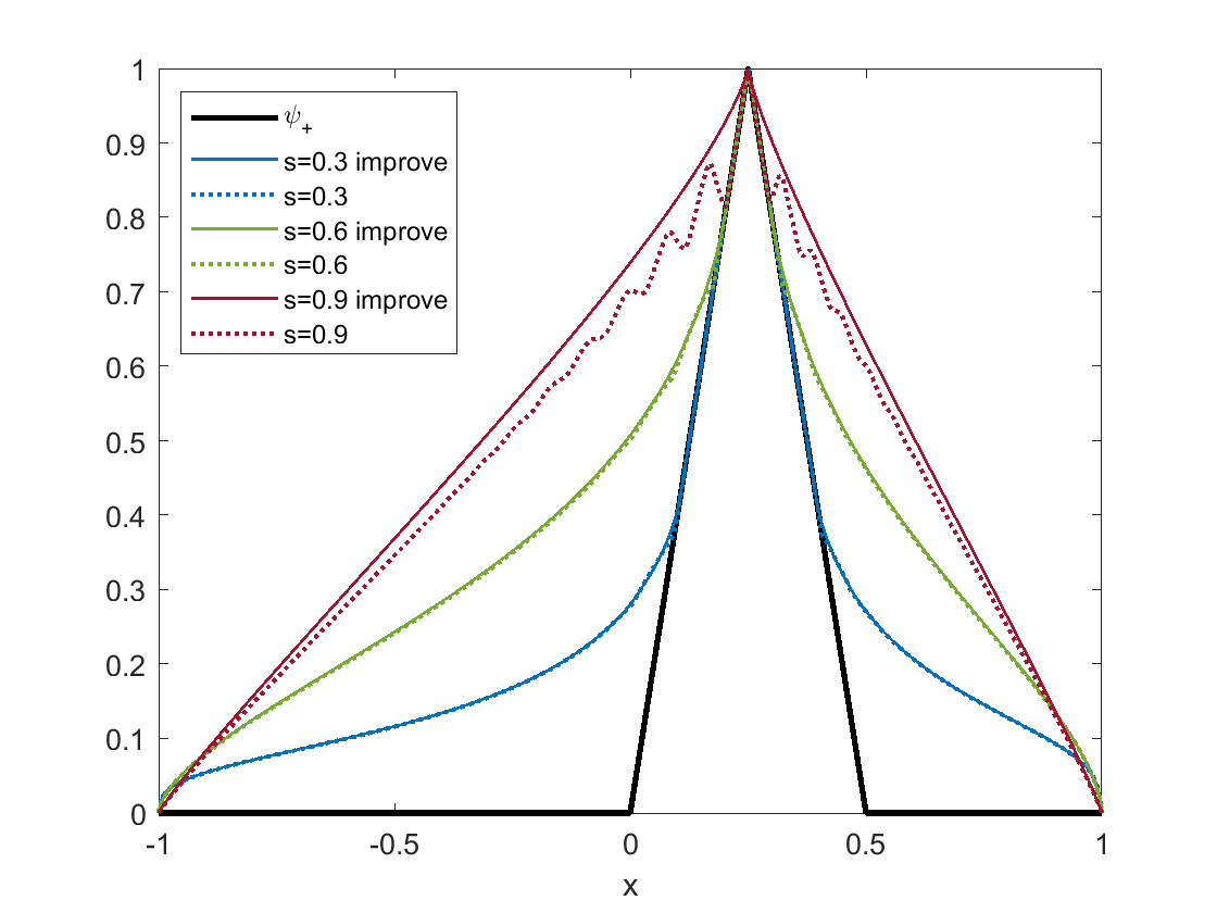
In Figure 2, the numerical solutions obtained for different values of are presented below. A clear qualitative difference is observed between the solutions for different choices of . When , the discrete solution resembles the expected solution of the classical obstacle problem, where the operator is effectively replaced by . As decreases, the solution approaches . Throughout the experiments, a consistent observation is made that as increases, the contact set decreases and always contains the point .
The difference between the improved method and the original method is remarkable. Observations reveal that when using the original method with larger values of , oscillations occur near the free boundary due to the handling of the singular part across it.On the other hand, the improved method yields a numerically smoother solution without oscillations. As decreases, the solutions obtained by the two methods become closer to each other, and the differences diminish.
5.3. Convergence history of improved policy iteration
Next, the convergence history of the improved policy iteration (Algorithm 2) is examined. The experiment is conducted with , and the obstacle function is defined as follows:
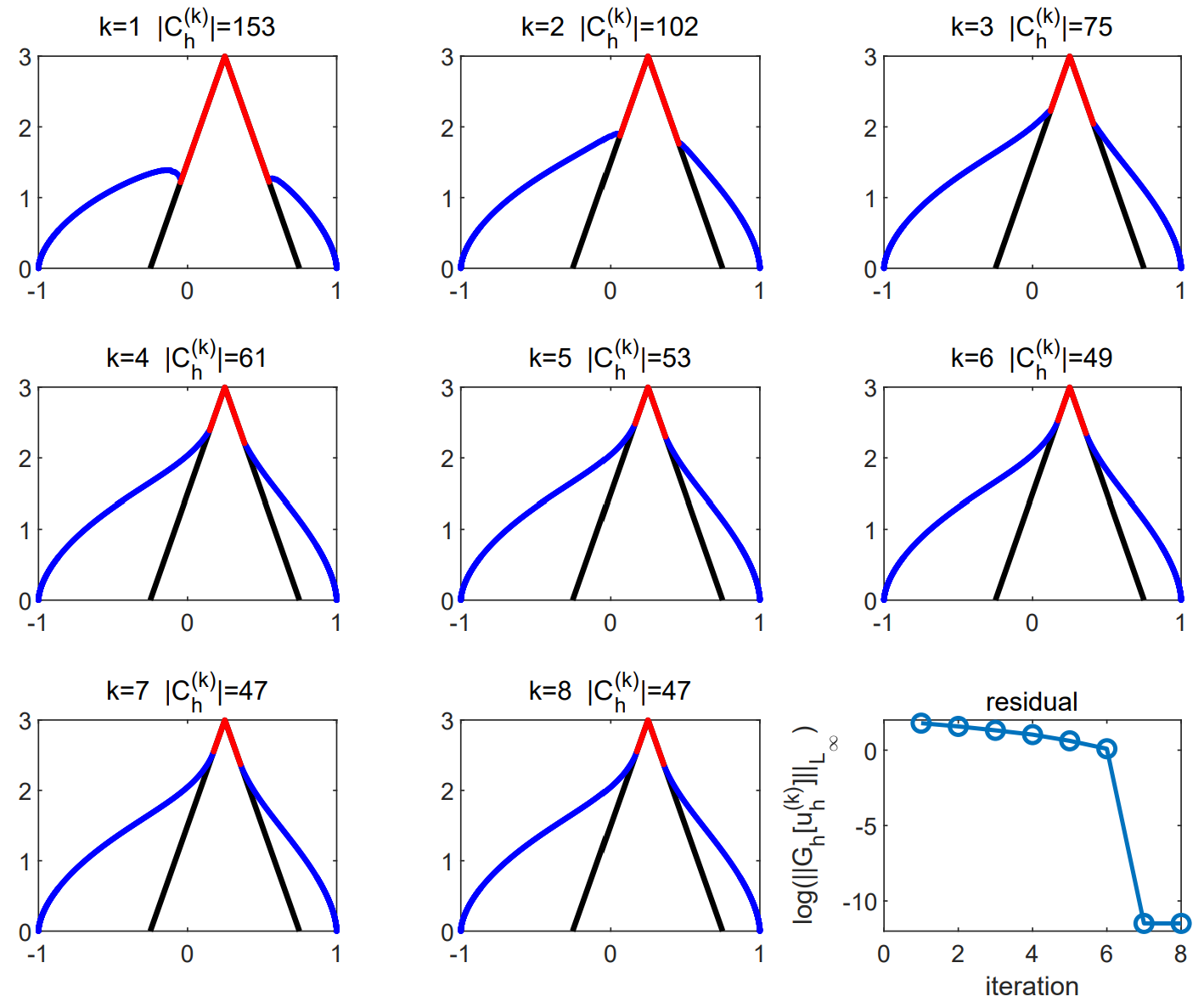
As mentioned in Remark 4.3, it is highly likely that the improved algorithm possesses the property of an increasing solution sequence (or decreasing discrete contact set) as stated in Theorem 4.1 for the standard algorithm. In this experiment, as demonstrated in Figure 3, the convergence profile is observed through the values of .
| 126 | 254 | 510 | 1022 | 118 | 237 | 476 | 953 | 77 | 155 | 311 | 623 | |
| iterations | 4 | 5 | 5 | 6 | 5 | 6 | 7 | 8 | 6 | 7 | 9 | 11 |
Furthermore, the actual number of iterations obtained in the experiments is presented in Table 1. It can be observed that the actual number of iterations required is significantly smaller than the theoretical upper bound . Additionally, as the grid is refined, the algorithm’s performance remains stable. This demonstrates the efficiency of our algorithm.
5.4. 2D test
Finally, problem (1) is considered in the domain with , and the obstacle function is given by
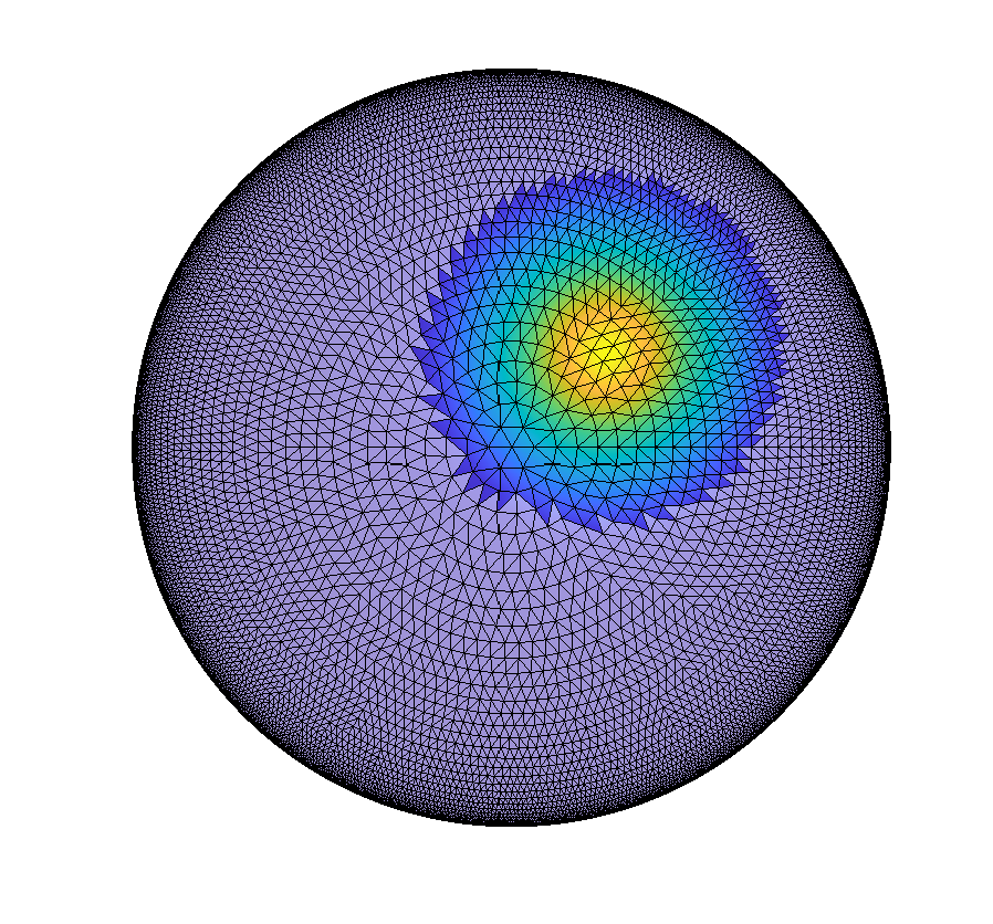
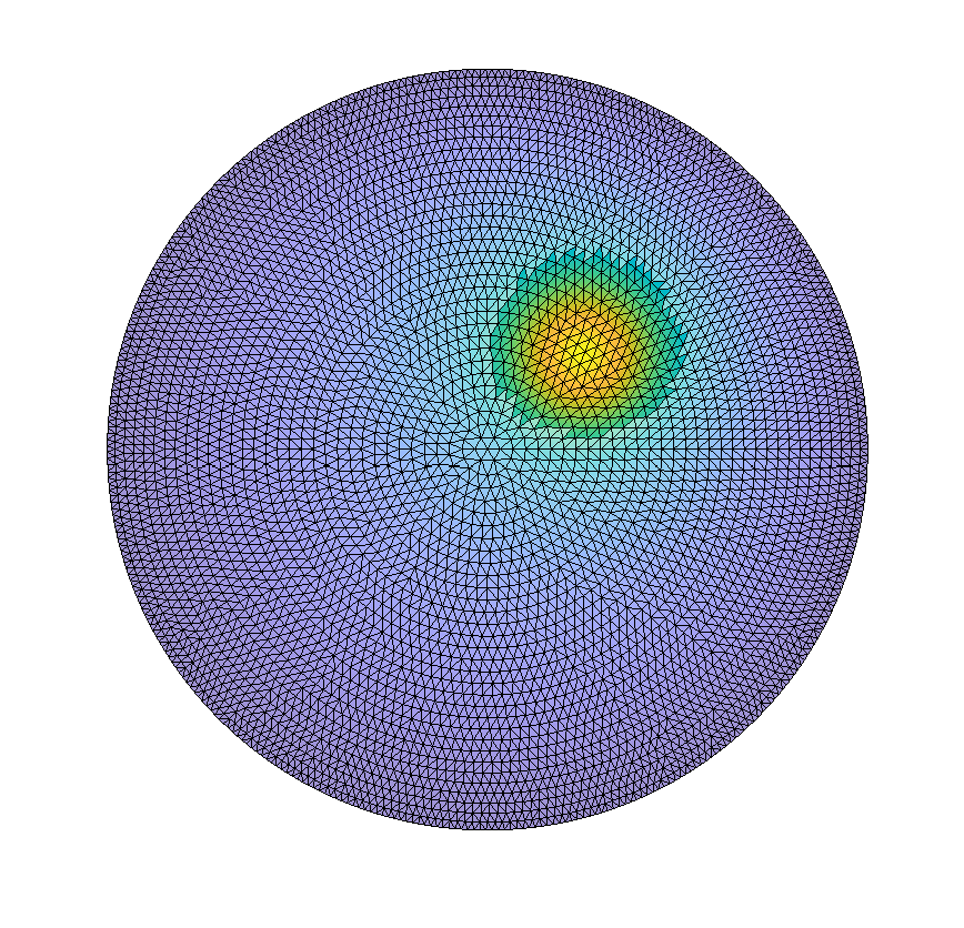
For , the numerical solution requires 13,395 degrees of freedom, and the number of improved policy iterations is 4. Conversely, for , the numerical solution involves 4,253 degrees of freedom, and the number of improved policy iterations is 10. The number of iterations increases as grows, but significantly less than , as also observed in the 1D case. As expected, the 2D numerical results demonstrate similar qualitative characteristics as observed in 1D.
6. Conclusion
In this paper, a discrete scheme for the fractional obstacle problem is proposed, which is based on the monotone discretization for the fractional Laplace operator. Utilizing the distinctive structure of the problem (10) and conducting a comprehensive study of the discrete operator, the study reveals that the nonlinear discrete operator upholds the discrete comparison principle. Based on this property, the existence, uniqueness, and uniform boundedness of numerical solutions are established.
Due to the limited regularity of the true solution near the domain boundary, a graded grid has been introduced to capture this behavior. For solving nonlinear problems, the policy iteration method is used. Benefiting from the monotonicity of the discrete scheme of the fractional Laplace operator, the policy iterative process can converge in finite iterations. Moreover, considering the reduced regularity of the actual solution near the contact set boundary, the discretization of the fractional Laplacian has been adaptively refined by iteratively updating contact nodes. This refinement has led to an improved policy iteration approach. In contrast to the conventional policy iteration, this improved method demonstrates superior numerical performance across a range of numerical experiments. One-dimensional and two-dimensional examples are provided to support the theoretical results.
Appendix A proof of Proposition 2.3 under a weak assumption of
Proposition 2.3 is proven, assuming . The proof follows closely the global Hölder estimate for the linear problem [20], so only the main thread will be sketched. First, some elementary tools are recalled.
Proposition A.1 (Corollary 2.5 in [20]).
Assume that is a solution of in . Then for every ,
where the constant depends only on and .
Lemma A.2 ( estimate of obstacle problem, [16]).
For and , the solution of (1) satisfies with the following bounds:
The proof of Lemma A.2 follows from the comparison principle. As a direct consequence, the estimate of the fractional Laplace equation implies the following inequality for and :
Lemma A.3 (supersolution, Lemma 2.6 in [20]).
There exist and a radial continuous function satisfying
By the Lemma A.2 and Lemma A.3, one could construct an upper barrier for by scaling and translating the supersolution. The proof of Lemma A.4 is similar to the Lemma 2.7 in [20]. The only difference is for each point , when constructing the upper barrier on the ball touched from outside, the radius of the ball not only depends on the exterior ball condition of , but also depends on which appeared in the assumption (4) for the contact set.
Lemma A.4 (-boundary behavior).
Let be a bounded satisfying the exterior ball condition and let , u is the solution of (1). Then
where is a constant depending only on , and . Here, .
The following Hölder seminorm estimate is provided by the above Lemma, which plays a vital role in the proof of Proposition 2.3.
Proposition A.5 (improved interior Hölder estimate).
Let satisfies the exterior ball condition, , u is the solution of (1), then and for all wa have the following seminorm estimate in
where and the constant depending only on , and .
Proof. Using the standard mollifier technique, it can be assumed that is smooth. Note that Let . The equation for is given by:
| (17) |
Furthermore, by employing the inequality in (see Lemma A.4), the following result can be deduced:
| (18) |
Further, (18) and Lemma A.4 also imply that
whence
| (19) |
References
- [1] Gabriel Acosta and Juan Pablo Borthagaray. A fractional laplace equation: regularity of solutions and finite element approximations. SIAM Journal on Numerical Analysis, 55(2):472–495, 2017.
- [2] Guy Barles and Panagiotis E Souganidis. Convergence of approximation schemes for fully nonlinear second order equations. Asymptotic analysis, 4(3):271–283, 1991.
- [3] Olivier Bokanowski, Stefania Maroso, and Hasnaa Zidani. Some convergence results for howard’s algorithm. SIAM Journal on Numerical Analysis, 47(4):3001–3026, 2009.
- [4] Juan Pablo Borthagaray, Ricardo H Nochetto, and Abner J Salgado. Weighted sobolev regularity and rate of approximation of the obstacle problem for the integral fractional laplacian. Mathematical Models and Methods in Applied Sciences, 29(14):2679–2717, 2019.
- [5] JH Bramble and BE Hubbard. On the formulation of finite difference analogues of the dirichlet problem for poisson’s equation. Numerische Mathematik, 4(1):313–327, 1962.
- [6] Susanne C Brenner and Ridgwat Scott. The mathematical theory of finite element methods. Springer New York, NY, 2008.
- [7] Luis Caffarelli and Luis Silvestre. An extension problem related to the fractional laplacian. Communications in partial differential equations, 32(8):1245–1260, 2007.
- [8] Luis A Caffarelli, Sandro Salsa, and Luis Silvestre. Regularity estimates for the solution and the free boundary of the obstacle problem for the fractional laplacian. Inventiones mathematicae, 171:425–461, 2008.
- [9] Jose A Carrillo, Matias G Delgadino, and Antoine Mellet. Regularity of local minimizers of the interaction energy via obstacle problems. Communications in Mathematical Physics, 343:747–781, 2016.
- [10] Siwei Duo, Hans Werner van Wyk, and Yanzhi Zhang. A novel and accurate finite difference method for the fractional laplacian and the fractional poisson problem. Journal of Computational Physics, 355:233–252, 2018.
- [11] Siwei Duo and Yanzhi Zhang. Accurate numerical methods for two and three dimensional integral fractional laplacian with applications. Computer Methods in Applied Mechanics and Engineering, 355:639–662, 2019.
- [12] Xiaobing Feng and Max Jensen. Convergent semi-lagrangian methods for the monge-ampère equation on unstructured grids. SIAM Journal on Numerical Analysis, 55(2):691–712, 2017.
- [13] Xavier Fernández-Real. The thin obstacle problem: a survey. Publicacions Matemàtiques, 66(1):3–55, 2022.
- [14] Rubing Han and Shuonan Wu. A monotone discretization for integral fractional laplacian on bounded lipschitz domains: Pointwise error estimates under hölder regularity. SIAM Journal on Numerical Analysis, 60(6):3052–3077, 2022.
- [15] Yanghong Huang and Adam Oberman. Numerical methods for the fractional laplacian: A finite difference-quadrature approach. SIAM Journal on Numerical Analysis, 52(6):3056–3084, 2014.
- [16] Roberta Musina, Alexander I Nazarov, and Konijeti Sreenadh. Variational inequalities for the fractional laplacian. Potential Analysis, 46:485–498, 2017.
- [17] R Nochetto, Dimitrios Ntogkas, and Wujun Zhang. Two-scale method for the monge-ampère equation: Convergence to the viscosity solution. Mathematics of Computation, 88(316):637–664, 2019.
- [18] Xavier Ros-Oton. Nonlocal elliptic equations in bounded domains: a survey. Publicacions matematiques, pages 3–26, 2016.
- [19] Xavier Ros-Oton. Obstacle problems and free boundaries: an overview. SeMA Journal, 75(3):399–419, 2018.
- [20] Xavier Ros-Oton and Joaquim Serra. The dirichlet problem for the fractional laplacian: regularity up to the boundary. Journal de Mathématiques Pures et Appliquées, 101(3):275–302, 2014.
- [21] Manuel S Santos and John Rust. Convergence properties of policy iteration. SIAM Journal on Control and Optimization, 42(6):2094–2115, 2004.
- [22] Sylvia Serfaty. Systems of points with coulomb interactions. European Mathematical Society Magazine, (110):16–21, 2018.
- [23] Antonio Signorini. Sopra alcune questioni di elastostatica. Atti della Societa Italiana per il Progresso delle Scienze, 21(2):143–148, 1933.
- [24] Luis Silvestre. Regularity of the obstacle problem for a fractional power of the laplace operator. Communications on Pure and Applied Mathematics, 60(1):67–112, 2007.
- [25] Peter Tankov. Financial modelling with jump processes. CRC press, 2003.
- [26] Hendrik Jan van Linde. High-order finite-difference methods for poisson’s equation. Mathematics of Computation, 28(126):369–391, 1974.
- [27] Jinchao Xu and Ludmil Zikatanov. A monotone finite element scheme for convection-diffusion equations. Mathematics of Computation, 68(228):1429–1446, 1999.