Brownian yet non-Gaussian thermal machines

Abstract

We investigate the performance of a Brownian thermal machine working in a heterogeneous heat bath. The mobility of the heat bath fluctuates and it is modelled as an Ornstein–Uhlenbeck process. We trap the Brownian particle with time-dependent harmonic potential and by changing the stiffness coefficient and bath temperatures, we perform a Stirling cycle. We numerically calculate the average absorbed work, the average ejected heat and the performance of the heat pump. For shorter cycle times, we find that the performance of a Brownian yet non-Gaussian heat pump is significantly higher than the normal (Gaussian) heat pump. We numerically find the coefficient of performance at maximum heating power.

Introduction.—The development of heat engines led to the industrial revolution. Two centuries ago, in 1824, Sadi Carnot showed that the maximum efficiency of a heat engine depends only on the temperatures of the hot ($T_{h}$) and cold ($T_{c}$) reservoirs. The Carnot efficiency is given by $\eta_{C}=1-T_{c}/T_{h}$ carn . To achieve this maximum efficiency, the heat engine needs to operate reversibly, which takes an infinite amount of time. Therefore, the power output becomes zero by definition, which makes no practical use. Finite power output is crucial for any practical application. Efficiency at maximum power (EMP) is another fundamental parameter to studying real heat engines. Novikov for atomic power plants, Curzon and Ahlborn for endo-reversible heat engines showed that the efficiency at maximum power is $\eta_{NCA}=1-\sqrt{T_{c}/T_{h}}$ nov125 ; cur22 . EMP for heat engines has been actively investigated in the last four decades and208 ; and157 ; rub127 ; sal211 ; dev570 ; sal354 ; van190 ; esp150 ; joh052 ; tu312 ; ben230 ; izu100 ; bra070 ; her037 ; ang746 ; izu180 ; wan062 ; iyy500 ; rya050 ; pro220 ; iyy012 ; joh0121 ; joh044 .

Apart from macroscopic heat engines, micrometre-sized heat engines have unique features where the fluctuations become significant bus43 . Ken Sekimoto identified the thermodynamic quantities, such as heat, work and internal energy for a Brownian particle at a single trajectory level sek123 . Now the framework is called stochastic thermodynamics seki ; sei126 . Schmiedl and Seifert modelled a stochastic Carnot heat engine and showed that the EMP is $\eta_{SS}=\eta_{C}/(2-\alpha\eta_{C})$ sch200 . Here $\alpha$ represents the dissipation due to a finite-time process. Several studies have been conducted on Brownian heat engines hol050 ; ran042 ; tu052 ; pro041 ; arg052 ; hol120 ; sch068 ; nak012 ; gom643 ; miu042 ; ye043 ; miu034 ; che024 ; lin022 . Using advanced experimental techniques, various microscopic heat engines have been realized in the lab bli143 ; qui588 ; mar67 ; kri113 . In particular, active heat engines attracted a lot of attention zak193 ; wul050 ; mar600 ; pie041 ; sah094 ; hol043 ; eke010 ; kum032 ; lee032 ; hol060 ; sza042 ; gro052 ; lee024 ; spe012 .

Recently, Wang et. al discovered a new class of diffusion process in which they found the normal diffusion of Brownian particle ($\langle x^{2}(t)\rangle\propto t$) with the Laplace displacement distribution (for a shorter time) wan151 ; wan481

$$\rho(x,t)\backsimeq\mbox{exp}\left(-\frac{|x|}{\lambda(t)}\right).$$ (1)

Here, the characteristic decay length $\lambda(t)$ varies as $\sqrt{t}$. Many physical and biological systems exhibit normal diffusion with the non-Gaussian displacement distribution hap111 ; lep198 ; ska256 ; gua333 ; mat042 ; cha022 . This Brownian yet non-Gaussian behaviour has been well studied by the concept of super-statistics wan481 ; hap111 and the diffusing diffusivity model chu098 ; che021 . In the diffusing diffusivity model, the diffusion coefficient is treated as a random variable and it is given by the square of the Ornstein–Uhlenbeck process che021 . In this work, we perform a Stirling cycle for a Brownian particle diffusing with fluctuating mobility. Our results show that the Brownian yet Non-Gaussian thermal machine works as a heat pump and performs significantly better than the usual Brownian heat pump for a shorter cycle time (see Fig. (4)).

Stochastic thermodynamics.—In this work, we only consider an overdamped regime. We use the following definitions to calculate the average thermodynamic quantities. The average internal energy is given by sch200

$$U\equiv\int V(x,\lambda(t))p(x,t)dx.$$ (2)

The average work done by the particle is defined as seki

$$W=\int_{t_{i}}^{t_{f}}dt\int\frac{\partial V(x,\lambda(t))}{\partial\lambda}\dot{\lambda}p(x,t)dx.$$ (3)

Here, $V(x,\lambda(t))$ is the external potential and $\lambda(t)$ is the time-dependent control parameter. $p(x,t)$ is the probability distribution of $x$ at time $t$. The justification for calling Eq. (3) as work can be found in Refs. sek123 and jar329 . Using the thermodynamic first law like energy balance, we can calculate the absorbed heat from the thermal bath as ran042

$$Q=W-\Delta U,$$ (4)

where $\Delta U$ is the change in internal energy during the isothermal process.

The Model.—When Brownian particles diffuse in the heterogeneous medium it encounters varying mobility with time. It can be due to the dynamic evolution of the medium or the different regions with different mobilities hap111 ; lep198 ; ska256 ; gua333 ; mat042 ; cha022 ; kha064 . Chechkin et. al used the set of Langevin equations to explain the diffusion of Brownian particle in an environment with fluctuating mobility che021 . Here, we consider the Brownian particle trapped by the time-dependent harmonic potential

$$V(x,\lambda(t))=\frac{\lambda(t)}{2}x^{2},$$ (5)

where $\lambda(t)$ is the externally controllable stiffness coefficient. The Langevin equation of motion for a Brownian particle diffusing in a heterogeneous medium is governed by the following set of equations

$$\frac{dx}{dt}=-\mu(t)\lambda(t)x+\sqrt{2\mu(t)\kappa_{B}T}\;\xi(t),$$ (6)

$$\mu(t)=\chi^{2}(t),$$ (7)

$$\frac{d\chi(t)}{dt}=-\frac{\chi(t)}{\tau^{\prime}}+\sigma\zeta(t).$$ (8)

Here, $x(t)$ is the position of the Brownian particle at time $t$. We restrict our studies to one dimension. $\mu(t)$ is the fluctuating mobility che021 . $\kappa_{B}$ is the Boltzmann constant and $T$ is the bath temperature. $\xi(t)$ is the Gaussian white thermal noise with $\langle\xi(t)\rangle=0$, $\langle\xi(t)\xi(t^{\prime})\rangle=\delta(t-t^{\prime})$. The fluctuating mobility is defined as a square of the random variable $\chi$ to make sure it is positive che021 . The random variable $\chi(t)$ is given by Ornstein–Uhlenbeck process (Eq. (8)) and its explanation can be found che021 . $\tau^{\prime}$ is the correlation time of the Ornstein–Uhlenbeck process. $\zeta(t)$ is white Gaussian noise with $\langle\zeta(t)\rangle=0$, $\langle\zeta(t)\zeta(t^{\prime})\rangle=\delta(t-t^{\prime})$ che021 . $\sigma$ is the strength of the fluctuating noise $\zeta(t)$. For simplicity, we consider the single random variable $\chi(t)$. In general, $\chi(t)$ can have $n$ degrees of freedom che021 . The distribution of the random variable $\chi(t)$ at time $t$ is denoted by $f(\chi,t)$ and it evolves according to the Fokker-Planck equation risk

$$\frac{\partial f(\chi,t)}{\partial t}=-\frac{\partial}{\partial\chi}\left[-\frac{\chi}{\tau^{\prime}}-\frac{\sigma^{2}}{2}\frac{\partial}{\partial\chi}\right]f(\chi,t).$$ (9)

For a stationary state, the distribution of $\chi$ becomes

$$f(\chi)=\frac{1}{\sqrt{\pi\sigma^{2}\tau^{\prime}}}\mbox{exp}\left(-\frac{\chi^{2}}{\sigma^{2}\tau^{\prime}}\right).$$ (10)

We use the Euler-Muryama numerical method to integrate the stochastic differential equations (6)-(8). We set the initial values $x(0)=0$ and $\chi(0)$ has been chosen randomly from the distribution given in Eq. (10).

Now, we apply the framework of stochastic thermodynamics to the fluctuating mobility system and construct a thermodynamic cycle to study its energetics. Experimentally realizing the Carnot cycle for Brownian particles is very difficult since it contains adiabatic processes. However, Martínez et. al accomplished microscopic adiabatic process for an underdamped Brownian particle by precisely controlling the phase space volume mar120 . The microscopic adiabatic process for a non-Gaussian system is not yet realized. Therefore, we study the Stirling cycle, which consists of two isothermal processes at different temperatures and two isochoric processes which connecting them. The schematic diagram of stochastic Stirling cycle is given in Fig. 1.

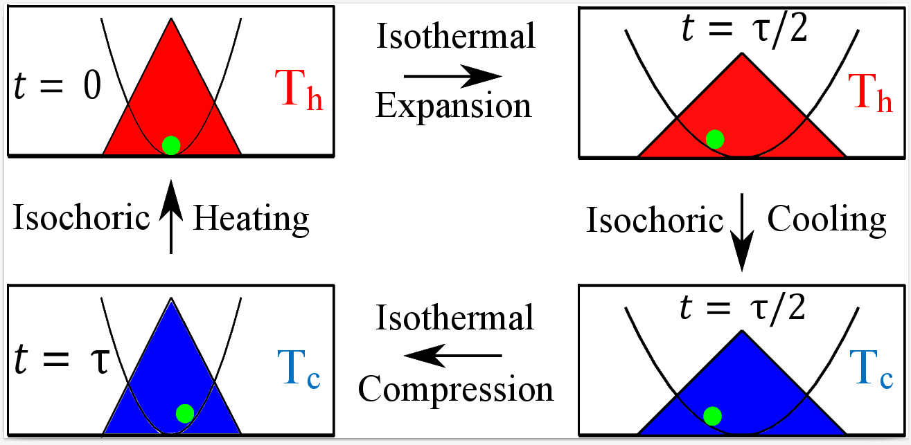
Figure 1: The schematic diagram of the Stirling cycle for a Brownian particle diffusing with fluctuating mobility. The solid parabolic curve represents the harmonic potential. The shaded red (blue) region represents the probability distribution of displacement when a Brownian particle in a hot (cold) bath at temperature $T_{h}$ ($T_{c}$). The probability distribution plotted on a logarithmic scale. $\tau$ is the cycle time. It has to be mentioned that the position of a Brownian particle after a cycle time $\tau$ is random.

Isothermal expansion process.— The Brownian particle is kept in a hot reservoir at temperature $T_{h}$ with the initial stiffness coefficient $\lambda_{h}$. We linearly decrease the stiffness coefficient to its lower value $\lambda_{l}$ for the period $t=0$ to $t=\tau/2$, which is easily realizable in experiments bli143 . This is equivalent to the volume expansion of the macroscopic heat engine. We use the following protocol gom643

$$\lambda_{1}(t)=\lambda_{h}-\frac{2}{\tau}\Delta\lambda t.$$ (11)

Here, $\Delta\lambda\equiv\lambda_{h}-\lambda_{l}$. The work done by the particle is

$$w_{1}=-\frac{\Delta\lambda}{\tau}\int_{0}^{\frac{\tau}{2}}x^{2}(t)dt.$$ (12)

Isochoric Cooling.—Keeping the stiffness coefficient constant, we decrease the temperature of the bath from $T_{h}$ to $T_{c}$ instantaneously. Therefore, the probability distribution of displacement does not change. However, in experiments, it takes a few milliseconds to cool the bath temperature from $T_{h}$ to $T_{c}$ bli143 , which can be neglected as compared with the cycle time. The work done by the particle during an isochoric process is zero since there is no change in the external control parameter bli143 .

Isothermal compression process.—Now, keeping the bath temperature at $T_{c}$. The stiffness coefficient is increased linearly for the period $t=\tau/2$ to $t=\tau$ as the protocol is given below gom643

$$\lambda_{3}(t)=\lambda_{l}-\Delta\lambda\left(1-\frac{2}{\tau}t\right).$$ (13)

The work done on the particle is calculated as

$$w_{3}=\frac{\Delta\lambda}{\tau}\int_{\frac{\tau}{2}}^{\tau}x^{2}(t)dt.$$ (14)

Isochoric Heating.—Finally, the bath temperature increased from $T_{c}$ to $T_{h}$, instantaneously, while keeping the stiffness coefficient constant. Nevertheless, in Blickle and Bechinger experiment, the isochoric heating process is achieved in less than one millisecond bli143 . Again, the isochoric heating process does not contribute to the work since there is no change in external control parameters. Using Eq. (4), we can calculate the heat transferred during the isothermal expansion process as

$$q_{h}=-\frac{\Delta\lambda}{\tau}\int_{0}^{\frac{\tau}{2}}x^{2}(t)dt-\frac{1}{2}\left[\lambda_{l}x\left(\frac{\tau}{2}\right)^{2}-\lambda_{h}x(0)^{2}\right].$$ (15)

Similarly, the heat transferred during the isothermal compression process becomes

$$q_{c}=\frac{\Delta\lambda}{\tau}\int_{\frac{\tau}{2}}^{\tau}x^{2}(t)dt-\frac{1}{2}\left[\lambda_{h}x(\tau)^{2}-\lambda_{l}x\left(\frac{\tau}{2}\right)^{2}\right].$$ (16)

The total work consumed by the Brownian particle is calculated by using the energy conservation law. Therefore, the consumed work becomes $w=q_{h}+q_{c}+\Delta u$, which is random in nature. $\Delta u$ becomes zero only on average. The ensemble average of total consumed work is given by $W=Q_{h}+Q_{c}$ ran042 .

Numerical Simulation.—When we perform a Stirling cycle for an ensemble of Brownian particles. The final position of Brownian particles ($x(\tau)$) is a random variable. To get the performance of stochastic heat devices independent of $x(\tau)$, first, we need to run many cycles until the mean-squared displacement of $x(m\tau)$ and $x((m+1)\tau)$ becomes equal, where $m$ is the number of cycles performed. Then the probability distribution satisfies the following condition, $p_{ss}(x,t)=p_{ss}(x,t+\tau)$, which is called the time-periodic steady state (TPSS) ran042 ; gom643 ; kum032 . If the ensemble of Brownian particles once reaches a TPSS, then it will no longer have the memory of its initial position $x(0)=0\,\mu m$(micrometer). Brownian particle in a homogeneous medium reaches a steady state after a few cycles. However, our system takes a huge number of cycles to reach a steady state which is not feasible. Therefore, we keep track of the cumulative of square displacement updated after each cycle for an ensemble of particles. We subtract the mean-square displacement averaged over cycles and an ensemble of particles from the cumulative mean square displacement. The average of this quantity is precision which from the Central limit theorem becomes smaller with more number of cycles. The precision decides when the particles have reached a steady state and the thermodynamic quantities have reached the desired accuracy. Therefore, we start to calculate the thermodynamic quantities for a Stirling cycle. In our calculations, we consider the ensembles of $10^{5}$ particle trajectories to compute the average quantities. For integration, we use the step size $dt=10^{-5}s$. We set the following parameters. The high and low values of stiffness coefficients, respectively as $\lambda_{h}=5pN/\mu m$ (pN-pico Newton), and $\lambda_{l}=1pN/\mu m$. The above $\lambda$’s are easily accessible in the lab gom643 . Temperatures of the hot and cold reservoirs, respectively as $T_{h}=363.15$K, and $T_{c}=278.15$K. The amplitude of fluctuation of $\chi$ is $\sigma=1\>\mu m^{1/2}pN^{-1/2}s^{-1}$ and the relaxation time $\tau^{\prime}=1s$. The Boltzmann constant $\kappa_{B}=1.38\times 10^{-5}pN\mu mK^{-1}$. To compare our results with the constant mobility case, we consider the following Langevin equation

$$\frac{dx}{dt}=-\mu\lambda(t)x+\sqrt{2\mu\kappa_{B}T}\;\xi(t),$$ (17)

where $\mu$ is the mobility. $\xi(t)$ is the Gaussian white noise with $\langle\xi(t)\rangle=0$, $\langle\xi(t)\xi(t^{\prime})\rangle=\delta(t-t^{\prime})$. We set $\mu=26.5258\>\mu mpN^{-1}s^{-1}$.

Results and Discussion.—Next, we present our numerical results. The figures are plotted in a semi-logarithmic manner where the x-axis is scaled logarithmically. In Fig. (2), we plot the input heat, absorbed work and ejected heat as a function of cycle time $\tau$. The heat absorbed from the cold bath $Q_{c}$ increases monotonically with time and the ejected heat to the hot bath $Q_{h}$ decreases monotonically with time. However, the absorbed work initially increases with cycle time $\tau$ and attains its maximum and then starts to decrease.

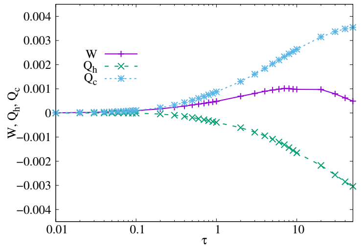
Figure 2: The average absorbed heat, consumed work, and ejected heat are plotted as functions of cycle time $\tau$. Here, the cycle time $\tau$ is plotted on a logarithmic scale.

In Fig. (3), we plot heating power ($Q_{h}/\tau$) as a function of cycle time $\tau$. The solid line represents the heating power of a Brownian yet non-Gaussian heat pump (BNGHP) and the dashed curve represents the Gaussian heat pump (GHP). In the case of BNGHP, initially, the heating power increases with time and reaches its maximum value around $\tau=0.04s$. Further, it decreases and attains its second minimum. Again the heating power increases with $\tau$. However, the heating power of GHP increases with the cycle time monotonically.

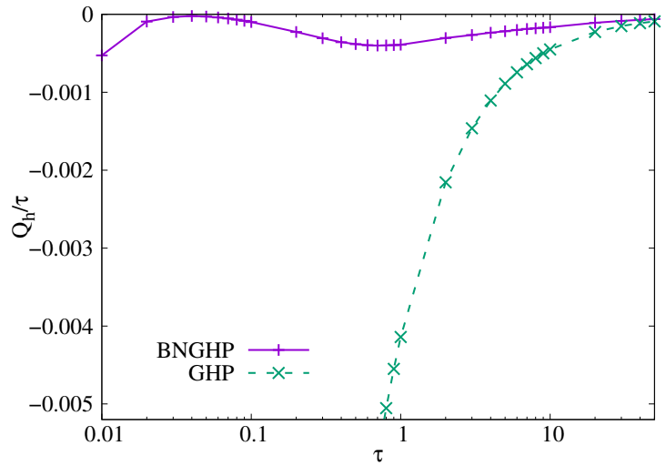
Figure 3: The heating power for Brownian yet non-Gaussian heat pump and Brownian heat pump are plotted as a function of cycle time $\tau$. Here, the cycle time $\tau$ varies on a logarithmic scale.

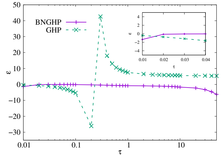
Figure 4: The performance of the Brownian yet non-Gaussian heat pump and Brownian heat pump are plotted as a function of cycle time $\tau$. The solid line represents the COP of the Brownian yet non-Gaussian heat pump. The dashed curve represents the COP of the Brownian heat pump. Inset shows the magnified view of the coefficient of performance for initial cycle times. It has to be noted that the cycle time $\tau$ in the figure and inset are plotted on the logarithmic scale.

The average coefficient of performance of a stochastic heat pump is given by

$$\epsilon=\frac{Q_{h}}{W}.$$ (18)

In Fig. (4), we plot the coefficient of performance as a function of cycle time $\tau$. Our results show that for cycle time $\tau=0.01s$ the COP of GHP is higher than the COP of BNGHP. For the range $0.02s<\tau\leq 0.2s$, the COP of BNGHP is significantly higher than the COP of GHP. That is for a cycle time less than the mobility correlation time $\tau^{\prime}$, the change in the mobility is negligible, and an ensemble of particles are diffusing with different mobility which mimics a spatially heterogeneous environment (see Eqs. (7) and (8), the initial value of mobility is randomly chosen from Eq. (10)) for further discussion see Ref. che021 . From Figs. (3) and (4), we find that for a BNGHP, the COP at maximum cooling rate is $0.0230587$.

Conclusion.—In this work, we studied the performance of a Brownian yet non-Gaussian thermal machine which works as a heat pump, where the inhomogeneity of the thermal bath is considered. We used the Euler-Muryama numerical method to calculate the average thermodynamic quantities such as the absorbed heat, absorbed work and ejected heat. Our results showed that the Brownian yet non-Gaussian heat pump performs significantly better as compared with the normal (Gaussian) heat pump for a shorter cycle time (see Fig. 4)). Further, we find that, for a BNGHP the heating power becomes maximum when the cycle time is around $\tau=0.04s$. We numerically evaluated the coefficient of performance at maximum heating power as $\epsilon=0.0230587$.

Future outlook.—The Brownian yet non-Gaussian heat pump can be easily realized in the lab. Chakraborty and Roichman artificially created spatial heterogeneity by using micropillars cha022 . With optical tweezers, one can create a harmonic potential to trap the Brownian particle. By varying the laser intensity and bath temperatures, the Stirling cycle can be easily accomplished bli143 . Entangled F-actin networks can also be used to realize BNGHP wan151 . Some active systems show varying diffusion coefficients due to the time evolution of the medium or the heterogeneity present in the environment. It will be interesting to study the energetics of diffusing diffusivity models for active systems kha064 . Further, in our future study, we would like to investigate the Brownian yet non-Gaussian heat devices with the external fluctuating force, which can increase the effective temperature of the Brownian particle mar032 . We are also interested in extending the present work in the quantum domain.

S.G. acknowledges the support from Interdisciplinary Cyber Physical Systems (ICPS) program of the Department of Science and Technology (DST), India, Grant No. DST/ICPS/QuEST/Theme-1/2019/13. J.E.T. thanks Ralf Metzler for useful discussion.

I.I. is delighted to dedicate this article to S. V. M. Satyanarayana who has been teaching free physics classes on Sundays to research aspirants for over a quarter century. I am one of the beneficiaries of his Sunday class.

I. I. and J. E. T. equally contributed to this work.

References

- (1) S. Carnot, Réflexions sur la Puissance Motrice du Feu, et sur les Machines Propres á Développer cette Puissance (1824).
- (2) I. Novikov, J. Nucl. Energy 7, 125 (1958).
- (3) F. L. Curzon, and B. Ahlborn, Am. J. Phys. 43, 22 (1975).
- (4) B. Andresen, R. S. Berry, A. Nitzan, and P. Salamon, Phys. Rev. A 15, 2086 (1977).
- (5) B. Andresen, P. Salamon, and R. S. Berry, J. Chem. Phys. 66, 1571 (1977).
- (6) M. H. Rubin, Phy. Rev. A 19, 1272 (1979).
- (7) P. Salamon, A. Nitzan, B. Andresen, and R. S. Berry, Phys. Rev. A 21, 2115 (1980).
- (8) A. De Vos, Am. J. Phys. 53, 570 (1985).
- (9) P. Salamon, and A. Nitzan, J. Chem. Phys. 74, 3546 (1981).
- (10) C. Van den Broeck, Phys. Rev. Lett. 95, 190602 (2005).
- (11) M. Esposito, R. Kawai, K. Lindenberg, and C. Van den Broeck, Phys. Rev. Lett. 105, 150603 (2010).
- (12) R. S. Johal, Phys. Rev. E 100, 052101 (2019).
- (13) Z. C. Tu, J. Phys. A 41, 312003 (2008).
- (14) G. Benenti, K. Saito, and G. Casati, Phys. Rev. Lett. 106, 230602 (2011).
- (15) Y. Izumida, and K. Okuda, Europhys. Lett. 97, 10004 (2012).
- (16) K. Brandner, K. Saito, and U. Seifert, Phys. Rev. Lett. 110, 070603 (2013).
- (17) A. C. Hernández, A. Medina, J. M. M. Roco, J. A. White, and S. Velasco, Phys. Rev. E 63, 037102 (2001).
- (18) F. Angulo-Brown, J. Appl. Phys. 69, 7465 (1991).
- (19) Y. Izumida, and K. Okuda, Phys. Rev. Lett. 112, 180603 (2014).
- (20) Y. Wang, Phys. Rev. E 90, 062140 (2014).
- (21) I. Iyyappan, and R. S. Johal, Europhys. Lett. 128, 50004 (2019).
- (22) A. Ryabov, and V. Holubec, Phys. Rev. E 93, 050101(R) (2016).
- (23) K. Proesmans, B. Cleuren, and C. Van den Broeck, Phys. Rev. Lett. 116, 220601 (2016).
- (24) I. Iyyappan, and M. Ponmurugan, Phys. Rev. E 97, 012141 (2018).
- (25) R. S. Johal, Phys. Rev. E 96, 012151 (2017).
- (26) R. S. Johal, and R. Rai, Phys. Rev. E 105, 044145 (2022).
- (27) C. Bustamante, J. Liphardt and F. Ritort, Phys. Today 58, 43 (2005).
- (28) K. Sekimoto, J. Phys. Soc. Jpn. 66, 1234 (1997).
- (29) K. Sekimoto, Stochastic Energetics, Lecture Notes in Physics Vol. 799 (Springer, New York, 2010).
- (30) U. Seifert, Rep. Prog. Phys. 75, 126001 (2012).
- (31) T. Schmiedl and U. Seifert, Europhys. Lett. 81, 20003 (2008).
- (32) V. Holubec, J. Stat. Mech.: Theory Exp. P05022 (2014).
- (33) S. Rana, P. S. Pal, A. Saha, and A. M. Jayannavar, Phys. Rev. E 90, 042146 (2014).
- (34) Z. C. Tu, Phys. Rev. E 89, 052148 (2014).
- (35) K. Proesmans, Y. Dreher, M. Gavrilov, J. Bechhoefer, and C. Van den Broeck, Phys. Rev. X 6, 041010 (2016).
- (36) A. Argun, J. Soni, L. Dabelow, S. Bo, G. Pesce, R. Eichhorn, and G. Volpe, Phys. Rev. E 96, 052106 (2017).
- (37) V. Holubec, A. Ryabov, Phys. Rev. Lett. 121, 120601 (2018).
- (38) F. Schmidt, A. Magazzú, A. Callegari, L. Biancofiore, F. Cichos, and G. Volpe, Phys. Rev. Lett. 120, 068004 (2018).
- (39) K. Nakamura, J. Matrasulov, and Y. Izumida, Phys. Rev. E 102, 012129 (2020).
- (40) J. R. Gomez-Solano, Front. Phys. 9, 643333 (2021).
- (41) K. Miura, Y. Izumida, and K. Okuda, Phys. Rev. E 103, 042125 (2021).
- (42) Z. Ye, F. Cerisola, P. Abiuso, J. Anders, M. Perarnau-Llobet, and V. Holubec, Phys. Rev. Res. 4, 043130 (2022).
- (43) K. Miura, Y. Izumida, and K. Okuda, Phys. Rev. E 105, 034102 (2022).
- (44) Y. H. Chen, J. -F. Chen, Z. Fei, and H. T. Quan, Phys. Rev. E 106, 024105 (2022).
- (45) W. Lin, Y. -H. Liao, P. -Y. Lai, and Y. Jun, Phys. Rev. E 106, L022106 (2022).
- (46) V. Blickle, and C. Bechinger, Nat. Phys. 8, 143 (2012).
- (47) P. A. Quinto-Su, Nat. Commun. 5, 5889 (2014).
- (48) I. A. Martínez, É. Roldán, L. Dinis, D. Petrov, J. M. R. Parrondo, and R. A. Rica, Nat. Phys. 12, 67 (2016).
- (49) S. Krishnamurthy, S. Ghosh, D. Chatterji, R. Ganapathy, and A. K. Sood, Nat. Phys. 12, 1134 (2016).
- (50) R. Zakine, A. Solon, T. Gingrich, and F. Van Wijland, Entropy 19, 193 (2017).
- (51) R. Wulfert, M. Oechsle, T. Speck, and U. Seifert, Phys. Rev. E 95, 050103(R) (2017).
- (52) D. Martin, C. Nardini, M. E. Cates, and É. Fodor, Europhys. Lett. 121, 60005 (2018).
- (53) P. Pietzonka, É. Fodor, C. Lohrmann, M. E. Cates, and U. Seifert, Phys. Rev. X 9, 041032 (2019).
- (54) A. Saha, and R. Marathe, J. Stat. Mech.: Theory Exp. 094012 (2019).
- (55) V. Holubec, S. Steffenoni, G. Falasco, and K. Kroy, Phys. Rev. Res. 2, 043262 (2020).
- (56) T. Ekeh, M. E. Cates, and É. Fodor, Phys. Rev. E 102, 010101 (2020).
- (57) A. Kumari, P. S. Pal, A. Saha, and S. Lahiri, Phys. Rev. E 101, 032109 (2020).
- (58) J. S. Lee, J. -M. Park, and H. Park, Phys. Rev. E 102, 032116 (2020).
- (59) V. Holubec, and R. Marathe, Phys. Rev. E 102, 060101(R) (2020).
- (60) G. Szamel, Phys. Rev. E 102, 042605 (2020).
- (61) G. Gronchi, and A. Puglisi, Phys. Rev. E 103, 052134 (2021).
- (62) J. S. Lee, and H. Park, Phys. Rev. E 105, 024130 (2022).
- (63) T. Speck, Phys. Rev. E 105, L012601 (2022).
- (64) B. Wang, S. M. Anthony, S. C. Bae, and S. Granick, Proc. Natl. Acad. Sci. U.S.A. 106, 15160 (2009).
- (65) B. Wang, J. Kuo, S. C. Bae, and S. Granick, Nat. Mater. 11, 481 (2012).
- (66) S. Hapca, J. W. Crawford, and I. M. Young, J. R. Soc. Interface 6, 111 (2009).
- (67) K. C. Leptos, J. S. Guasto, J. P. Gollub, A. I. Pesci, and R. E. Goldstein, Phys. Rev. Lett. 103, 198103 (2009).
- (68) M. J. Skaug, J. Mabry, and D. K. Schwartz, Phys. Rev. Lett. 110, 256101 (2013).
- (69) J. Guan, B. Wang, and S. Granick, ACS Nano 8, 3331 (2014).
- (70) M. Matse, M. V. Chubynsky, and J. Bechhoefer, Phys. Rev. E 96, 042604 (2017).
- (71) I. Chakraborty, and Y. Roichman, Phys. Rev. Res. 2, 022020(R) (2020).
- (72) M. V. Chubynsky, and G. W. Slater, Phys. Rev. Lett. 113, 098302 (2014).
- (73) A. V. Chechkin, F. Seno, R. Metzler, and I. M. Sokolov, Phys. Rev. X 7, 021002 (2017).
- (74) C. Jarzynski, Annu. Rev. Condens. Matter Phys. 2, 329 (2011).
- (75) S. M. J. Khadem, N. H. Siboni, and S. H. L. Klapp, Phys. Rev. E 104, 064615 (2021).
- (76) H. Risken, The Fokker–Planck Equation: Methods of Solution and Applications, 2nd ed (Springer, Berlin, 1989).
- (77) I. A. Martínez, É. Roldán, L. Dinis, D. Petrov, and R. A. Rica, Phys. Rev. Lett. 114, 120601 (2015).
- (78) I. A. Martínez, É. Roldán, J. M. R. Parrondo, and D. Petrov, Phys. Rev. E 87, 032159 (2013).