Advancing Ad Auction Realism:
Practical Insights & Modeling Implications

Abstract

This paper proposes a learning model of online ad auctions that allows for the following four key realistic characteristics of contemporary online auctions: (1) ad slots can have different values and click-through rates depending on users’ search queries, (2) the number and identity of competing advertisers are unobserved and change with each auction, (3) advertisers only receive partial, aggregated feedback, and (4) payment rules are only partially specified. We model advertisers as agents governed by an adversarial bandit algorithm, independent of auction mechanism intricacies. Our objective is to simulate the behavior of advertisers for counterfactual analysis, prediction, and inference purposes. Our findings reveal that, in such richer environments, “soft floors” can enhance key performance metrics even when bidders are drawn from the same population. We further demonstrate how to infer advertiser value distributions from observed bids, thereby affirming the practical efficacy of our approach even in a more realistic auction setting.

1 Introduction

Online ad auctions are an integral part of contemporary e-commerce. As end users interact with services or online stores such as Google, Facebook, or Amazon, advertisers compete to secure slots, aiming to display their ads to those prospective customers who are most likely to engage with them, and eventually lead to conversions.

The prevalence of such auctions has led to the development of a large literature in both Economics and Computer Science. The vast majority of these contributions focus on relatively simple auction formats, in which one or more ad slots are sold using so-called generalized first- or second-price auctions (Edelman et al., 2007; Varian, 2009). These mechanism adapt the first- and second-price mechanisms from “textbook” auction theory (Myerson, 1981; Krishna, 2009) to account for the fact that online advertising services often charge prices per click rather than per impression.

However, real-world online ad auction are highly complex. This makes it virtually impossible to analyze equilibrium bidding behavior and compare the performance (e.g., revenues) of different auction formats. As a result, businesses selling online ad space lack principled guidance as to which auction format to adopt.

We propose that simulating advertisers’ behavior using well-understood online-learning algorithms can provide such guidance. To demonstrate this, we develop an approach that allows for the following key departure from standard auction formats and their generalized variants:

1. The value of an impression or click for a given ad (and slot), as well as its click through rate, may vary depending on the shopper’s query, identity, and history. Advertisers can choose “targeting clauses” to only bid on certain sets of queries, but cannot condition their bid on individual queries.

2. The number and identity of advertisers changes from one auction to the next. However, advertisers do not observe who they are facing in each individual auction.

3. Advertisers receive only incomplete feedback about the outcome of each individual auction. In particular, they do not observe other advertisers’ bids, and they only learn the market-clearing price if they win the auction.

4. Pricing mechanisms are often incompletely specified. For instance, ad services may indicate that reserve prices are used, but not what they are, or how they are computed.

To reflect the scant information bidders possess when they participate in real-world ad auctions, we choose learning algorithms that only require feedback about individual rewards, and are not tailored to any specific auction format. In addition, we want our model to be able to handle auctions in which the number of participants and bid space is realistic. We focus on two algorithms: Hedge (Auer et al., 1995) and EXP3-IX (Lattimore and Szepesvári, 2020, Chap. 12). These algorithms, with known regret bounds, are applied in auction learning literature and exemplify full- and partial-information algorithms respectively.

We provide two sets of results. In the first set presented in §4.1 and §4.2, we assign artificial valuations to bidders and simulate their bidding behavior. We consider both small and large number of bidders. We also allow a dense bid grid, especially compared with earlier studies, and complex auction environments with multi-query targeting and soft-floor reserve prices. These results demonstrate how our approach enables performance comparisons across different auction formats. In symmetric, single-query environments, our approach reassuringly approximates theoretical predictions, including revenue equivalence (Myerson, 1981), indicating that despite differing bidding behaviors across auction formats, the seller’s revenues remain roughly constant. On the other hand, we find that, with multi-query targeting, soft floors can lift revenues, even if bidders are ex-ante symmetric. The second set of results presented in §4.3, instead demonstrates how to use our approach to solve the inverse problem, inferring bidders’ valuations through an iterative parameter search matching bid data. To do so, we employ aggregate bid data from an actual production environment (a major e-commerce website).

1.1 Related Literature

There is a vast literature in Economics that studies games from the perspective of learning agents; Fudenberg and Levine (1998) provides an authoritative account.

In computer science, the literature on online learning in auctions can be roughly divided into two branches. The first takes the perspective of the seller and studies the design of revenue-maximizing auctions; recent studies include Roughgarden and Wang (2019), Guo et al. (2021), and Jeunen et al. (2023). This branch of the literature studies sellers who employ learning algorithms, but bidders are not explicitly modelled.

The second branch instead takes the perspective of a single bidder who uses learning algorithms to guide her bidding process. Weed et al. (2016) focus on second-price auctions for a single good, and assume that the valuation can vary either stochastically or adversarially in each auction. In a similar environment, Balseiro et al. (2018) and Han et al. (2020) study contextual learning in first-price auctions, where the context is provided by the bidder’s value. For auctions in which the bidder must learn her own value (as is often the case in the settings we consider), Feng et al. (2018) proposes an improved version of the EXP3 algorithm that attains a tighter regret bound. There is also a considerable literature that studies optimal bidding with a budget constraint using reinforcement-learning: e.g., Wu et al. (2018), Ghosh et al. (2020), and references therein.

Our paper differs from the above references since it models the interaction among bidders who adopt online learning algorithms. In this sense, it is closer in spirit to the Economics literature on learning in games. In addition, unlike the present paper, the cited references assume that the winning bidder observes her valuations and payment in each period; some of these papers leverage insights that depend on specific auction format; and all are concerned with auctions for a single object or ad slot.

To the best of our knowledge, the closest papers to our own are Kanmaz and Surer (2020), Elzayn et al. (2022), and Jeunen et al. (2022). The first reports on experiments using a multi-agent reinforcement-learning model in simple sequential (English) auctions for a single object, with a restricted bid space. Our analysis focuses on simultaneous bidding in scenarios that are representative of actual online ad auctions. The second focuses on position (multi-slot) auctions and, among other results, reports on experiments using no-regret learning (specifically, the Hedge algorithm we also use) under standard generalized second-price and Vickerey-Groves-Clarke pricing rules. Our analysis is complementary in that we allow for different targeting clauses and more complex pricing rules such as “soft floors”. The third describes a simulation environment similar to ours that is mainly intended to help train sophisticated bidding algorithms for advertisers. We differ in that we allow for bids broadly targeting multiple queries, and focus on learning algorithms that allow us to model auctions with a large number of bidders; in addition, we demonstrate how to infer values from observed bids.

Feng et al. (2021) establish the convergence to equilibrium of learning algorithms in first- and second-price auctions, as well as multi-slot VCG mechanisms. Our results in §4.1 provide an empirical counterpart to their theoretical results, but also add nuance as to the speed of convergence of different algorithms in realistic-sized auctions. Hartline et al. (2015) establish the convergence of no-regret learning to coarse Bayes correlated equilibrium in general games with incomplete information; we leverage their results in §3.2.

Nekipelov et al. (2015) proposes techniques for estimating agents’ valuations in generalized second-price auctions, which stands in contrast to our method that directly utilizes agents’ learning algorithms and is independent of the specific auction format. In a different direction, Rahme et al. (2021) study revenue maximization in auctions as a mechanism design problem, assuming a static “no regret” constraint for bidders, which in general differs from the no regret condition in online learning. Peysakhovich et al. (2019) presents a method to predict player behavior in an unseen game. Unlike our approach, they base their predictions on an $\epsilon$-Bayesian Nash equilibrium instead of no-regret learning. Bichler et al. (2021) suggests a method to calculate $\epsilon$-Bayesian Nash equilibria in sealed-bid auctions, focusing more on approximating equilibria, as opposed to directly modeling bidder learning behavior.

Finally, we mention equilibrium analyses of bidding and ad exchanges that provide results related to our simulation findings. Choi and Sayedi (2019) analyze auctions in which a new entrant’s click-through rate is not known to the publisher. Despotakis et al. (2021) demonstrates that, with competing ad exchanges, a multi-layered auction involving symmetric bidders can result in a scenario where first-price auctions, and soft floors in general, yield higher revenue than second-price auctions. When multiple slots are offered, Rafieian and Yoganarasimhan (2021) shows that, when advertisers can target their bids to specific placements in second-price auctions, total surplus increases, but the effect on publisher revenues is ambiguous, the key difference being that we consider a single slot with randomly arriving queries, rather than multiple slots that are always offered for sale.

2 Auction Model

This section introduces the auction model we analyze. For any finite set $\mathcal{X}$, we denote by $\Delta(\mathcal{X})$ the set of probability distributions on $\mathcal{X}$.

We fix a single ad slot, or position, within the ad service’s or publisher’s web page. Time is discrete and indexed by $t=1,2,\ldots,T$. In each time period $t$, a user visits the web page and submits a query, represented by a point $q$ in a finite set $Q$. The probability that query $q$ is submitted at time $t$ is given by the probability distribution $F_{Q}\in\Delta(Q)$. The ad service then runs an auction to determine which ad to show in the given slot.

There are $N$ (potential) bidders, whom we also refer to as advertisers, indexed by $i=1,\ldots,N$. Each bidder $i$ is characterized by a type $\tau_{i}$ drawn at the beginning of each period from a finite set $\mathcal{T}_{i}$ according to a distribution $F_{i}\in\Delta(\mathcal{T}_{i})$. We also fix functions $V_{i}:\mathcal{T}_{i}\times Q\to\mathbb{R}$ and $\mathit{CTR}_{i}:\mathcal{T}_{i}\times Q\to[0,1]$ such that, whenever bidder $i$’s type is $\tau_{i}\in\mathcal{T}_{i}$ and the shopper query is $q\in Q$, $i$’s value per click is $V_{i}(\tau_{i},q)$ and the ad click-through rate is $\mathit{CTR}_{i}(\tau_{i},q)$; these functions are in practice represented by matrices.

In every period, each bidder $i$ simultaneously submits a bid $b_{i}\in\mathbb{R}$ and a targeting clause $c_{i}\subset Q$; the interpretation is that the bidder intends to participate in the auction only if the user’s query is an element of $c_{i}$. The timing is as follows: first, bidder $i$ observes her type $\tau_{i}$; then, she places a bid $b_{i}$ and a targeting clause $c_{i}$; finally, the user query $q\in Q$ is realized. Thus, bidders cannot tailor their bid to the specific user query in a given period. On the other hand, their bids can and will in practice depend upon their realized type. The winner of the auction is the bidder with the highest score, i.e., the product of their bid and their click-through rate, provided they targeted the realized query. Formally, if the realized user query is $q$ and each bidder $i$ has type $\tau_{i}$, bids $b_{i}$, and targets $c_{i}$, then bidder $i$’s score is $s_{i}=b_{i}\cdot\mathit{CTR}_{i}(\tau_{i},q)$ if $q\in c_{i}$ and $0$ otherwise; the winner is any $i\in\arg\max_{j\in N:q\in c_{j}}s_{j}$. Ties are broken randomly.

If the realized user query is $q$, bidder $i$ wins the auction, and the charged price per click is $p$, then the average reward (payoff) to bidder $i$ with type $\tau_{i}$ is $\mathit{CTR}_{i}(\tau_{i},q)\cdot\left[V_{i}(\tau_{i},q)-p\right]$. Finally, if bidder $i$’s targeting clause $c_{i}$ does not include the realized $q$, or if it does but $b_{i}$ is not the winning bid, her payoff is 0.

The price charged to the winner depends upon the auction rules; we consider different cases in §4, so we defer the specifics until then. Similarly, we specify what bidders observe at the end of each period in §3, as that is a function of the learning algorithm under consideration. However, we maintain throughout that bidders only observe their own reward, and not others’ rewards or bids.

The concept of “type”, as introduced by Harsanyi (1967), is key to model games with incomplete information: in every period, each bidder $i$ knows the distribution $F_{j}$ of her opponents $j$, but not their realized type. In one common interpretation, there is a population of potential bidders for every bidder role $i$, each with distinct value per click and click-through rate; in each period $t$, and for every bidder role $i$, a specific element of the corresponding population is drawn according to $F_{i}$. A symmetric environment is one where the set of bidder types and their distributions are identical; we use this in §4 for aggregate-level bidding behavior analysis. One alternative interpretation is that there is a single player (a firm) for every bidder role $i$; her type can represent the fact that the firm may be selling a range of goods, with per-period variations in values and click-through rates reflecting product-specific margins and conversion rates, perhaps due to cost variability, promotions, etc.

Types can also be used to model (indirectly) a random number of bidders. Suppose that, for each bidder (or for a subset of bidders), we define a type $\tau_{i}^{0}$ who has zero value and click-through rate for every query. Then, in our learning algorithms, this bidder type will eventually stop bidding. Hence, out of $N$ potential bidders, only a subset may be active, the ones whose types are different from $\tau_{i}^{0}$. We assume type distributions are independent across bidders, although this could be relaxed as our learning algorithms do not rely on independence.

Standard auctions are a special case of our model in which there is a single query: this can be captured by assuming that the set $Q$ of queries is a singleton, say $\{q^{*}\}$. Thus, a bidder’s type $\tau_{i}$ fully characterizes her value for the object, and one may as well take $V_{i}$ to be the identity: $V_{i}(\tau_{i},q^{*})=\tau_{i}$. Traditional “textbook” auctions do not consider click-through rates; this can be captured by assuming that each function $\mathit{CTR}_{i}(\cdot)$ is identically equal to 1. However, pay-per-click auctions are common in advertising, so we consider them “standard” as well.

Targeting clauses provide flexibility in ad auctions. For instance, queries about USB chargers can vary in specificity and suggest differing shopper expertise. This results in varied values and click-through rates for advertisers, causing them to target different query types. For example, a wide-range product advertiser might target “USB charger” and “USB type C charger”, while an Apple-specific advertiser might target “iPhone charger”.

3 Learning Models

The two main learning models we analyze are Hedge (also referred to as Exponential Weights or Multiplicative Weights) algorithm (Auer et al., 1995; Freund and Schapire, 1997) and EXP3-IX (Kocák et al., 2014). We fix a grid $B$ of possible bid values. To streamline notation, for each bidder $i$ and time period $t$, we let $a_{i,\tau_{i},t}$ denote the pair $(b_{i},c_{i})\in B\times 2^{Q}\equiv A$ of bid and targeting clause chosen by bidder $i$ of type $\tau_{i}$ in period $t$. Relative to standard expositions of these algorithms (Lattimore and Szepesvári, 2020, e.g.), we add incomplete information and incorporate the draw of different queries in each iteration.

Each bidder type learns from their own observations, not those of other types of the same bidder, to accommodate incomplete information. Learning is not conditioned on the unobserved realized query, reflecting the reality of online ad auctions.

3.1 Model Setup for Auction Environment

We use the notation in Table 1 to describe the auction environment and learning algorithms. Suppose each bidder $i$ bids $b_{i}$ on clause $c_{i}$, and prices per query are $p=(p_{q})$. Denote by $c_{iq}$ the indicator function that equals 1 if and only if $q\in c_{i}$. Then bidder $i$’s expected utility if she wins the auction for the (non-empty) set of queries $\mathcal{Q}\subseteq\{0,\ldots,Q-1\}$, given her value and CTR for each query $q\in\mathcal{Q}$ as $v_{iq}$ and $CTR_{i,q}$ respectively, is

$$EU_{i}(b_{i},c_{i},p)=\sum_{q\in\mathcal{Q}}F_{Q}(q)\cdot CTR_{iq}\cdot c_{iq}\cdot\left[v_{iq}-p_{q}\right],$$ (1)

where the expectation is due to the random arrival of queries ($F_{Q}(q)$) and clicks ($CTR_{iq}$). In case of ties, for simplicity of implementation, we just divide the winner’s surplus $v_{iq}-p_{q}$ by $N$, rather than (as we should) the number of tying bidders. Losing bidders get 0 expected utility. Since the EXP3-IX algorithm requires rewards in $[0,1]$, we define the normalized reward of bidder $i$ as

$$r_{i}=\frac{EU_{i}(b_{i},c_{i},p)-(0-b_{\max})}{(v_{\max}-0)-(0-b_{\max})}=\frac{EU_{i}(b_{i},c_{i},p)+b_{\max}}{v_{\max}+b_{\max}}.$$ (2)

Table 1: Notation for online ad auction

Object	Notation
Bidders	$i=0,\ldots,N-1$
Time horizon	$T$
Bids	$b_{i}\in B\equiv\{0,...,b_{\max}\}$
Queries	$q\in\{0,...,Q-1\}$
Clause	$c_{i}=(c_{iq})_{q=0}^{Q-1}\in\{0,1\}^{Q}$
Value per bidder per query	$v_{iq}\in\{0,...,v_{\max}\}$
CTR per bidder per query	$CTR_{iq}\in[0,1]$
Normalized reward per bidder	$r_{i}\in[0,1]$

This is because the EU of a bidder cannot exceed the maximum value of the slot for any query if she were to get it for free, i.e., $v_{\max}-0$; and it is always at least as large as getting a worthless slot and paying the maximum bid for it, i.e., $0-b_{\max}$.

In our auction setting, we apply the Hedge and EXP3-IX algorithms, described in the Appendix. Bidders independently use these to update their actions based on observed rewards. Hedge assumes bidders observe rewards for all possible actions, leading to faster learning but less realistic scenarios. EXP3-IX assumes observation of the chosen action’s reward, providing a slower but more realistic learning process. Although Hedge is more computationally efficient and less dispersed, a deeper investigation of these algorithms’ distributional characteristics is suggested. We chose EXP3-IX over EXP3 due to its tighter bounds on realized regret, despite EXP3’s good expected regret guarantees.

3.2 Convergence to Equilibrium

Since both Hedge and EXP3-IX ensure that each type will have vanishing regret in the limit as $T\to\infty$, Lemma 10 in Hartline et al. (2015) implies that the resulting dynamics will converge to a version of correlated equilibrium for games with incomplete information. We now formally define this equilibrium notion for the class of games we consider.

For every bidder $i$, let $\mathbf{s}_{i}:\mathcal{T}_{i}\to B\times\{0,1\}^{Q}$ be a strategy for bidder $i$: for each type $\tau_{i}\in\mathcal{T}_{i}$, a strategy specifies a bid and a targeting clause: $\mathbf{s}_{i}(\tau_{i})=(b_{i},c_{i})$. Let $\mathbf{S}_{i}$ be the set of all such strategies for $i$, and define the Cartesian product sets $\mathbf{S}=\prod_{i}\mathbf{S}_{i}$ and $\mathbf{S}_{-i}=\prod_{j\neq i}\mathbf{S}_{j}$ as usual. For $\mathbf{s}\in\mathbf{S}$ and $\tau\in\prod_{i}\mathcal{T}_{i}$, by convention $\mathbf{s}(\tau)=\left(\mathbf{s}_{i}(\tau_{i})\right)_{i\in N}$; similarly, $\mathbf{s}_{-i}(\tau_{-i})=\left(\mathbf{s}_{j}(\tau_{j})\right)_{j\neq i}$.

To describe the outcome of the auction, for every query $q$, let $\mathbf{p}_{q}:(B\times\{0,1\}^{Q})^{N}\to\mathbb{R}$ denote the pricing rule of the auction, which associates the price charged to the winner with any vector of bids and targeting clauses. Furthermore, for each $i=0,\ldots,N-1$ and $q\in Q$, let $\mathbf{w}_{iq}:(B\times\{0,1\}^{Q})^{N}\to[0,1]$ denote the probability that bidder $i$ wins the auction for query $q$ given the bids and clauses submitted by all players. We assume that, for every query $q$ and tuple $(b,c)\in(B\times\{0,1\}^{Q})^{N}$, $\sum_{i}\mathbf{w}_{iq}(b,c)=1$ and $\mathbf{w}_{iq}(b,c)>0$ only if $c_{iq}=1$; that is, in order to win the auction for a query, the bidder must have included it in her targeting clause.

We can then define the payoff of bidder $i$’s type $\tau_{i}$, given a tuple $(b,c)\in(B\times\{0,1\}^{Q})^{N}$ of bids and targeting clauses for every player, as

$$U_{i}(b,c;\tau_{i})=\sum_{q=0}^{Q-1}F_{Q}(q)\cdot CTR_{iq}(\tau_{i})\cdot\mathbf{w}_{iq}(b,c)\cdot\left[V_{iq}(\tau_{i})-\mathbf{p}_{q}(b,c)\right].$$

With these definitions, a probability distribution $\sigma\in\Delta(\mathbf{S})$ is a coarse Bayes Correlated Equilibrium (coarse BCE) if, for every $i=0,\ldots,N-1$, $(b_{i},c_{i})\in B\times\{0,1\}^{Q}$, and $\tau_{i}\in\mathcal{T}_{i}$,

$$\mathrm{E}_{\mathbf{s}\sim\sigma,\tau_{j}\sim F_{j}:j\neq i}U_{i}(\mathbf{s}(\tau);\tau_{i}))\geq\mathrm{E}_{\mathbf{s}\sim\sigma,\tau_{j}\sim F_{j}:j\neq i}U_{i}\left((b_{i},c_{i}),\mathbf{s}_{-i}(\tau_{-i});\tau_{i}\right).$$

That is, for each type $\tau_{i}$, there is no single action $(b_{i},c_{i})$ that improves upon her payoff if she conforms to the profile $\sigma$. This differs from the notion of a (non-coarse) Bayes Correlated Equilibrium (Bergemann and Morris, 2016) in that it does not rule out more sophisticated deviations, in which type $\tau_{i}$ chooses different actions $b_{i},c_{i}$ for each recommended action $\mathbf{s}_{i}(\tau_{i})$ in the support of the marginal of the equilibrium distribution $\sigma$ on $i$’s strategy space $\mathbf{S}_{i}$.

4 Empirical Results

4.1 Standard auctions

We first consider a standard, symmetric auction environment with a single query, so $Q=\{q^{*}\}$, and pay-per-impression pricing, so all CTRs are equal to 1. We consider both a small auction with $N=2$ bidders, and a more realistic one with $N=10$ bidders. Values are uniformly distributed on a grid $B$ in the interval $[0,1]$. Formally, given the grid $B$, for all $i$, we let $\mathcal{T}_{i}=B$, $V_{i}(b,q^{*})=b$, $\mathit{CTR}_{i}(b,q^{*})=1$, and $F_{i}(b)=\frac{1}{|B|}$ for all $b\in B$. Furthermore, we allow all bids $b_{i}$ on the grid $B$.

In a second-price auction, it is a dominant strategy for every bidder to bid their value. In a first-price auction, with $N$ bidders, a continuum of values (uniformly distributed on $[0,1]$) and bids, the unique symmetric Bayesian Nash equilibrium is for each bidder to bid a fraction $\frac{N-1}{N}$ of their value. Furthermore, Myerson’s revenue equivalence applies, so the expected revenue for the advertising service is the same under both formats, namely $\frac{N-1}{N+1}$. We want to compare these theoretical predictions with the output of our learning algorithms with a fine enough grid $B$, and a long enough horizon $T$.

We choose $B=\{\frac{i}{20}:i=0,\ldots,20\}$ and $T=1,000,000$ for EXP3-IX. We also choose the tuning parameters optimally, as described in Lattimore and Szepesvári (2020) (Theorem 12.1, Chapter 12). Table 2 displays revenues for the advertising service in first- and second-price auctions under EXP3-IX, averaged over the last $10\%$ of the learning period, i.e., $100,000$ iterations, and 5 different runs of the algorithm, as well as the standard deviation of revenues across different runs.

Table 2: Standard single-item auction, EXP3-IX

Auction format	Mean Revenue	Std. Dev.
First price, $N=2$	$0.3474$	$0.0205$
Second price, $N=2$	$0.3346$	$0.0016$
First price, $N=10$	$0.780$	$0.0095$
Second price, $N=10$	$0.7723$	$0.0171$

Table 3 reports the results for Hedge. We choose $T=400,000$ and $\eta=0.02$. We averaged over 5 different runs of the algorithm and over the last $40,000$ time periods.

Table 3: Standard single-item auction, Hedge.

Auction format	Mean Revenue	Std. Dev.
First price, $N=2$	$0.3201$	$0.0018$
Second price, $N=2$	$0.3256$	$0.0018$
First price, $N=10$	$0.8305$	$0.0011$
Second price, $N=10$	$0.8334$	$0.0008$

The key take-away is that expected revenues are close to the theoretical value $\frac{1}{3}$ for $N=2$ under both Hedge and Exp3-IX. With $N=10$, Hedge again approximates the theoretical value $0.\overline{81}$, while Exp3-IX is not as close. Revenues do not vary much across different runs. Even when $N=2$, EXP3-IX required a considerably larger number of periods to achieve similar results as Hedge.

4.2 Soft floors

Zeithammer (2019) shows that, in a symmetric auction for a single object, bid functions are monotonic. As a consequence, the revenue equivalence theorem (Myerson, 1981) applies, and introducing soft floors in second-price auctions do not affect either the final allocation or the advertising service’s revenues. He then demonstrates by way of examples that, with asymmetric bid distributions, revenues in a second-price auction with a soft floor can be either higher or lower than in a standard second-price auction. In this section, we show that, in a more realistic environment in which types are multi-dimensional and bidders can choose which queries to target, different auction formats can yield different revenues even when bidder types are drawn from the same distribution.

Given a soft floor equal to $s$, the price is determined as follows; we describe the case of equal click-through rates for simplicity. Let $b_{(1)}$ and $b_{(2)}$ be the first- and, respectively, second-highest bids. If $b_{(2)}\geq s$, then $p=b_{(2)}$, as in a standard second-price auction. If $b_{(1)}\geq s>b_{(2)}$, then $p=s$, as if $s$ was a standard reserve price (“hard floor”). Crucially, if $s>b_{(1)}$, then the high bidder still wins the auction (on the contrary, with a standard reserve price, the seller would keep the object) and $p=b_{(1)}$.

For completeness, we first consider the symmetric, single-query environment of §4.1 and simulate an auction with a soft floor equal to $s=0.5$. Consistently with Zeithammer (2019), we find that soft floors have virtually no impact on revenues.

Next, we consider a multi-query environment, which is beyond the scope of Zeithammer (2019). We assume $N=3$ bidders, all with the same set of possible types $\mathcal{T}_{1}=\mathcal{T}_{2}=\mathcal{T}_{3}=\{1,2,3\}$. There are two queries, so $Q=\{1,2\}$. Values and click-through rates for all bidders are as described in Table 4. Thus, for example, $V_{i}(2,1)=0.25$ and $\mathit{CTR}_{i}(1,2)=0.1$. Both queries are equally likely, and all types are also equally likely. To clarify, these parameters are artificial and purposely chosen to illustrate the point. We let $B=\{\frac{i}{20}\>:\>i=0,\ldots,20\}$ and $T=1,000,000$.

Table 4: Values and Click-Through Rates for all bidders

$\tau_{i}$	$V_{i}(\tau_{i},1)$	$\mathit{CTR}_{i}(\tau_{i},1)$	$V_{i}(\tau_{i},2)$	$\mathit{CTR}_{i}(\tau_{i},2)$
1	0.5	0.3	0.25	0.1
2	0.25	0.1	1	0.1
3	0.25	0.1	1	0.2

Table 5 reports expected revenues per impression (where expectations are taken over search queries, bidder types, and click-through rates) for EXP3-IX, averaged over 5 runs. Table 6 reproduces the results for Hedge, with $T=400,000$.

Table 5: Multi-query auctions and soft floors, EXP3-IX output for $T=1\mathrm{M}$, averaged over 5 runs.

Auction format	Mean Revenue	Std. Dev.
First price	$0.0830$	$0.0007$
Second price	$0.0509$	$0.0008$
Soft floor $s=0.65$	$0.0813$	$0.0007$

Table 6: Multi-query auctions and soft floors, Hedge output for $T=400\mathrm{K}$, averaged over 5 runs.

Auction format	Mean Revenue	Std. Dev.
First price	$0.0691$	$0.0016$
Second price	$0.0857$	$0.0001$
Soft floor $s=0.65$	$0.0741$	$0.0061$

Our first key finding is that, as anticipated, the three auction formats yield different expected revenues. Soft-floor reserve prices can impact revenues; thus, our simulations provide some support to this common industry practice. Under Hedge, revenues are higher in soft-floor reserve price auctions than in first-price auctions, but second-price auctions perform best. With EXP3-IX, second-price auctions do not fare as well; the highest revenues come from first-price auctions, with soft-floor pricing behind.

A second key finding is that EXP3-IX results do not align with Hedge even when run for longer periods. Each panel in Figure 1 shows the frequency of bids in the final $40,000$ periods of the learning algorithm, summed over 5 runs, divided by type and targeting clause (i.e., queries actually targeted). The main take-away point is that every type eventually learns to choose a specific targeting clause and for the most part also places fairly concentrated bids.

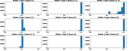
Figure 1: Bids in second-price auction under Hedge

Now compare with Figure 2, which summarizes predicted bids for bidder 1 under EXP3-IX, with Figure 1 above (again we sum over 5 runs and only look at the last $100,000$ periods).

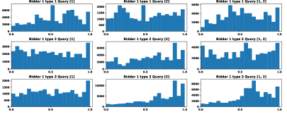
Figure 2: Bidder 1’s bids in second-price auction, EXP3-IX

Type 1 occasionally bids on one or both queries, showing little convergence even after one million runs. EXP3-IX requires more experimentation, as it only learns from played actions, while Hedge converges faster but assumes learning about unplayed actions. This supports the idea that leveraging knowledge of the pricing mechanism enhances performance. Hedge outperforms due to its reliance on full reward information. We suggest that incorporating heuristics into EXP3-IX may partially address this imbalance; we leave this to future work.

4.3 Inferring values and bid shading

Next, we use our approach to infer the distribution of bidders’ values from the observed distribution of bids. We utilize Hedge for this inference procedure, due to the bid dispersion observed with EXP3-IX (§4.2).

The analysis is based on aggregated bid data for two specific shopper queries in an e-commerce setting, one characterized by low traffic and the other by high traffic. The data aggregation process converts all bids into a bid per impression, so we set all click-through rates to 1. Thus, we apply our analysis to a symmetric environment with a single query, unit click-through rates, and two different scenarios, one with a low number of bidders (low traffic) and one with a high number of bidders (high traffic).

We normalize all bids to lie in a grid $B$ in the interval $[0,4]$. Specifically, we take $B=\{\frac{i}{10}:i=0,\ldots,40\}$. We then define the set of types to be quantiles of the given bid distribution, with a step size of $0.1$. We initialize the procedure by setting the inferred value distribution to the observed bid distribution. We then apply multiple iterations of the following procedure. First, we run the learning algorithm and derive a predicted bid distribution.

Then, we adjust inferred values for each quantile. To do so, we use the following heuristic. Suppose that, for a given quantile, the currently inferred value is $v$, the observed bid is $b^{o}$, and the predicted bid is $b^{p}$. This means that the predicted extent of bid shading (reducing one’s bid below one’s value) is $\sigma=\frac{b^{p}}{v}$. We then update $v$ according to $v\leftarrow v+\alpha\left(\frac{b^{o}}{\sigma}-v\right)$. Finally, since the inferred values are associated with increasing quantiles, we apply a “flattening” step to ensure that they are indeed increasing. This completes one inference iteration. Intuitively, a bidder with value $\frac{b^{o}}{\sigma}$ who bids by applying a shading factor of $\sigma$ will bid exactly $b^{o}$, the actually observed bid for this quantile. We then adjust the inferred $v$ in the direction of $\frac{b^{o}}{\sigma}$, applying a learning rate adjustment $\alpha=0.2$.

Figure (3) represents the inferred values of bidders for the low-traffic search query, under the three pricing rules we analyzed in §4.2: first price, second price, and soft floor with a reserve price of $\$0.65$. We chose these pricing rules arbitrarily, to demonstrate their impact on the inference process. We used 8 iterations of the inference procedure and 3 runs of the learning algorithm per iteration, each with $T=500,000$, averaging bids over the last $50,000$ periods.

As anticipated, we observe bid shading in the first price auction, as well as within the lower to middle quantiles in the case of the soft floor. The second price auction also displays bid shading at lower quantiles. We hypothesize that this deviation from theoretical prediction is due to a lack of learning amongst low-valuation types: players with low valuation win rarely, so the feedback they receive is coarse on most periods and hence insufficient to converge to bidding one’s value.

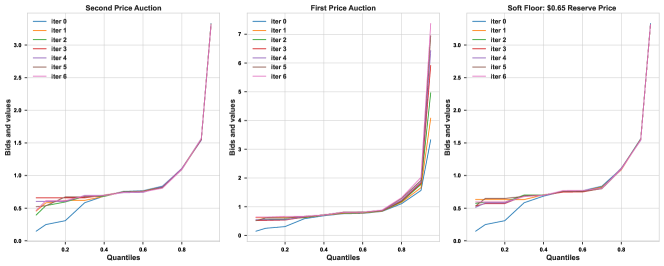
Figure 3: Value inference in three auction formats for the low traffic search query

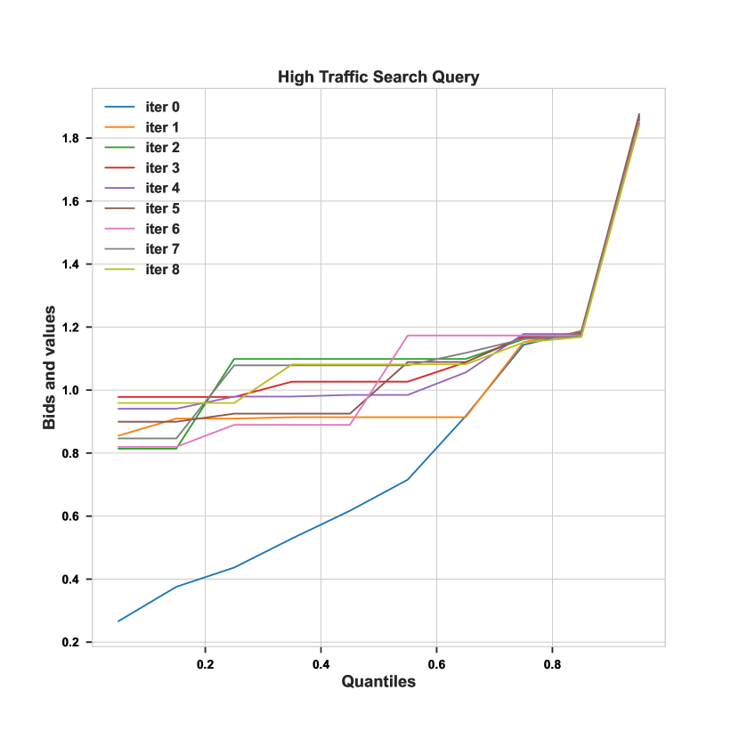
Figure 4: Inferring values for the high traffic search query. In this experiment, we set $T=800,000$ and applied $8$ inference iterations. The results show that inferred values converge in a few iterations even in a more realistic auction environment.

Figure 4 analyzes the high-traffic query. We increased the length of the simulation to $T=800,000$ periods. As one can see, even with a large number of bidders, inferred values converge in a few iterations.

5 Conclusions

Online learning algorithms can serve as effective tools in modeling bidders in complex ad auctions. We showed that soft floors can have a positive effect on the ad service’s revenue, even in an ex-ante symmetric environment. We also demonstrated that the algorithm choice can significantly affect the learning rate in a more realistic auction environments, especially with a large number of bidders. Utilizing our simulation approach, we further inferred bidders’ valuations in the presence of more realistic auction rules. This has been experimented with aggregated bid data from an e-commerce website for both low- and high-density auctions.

6 Acknowledgments

The authors would like to thank Ben Allison, Pat Copeland, Olivier Jeunen, Lihong Li, Muthu Muthukrishnan, Amin Sayedi, Pooja Seth, Yongning Wu, Eva Yang, Ruslana Zbagerska, Zuohua Zhang, and the reviewers for their support and insightful feedback.

7 Appendix

7.1 Algorithms

For the sake of completeness, we provide the details of Hedge and EXP3-IX algorithms as follows. In Hedge, $r_{i}$ refers to the time-$t$ normalized reward of bidder $i$’s type $\tau_{i}$ computed using Eq. 2. In EXP3-IX, the quantities $l_{i,\tau_{i},t}$ are “losses” incurred at time $t$ by bidder $i$ of type $\tau_{i}$: that is, $\ell_{i,\tau_{i},t}=1-r_{i}$.

0: parameters $\eta>0$, $\gamma>0$, $N$, $T$

0: action sets $A$ (the same for all bidders), query distribution $F_{Q}$

0: type space $\mathcal{T}_{i}$ and distribution $F_{i}$, and functions $V_{i},\mathit{CTR}_{i}$ for each $i=1,\ldots,N$

 for all $i$ and $a\in A$, set $l_{i,\tau_{i},0}(a)=0$

 for $t=1,\ldots,T$ do

    draw $q\sim F_{Q}$

    for $i=1,\ldots,N$ do {Play}

       draw $\tau_{i}\sim F_{i}$

       for $a_{i}\in A$ do {Softmax}

          set $p_{i,\tau_{i},t}(a_{i})=\frac{\exp(-\eta\ l_{i,\tau_{i},t-1}(a_{i}))}{\sum_{a_{i}^{\prime}\in A}\exp(-\eta\ l_{i,\tau_{i},t-1}(a_{i}^{\prime}))}$

       end for

       draw $a_{i,\tau_{i},t}\sim p_{i,\tau_{i},t}$

    end for

    for $i=1,\ldots,N$ do {Learning}

       compute normalized reward $r_{i,t}\in[0,1]$ given $q$ and $\tau_{i}$ under the actual bids $a_{i,\tau_{i},t}$ and set

       $l_{i,\tau_{i},t}(a_{i,\tau_{i},t})=l_{i,\tau_{i},t-1}(a_{i,\tau_{i},t})+\frac{1-r_{i,t}}{p_{i,\tau_{i},t}(a_{i,\tau_{i},t})+\gamma}$

       for $a_{i}^{\prime}\in A\setminus\{a_{i,\tau_{i},t}\}$ and $\tau_{i}^{\prime}\in\mathcal{T}_{i}\setminus\{\tau_{i}\}$ do

          set $l_{i,\tau_{i}^{\prime},t}(a_{i}^{\prime})=l_{i,\tau_{i}^{\prime},t-1}(a_{i}^{\prime})$

       end for

    end for

 end for

Algorithm 1 EXP3-IX for Auctions

0: parameters $\eta>0$, $N$, $T$

0: action sets $A$ (the same for all bidders), query distribution $F_{Q}$

0: type space $\mathcal{T}_{i}$ and distribution $F_{i}$, and functions $V_{i},\mathit{CTR}_{i}$ for each $i=1,\ldots,N$

 for all $i$, $\tau_{i}\in\mathcal{T}_{i}$, and $a\in A$, set $w_{i,\tau_{i},0}(a)=0$

 for $t=1,\ldots,T$ do

    draw $q\sim F_{Q}$

    for $i=1,\ldots,N$ do {Actual play}

       draw $\tau_{i}\sim F_{i}$

       for $b_{i}\in A$ do {Softmax}

          set $p_{i,\tau_{i},t-1}(b_{i})=\frac{\exp(w_{i,\tau_{i},t-1}(b_{i})/\eta)}{\sum_{b_{i}^{\prime}\in A}\exp(w_{i,\tau_{i},t-1}(b_{i}^{\prime})/\eta)}$

       end for

       draw $a_{i,\tau_{i},t}\sim p_{i,\tau_{i},t-1}$

    end for

    for $i=1,\ldots,N$ do {Learning}

       for $b_{i}\in A$ do

          compute reward $r_{i}$ given $q$ and $\tau_{i}$, assuming $i$ bids $b_{i}$ and all $j\neq i$ bid $a_{j,t}$

          set $w_{i,\tau_{i},t}(b_{i})=w_{i,\tau_{i},t-1}(b_{i})+r_{i}$

          for $\tau_{i}^{\prime}\in\mathcal{T}_{i}\setminus\{\tau_{i}\}$ do

             set $w_{i,\tau_{i}^{\prime},t}(b_{i})=w_{i,\tau_{i}^{\prime},t-1}(b_{i})$

          end for

       end for

    end for

 end for

Algorithm 2 Hedge for Auctions

References

- Auer et al. (1995) P. Auer, N. Cesa-Bianchi, Y. Freund, and R. E. Schapire. Gambling in a rigged casino: The adversarial multi-armed bandit problem. In Proceedings of IEEE 36th Annual Foundations of Computer Science, pages 322–331. IEEE, 1995.
- Balseiro et al. (2018) S. Balseiro, N. Golrezaei, M. Mahdian, V. Mirrokni, and J. Schneider. Contextual bandits with cross-learning. arXiv preprint arXiv:1809.09582, 2018.
- Bergemann and Morris (2016) D. Bergemann and S. Morris. Bayes correlated equilibrium and the comparison of information structures in games. Theoretical Economics, 11(2):487–522, 2016.
- Bichler et al. (2021) M. Bichler, M. Fichtl, S. Heidekrüger, N. Kohring, and P. Sutterer. Learning equilibria in symmetric auction games using artificial neural networks. Nature machine intelligence, 3(8):687–695, 2021.
- Choi and Sayedi (2019) W. J. Choi and A. Sayedi. Learning in online advertising. Marketing Science, 38(4):584–608, 2019.
- Despotakis et al. (2021) S. Despotakis, R. Ravi, and A. Sayedi. First-price auctions in online display advertising. Journal of Marketing Research, 58(5):888–907, 2021.
- Edelman et al. (2007) B. Edelman, M. Ostrovsky, and M. Schwarz. Internet advertising and the generalized second-price auction: Selling billions of dollars worth of keywords. American economic review, 97(1):242–259, 2007.
- Elzayn et al. (2022) H. Elzayn, R. Colini Baldeschi, B. Lan, and O. Schrijvers. Equilibria in auctions with ad types. In Proceedings of the ACM Web Conference 2022, pages 68–78, 2022.
- Feng et al. (2018) Z. Feng, C. Podimata, and V. Syrgkanis. Learning to bid without knowing your value. In Proceedings of the 2018 ACM Conference on Economics and Computation, pages 505–522, 2018.
- Feng et al. (2021) Z. Feng, G. Guruganesh, C. Liaw, A. Mehta, and A. Sethi. Convergence analysis of no-regret bidding algorithms in repeated auctions. In Proceedings of the AAAI Conference on Artificial Intelligence, volume 35, pages 5399–5406, 2021.
- Freund and Schapire (1997) Y. Freund and R. E. Schapire. A decision-theoretic generalization of on-line learning and an application to boosting. Journal of computer and system sciences, 55(1):119–139, 1997.
- Fudenberg and Levine (1998) D. Fudenberg and D. K. Levine. The theory of learning in games. MIT press, 1998.
- Ghosh et al. (2020) A. Ghosh, S. Mitra, S. Sarkhel, and V. Swaminathan. Optimal bidding strategy without exploration in real-time bidding. In Proceedings of the 2020 SIAM International Conference on Data Mining, pages 298–306. SIAM, 2020.
- Guo et al. (2021) W. Guo, M. Jordan, and E. Zampetakis. Robust learning of optimal auctions. Advances in Neural Information Processing Systems, 34, 2021.
- Han et al. (2020) Y. Han, Z. Zhou, and T. Weissman. Optimal no-regret learning in repeated first-price auctions. arXiv preprint arXiv:2003.09795, 2020.
- Harsanyi (1967) J. C. Harsanyi. Games with incomplete information played by “bayesian” players, i–iii part i. the basic model. Management science, 14(3):159–182, 1967.
- Hartline et al. (2015) J. Hartline, V. Syrgkanis, and E. Tardos. No-regret learning in bayesian games. Advances in Neural Information Processing Systems, 28, 2015.
- Jeunen et al. (2022) O. Jeunen, S. Murphy, and B. Allison. Learning to bid with auctiongym. Proceedings of the 28th ACM SIGKDD Conference on Knowledge Discovery and Data Mining AdKDD Workshop (AdKDD’22), 2022.
- Jeunen et al. (2023) O. Jeunen, L. Stavrogiannis, A. Sayedi, and B. Allison. A probabilistic framework to learn auction mechanisms via gradient descent. In AAAI 2023 Workshop on AI for Web Advertising, 2023. URL https://www.amazon.science/publications/a-probabilistic-framework-to-learn-auction-mechanisms-via-gradient-descent.
- Kanmaz and Surer (2020) M. Kanmaz and E. Surer. Using multi-agent reinforcement learning in auction simulations. arXiv preprint arXiv:2004.02764, 2020.
- Kocák et al. (2014) T. Kocák, G. Neu, M. Valko, and R. Munos. Efficient learning by implicit exploration in bandit problems with side observations. In Advances in Neural Information Processing Systems, volume 27, 2014.
- Krishna (2009) V. Krishna. Auction theory. Academic press, 2009.
- Lattimore and Szepesvári (2020) T. Lattimore and C. Szepesvári. Bandit algorithms. Cambridge University Press, 2020.
- Milgrom and Weber (1982) P. R. Milgrom and R. J. Weber. A theory of auctions and competitive bidding. Econometrica: Journal of the Econometric Society, pages 1089–1122, 1982.
- Myerson (1981) R. B. Myerson. Optimal auction design. Mathematics of operations research, 6(1):58–73, 1981.
- Nekipelov et al. (2015) D. Nekipelov, V. Syrgkanis, and E. Tardos. Econometrics for learning agents. In Proceedings of the Sixteenth ACM Conference on Economics and Computation, pages 1–18, 2015.
- Peysakhovich et al. (2019) A. Peysakhovich, C. Kroer, and A. Lerer. Robust multi-agent counterfactual prediction. Advances in Neural Information Processing Systems, 32, 2019.
- Rafieian and Yoganarasimhan (2021) O. Rafieian and H. Yoganarasimhan. Targeting and privacy in mobile advertising. Marketing Science, 40(2):193–218, 2021.
- Rahme et al. (2021) J. Rahme, S. Jelassi, and S. M. Weinberg. Auction learning as a two-player game. In International Conference on Learning Representations, 2021. URL https://openreview.net/forum?id=YHdeAO61l6T.
- Roughgarden and Wang (2019) T. Roughgarden and J. R. Wang. Minimizing regret with multiple reserves. ACM Transactions on Economics and Computation (TEAC), 7(3):1–18, 2019.
- Varian (2009) H. R. Varian. Online ad auctions. American Economic Review, 99(2):430–34, 2009.
- Weed et al. (2016) J. Weed, V. Perchet, and P. Rigollet. Online learning in repeated auctions. In Conference on Learning Theory, pages 1562–1583. PMLR, 2016.
- Wu et al. (2018) D. Wu, X. Chen, X. Yang, H. Wang, Q. Tan, X. Zhang, J. Xu, and K. Gai. Budget constrained bidding by model-free reinforcement learning in display advertising. In Proceedings of the 27th ACM International Conference on Information and Knowledge Management, pages 1443–1451, 2018.
- Zeithammer (2019) R. Zeithammer. Soft floors in auctions. Management Science, 65(9):4204–4221, 2019.