A Sharp Mizohata–Takeuchi Type Estimate for the Cone in $\mathbb{R}^{3}$

Abstract.

We prove an analog of the Mizohata–Takeuchi conjecture for the cone in $\mathbb{R}^{3}$ and the 1-dimensional weights.

1. Introduction

1.1. Weighted Fourier extension estimates

In $\mathbb{R}^{3}$, the Fourier extension operator with respect to a smooth measure $\sigma$ for the cone segment $\mathbb{C}one^{2}=\{(\xi,\tau):1<|\xi|<2,\tau=|\xi|\}$ is the linear operator taking functions $f$ defined on $\{\xi\in\mathbb{R}^{2}:1<|\xi|<2\}$ to the function $Ef$ on $\mathbb{R}^{3}$ defined by

$$Ef(x,t)=\int_{\{\xi\in\mathbb{R}^{2}:1<|\xi|<2\}}f(\xi)e^{2\pi i(x\cdot\xi+t|\xi|)}\sigma(\xi)\,d\xi,\qquad(x,t)\in\mathbb{R}^{2}\times\mathbb{R}.$$

By naturally lifting both $f$ and the measure $\sigma$ to the cone segment $\mathbb{C}one^{2}$, we can equivalently regard $Ef$ as the Fourier transform of the complex measure (on $\mathbb{C}one^{2}$) $f\sigma$:

$$Ef(x)=\widecheck{f\sigma}(x)=\int_{\mathbb{C}one^{2}}f(\omega)e^{2\pi ix\cdot\omega}\,d\sigma(\omega),\qquad x\in\mathbb{R}^{3}.$$

For a measure $\nu$ in $\mathbb{R}^{3}$, an important problem in Fourier analysis is proving $L^{2}(\nu)$ estimates for $Ef$ that reflect the geometry of $\nu$ in some way.

An important open problem of this kind is the Mizohata–Takeuchi conjecture for the parabola in the plane. By lattice unit squares, we mean squares of the form $v+[0,1]^{2}\subset\mathbb{R}^{2}$ with $v\in\mathbb{Z}^{2}$.

Conjecture 1 (Mizohata–Takeuchi for the parabola).

Let

$$Ef(x,t)=\int_{[0,1]}f(\xi)e^{2\pi i(x\xi+t\xi^{2})}\,d\xi,\qquad(x,t)\in\mathbb{R}\times\mathbb{R},$$

be the Fourier extension of the unit parabola in the plane. Suppose $\nu$ is a positive measure supported in $B_{R}:=[0,R]^{2}$ that agrees with the Lebesgue measure on a union of lattice unit squares, and let

$$\mathbf{T}(\nu)=\sup\{\nu(T):T\subset\mathbb{R}^{2}\ \text{is a $1\times R$ rectangle (with any orientation)}\}.$$

Then for each $\epsilon>0$, there is a constant $C_{\epsilon}$ so the a priori estimate

$$\int_{[0,R]^{2}}|Ef|^{2}\,d\nu\leq C_{\epsilon}R^{\epsilon}\,\mathbf{T}(\nu)\,\|f\|_{L^{2}([0,1])}^{2}$$

holds for all $R>1$.

Besides its intrinsic interest as a problem in Fourier analysis, propositions analogous to Conjecture 1 have been proved and have applications to convergence to initial data for dispersive partial differential equations. See for example the important work of Du–Zhang on the Schrödinger equation [8] which established that $Ef(x,t)\to f(x)$ almost everywhere for $f$ in a critical $L^{2}$-based Sobolev space as a corollary of a fractal restriction theorem for the paraboloid.

There are a few important examples of measures $\nu$ where Mizohata–Takeuchi (MT) for the parabola is known to hold—see for example the article of Carbery, Iliopoulou, and Wang [7]—but the full conjecture lies out of reach at time of writing. An important obstacle to proving MT reflects one of the objectives of studying MT to begin with: namely we would like to improve our understanding of the shape of the level sets $\{x:|Ef(x)|\approx\lambda\}$. For some background on this theme in Fourier analysis, Larry Guth’s article [11] based on his 2022 ICM talk is a good resource.

The goal of this paper is to prove a sharp $L^{2}(\nu)$ estimate of the Fourier extension of the cone segment for 1-dimensional $\nu$ that is analogous to MT for the parabola. Our theorem for the cone only applies to $1$-dimensional measures, whereas Conjecture 1 considers all measures. We provide some discussion of other problems and variations in Section 7. To state our main theorem, we need a geometric definition.

Definition 1.

A lightplank in $\mathbb{R}^{3}$ is a rectangular parallelepiped $P$ of dimensions $C_{0}\times AC_{0}\times A^{2}C_{0}$ such that for some unit vector $v\in\mathbb{R}^{2}$, the longest edge of $P$ is in the direction $(v,1)$, and whose shortest edge is in the direction $(v,-1)$.

By lattice unit cubes, we mean cubes of the form $v+[0,1]^{3}$ with $v\in\mathbb{Z}^{3}$. Our main result is the following $L^{2}(\nu)$ cone restriction theorem for 1-dimensional $\nu$:

Theorem 1.

For each $\epsilon>0$, there is a constant $C_{\epsilon}$ so the following holds for each $R>1$. Suppose $\nu$ is a measure supported in $B_{R}:=[0,R]^{2}\times[R,2R]$ that agrees with the Lebesgue measure on a union of lattice unit cubes $X\subset B_{R}$ and satisfies the 1-dimensional Frostman condition

$$\nu(B^{3}(x_{0},r))\lesssim r,\qquad x_{0}\in\mathbb{R}^{3},r>1.$$

Let $\mathbf{P}(\nu)$ be the quantity

$$\mathbf{P}(\nu)=\max\{\nu(P):P\ \text{is a lightplank of dimensions $1\times R^{1/2}\times R$}\}.$$

Then the estimate

$$\int_{[0,R]^{2}\times[R,2R]}|Ef|^{2}\,d\nu\leq C_{\epsilon}R^{\epsilon}\,\mathbf{P}(\nu)^{1/2}\|f\|_{L^{2}(d\sigma)}^{2}$$

holds.

The estimate of Theorem 1 is sharp in the sense that for each $R>1$, and each $\gamma\in[1,R]$, there is a measure $\nu$ of the stated form with $\mathbf{P}(\nu)\sim\gamma$, and a function $f$ with $\|f\|_{L^{2}(d\sigma)}=1$ such that $\int|Ef|^{2}\,d\nu\sim\gamma^{1/2}$.

Our approach is based on a duality argument that connects weighted extension estimates with another well studied problem in Fourier analysis, namely the decay of Fourier means, where we make a new contribution that we describe presently.

1.2. Decay of Fourier means

If $\Gamma$ is a compact submanifold of $\mathbb{R}^{d}$ and $\sigma$ is a smooth surface measure on $\Gamma$, one can ask the following question about the Fourier transform of $\sigma$: If $\nu$ is a measure in $\mathbb{R}^{d}$, how fast does the Fourier average $\int_{\Gamma}|\widehat{\nu}(R\xi)|^{2}d\sigma(\xi)$ with respect to $\sigma$ decay as $R\to\infty$? A particular line of investigation that has received much attention is to study $\alpha$-dimensional measures $\nu$. One way to make a precise question is to introduce the $\alpha$-dimensional energy of a measure. For $\alpha\in(0,d)$, the $\alpha$-dimensional energy of $\nu$ is the quantity

$$I_{\alpha}(\nu)=\iint_{\mathbb{R}^{d}\times\mathbb{R}^{d}}|x-y|^{-\alpha}\,d\nu(x)d\nu(y).$$

The energy is a quadratic function of $\nu$, and a precise question is for fixed $\alpha\in(0,d)$, what is the supremum $\beta_{d}(\alpha)$ of numbers $\beta>0$ for which we have the estimate

$$\int_{\Gamma}|\widehat{\nu}(R\xi)|^{2}\,d\sigma(\xi)\leq C_{\beta}R^{-\beta}I_{\alpha}(\nu)$$

for all $R>1$ and all $\nu$ with $\operatorname{supp}\nu\subset B(0,1)$? In [5], using ideas of wave packets from restriction theory, Wolff established a lower bound on $\beta_{2}(\alpha)$ for all $\alpha\in(0,2)$ for the unit circle. In the range $\alpha\in[1,2)$, Wolff’s lower bound was new at the time, and it matches examples presented in the same paper, closing the question (as far as $\beta_{2}(\alpha)$) on the unit circle in $\mathbb{R}^{2}$:

Theorem 2 (Wolff, 1999 [5]).

Fix $\alpha\in(0,2)$. For any $\epsilon>0$, there is a constant $C_{\epsilon}$ such that the following is true. Let $\nu$ be a positive measure in $\mathbb{R}^{2}$ supported in the unit disc and with $\alpha$-dimensional energy $I_{\alpha}(\nu)=1$. Then for any $R>1$,

$$\int_{0}^{2\pi}|\widehat{\nu}(Re^{i\theta})|^{2}\,d\theta\leq C_{\epsilon}R^{\epsilon}R^{-\alpha/2}$$

holds. This bound is sharp in the sense that $\beta_{2}(\alpha)=\alpha/2$ for $\alpha\in[1,2]$.

As for the cone in $\mathbb{R}^{3}$, before Erdoğan’s work in [1], the sharp exponent $\beta_{3}(\alpha)$ for $\mathbb{C}one^{2}$ was known in the ranges $\alpha\in(0,1]\cup[2,3)$. Combining ideas from Wolff’s investigation of Fourier decay on dilations of the circle with techniques from bilinear restriction theory (in particular, a Whitney decomposition of the cone), Erdoğan established the values of $\beta_{3}(\alpha)$ for $\alpha\in(1,2)$ for $\mathbb{C}one^{2}$:

Theorem 3 (Erdoğan, 2004 [1]).

Fix $\alpha\in[1,2]$. If $\nu$ is a compactly supported measure in $\mathbb{R}^{3}$ with $I_{\alpha}(\nu)=1$, and $\sigma$ is a smooth surface measure on $\mathbb{C}one^{2}$, then for each $\epsilon>0$ there is a constant $C_{\epsilon}$ so the estimate

$$\int_{\mathbb{C}one^{2}}|\widehat{\nu}(R\xi)|^{2}\,d\sigma(\xi)\leq C_{\epsilon}R^{\epsilon}R^{-\alpha/2}$$

holds for all $R>1$. Moreover, this bound is sharp in the sense that $\beta_{3}(\alpha)=\alpha/2$ for $\alpha\in[1,2]$.

Note in particular how the rate of decay in Theorem 3 matches that of the circle in Theorem 2 for $\alpha\in[1,2)$.

The present paper makes a contribution to this line of investigation by proving a geometric sharpening of Erdoğan’s estimate at $\alpha=1$. Our main theorem regarding the decay of Fourier means is the following:

Theorem 4.

For each $\epsilon>0$, there is a constant $C_{\epsilon}$ so the following holds for each $R>1$. Suppose $\nu$ is a measure supported in $B_{R}:=[0,R]^{2}\times[R,2R]$ that agrees with the Lebesgue measure on a union of lattice unit cubes $X\subset B_{R}$ and satisfies the 1-dimensional Frostman condition

$$\nu(B^{3}(x_{0},r))\lesssim r,\qquad x_{0}\in\mathbb{R}^{3},r>1.$$

Let $\mathbf{P}(\nu)$ be the quantity

$$\mathbf{P}(\nu)=\max\{\nu(P):P\ \text{is a lightplank of dimensions $1\times R^{1/2}\times R$}\}.$$

Then the estimate

$$\int|\widehat{\nu}|^{2}\,d\sigma\leq C_{\epsilon}R^{\epsilon}\,\mathbf{P}(\nu)^{1/2}\|\nu\|$$

holds, where $\|\nu\|=\nu(\mathbb{R}^{3})=|X|$ is the total mass of $\nu$.

Our hypotheses are slightly different from Erdoğan’s; we start from a measure $\nu$ that agrees with the Lebesgue measure on a 1-dimensional configuration of lattice unit cubes in $[0,R]^{2}\times[R,2R]$, rather than a measure supported in the unit ball with $I_{1}(\nu)=1$. To illustrate the connection between Theorem 3 and our Theorem 4, we show how Theorem 3 implies a weaker estimate than Theorem 4:

Corollary 1.

For each $\epsilon>0$, there is a constant $C_{\epsilon}$ so the following holds for each $R>1$. Suppose $\nu$ is a measure supported in $B_{R}:=[0,R]^{2}\times[R,2R]$ that agrees with the Lebesgue measure on a union of lattice unit cubes $X\subset B_{R}$ and satisfies the 1-dimensional Frostman condition

$$\nu(B^{3}(x_{0},r))\lesssim r,\qquad x_{0}\in\mathbb{R}^{3},r>1.$$

Then the estimate

$$\int|\widehat{\nu}|^{2}\,d\sigma\leq C_{\epsilon}R^{\epsilon}R^{3/2}$$

holds.

Proof using Theorem 3.

To make use of Theorem 3, we have to push the measure $\nu$ forward to $B_{1}:=[0,1]^{2}\times[1,2]$ under the map

$$Tx=R^{-1}x,$$

as well as normalize the 1-energy of our measure. Let $\mu=T\nu$ be the pushforward of $\nu$ under $T$. By the definition of $\mu$ and our assumption on $\nu$,

$$I_{1}(\mu)=\iint\frac{d\nu(x)d\nu(y)}{|R^{-1}x-R^{-1}y|}\lesssim R\int\sum_{j=1}^{O(\log R)}\frac{\nu(B(x,2^{j}))}{2^{j}}\,d\nu(x)\lesssim(\log R)R^{2}.$$

Hence $\mu_{0}=R^{-1}\mu$ satisfies $I_{1}(\mu_{0})\approx 1$, so by Theorem 3,

$$\int|\widehat{\mu_{0}}(R\xi)|^{2}\,d\sigma(\xi)\lessapprox R^{-1/2}.$$

On the other hand, $\widehat{\mu_{0}}(R\xi)=R^{-1}\widehat{\nu}(\xi)$, so substituting and rearranging, we obtain

$$\int|\widehat{\nu}|^{2}\,d\sigma\lessapprox R^{3/2}.$$

∎

If $\nu$ is a measure satisfying the assumptions of Theorem 4, then $\mathbf{P}(\nu)\leq R$ and $\|\nu\|\leq R$, so Theorem 4 also immediately implies Corollary 1. However, for measures $\nu$ with $\mathbf{P}(\nu)\ll R$, Theorem 4 gives a better estimate than Corollary 1.

As we will show in Section A.1 of the appendix, following a closely related argument due to Barceló–Bennett–Carbery–Rogers [9], the estimate of Theorem 4 is essentially equivalent to Theorem 1 apart from $R^{\epsilon}$ factors. Theorem 4 is therefore sharp in the sense that for each $R$ and each $\gamma\in[1,R]$, there is a measure $\nu$ on $B_{R}$ satisfying the Frostman condition of exponent 1 with $\mathbf{P}(\nu)\sim\gamma$ such that

$$\int|\widehat{\nu}|^{2}\,d\sigma\gtrapprox\gamma^{1/2}\|\nu\|.$$

We describe examples illustrating both the sharpness of Theorem 1 and Theorem 4 following the proof of Theorem 4.

The keys to the proof of Theorem 4 are a useful pointwise estimate for the Fourier transform $|\widecheck{\sigma}(x)|$ of a smooth surface measure $\sigma$ on $\mathbb{C}one^{2}$, and a maximal function estimate due to Wolff which was generalized in 2022 by Pramanik–Yang–Zahl in their work on restricted families of projections [2].

1.3. Maximal estimates and point-circle duality

As we mentioned, one of the keys to the proof of Theorem 4 is a useful decay estimate for the Fourier transform of $\sigma$, a smooth surface measure on $\mathbb{C}one^{2}$. We do not believe this estimate is new, but we could not find this precise statement in the literature, so we provide a proof in the appendix to keep this paper self-contained.

Proposition 1.

Let $\sigma$ be a smooth compactly supported surface measure in $\mathbb{C}one^{2}$. For any $\epsilon>0$ and any $N>1$, there is a constant $C(\epsilon,N)$ so that

$$|\widecheck{\sigma}(x)|\leq C(\epsilon,N)\frac{1}{(1+|x|)^{\frac{1}{2}-\epsilon}}\frac{1}{(1+d(x,\Gamma_{0}))^{N}}$$

holds for all $x\in\mathbb{R}^{3}$.

To a first approximation, this proposition says that up to a rapidly decaying tail, a majorant for the Fourier transform of $\sigma$ is the “step function”

(1) $$S(x)=\frac{1}{(1+|x|)^{1/2}}1_{N_{1}(\Gamma_{0})}(x)$$

where $\Gamma_{0}=\{(x^{\prime},x_{3}):||x^{\prime}|-|x_{3}||=0\}$ is the lightcone with vertex $0$ in $\mathbb{R}^{3}$ and $N_{1}(\Gamma_{0})$ denotes the 1-neighborhood of $\Gamma_{0}$. By Fourier transform properties and this heuristic,

$$\int|\widehat{\nu}|^{2}\,d\sigma=\iint\widecheck{\sigma}(x-y)\,d\nu(x)d\nu(y)\lessapprox\iint S(x-y)\,d\nu(x)d\nu(y)+R^{-500}.$$

By the equation (1) for $S(x-y)$, we see to estimate $\iint S(x-y)\,d\nu(x)d\nu(y)$, the main contribution will come from pairs $(x,y)\in\operatorname{supp}\nu\times\operatorname{supp}\nu$ for which $x-y$ is close to the lightcone $\Gamma_{0}$. Equivalently, we can regard points $x\in\operatorname{supp}\nu\subset[0,R]^{2}\times[R,2R]$ as circles $C_{x}$ in the plane with centers in $[0,R]^{2}$ and radii in $[R,2R]$ via

$$C_{(x^{\prime},x_{3})}=\{a\in\mathbb{R}^{2}:||a-x^{\prime}|-x_{3}|=0\}.$$

In terms of this point-circle duality, if $x-y$ is nearly lightlike, the circles $C_{x},C_{y}$ must be nearly internally tangent. The maximal estimates of Wolff or Pramanik–Yang–Zahl provide the necessary geometric input that allows us to count such pairs of nearly internally tangent circles.

Acknowledgments

I would like to acknowledge my advisor Larry Guth for his support and invaluable discussions. In particular, I would like to thank him for introducing me to Wolff’s maximal function estimate.

2. List of notation

• $R(=\!\delta^{-1})$ will denote the large spatial scale.

• $C$ will denote absolute constants that may vary within the same line.

• $B(x,r)$ denotes the Euclidean ball with center $x$ and radius $r$.

• $\Gamma_{0}=\{(a,r)\in\mathbb{R}^{3}:||a|-|r||=0\}$ is the lightcone with vertex $0$.

• $\Gamma_{y}=\Gamma_{0}+y$ is the lightcone with vertex $y$.

• $|X|$ may denote the Lebesgue measure, or the cardinality of $X$ as appropriate.

For $\epsilon>0$ fixed:

• $A\ll B$: there is a constant $C>0$ so that $A\leq\delta^{C\epsilon}B$.

• $A\lessapprox B$: there is a constant $C>0$ so that $A\lesssim\delta^{-C\epsilon}B$.

• $A\approx B$: $A\lessapprox B$ and $B\lessapprox A$ (with possibly different implied constants).

3. Wolff’s maximal estimate

Fix $\delta>0$ and, for $a\in\mathbb{R}^{2}$ and $r\in[\frac{1}{2},2]$, let $C_{\delta,a,r}=\{x\in\mathbb{R}^{2}:r-\delta<|x-a|<r+\delta\}$. If $f\colon\mathbb{R}^{2}\to\mathbb{R}$, then we define $M_{\delta}f\colon[\frac{1}{2},2]\to\mathbb{R}$ via

$$M_{\delta}f(r)=\sup_{a\in\mathbb{R}^{2}}\frac{1}{|C_{\delta,a,r}|}\int_{C_{\delta,a,r}}|f(x)|\,dx.$$

In [3], Wolff proved the following estimate for the maximal function $M_{\delta}f$.

Theorem 5.

If $\epsilon>0$ then there is a constant $A_{\epsilon}$ such that for all $\delta>0$ and $f$,

(2) $$\|M_{\delta}f\|_{L^{3}([\frac{1}{2},2],dr)}\leq A_{\epsilon}\delta^{-\epsilon}\|f\|_{L^{3}(\mathbb{R}^{2},dx)}.$$

The estimate (2) has a dual form. Suppose that $a(r)$ is a choice of center for a circle in the plane of radius $r$, and $w(r)$ is a nonnegative weight function. Define a multiplicity function

$$g(x)=\int_{1/2}^{2}w(r)\frac{C_{\delta,a(r),r}}{|C_{\delta,a(r),r}|}(x)\,dr.$$

Proposition 2 (Dual formulation).

If $\epsilon>0$ then there is a constant $A_{\epsilon}$ such that for all $\delta>0$, $a(r)$ and $w(r)$,

(3) $$\|g\|_{L^{3/2}(\mathbb{R}^{2},dx)}\leq A_{\epsilon}\delta^{-\epsilon}\|w\|_{L^{3/2}([\frac{1}{2},2],dr)}.$$

Proposition 3.

Wolff’s maximal estimate is equivalent to its dual formulation.

Proof.

Suppose that (2) holds. By duality, for an appropriate $f\in L^{3}(\mathbb{R}^{2},dx)$ with $\|f\|_{3}=1$,

$$\|g\|_{L^{3/2}(\mathbb{R}^{2},dx)} =\int_{\mathbb{R}^{2}}g(x)f(x)\,dx$$

$$=\int_{\mathbb{R}^{2}}\bigg{(}\int_{1}^{2}w(r)\frac{C_{\delta,a(r),r}}{|C_{\delta,a(r),r}|}(x)\,dr\bigg{)}f(x)\,dx$$

$$=\int_{1}^{2}w(r)\bigg{(}\frac{1}{|C_{\delta,a(r),r}|}\int_{C_{\delta,a(r),r}}f(x)\,dx\bigg{)}\,dr$$

$$\leq\int_{1}^{2}w(r)M_{\delta}f(r)\,dr$$

$$\leq\|w\|_{L^{3/2}([\frac{1}{2},2],dr)}\|M_{\delta}f\|_{L^{3/2}([\frac{1}{2},2],dr)}$$

$$\leq A_{\epsilon}\delta^{-\epsilon}\|w\|_{L^{3/2}([\frac{1}{2},2],dr)}.$$

Likewise, if (3) holds, then by linearizing the maximal function, given $f\in L^{3}(\mathbb{R}^{2},dx)$, for an appropriate $a(r)$ we have

$$M_{\delta}f(r)=\frac{1}{|C_{\delta,a(r),r}|}\int_{C_{\delta,a(r),r}}|f(x)|\,dx.$$

By duality, for an appropriate $w\in L^{3/2}([\frac{1}{2},2],dr)$ with $\|w\|_{3/2}=1$,

$$\|M_{\delta}f\|_{L^{3}([1,2],dr)} =\int_{1}^{2}M_{\delta}f(r)w(r)\,dr$$

$$=\int_{1}^{2}\bigg{(}\frac{1}{|C_{\delta,a(r),r}|}\int_{C_{\delta,a(r),r}}|f(x)|\,dx\bigg{)}w(r)\,dr$$

$$=\int_{\mathbb{R}^{2}}|f(x)|\bigg{(}\int_{1}^{2}w(r)\frac{C_{\delta,a(r),r}}{|C_{\delta,a(r),r}|}(x)\,dr\bigg{)}\,dx$$

$$\leq\|f\|_{L^{3}(\mathbb{R}^{2},dx)}\|g\|_{L^{3/2}(\mathbb{R}^{2},dx)}$$

$$\leq A_{\epsilon}\delta^{-\epsilon}\|f\|_{L^{3}(\mathbb{R}^{2},dx)}.$$

∎

We will refer to either the original maximal function estimate or its dual formulation as “Wolff’s maximal estimate.” In the forthcoming arguments, we will assume that for some small, but universal $\alpha_{0}>0$ ($\alpha_{0}=\frac{1}{100}$ works), the centers and radii of the circles belong to $Q=[0,2\alpha_{0}]^{2}\times[1-\alpha_{0},1+\alpha_{0}]\subset\mathbb{R}^{3}$. This only affects the constants in Wolff’s maximal estimate.

Example 1 (Wolff).

Suppose $X=\{x_{i}=(a_{i},r_{i})\}_{i=1}^{|X|}$ is a set of $|X|\leq R$ circles in $Q$ with at most one radius in each interval of length $\sim\delta$ in $[1-\alpha_{0},1+\alpha_{0}]$, and set

$$g_{\delta}(y)=\sum_{x\in X}C_{\delta,x}(y).$$

Let $\{I_{i}\}_{i=1}^{|X|}$ be the intervals of length $\sim\delta$ that intersect the set of radii from $X$; then we can also express $g(y)$ as a weighted integral of the form in Wolff’s maximal estimate:

$$g_{\delta}(y)\sim\sum_{i=1}^{|X|}\int_{I_{i}}\frac{C_{\delta,a_{i},r}(y)}{\delta}\,dr\sim\int_{\bigcup_{i=1}^{|X|}I_{i}}\frac{C_{\delta,a_{i},r}(y)}{|C_{\delta,a_{i},r}|}\,dr.$$

Thus by Wolff’s maximal estimate with the weight $w(r)=1_{\bigcup_{i=1}^{|X|}I_{i}}(r)$,

$$\|g_{\delta}\|_{L^{3/2}(\mathbb{R}^{2},dy)}\lesssim_{\epsilon}\delta^{-\epsilon}(\delta|X|)^{2/3}.$$

In Example 1, the family of circles is very regular in the $r$-parameter. In 2022, Pramanik, Yang, and Zahl generalized Wolff’s maximal estimate in their work on restricted families of projections [2]. In particular, as a consequence of the general maximal function estimate they proved, we have the following generalization of the last example. Now we allow for configurations of circles satisfying a Frostman condition of exponent at most $1$ jointly in the centers and radii $(a,r)$. The following theorem is essentially Remark 2 following Theorem 1.7 of [2].

Theorem 6 (Pramanik–Yang–Zahl [2], 2022).

Suppose $X\subset Q=[0,2\alpha_{0}]\times[1-\alpha_{0},1+\alpha_{0}]$ is a set of circles satisfying the 1-dimensional Frostman condition

$$|X\cap B(x_{0},r)|\lesssim_{\epsilon}\delta^{-\epsilon}(r/\delta),\qquad x_{0}\in Q,r\geq\delta.$$

and let

$$g_{\delta}(y)=\sum_{x\in X}C_{\delta,x}(y).$$

Then the estimate

$$\|g_{\delta}\|_{L^{3/2}(\mathbb{R}^{2},dy)}\leq\delta^{-C\epsilon}(\delta|X|)^{2/3}$$

holds.

In Section 5, we will show how to use the maximal estimate of Example 1 or Theorem 6 to bound the number of pairs of nearly internally tangent circles. It will be clear from the argument how any available maximal estimate of the form

$$\|g_{\delta}\|_{L^{p}(\mathbb{R}^{2},dy)}\lesssim\delta^{-\epsilon}(\delta|X|)^{1/p}$$

for a configuration of circles $X$ leads to an analogous theorem to Theorem 4.

4. Point-circle duality and geometric considerations

To estimate the integral

$$\|\widehat{\nu}\|_{L^{2}(d\sigma)}^{2}=\iint_{B_{R}\times B_{R}}\widecheck{\sigma}(x-y)\,d\nu(x)\,d\nu(y),$$

we take into account the distance $d(x,y)=|x-y|$, as well as the distance from $y=(y^{\prime},y_{3})$ to the lightcone $\Gamma_{x}$ with vertex $x=(x^{\prime},x_{3})$:

$$\Delta(x,y):=||x^{\prime}-y^{\prime}|-|x_{3}-y_{3}||\sim d(x-y,\Gamma_{0}).$$

By the approximation $|\widecheck{\sigma}(x)|\leq S(x)+R^{-500}$, to estimate the integral appearing above, heuristically, we could pigeonhole a value $\rho\in[1,R]$ such that most pairs of points in $X\times X$ contributing to the integral have $d(x,y)\sim\rho$ and $\Delta(x,y)\leq 1$. Each such pair lies in a $1\times\rho^{1/2}\times\rho$-lightplank, as we will show (see Proposition 22 for a precise statement). In order to apply the maximal estimate of Example 1 or Theorem 6 to the estimate of this integral in the proof of Theorem 4, we have to convert information about pairs of points in $B_{R}$ into information about pairs of circles in the plane with centers in $[0,R]^{2}$ and radii in $[R,2R]$. Once we are considering circles and their thin neighborhoods in the plane, we are in a situation where we can directly apply a maximal estimate.

The goal of this section is to prove a number of geometric propositions regarding the overlap patterns of thin annuli, as well as lightplanks. By point-circle duality, we can convert between incidences of thin annuli and incidences of lightplanks. Besides being natural, an attractive feature of working with lightplanks is that lightplanks are flat shapes, and certain propositions are simpler to prove when phrased in terms of lightplanks. Our main result in this direction is Proposition 15. We believe the results of this section may have an independent interest.

4.1. Rectangles and lightplanks

Given a point $(x^{\prime},x_{3})\in\mathbb{R}^{2}\times(0,\infty)$, we can associate a circle $C_{(x^{\prime},x_{3})}$ in the plane defined by

$$C_{(x^{\prime},x_{3})}=\{a\in\mathbb{R}^{2}:||a-x^{\prime}|-x_{3}|=0\},$$

and conversely a circle in the plane naturally determines a point in the upper half-space with coordinates its center-radius pair. In this first subsection, we will extend this fundamental duality between points and circles to shapes in $\mathbb{R}^{2}\times(0,\infty)$ and subregions of thin annuli in the plane.

From now until the end of Section 5, let $\epsilon>0$ be fixed. We will assume that $\delta<\delta_{0}(\epsilon)$ is small enough so that $\delta_{0}^{\epsilon}<10^{-3}$ to ensure that approximations such as $\cos\theta\sim 1-\theta^{2}/2$ hold up to constant factors if $|\theta|\leq\delta^{\epsilon}$. All the circles we consider will be assumed to lie in $Q=[0,2\alpha_{0}]^{2}\times[1-\alpha_{0},1+\alpha_{0}]$ unless mentioned otherwise.

Definition 2 ($\delta,\tau$-rectangle).

For $\delta^{1/2}\leq\tau\ll 1$, a $\delta,\tau$-rectangle is the $\delta$-neighborhood of an arc of length $\tau$ on some circle of radius $r\in[1-\alpha_{0},1+\alpha_{0}]$. We will sometimes refer to the implicit circle in this definition as the core circle of $\Omega$, and we may write $\Omega=\Omega^{(v)}$ if $v$ is the core circle of $\Omega$. The midpoint of the core arc of $\Omega$ will be referred to as the center of $\Omega$.

Definition 3 (Comparable).

For $1<A<\delta^{-C\epsilon}$, we say two $\delta,\tau$-rectangles $\Omega_{1},\Omega_{2}$ are $A$-comparable if there is an $A^{2}\delta,A\tau$-rectangle $\Omega^{\prime}$ such that $\Omega_{1}\cup\Omega_{2}\subset\Omega^{\prime}$. If $\Omega_{1},\Omega_{2}$ are not $A$-comparable, we say they are $A$-incomparable. A collection $\mathcal{R}$ of $\delta,\tau$-rectangles is pairwise $A$-incomparable if no two members of $\mathcal{R}$ are $A$-comparable.

With these definitions in hand, we can state the main goal of Section 4 is to prove Proposition 10 and Proposition 16. The first says that being $A$-comparable is almost a transitive relation on $\delta,\tau$-rectangles. The second proposition says that we cannot fit too many $A$-incomparable $\delta,\tau$-rectangles in a slightly larger rectangle. We need both of these propositions for the application of the maximal function estimate.

Remark 1.

The definitions of $\delta,\tau$-rectangle and $A$-comparable make sense for any numbers $\delta,\tau,A$, but in our application we only need to work with $\delta^{1/2}\leq\tau\leq\delta^{C\epsilon}$ and $1\leq A\leq\delta^{-C\epsilon}$. The choice of $A^{2}$ in the definition of $A$-comparable makes the numerology in the forthcoming rectangle-lightplank duality nicer, but it is not an important point since we always work with $A\approx 1$.

If $\tau\lesssim\delta^{1/2}$, then a $\delta,\tau$-rectangle is a rectangle in the usual sense, while if $\tau$ is much larger than $\delta^{1/2}$, a $\delta,\tau$-rectangle will be a “curved” subset of a $\delta$-thick annulus.

Definition 4 (Tangency).

We say a $\delta,\tau$-rectangle $\Omega$ is $\lambda$-tangent to the circle $x$ if $\Omega\subset C_{\lambda\delta,x}$. We let $\mathcal{C}_{\lambda\delta}(\Omega)=\{x\in Q:\Omega\subset C_{\lambda\delta,x}\}$ be the collection of $\lambda$-tangent circles to $\Omega$ in $Q$.

If $\Omega=\Omega^{(v)}$ is a $\delta,\tau$-rectangle, then the core circle $v$ is $1$-tangent to $\Omega$. Besides $v$, there are many other nearby circles $w\in Q$ which may well serve as an approximate core circle of $\Omega$. The set of all such $w$ has the simple and important shape of a $\approx\delta\times\delta\tau^{-1}\times\delta\tau^{-2}$-lightplank centered on $v$ when regarded as a subset of $\mathbb{R}^{3}$. We will describe this correspondence more and it will be an important ingredient in some of the proofs.

Proposition 4.

If $\Omega$ is a $\delta,\delta^{1/2}$-rectangle, then $\mathcal{C}_{\delta}(\Omega)$ is the union of two lightplanks of dimensions $\sim\delta\times\delta^{1/2}\times 1$ contained in $\mathbb{R}^{2}\times[1-\alpha_{0},1+\alpha_{0}]$.

Proof.

By translating and rotating our coordinate system, we may assume that $\Omega=[-\delta,\delta]\times[-\delta^{1/2},\delta^{1/2}]$. The circles $(a_{1},a_{2},r)$ that have $\Omega\subset C_{\delta,(a_{1},a_{2},r)}$ satisfy by definition

$$(O(\delta)-a_{1})^{2}+(O(\delta^{1/2})-a_{2})^{2}=(r+O(\delta))^{2}.$$

Simplifying and neglecting terms of $O(\delta^{2})$, we find

$$O(\delta)a_{1}+O(\delta^{1/2})a_{2}+||a|^{2}-r^{2}|=O(\delta).$$

In order for this equation to be satisfied, we must have $a_{1}=\pm 1+O(1)$, $a_{2}=O(\delta^{1/2})$, and $r=|a|+O(\delta)$, which are the equations for the union of two lightplanks of dimensions $\sim\delta\times\delta^{1/2}\times 1$ contained in $\mathbb{R}^{2}\times[1-\alpha_{0},1+\alpha_{0}]$. ∎

As a minor variation on the last proposition, we can also describe the shape of $\mathcal{C}_{A\delta}(\Omega)$ if $\Omega$ is a $\delta,\delta^{1/2}$-rectangle. We will need this result later when we prove Proposition 9. The proof is just a reiteration of the proof of Proposition 4.

Proposition 5.

If $\Omega$ is a $\delta,\delta^{1/2}$-rectangle, then $\mathcal{C}_{A\delta}(\Omega)$ is the the union of two lightplanks with dimensions $\sim A\delta\times A\delta^{1/2}\times 1$ contained in $\mathbb{R}^{2}\times[1-\alpha_{0},1+\alpha_{0}]$.

To describe the shape of $\mathcal{C}_{\delta}(\Omega)$ when $\Omega$ is a $\delta,\tau$-rectangle and $\tau\gg\delta^{1/2}$, we make a definition.

Definition 5.

A lightlike basis for $\mathbb{R}^{3}$ is an orthonormal basis $\mathcal{E}$ of $\mathbb{R}^{3}$, such that for some $e\in\mathbb{R}^{2}$, $|e|=1$, $\mathcal{E}=\{\frac{1}{\sqrt{2}}(e,1),\frac{1}{\sqrt{2}}(e,-1),(e^{\perp},0)\}$. A lightlike coordinate system $(x_{1},x_{2},x_{3}),o$ is the usual rectangular coordinate system with respect to a lightlike basis with the point $o\in\mathbb{R}^{3}$ as the designated origin.

Proposition 6.

If $\delta^{1/2}\ll\tau\ll 1$ and $\Omega^{(o)}$ is a $\delta,\tau$-rectangle with core circle $o$, then $\mathcal{C}_{\delta}(\Omega)$ contains and is contained in $O(1)$-dilations of a $\delta\times\delta\tau^{-1}\times\delta\tau^{-2}$ lightplank contained in $\mathbb{R}^{2}\times[1-\alpha_{0},1+\alpha_{0}]$ with center $o$.

Proof.

We will use complex notation, so a point in the plane can be represented as $re^{i\theta}$ for some $r,\theta$. By rotating, translating, and scaling by a factor $\sim 1$, we may assume that in our chosen coordinate system, the core circle $o$ of $\Omega$ is $(0,0,1)$ and $\Omega$ is the region

$$\Omega=\{a\in\mathbb{R}^{2}:||a|-1|<\delta,|a-1|\leq\tau\}.$$

Let $N\sim\tau\delta^{-1/2}$ be a dyadic integer, so we may write $\Omega$ as a union of $N$-many $\delta,\delta^{1/2}$-rectangles

$$\Omega_{k}=\{a\in\mathbb{R}^{2}:||a|-1|<\delta,|a-e^{ik\sqrt{\delta}}|<\sqrt{\delta}\},\quad|k|\lesssim N.$$

By definition, $\mathcal{C}_{\delta}(\Omega)=\bigcap_{|k|\lesssim N}\mathcal{C}_{\delta}(\Omega_{k})$, so we analyze the shape of this latter intersection. By Proposition 4, each $\mathcal{C}_{\delta}(\Omega_{k})$ is a union of two lightplanks $P_{1}(k),P_{2}(k)$, only one of which contains $o$—say it is $P_{1}(k)$ for each $k$. Thus, $\mathcal{C}_{\delta}(\Omega)$ is the intersection of the “bush” of lightplanks $\bigcap_{|k|\lesssim N}P_{1}(k)$. Our claim is that the intersection of this bush is essentially a smaller lightplank of the prescribed dimensions and same orientation as $P_{1}(0)$.

Let

$$e_{m}=\begin{pmatrix}0\\ 1\\ 0\end{pmatrix},e_{l}=\frac{1}{\sqrt{2}}\begin{pmatrix}-1\\ 0\\ 1\end{pmatrix},e_{s}=\frac{1}{\sqrt{2}}\begin{pmatrix}-1\\ 0\\ -1\end{pmatrix}$$

be the direction vectors for the intermediate, long, and short edges of the lightplank $P_{1}(0)$, respectively, and consider the associated lightlike coordinate system $(x_{m},x_{l},x_{s}),o$ with $o=(0,0,1)$ as the designated origin. In this coordinate system, we claim that $\mathcal{C}_{\delta}(\Omega)$ is contained in and contains $O(1)$-dilations of the set

$$P:=\{(x_{m},x_{l},x_{s}):|x_{m}|\lesssim\delta\tau^{-1},|x_{l}|\lesssim\delta\tau^{-2},|x_{s}|\leq\delta\}.$$

Indeed, for each $1\leq|k|\lesssim N$, consider the intersection $R_{k}:=P_{1}(k)\cap P_{1}(-k)\cap P_{1}(0)$. In the lightlike coordinate system $(x_{m},x_{l},x_{s}),o$, this region is contained in and contains $O(1)$-dilations of the set

$$\{(x_{m},x_{l},x_{s}):|x_{m}|\lesssim k^{-1}\delta^{1/2},|x_{l}|\lesssim k^{-2},|x_{s}|\leq\delta\}$$

as can be seen by considering the intersection of the core planes of $P_{1}(k),P_{1}(-k)$ with the lightplank $P_{1}(0)$. Taking the intersection of $R_{k}$ over $|k|\lesssim N$ and using the definition of $N$ gives that $\mathcal{C}_{\delta}(\Omega)$ contains and is contained in $O(1)$-dilations of the set

$$\{(x_{m},x_{l},x_{s}):|x_{m}|\lesssim\delta\tau^{-1},|x_{l}|\lesssim\delta\tau^{-2},|x_{s}|\leq\delta\},$$

which is a lightplank of dimensions of $\delta\times\delta\tau^{-1}\times\delta\tau^{-2}$, as claimed. ∎

Like the sets $\mathcal{C}_{\delta}(\Omega)$ for $\Omega\subset\mathbb{R}^{2}$, there is an appropriate “dual” for subsets $E\subset\mathbb{R}^{3}$.

Definition 6.

If $E\subset\mathbb{R}^{3}$, and $\delta>0$, let

$$\mathcal{V}_{\delta}(E)=\{a\in\mathbb{R}^{2}:E\subset\Gamma_{\delta,a}\}$$

where $\Gamma_{\delta,a}$ is the $\delta$-neighborhood of $\Gamma_{a}$.

The fundamental relationship we need between $\mathcal{C}$ and $\mathcal{V}$ is the one between $\delta\times\delta\tau^{-1}\times\delta\tau^{-2}$-lightplanks and $\delta,\tau$-rectangles.

Proposition 7.

If $P$ is a $\delta\times\delta\tau^{-1}\times\delta\tau^{-2}$ lightplank contained in $Q$, then $\mathcal{V}_{\delta}(P)$ is a $\delta,\tau$-rectangle in the plane.

Proof.

Let $o=(o^{\prime},o_{3})$ be the center of $P$, and let $\ell_{o}$ be the lightray parallel to the long edge of $P$ passing through $o$. Let $a_{0}$ be the point of intersection of $\ell_{o}$ and $\mathbb{R}^{2}\times\{0\}$, and let $\Omega$ be the $\delta,\tau$ rectangle with core circle $o$ centered on $a_{0}$. We claim that $\mathcal{V}_{\delta}(P)=\Omega$. By rotating, translating, and scaling by a factor $\sim 1$, we may assume that in our chosen coordinates, $o=(0,0,1)$ and $a_{0}=(1,0,0)$. If $a\in\mathcal{V}_{\delta}(P)$, then in particular, $o\in\Gamma_{\delta,a}$, so $||a|-1|<\delta$. We claim that $|a-a_{0}|\lesssim\tau$, which together with $||a|-1|<\delta$ implies that $a$ is contained in a constant dilation of $\Omega$, as desired.

Borrowing notation from Proposition 6, for any $k$, let

$$\Omega_{k}=\{a\in\mathbb{R}^{2}:||a|-1|<\delta,|a-e^{ik\sqrt{\delta}}|<\sqrt{\delta}\},$$

and let $P_{1}(k)$ be the component of $\mathcal{C}_{\delta}(\Omega_{k})$ containing $o$. Let $k_{0}\geq 1$ be the largest $k$ such that $P\subset\bigcap_{k\leq k_{0}}P_{1}(k)$. In the lightlike coordinate system $(x_{m},x_{l},x_{s}),o$ associated to the lightplank $P_{1}(0)$, we see that

$$P\subset\bigcap_{k\leq k_{0}}P_{1}(k)\subset\{(x_{m},x_{l},x_{s}):|x_{m}|\lesssim k_{0}^{-1}\delta^{1/2},|x_{l}|\lesssim k_{0}^{-2},|x_{s}|\leq\delta\}.$$

As $P$ is a $\delta\times\delta\tau^{-1}\times\delta\tau^{-2}$ lightplank, it must be the case that $k_{0}^{-1}\delta^{1/2}\gtrsim\delta\tau^{-1}$, or in other words that $k_{0}\lesssim\delta^{-1/2}\tau$. Hence, if $P\subset\Gamma_{a,\delta}$, $|a-a_{0}|\lesssim\delta^{1/2}\cdot(\delta^{-1/2}\tau)=\tau$. This finishes the proof. ∎

Taken together, Proposition 6 and Proposition 7 give us the following result concerning the duality between rectangles and lightplanks.

Corollary 2 (Rectangle-lightplank duality).

$\delta,\tau$-rectangles in $\mathbb{R}^{2}\times\{0\}$ and $\delta\times\delta\tau^{-1}\times\delta\tau^{-2}$-lightplanks contained in $\mathbb{R}^{2}\times[1-\alpha_{0},1+\alpha_{0}]$ are duals of one another.

4.2. Geometry of comparability

In addition to the duality laid out in Corollary 2, we would like to transform statements about comparable rectangles into statements about comparable lightplanks, and vice versa.

To begin, we need a lemma which describes the measure of the intersection of thin annuli, and which appears in various forms throughout the literature. The form we use here is part (a) of Lemma 3.1 in Wolff’s survey on then-recent work on the Kakeya problem [4]. To introduce it, we set up some more notation. Given a pair of circles $x_{i}=(a_{i},r_{i})\in Q$, $i=1,2$, we define the numbers

$$d(x_{1},x_{2}) =|a_{1}-a_{2}|+|r_{1}-r_{2}|,$$

$$\Delta(x_{1},x_{2}) =||a_{1}-a_{2}|-|r_{1}-r_{2}||.$$

The number $d$ is the usual distance between circles thought of as points in $\mathbb{R}^{3}$, and the number $\Delta$ is a measure of how nearly the circles $x_{1},x_{2}$ are to being internally tangent. For instance, $\Delta(x_{1},x_{2})=0$ if and only if the circles $x_{1},x_{2}$ are internally tangent, or equivalently if and only if the vector $x_{1}-x_{2}$ is lightlike. The number $\Delta(x_{1},x_{2})$ is also (up to a multiplicative constant) the distance from $x_{2}$ to the lightcone $\Gamma_{x_{1}}$ with vertex $x_{1}$, and vice-versa.

Lemma 1 (Lemma 3.1 (a), [4]).

Assume that $v,w$ are two circles in $Q$. Let $d=d(v,w)$, and $\Delta=\Delta(v,w)$. Then

$$|C_{\delta,v}\cap C_{\delta,w}|\lesssim\delta\cdot\frac{\delta}{\sqrt{(d+\delta)(\Delta+\delta)}}.$$

Corollary 3.

If $\Omega\subset C_{\delta,v}\cap C_{\delta,w}$ is a $\delta,\tau$-rectangle, then

$$\tau\lesssim\frac{\delta}{\sqrt{(d(v,w)+\delta)(\Delta(v,w)+\delta)}}$$

Proof.

Let $d=d(v,w)$, $\Delta=\Delta(v,w)$. By Lemma 1,

$$\delta\tau\sim|\Omega|\leq|C_{\delta,v}\cap C_{\delta,w}|\lesssim\delta\cdot\frac{\delta}{\sqrt{(d+\delta)(\Delta+\delta)}}.$$

Canceling $\delta$ from both sides of the inequality gives the desired result. ∎

Proposition 8.

Suppose $C_{1},C_{2}$ are two circles in $Q$ which intersect at a point $a\in\mathbb{R}^{2}$. Let $u_{1},u_{2}$ be the unit tangent vectors to $C_{1},C_{2}$, respectively at the point $a$. Then $\angle u_{1},u_{2}\sim\sqrt{d(C_{1},C_{2})\Delta(C_{1},C_{2})}$

Proof.

Without loss of generality, suppose $C_{1}=(0,0,r)$ and $C_{2}=(b,0,s)$ with $1-\alpha_{0}\leq s\leq r\leq 1+\alpha_{0}$ and $b>0$. With these choices, we have $d(C_{1},C_{2})=b+(r-s)$ and $\Delta(C_{1},C_{2})=|b-(r-s)|$. Consider the triangle $T$ in the plane whose vertices are $a$, $(0,0)$ and $(b,0)$. By elementary geometry, the angle $\phi$ at the vertex $a$ of $T$ is the same as $\angle u_{1},u_{2}$. By the law of cosines,

$$b^{2}=r^{2}+s^{2}-2rs\cos\phi.$$

Adding and subtracting $2rs$ and completing the square yields

$$b^{2}=(r-s)^{2}+2rs(1-\cos\phi).$$

Note that by definition, $d(C_{1},C_{2})\Delta(C_{1},C_{2})=|b^{2}-(r-s)^{2}|$. Suppose $b>r-s$ (with a similar conclusion in case $b\leq r-s$), so rearranging, we have

$$\frac{d(C_{1},C_{2})\Delta(C_{1},C_{2})}{rs}=2(1-\cos\phi).$$

Using the approximations $r,s\sim 1$ and $\cos\phi\sim 1-\frac{\phi^{2}}{2}$, we obtain

$$d(C_{1},C_{2})\Delta(C_{1},C_{2})\sim\phi^{2}.$$

Taking square roots yields the claim. ∎

The following proposition, and its proof, is very similar to Lemma 1.2 of [3]. In that context, the assumption that $\Omega$ is contained in the intersection of thin annuli is replaced with the assumption that the intersection is nonempty, and the conclusion gives an estimate of the size of $\tau$ such that $C_{\delta,v}\cap C_{A\delta,w}$ contains a $\delta,\tau$-rectangle in terms of $d(v,w)$ and $\Delta(v,w)$.

Proposition 9 (Engulfing).

Let $1<A,B<\delta^{-C\epsilon}$ and $\Omega^{(v)}$ be a $\delta,\tau$-rectangle contained in $C_{\delta,v}\cap C_{A\delta,w}$ for $v,w\in Q$. Suppose $\overline{\Omega}^{(w)}$ is an $A\delta,B\tau$-rectangle contained in $C_{A\delta,w}$ which contains $\Omega$. Then there exists a universal constant $A_{1}>1$ such that $\overline{\Omega}\subset C_{A_{1}AB^{2}\delta,v}\cap C_{A\delta,w}$.

Proof.

Let $d=d(v,w)$, $\Delta=\Delta(v,w)$, and let $\gamma,\overline{\gamma}$ denote the core arcs of $\Omega,\overline{\Omega}$. We make the simplifying technical assumption that there exists a point $x\in\gamma\cap\overline{\gamma}\subset\Omega$. To remove this assumption, we note by replacing $v$ with a concentric circle of a slightly smaller or larger radius, we can arrange for $\gamma\cap\overline{\gamma}\neq\emptyset$, while keeping $\Omega^{(v)}\subset\overline{\Omega}^{(w)}$.

By translating, scaling by a factor $\sim 1$, and rotating our coordinate system if necessary, assume that $w=(0,0,1)$, $v=(a_{1},a_{2},s)=:(a,s)$, and that $x=1$ is on the positive real axis (see Figure 1). With this choice of coordinate system, it suffices to show (using complex notation) that for $|r-1|<A\delta$ and $|\theta|\lesssim B\tau$, we have

$$|re^{i\theta}-a|=s+O(AB^{2})\delta,$$

since in our chosen coordinate system, $\overline{\Omega}\subset\{re^{i\theta}:|r-1|<A\delta,|\theta|\lesssim B\tau\}$.

So assume $|r-1|<A\delta$ and $|\theta|\lesssim B\tau$. It follows by the triangle inequality we can replace $re^{i\theta}$ with $e^{i\theta}$ at the cost of $A\delta$. Next, because we assume $1\in\gamma\cap\overline{\gamma}$, we have $s=|1-a|$, so we can substitute $|1-a|$ for $s$, and we are left with estimating

$$||e^{i\theta}-a|-|1-a||.$$

Because our circles lie in $Q=[0,\alpha_{0}]^{2}\times[1-\alpha_{0},1+\alpha_{0}]$, we have the estimate $|e^{i\theta}-a|+|1-a|\sim 1$. Therefore multiplying by this expression, we only have to show

$$|e^{i\theta}-a|^{2}-|1-a|^{2}=O(AB^{2})\delta.$$

The upshot is we can use the trigonometric identity

$$|e^{i\theta}-a|^{2}-|1-a|^{2} =2\,\mathrm{Re}(a)(1-\cos\theta)-2\,\mathrm{Im}(a)\sin\theta$$

$$=O(\mathrm{Re}(a))\theta^{2}+O(\mathrm{Im}(a))|\theta|$$

$$\lesssim O(\mathrm{Re}(a))B^{2}\tau^{2}+O(\mathrm{Im}(a))B\tau,$$

and it suffices to estimate the components $a_{1}=\mathrm{Re}(a)$ and $a_{2}=\mathrm{Im}(a)$. We can use rectangle-lightplank duality to estimate both components simultaneously. We note $\Omega\subset C_{A\delta,w}$, so we have $w\in\mathcal{C}_{A\delta}(\Omega)$, which is contained in an $O(A)\delta\times O(A)\delta\tau^{-1}\times\delta\tau^{-2}$-lightplank, by a straightforward variation on Proposition 6 analogous to Proposition 5. By projecting this lightplank down to the plane $\mathbb{R}^{2}\times\{0\}$, this shows that $|\mathrm{Re}(a)|\leq d\lesssim\delta\tau^{-2}$, and $|\mathrm{Im}(a)|\lesssim A\delta\tau^{-1}$.

Collecting the estimates we have made so far, we have shown for arbitrary $|r-1|<A\delta$ and $|\theta|\lesssim B\tau$,

$$||re^{i\theta}-a|-s|\lesssim A\delta+\delta\tau^{-2}\cdot B^{2}\tau^{2}+A\delta\tau^{-1}\cdot B\tau=O(AB^{2})\delta.$$

This finishes the proof.

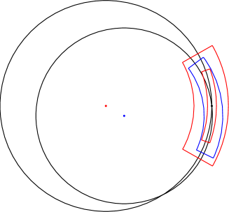
Figure 1. Illustration of the conclusion of Proposition 9.

∎

Corollary 4.

Let $\Omega^{(v)}$ be a $\delta,\tau$-rectangle contained in $\overline{\Omega}^{(w)}$, an $A^{2}\delta,A\tau$-rectangle. Then $v\in\mathcal{C}_{A_{1}A^{5}\delta}(\overline{\Omega})$.

Proof.

By Proposition 9, and since $\overline{\Omega}$ is an $A^{2}\delta,A\tau$-rectangle, by definition, $v\in\mathcal{C}_{A_{1}A^{5}\delta}(\overline{\Omega})$. ∎

Now we are ready to give the proof that being comparable is almost a transitive relation. For the purpose of stating it succinctly, if $\Omega,\Omega^{\prime}$ are $A$-comparable, we write $\Omega\asymp_{A}\Omega^{\prime}$.

Proposition 10 (Almost-transitivity).

There is an absolute constant $C>1$ such that if $\Omega_{1}\asymp_{A}\Omega_{2}$ and $\Omega_{2}\asymp_{A}\Omega_{3}$, then $\Omega_{1}\asymp_{A^{C}}\Omega_{3}$.

Proof.

Suppose the core circles of $\Omega_{i}$ are $v_{i}\in Q$, $i=1,2,3$. Consider the radial projection $\pi\colon\mathbb{R}^{2}\setminus\{v_{2}^{\prime}\}\to C_{v_{2}}$ onto $C_{v_{2}}$. By assumption, $\pi(\Omega_{1}\cup\Omega_{3})$ is contained in an arc of length $\sim A\tau$ containing the core arc of $\Omega_{2}$. Therefore, it suffices to show that $\Omega_{1}$ and $\Omega_{3}$ are contained in $C_{A^{O(1)}\delta,v_{2}}$, as this will imply that $\Omega_{1}\cup\Omega_{3}$ is contained in an $A^{O(1)}\delta,O(A)\tau$-rectangle, which is the desired relation.

Let $\overline{\Omega}_{12}\supset\Omega_{1}\cup\Omega_{2}$ and $\overline{\Omega}_{23}\supset\Omega_{2}\cup\Omega_{3}$ be the rectangles coming from the assumption $\Omega_{1}\asymp_{A}\Omega_{2}$, $\Omega_{2}\asymp_{A}\Omega_{3}$. By Proposition 9, $\overline{\Omega}_{12}\cup\overline{\Omega}_{23}\subset C_{A^{O(1)}\delta,v_{2}}$, which finishes the proof. ∎

To turn statements about comparable rectangles into statements about nearly overlapping lightplanks, we need a lemma that relates different lightlike coordinate systems.

Proposition 11.

Let $\mathcal{E}=e_{s},e_{m},e_{l}$ and $\overline{\mathcal{E}}=\bar{e}_{s},\bar{e}_{m},\bar{e}_{l}$ be two lightlike bases of $\mathbb{R}^{3}$. If $\theta=\angle e_{m},\bar{e}_{m}$, then the following relationship holds between $\mathcal{E}$ and $\overline{\mathcal{E}}$:

$$\begin{matrix}\bar{e}_{s}&=&-\frac{\sin\theta}{\sqrt{2}}e_{m}&+&\frac{\cos\theta-1}{2}e_{l}&+&\frac{\cos\theta+1}{2}e_{s},\\ \bar{e}_{m}&=&\cos\theta\,e_{m}&+&\frac{\sin\theta}{\sqrt{2}}e_{l}&+&\frac{\sin\theta}{\sqrt{2}}e_{s},\\ \bar{e}_{l}&=&-\frac{\sin\theta}{\sqrt{2}}e_{m}&+&\frac{\cos\theta+1}{2}e_{l}&+&\frac{\cos\theta-1}{2}e_{s}.\end{matrix}$$

Proof.

By rotating our coordinate system if necessary, we may assume that in our chosen coordinates, we have

$$e_{m}=\begin{pmatrix}0\\ 1\\ 0\end{pmatrix},e_{l}=\frac{1}{\sqrt{2}}\begin{pmatrix}-1\\ 0\\ 1\end{pmatrix},e_{s}=\frac{1}{\sqrt{2}}\begin{pmatrix}-1\\ 0\\ -1\end{pmatrix}.$$

By our assumption that $\angle e_{m},\bar{e}_{m}=\theta$, we can write

$$\bar{e}_{m}=\begin{pmatrix}-\sin\theta\\ \cos\theta\\ 0\end{pmatrix},\bar{e}_{l}=\frac{1}{\sqrt{2}}\begin{pmatrix}-\cos\theta\\ -\sin\theta\\ 1\end{pmatrix},\bar{e}_{s}=\frac{1}{\sqrt{2}}\begin{pmatrix}-\cos\theta\\ -\sin\theta\\ -1\end{pmatrix}.$$

As the bases $\mathcal{E}$, $\overline{\mathcal{E}}$ are orthonormal, the conclusion follows by computing the 9 inner products $\langle\bar{e}_{s},e_{m}\rangle$, $\langle\bar{e}_{s},e_{l}\rangle$, etc. ∎

In the next proposition, we do not make a serious attempt to optimize the exponent of $A$, since the only point is to establish a bound of the form $A^{C}\tau$ for an absolute $C$.

Proposition 12.

Suppose $\Omega^{(v)}\subset\overline{\Omega}^{(w)}$, where $\Omega^{(v)}$ is a $\delta,\tau$-rectangle, and $\overline{\Omega}^{(w)}$ is an $A^{2}\delta,A\tau$-rectangle. Let $a,\bar{a}$ be the center points of $\Omega^{(v)}$ and $\overline{\Omega}^{(w)}$, respectively, and let $e_{m},\bar{e}_{m}$ be the positively oriented tangent vectors to $v,w$ at the points $a,\bar{a}$, respectively. Then $\angle e_{m},\bar{e}_{m}\lesssim A^{4}\tau$.

Proof.

Let $d=d(v,w)$, $\Delta=\Delta(v,w)$, and let $\gamma,\overline{\gamma}$ denote the core arcs of $\Omega,\overline{\Omega}$. We make the same simplifying technical assumption as in Proposition 9, that there exists a point $x\in\gamma\cap\overline{\gamma}$ to make use of Proposition 8. To remove this assumption, we note by replacing $v$ with a concentric circle of a slightly smaller or larger radius, we can arrange for $\gamma\cap\overline{\gamma}\neq\emptyset$, while keeping $\angle e_{m},\bar{e}_{m}$ and $\Omega^{(v)}\subset\overline{\Omega}^{(w)}$. By Proposition 8, the angle between $v$ and $w$ at $x$ is $\sim\sqrt{d\Delta}$.

By assumption $\Omega^{(v)}\subset\overline{\Omega}^{(w)}$,

$$|C_{A^{2}\delta,v}\cap C_{A^{2}\delta,w}|\geq|\Omega|\sim\delta\tau.$$

On the other hand, by Lemma 1,

$$|C_{A^{2}\delta,v}\cap C_{A^{2}\delta,w}|\lesssim\frac{(A^{2}\delta)^{2}}{\sqrt{(d+A^{2}\delta)(\Delta+A^{2}\delta)}}.$$

Rearranging the inequality and using our a priori assumption $\delta^{1/2}\leq\tau$ gives

$$\sqrt{d\Delta}\lesssim A^{4}\delta\tau^{-1}\leq A^{4}\tau.$$

Finally, because $\mathrm{dist}(a,x)+\mathrm{dist}(x,\bar{a})\lesssim A\tau$, by comparing angles at $a$ and $\bar{a}$, we conclude $\angle e_{m},\bar{e}_{m}=O(A^{4})\tau+O(A)\tau=O(A^{4})\tau$. ∎

Proposition 13.

Suppose $\Omega^{(v)}\subset\overline{\Omega}^{(w)}$, where $\Omega^{(v)}$ is a $\delta,\tau$-rectangle, and $\overline{\Omega}^{(w)}$ is an $A^{2}\delta,A\tau$-rectangle. Let $P=\mathcal{C}_{\delta}(\Omega)$ and $\overline{P}=\mathcal{C}_{A^{2}\delta}(\overline{\Omega})$. Then for an absolute constant $C>1$, $P\subset A^{C}\overline{P}$.

Proof.

Let $\mathcal{E}=e_{s},e_{m},e_{l}$ and $\overline{\mathcal{E}}=\bar{e}_{s},\bar{e}_{m},\bar{e}_{l}$ be the lightlike bases associated with the lightplanks $P$ and $\overline{P}$, respectively. Let $\theta=\angle e_{m},\bar{e}_{m}$. Because $\Omega\subset C_{A^{2}\delta,w}$, $w\in\mathcal{C}_{A^{2}\delta}(\Omega)$, which is contained in an $A^{2}$-dilation of $P$ by Proposition 6.

Hence, by Proposition 11, in $\mathcal{E}$, we have

$$\begin{matrix}|\langle v-w,\bar{e}_{s}\rangle|&\leq&|\langle v-w,e_{s}\rangle|&+&O(\theta)|\langle v-w,e_{m}\rangle|&+&O(\theta^{2})|\langle v-w,e_{l}\rangle|\\ &\leq&A^{2}\delta&+&O(\theta)A^{2}\delta\tau^{-1}&+&O(\theta^{2})A^{2}\delta\tau^{-2}.\end{matrix}$$

By Proposition 12, $|\theta|\lesssim A^{4}\tau$, so $|\langle v-w,\bar{e}_{s}\rangle|\lesssim A^{10}\delta$. Analogous considerations using Proposition 11 and $|\theta|\lesssim A^{4}\tau$ show $|\langle v-w,\bar{e}_{m}\rangle|\lesssim A^{6}\delta\tau^{-1}$ and $|\langle v-w,\bar{e}_{l}\rangle|\lesssim A^{2}\delta\tau^{-2}$. Since $\overline{P}$ is a $A^{2}\delta\times A\delta\tau^{-1}\times\delta\tau^{-2}$-lightplank, we find $v\in CA^{8}\overline{P}$. Now it suffices to prove that for any $x\in P=P^{(v)}$, the inequalities

$$|\langle x-v,\bar{e}_{s}\rangle| \lesssim A^{C}\delta$$

$$|\langle x-v,\bar{e}_{m}\rangle| \lesssim A^{C}\delta\tau^{-1}$$

$$|\langle x-v,\bar{e}_{l}\rangle| \lesssim A^{C}\delta\tau^{-2}$$

all hold. We provide the details to estimate $|\langle x-v,\bar{e}_{s}\rangle|$ as the proofs of the remaining inequalities are entirely analogous. By Proposition 11 again, we have

(4) $$|\langle x-v,\bar{e}_{s}\rangle|\lesssim O(1)|\langle x-v,e_{s}\rangle|+O(\theta)|\langle x-v,e_{m}\rangle|+O(\theta^{2})|\langle x-v,e_{l}\rangle|.$$

Since $x\in P$, in the lightlike coordinate system $\mathcal{E}$, we have

$$|\langle x-v,e_{s}\rangle| \lesssim\delta$$

$$|\langle x-v,e_{m}\rangle| \lesssim\delta\tau^{-1}$$

$$|\langle x-v,e_{l}\rangle| \lesssim\delta\tau^{-2}.$$

Substituting these estimates into (4) with $|\theta|\lesssim A^{4}\tau$, we obtain

$$|\langle x-v,\bar{e}_{s}\rangle|\lesssim A^{8}\delta.$$

Using the remaining two relations from Proposition 11 provides the required estimates for $|\langle x-v,\bar{e}_{m}\rangle|$ and $|\langle x-v,\bar{e}_{l}\rangle|$, and this finishes the proof. ∎

In the other direction, assuming $P\subset\overline{P}\subset\mathbb{R}^{2}\times[1-\alpha_{0},1+\alpha_{0}]$ for two lightplanks, we can say something about the corresponding dual rectangles.

Proposition 14.

Suppose $P^{(v)}\subset\overline{P}^{(w)}\subset\mathbb{R}^{2}\times[1-\alpha_{0},1+\alpha_{0}]$, where $P^{(v)}$ is a $\delta\times\delta\tau^{-1}\times\delta\tau^{-2}$-rectangle centered on $v$, and $\overline{P}^{(w)}$ is an $A^{2}\delta\times A\delta\tau^{-1}\times\delta\tau^{-2}$-lightplank centered on $w$. Let $\Omega^{(v)}=\mathcal{V}_{\delta}(P)$ and $\overline{\Omega}^{(w)}=\mathcal{V}_{\delta}(\overline{P})$. Then there is an $A^{6}\delta,A^{2}\tau$-rectangle containing $\Omega\cup\overline{\Omega}$.

Proof.

By Corollary 2, $\Omega^{(v)}\subset\overline{\Omega}^{(w)}$, where $\Omega$ is a $\delta,\tau$-rectangle, and $\overline{\Omega}$ is an $A^{2}\delta,A\tau$-rectangle. By Corollary 4, $\overline{\Omega}\subset C_{A^{5}\delta,v}$, so it suffices to prove that the angle $\theta:=\angle e_{m},\bar{e}_{m}$ between the intermediate edges of the lightplanks $P,\overline{P}$, respectively is at most $O(A^{2})\tau$. If this is done, it shows that $\Omega\cup\overline{\Omega}$ is contained in an $A^{5}\delta,A^{2}\tau$-rectangle. Consider the plane $\Pi$ containing the lower $A\delta\tau^{-1}\times A^{2}\delta$ face of the lightplank $\overline{P}$ (see Figure 2). Considering the edges of $P,\overline{P}$ in the plane $\Pi$, we have

$$\theta\sim\sin\theta\leq\frac{A^{2}\delta}{\delta\tau^{-1}}=A^{2}\tau,$$

and this finishes the proof.

Figure 2. Bottom faces of the lightplanks $P,\overline{P}$ in the plane $\Pi$.

∎

The next proposition combines the last few propositions to characterize comparability of $\delta,\tau$-rectangles in terms of an analogous statement concerning their dual lightplanks. In the statement of the proposition, the absolute constant $C$ can vary within the same line, but the only important point is that in each instance the constant is absolute.

Proposition 15 (Comparability dictionary).

Suppose $\Omega_{1},\Omega_{2}$ are $\delta,\tau$-rectangles in the plane with corresponding lightplanks $P_{1},P_{2}\subset\mathbb{R}^{2}\times[1-\alpha_{0},1+\alpha_{0}]$. If $\Omega_{1},\Omega_{2}$ are $A$-comparable, then there is a $A^{C}\delta\times A^{C}\delta\tau^{-1}\times A^{C}\delta\tau^{-2}$-lightplank $\overline{P}$ containing $P_{1}\cup P_{2}$. Conversely, if $P_{1}\cup P_{2}\subset\overline{P}$ for some $A^{C}\delta\times A^{C}\delta\tau^{-1}\times A^{C}\delta\tau^{-2}$-lightplank $\overline{P}$, then $\Omega_{1},\Omega_{2}$ are $A^{C}$-comparable.

Proof.

Suppose that $\Omega_{1},\Omega_{2}$ are $A$-comparable, and let $\overline{\Omega}$ be an $A^{2}\delta,A\tau$-rectangle containing $\Omega_{1}\cup\Omega_{2}$, and $\overline{P}=\mathcal{C}_{A^{2}\delta}(\overline{\Omega})$ its dual lightplank. By Proposition 13, $P_{1}\cup P_{2}$ is contained in an $A^{C}$-dilation of $\overline{P}$.

Conversely, if $P_{1}\cup P_{2}\subset\overline{P}$ for an $A^{C}\delta\times A^{C}\delta\tau^{-1}\times A^{C}\delta\tau^{-2}$-lightplank $\overline{P}$, then by Proposition 14, $\Omega_{1}\cup\Omega_{2}$ is contained in a single $A^{C}\delta,A^{C}\tau$-rectangle, so $\Omega_{1},\Omega_{2}$ are $A^{C}$-comparable. ∎

4.3. Packing rectangles

The next proposition is a minor refinement of Lemma 1.2 in [6]. The refinement comes in the form of being more explicit about the shape of the constant, and the only important point is it is at most $(A_{0}A)^{C}$ for an absolute constant $C>1$ (rather than an intolerable exponential growth, e.g. $e^{A_{0}A}$). We remark that much of the work we have done in this section was for the sake of having a concise proof of this proposition.

Proposition 16 (Packing).

For any $A_{0}\geq 1$, the number of pairwise $A$-incomparable $\delta,\tau$-rectangles contained in an $A_{0}A^{2}\delta,A_{0}A\tau$-rectangle is $\lesssim(A_{0}A)^{C}$.

Proof.

Let $\overline{\Omega}$ be an $A_{0}A^{2}\delta,A_{0}A\tau$-rectangle. By covering $\overline{\Omega}$ with $O(A_{0})$ finitely overlapping $A_{0}A^{2}\delta,A\tau$-rectangles, it suffices to check that the number of pairwise $A$-incomparable $\delta,\tau$-rectangles contained in an $A_{0}A^{2}\delta,A\tau$-rectangle, that we also denote by $\overline{\Omega}$, is at most $C(A_{0}A)^{C}$.

Let $\{\Omega^{(v_{i})}\}_{i=1}^{M}$ be a maximal pairwise $A$-incomparable collection of $\delta,\tau$-rectangles contained in $\overline{\Omega}^{(o)}$.

Let $\overline{\mathcal{E}}=\bar{e}_{s},\bar{e}_{m},\bar{e}_{l}$ be the lightlike basis associated to the lightplank $\overline{P}$ with center $o$. By Proposition 13, for each $i$, $v_{i}\in(A_{0}A)^{C}\overline{P}$, so each of the following inequalities holds for every $i,j\in\{1,\dots,M\}$:

• $|\langle v_{i}-v_{j},\bar{e}_{s}\rangle|\lesssim(A_{0}A)^{C}\delta$

• $|\langle v_{i}-v_{j},\bar{e}_{m}\rangle|\lesssim(A_{0}A)^{C}\delta\tau^{-1}$

• $|\langle v_{i}-v_{j},\bar{e}_{l}\rangle|\lesssim(A_{0}A)^{C}\delta\tau^{-2}$.

As the circles $v_{1},\dots,v_{M}$ contained in $(A_{0}A)^{C}\overline{P}$ are $A$-incomparable, for each $i\neq j$, at least one of the following inequalities must hold by Proposition 15:

• $|\langle v_{i}-v_{j},\bar{e}_{s}\rangle|\gg A^{C}\delta$

• $|\langle v_{i}-v_{j},\bar{e}_{m}\rangle|\gg A^{C}\delta\tau^{-1}$

• $|\langle v_{i}-v_{j},\bar{e}_{l}\rangle|\gg A^{C}\delta\tau^{-2}$.

Therefore, $M\lesssim(A_{0}A)^{C}$, and the claim is proved. ∎

5. Application of the maximal function estimate

In this section, we show how to combine the geometric considerations from Section 4 with the maximal function estimate to count pairs of nearly internally tangent circles. Throughout, assume $X\subset Q$ is a set of at most $R=\delta^{-1}$ circles, let $\epsilon>0$ be fixed, and $\delta<\delta_{0}(\epsilon)$. We define a family of multiplicity functions by

$$g_{\lambda\delta}(y)=\sum_{x\in X}C_{\lambda\delta,x}(y),\qquad y\in\mathbb{R}^{2},\lambda\geq 1.$$

Throughout, we work with $\lambda\lessapprox 1$.

Proposition 17.

There is an absolute constant $C\geq 1$ such that the following holds. Let $\mathcal{R}$ be an $A$-incomparable collection of $\delta,\tau$-rectangles contained in $\bigcup_{x\in X}C_{\delta,x}$. For each $x\in X$, and each $\lambda\geq A$,

$$\sum_{\begin{subarray}{c}\Omega\in\mathcal{R}\\ x\in\mathcal{C}_{\lambda\delta}(\Omega)\end{subarray}}\Omega(y)\lesssim\lambda^{C}C_{\lambda\delta,x}(y).$$

Proof.

For each fixed $y\in\mathbb{R}^{2}$, the $\Omega\in\mathcal{R}$ which contain $y$ and which are contained in $C_{\lambda\delta,x}$ are contained in a $\lambda\delta,C\tau$-rectangle. As the $\Omega\in\mathcal{R}$ are pairwise $A$-incomparable, by Proposition 16, the number of such $\Omega$ is at most $\lambda^{C}$ for some absolute constant $C$. ∎

Given $\lambda\geq 1$, and a $\delta,\tau$-rectangle $\Omega$, we let

$$\nu_{\lambda\delta}(\Omega)=|X\cap\mathcal{C}_{\lambda\delta}(\Omega)|.$$

For $\lambda\approx 1$, the number $\nu_{\lambda\delta}(\Omega)$ counts the number of circles in $X$ which contain an arc of length $\approx\tau$ that is $\approx\delta$-close to the true core arc of $\Omega$. As we saw throughout Section 4, in addition to $\delta,\tau$-rectangles, we have to consider slightly larger rectangles. For this reason we have to define and work with the numbers $\nu_{\lambda\delta}(\Omega)$ for $\lambda\approx 1$.

Proposition 18.

If $\mathcal{R}$ is a pairwise $A$-incomparable collection of $\delta,\tau$-rectangles contained in $\bigcup_{x\in X}C_{\delta,x}$ and $\lambda\geq A$, then

$$\sum_{\Omega\in\mathcal{R}}\nu_{\lambda\delta}(\Omega)\Omega(y)\lesssim\lambda^{C}g_{\lambda\delta}(y).$$

Proof.

For each $\Omega\in\mathcal{R}$ and each $\lambda\geq 1$,

$$\nu_{\lambda\delta}(\Omega)\Omega(y)=\sum_{x\in\mathcal{C}_{\lambda\delta}(\Omega)}\Omega(y)C_{\lambda\delta,x}(y),$$

by the definition of $\mathcal{C}_{\lambda\delta}(\Omega)$. Summing over $\Omega\in\mathcal{R}$ and changing the order of summation,

$$\sum_{\Omega\in\mathcal{R}}\nu_{\lambda\delta}(\Omega)\Omega(y) =\sum_{\Omega\in\mathcal{R}}\sum_{x\in\mathcal{C}_{\lambda\delta}(\Omega)}\Omega(y)C_{\lambda\delta,x}(y)$$

$$=\sum_{x\in X}C_{\lambda\delta,x}(y)\sum_{\begin{subarray}{c}\Omega\in\mathcal{R}\\ x\in\mathcal{C}_{\lambda\delta}(\Omega)\end{subarray}}\Omega(y).$$

By Proposition 17, for each $\lambda\geq A$, the inner sum is bounded by $\lambda^{C}C_{\lambda\delta,x}(y)$. Combining this with the definition of $g_{\lambda\delta}(y)$ finishes the proof. ∎

For $\delta^{1/2}<\tau<\delta^{\epsilon}$, let

$$\gamma_{\tau}=\max\{|X\cap\mathcal{C}_{\delta}(\Omega)|:\Omega\subset\mathbb{R}^{2}\ \text{is a $\delta,\tau$-rectangle}\},$$

or equivalently by Corollary 2,

$$\gamma_{\tau}=\max\{|X\cap P|:P\subset Q\ \text{is a lightplank of dimensions\ }\delta\times\delta\tau^{-1}\times\delta\tau^{-2}\}.$$

Proposition 19.

If $\Omega$ is a $\delta,\tau$-rectangle, then for each $\lambda\approx 1$,

$$\nu_{\lambda\delta}(\Omega)\lessapprox\gamma_{\tau}.$$

Proof.

Notation aside, the proposition says that the number of points in $X$ contained in a given lightplank with dimensions slightly larger than $\delta\times\delta\tau^{-1}\times\delta\tau^{-2}$, as quantified by $\lambda$, is not much more than the maximal number of points of $X$ contained in a $\delta\times\delta\tau^{-1}\times\delta\tau^{-2}$-lightplank. The proof is a routine covering and pigeonholing argument, so we omit the details. ∎

For a dyadic number $M\in[1,\gamma_{\tau}]$ a number $\lambda\approx 1$, and a collection $\mathcal{R}$ of $\delta,\tau$-rectangles, let

$$\mathcal{R}_{M,\lambda}=\{\Omega\in\mathcal{R}:\nu_{\lambda\delta}(\Omega)\sim M\}.$$

The next proposition is the culmination of this subsection which will ultimately allow us to estimate pairs of nearly internally tangent circles. Recall the notation $Q=[0,2\alpha_{0}]^{2}\times[1-\alpha_{0},1+\alpha_{0}]\subset\mathbb{R}^{3}$.

Proposition 20.

Suppose that $X\subset Q$ is a set of at most $R$ circles in $Q$ either having one radius per interval of length $\sim\delta$, or else satisfying the 1-dimensional Frostman condition

$$|X\cap B(x_{0},r)|\lesssim_{\epsilon}\delta^{-\epsilon}(r/\delta),\ \qquad x_{0}\in Q,r\geq\delta.$$

If $\mathcal{R}$ is any pairwise $A$-incomparable collection of $\delta,\tau$-rectangles contained in $\bigcup_{x\in X}C_{\delta,x}$, then for each $M\in[1,\gamma_{\tau}]$ and $A\leq\lambda\lessapprox 1$,

$$M^{3/2}|\mathcal{R}_{M,\lambda}|\lesssim\delta^{-C\epsilon}\tau^{-1}|X|.$$

Proof.

By Proposition 18, if $\lambda\geq A$, we have

$$\lambda^{C}g_{\lambda\delta}(y)\gtrsim\sum_{\Omega\in\mathcal{R}}\nu_{\lambda\delta}(\Omega)\Omega(y).$$

We organize the sum on the right-hand side by the dyadic level sets of $\nu_{\lambda\delta}(\Omega)$, noting that $\nu_{\lambda\delta}(\Omega)\lessapprox\gamma_{\tau}$:

$$\lambda^{C}g_{\lambda\delta}(y)\gtrsim\sum_{\begin{subarray}{c}1<M<\gamma_{\tau}\\ M\ \text{dyadic}\end{subarray}}M\sum_{\Omega\in\mathcal{R}_{M,\lambda}}\Omega(y).$$

By Example 1, or the estimate of Theorem 6, and the embedding $\ell^{1}\hookrightarrow\ell^{3/2}$,

$$\delta^{-C\epsilon}\cdot\delta|X|\gtrsim\lambda^{C}\int g_{\lambda\delta}^{3/2}\gtrsim M^{3/2}|\mathcal{R}_{M,\lambda}|\cdot|\Omega|.$$

Dividing by $|\Omega|\sim\delta\tau$ finishes the proof. ∎

In the next subsection we will specialize the value of $\tau$ for our application.

5.1. Nearly lightlike pairs

Fix a set $X\subset Q$ of circles satisfying the Frostman condition

$$|X\cap B^{3}(x_{0},r)|\lesssim_{\epsilon}\delta^{-\epsilon}(r/\delta)\quad\text{for all $x_{0}\in Q$, $r\geq\delta$}.$$

In particular, $|X|\lessapprox R$, though $|X|$ can be much smaller. For dyadic numbers $\delta<\Delta\leq D<1$, define a collection

$$\mathcal{L}_{D,\Delta}=\{(x,y)\in X\times X:d(x,y)\sim D,\Delta(x,y)\sim\Delta\}.$$

We will be interested in the cardinality of the collection $\mathcal{L}_{D,\Delta}$ when $D>\delta^{1-C\epsilon}$ and $\Delta<\delta^{1-\epsilon}$ as this is the only range of the parameters where we require a nontrivial estimate of $|\mathcal{L}_{D,\Delta}|$. We will refer to a pair $(x,y)\in\mathcal{L}_{D,\Delta}$ as nearly lightlike when $\Delta<\delta^{1-\epsilon}$. In order to estimate the number of nearly lightlike pairs, we will ultimately use Proposition 20. Let $\tau_{D}=\delta^{1/2}D^{-1/2}$.

Definition 7.

We say two circles $C_{v},C_{w}$ are $\gtrapprox\delta,\tau$-tangent if there are $\approx 1$-comparable $\delta,\tau$-rectangles $\Omega^{(v)}\subset C_{\delta,v}$, $\Omega^{(w)}\subset C_{\delta,w}$.

Proposition 21.

If $(v,w)\in\mathcal{L}_{D,\Delta}$ for $D\gg\delta$ and $\Delta\lessapprox\delta$, then $C_{v},C_{w}$ are $\gtrapprox\delta,\tau_{D}$-tangent.

Proof.

Suppose $D\gg\delta$, $\Delta\lessapprox\delta$, and $(v,w)\in\mathcal{L}_{D,\Delta}$. We will find a lightplank $P\subset\mathbb{R}^{2}\times[1-\alpha_{0},1+\alpha_{0}]$ of dimensions $\approx\delta\times\delta\tau_{D}^{-1}\times\delta\tau_{D}^{-2}$ such that both $v,w\in P$. By duality, for an appropriate $A\approx 1$, $\Omega^{(v)}:=\mathcal{V}_{A\delta}(P)\cap C_{\delta,v}$ and $\Omega^{(w)}:=\mathcal{V}_{A\delta}(P)\cap C_{\delta,w}$ are $\approx 1$-comparable $\delta,\tau_{D}$-rectangles contained in $C_{\delta,v}$ and $C_{\delta,w}$, respectively, so this will finish the proof.

Let $w_{0}\in\Gamma_{v}$ be the nearest point to $w$ in the lightcone with vertex $v$. By definition, $v-w_{0}$ is a lightlike vector, and since $\delta\ll D$, we have $|v-w_{0}|\sim|v-w|\sim D$ and $|w_{0}-w|=\Delta(v,w)\lessapprox\delta$. Let $e_{m}$ be a unit tangent vector to the $x_{3}$-slice of $\Gamma_{v}$ containing $w_{0}$; let $e_{l}$ be the unit vector in the direction $v-w_{0}$, and let $e_{s}$ be such that $\mathcal{E}=e_{l},e_{m},e_{s}$ is an orthonormal basis. To show that $v,w$ both belong to a common lightplank of the required dimensions, it suffices to show that

• $|\langle v-w,e_{l}\rangle|\lessapprox\delta\tau_{D}^{-2}$,

• $|\langle v-w,e_{m}\rangle|\lessapprox\delta\tau_{D}^{-1}$, and

• $|\langle v-w,e_{s}\rangle|\lessapprox\delta$.

Since $\delta\tau_{D}^{-2}=D\sim|\langle v-w,e_{l}\rangle|$, and $\Delta(v,w)=|w-w_{0}|\sim|\langle v-w,e_{s}\rangle|\lessapprox\delta$, only point (ii) needs elaboration. But by elementary geometry considerations, this is a simple consequence of the assumption $d(v,w)\sim D$ and $\Delta(v,w)\lessapprox\delta$. ∎

Proposition 22.

There is an absolute constant $C>1$ so that the following holds. If $(v,w)\in\mathcal{L}_{D,\Delta}$ and $\mathcal{R}$ is a maximal pairwise $A$-incomparable collection of $\delta,\tau_{D}$-rectangles contained in $\bigcup_{x\in X}C_{\delta,x}$, then there exists $\Omega\in\mathcal{R}$ so that $v,w\in\mathcal{C}_{A^{C}\delta}(\Omega)$.

Proof.

By Proposition 21, there are $\approx 1$-comparable $\delta,\tau_{D}$ rectangles $\Omega^{(v)},\Omega^{(w)}$ in $C_{\delta,v},C_{\delta,w}$ respectively. By maximality of $\mathcal{R}$ with respect to $A$-incomparability, there is some $\Omega\in\mathcal{R}$ such that $\Omega^{(v)}$ (say) is $A$-comparable to $\Omega$. This shows that $v\in\mathcal{C}_{\lambda\delta}(\Omega)$ for some $\lambda=O(A^{C})$.

As $\Omega^{(v)}$ and $\Omega^{(w)}$ are $A$-comparable, by almost-transitivity (Proposition 10), $\Omega$ and $\Omega^{(w)}$ are $\lambda^{C}=A^{O(1)}$-comparable. Hence $w\in\mathcal{C}_{\lambda^{C}\delta}(\Omega)$ for a large enough absolute constant $C$, and the claim is proved as $v\in\mathcal{C}_{\lambda\delta}(\Omega)\subset\mathcal{C}_{\lambda^{C}\delta}(\Omega)$. ∎

Proposition 23.

If $\Delta\lesssim\delta^{1-\epsilon}$, and $D>\delta^{1-C\epsilon}$ then $|\mathcal{L}_{D,\Delta}|\lessapprox\gamma_{\tau_{D}}^{1/2}(RD)^{1/2}|X|$.

Proof.

Let $A\approx 1$ be a parameter (take $A=\delta^{-\epsilon}$ for definiteness), and fix an arbitrary maximal pairwise $A$-incomparable collection $\mathcal{R}$ of $\delta,\tau_{D}$-rectangles contained in $\bigcup_{x\in X}C_{\delta,x}$.

By Proposition 22, for a given $(v,w)\in\mathcal{L}_{D,\Delta}$, we can find a rectangle $\Omega\in\mathcal{R}$ such that $v,w\in\mathcal{C}_{\lambda\delta}(\Omega)$ for some $\lambda=A^{O(1)}$, and we can write

$$\mathcal{L}_{D,\Delta}\subset\bigcup_{\Omega\in\mathcal{R}}\{(v,w)\in X\times X:v,w\in\mathcal{C}_{\lambda\delta}(\Omega)\}.$$

By the union bound,

(5) $$|\mathcal{L}_{D,\Delta}|\leq\sum_{\Omega\in\mathcal{R}}|X\cap\mathcal{C}_{\lambda\delta}(\Omega)|^{2}=:\sum_{\Omega\in\mathcal{R}}\nu_{\lambda\delta}(\Omega)^{2}.$$

Recall that by Proposition 19, $\nu_{\lambda\delta}(\Omega)\lessapprox\gamma_{\tau_{D}}$. We organize the last sum on the right-hand side of (5) by the dyadic value of $\nu_{\lambda\delta}(\Omega)$, up to $\gamma_{\tau_{D}}$, the same as we did in Proposition 20. Letting $\mathcal{R}_{M,\lambda}=\{\Omega\in\mathcal{R}:\nu_{\lambda\delta}(\Omega)\sim M\}$, we estimate (5) by

$$\sum_{\begin{subarray}{c}1<M<\gamma_{\tau_{D}}\\ M\ \text{dyadic}\end{subarray}}M^{2}|\mathcal{R}_{M,\lambda}|.$$

By Proposition 20, for each $M$, $M^{3/2}|\mathcal{R}_{M,\lambda}|\lessapprox\tau_{D}^{-1}|X|=(RD)^{\frac{1}{2}}|X|$. As $\gamma_{\tau_{D}}\leq\delta^{-1}$ a priori, there are $\approx 1$-many values of $M$ in the sum, so we have shown $|\mathcal{L}_{D,\Delta}|\lessapprox\gamma_{\tau_{D}}^{1/2}(RD)^{1/2}|X|$. This finishes the proof. ∎

6. Proof of Theorem 4 and sharpness

Besides the geometric considerations of Sections 4 and 5, the main ingredient we need for the proof of Theorem 4 is a stationary phase estimate for the Fourier transform of $\sigma$, a smooth surface measure on the cone segment. Recall $\Gamma_{0}=\{(x^{\prime},x_{3}):||x^{\prime}|-|x_{3}||=0\}$ is the lightcone in $\mathbb{R}^{3}$ with vertex 0. We state the version of the estimate we will use in the proof of Theorem 4 here. The proof of this lemma is contained in the appendix.

Lemma 2.

Let $\sigma$ be a smooth compactly supported surface measure in $\mathbb{C}one^{2}$. For any $\epsilon>0$, there is a constant $C_{\epsilon}$ so that

$$|\widecheck{\sigma}(x)|\leq C_{\epsilon}\frac{1}{(1+|x|)^{\frac{1}{2}-\epsilon}}\frac{1}{(1+d(x,\Gamma_{0}))^{100\epsilon^{-1}}}.$$

Now we are ready to give the proof of Theorem 4, whose statement we recollect here.

Theorem 7.

For each $\epsilon>0$, there is a constant $C_{\epsilon}$ so the following holds for each $R>1$. Suppose $\nu$ is a measure that agrees with the Lebesgue measure on a union of lattice unit cubes $X\subset[0,R]^{2}\times[R,2R]=:B_{R}$ and satisfies the 1-dimensional Frostman condition

$$\nu(B(x_{0},r))\lesssim r,\qquad x_{0}\in\mathbb{R}^{3},r>1.$$

Let $\mathbf{P}(\nu)$ be the quantity

$$\mathbf{P}(\nu)=\max\{\nu(P):P\ \text{is a lightplank of dimensions $1\times R^{1/2}\times R$}\}.$$

Then the estimate

$$\int|\widehat{\nu}|^{2}\,d\sigma\leq C_{\epsilon}R^{\epsilon}\,\mathbf{P}(\nu)^{1/2}\|\nu\|$$

holds, where $\|\nu\|:=\nu(B_{R})=|X|$ is the total mass of $\nu$.

Proof.

By duality and Fourier transform properties,

$$\|\widehat{\nu}\|_{L^{2}(d\sigma)}^{2}=\int\widehat{\nu}\overline{\widehat{\nu}}\,d\sigma=\iint_{B_{R}\times B_{R}}\widecheck{\sigma}(x-y)\,d\nu(x)d\nu(y).$$

We will estimate this integral by dividing the domain of integration into regions where we have good control on the integrand. For instance,

$$\iint\widecheck{\sigma}(x-y)\,d\nu(x)d\nu(y) =\iint_{|x-y|\leq R^{10\epsilon}}\widecheck{\sigma}(x-y)\,d\nu(x)d\nu(y)+\iint_{|x-y|>R^{10\epsilon}}\widecheck{\sigma}(x-y)\,d\nu(x)d\nu(y)$$

$$=:I+II.$$

Because $|\widecheck{\sigma}|\lesssim 1$ everywhere, we can estimate $|I|\lesssim R^{10\epsilon}|X|$. To estimate $|II|$, by slight abuse of notation, let $X=\{(a_{i},r_{i}):i=1,\dots,|X|\}$ be the collection of centers of the cubes in the support of $\nu$. For any $x\in B_{R}$, we have a corresponding point $\tilde{x}\in B_{1}$ defined by $\tilde{x}=R^{-1}x$. For each pair $x,y\in X$, we consider the numbers

$$d(\tilde{x},\tilde{y})=R^{-1}|x-y|\quad\text{and}\quad\Delta(\tilde{x},\tilde{y})=R^{-1}||x^{\prime}-y^{\prime}|-|x_{3}-y_{3}||.$$

These are simply the scaled down values of $d(x,y)$ and $\Delta(x,y)$. We write things this way to use the results of Section 5 which are phrased at scales $\leq 1$. For any dyadic number $\delta^{1-10\epsilon}<D<1$, we let

$$\mathcal{L}_{D,\lessapprox\delta} =\{(x,y)\in X\times X:d(\tilde{x},\tilde{y})\sim D,\Delta(\tilde{x},\tilde{y})\leq\delta^{1-\epsilon}\}$$

$$\mathcal{L}_{D,\gg\delta} =\{(x,y)\in X\times X:d(\tilde{x},\tilde{y})\sim D,\Delta(\tilde{x},\tilde{y})>\delta^{1-\epsilon}\}.$$

We let $\mathcal{L}_{D,\lessapprox\delta}^{1},\mathcal{L}_{D,\gg\delta}^{1}$ denote the $1$-neighborhoods of $\mathcal{L}_{D,\lessapprox\delta},\mathcal{L}_{D,\gg\delta}$ in $\mathbb{R}^{3}\times\mathbb{R}^{3}$, respectively. We organize the integral $II$ by writing

$$II \leq\sum_{\delta^{1-10\epsilon}<D<1}\iint_{\mathcal{L}_{D,\lessapprox\delta}^{1}}\widecheck{\sigma}(x-y)\,d\nu(x)d\nu(y)$$

$$\qquad+\sum_{\delta^{1-10\epsilon}<D<1}\iint_{\mathcal{L}_{D,\gg\delta}^{1}}\widecheck{\sigma}(x-y)\,d\nu(x)d\nu(y).$$

We claim that the second sum in this decomposition of $II$ is $O(R^{-95})$, so it is negligible. Postponing the proof of this for a moment, we only have to show that the first sum is bounded by the quantity in the statement of Theorem 4.

For $D>\delta^{1-10\epsilon},\Delta\leq\delta^{1-\epsilon}$, and $(x,y)\in\mathcal{L}_{D,\Delta}^{1}$ we use the Fourier transform estimate of Lemma 2,

$$|\widecheck{\sigma}(x-y)|\lessapprox\frac{1}{(RD)^{1/2}},$$

together with the estimate of Proposition 23 for $|\mathcal{L}_{D,\Delta}|$, $\Delta\lessapprox\delta$:

$$|\mathcal{L}_{D,\lessapprox\delta}|\lessapprox\mathbf{P}(\nu)^{1/2}(RD)^{1/2}|X|.$$

Putting these estimates together gives

$$\sum_{\delta^{1-10\epsilon}<D<1}\iint_{\mathcal{L}_{D,\lessapprox\delta}^{1}}|\widecheck{\sigma}(x-y)|\,d\nu(x)d\nu(y) \lesssim\sum_{\delta^{1-10\epsilon}<D<1}|\mathcal{L}_{D,\lessapprox\delta}|\cdot\frac{1}{(RD)^{1/2}}$$

$$\lessapprox\mathbf{P}(\nu)^{1/2}|X|\sum_{\delta^{1-10\epsilon}<D<1}1\approx\mathbf{P}(\nu)^{1/2}|X|.$$

Now we estimate the contribution from the second sum in the decomposition of $II$. We write the contribution as

$$\sum_{\delta^{1-10\epsilon}<D<1}\sum_{\delta^{1-\epsilon}<\Delta<D}\iint_{\begin{subarray}{c}d(\tilde{x},\tilde{y})\sim D\\ \Delta(\tilde{x},\tilde{y})\sim\Delta\end{subarray}}|\widecheck{\sigma}(x-y)|\,d\nu(x)d\nu(y).$$

By the estimate of Lemma 2, for $(x,y)\in\mathcal{L}_{D,\Delta}^{1}$ with $\Delta>\delta^{1-\epsilon}$, we have

$$|\widecheck{\sigma}(x-y)|\lesssim_{\epsilon}\frac{1}{(RD)^{1/2}}\cdot\frac{1}{(R\Delta)^{100\epsilon^{-1}}}\leq\frac{1}{R^{100}}.$$

Since $|\mathcal{L}_{D,\Delta}|\leq R^{2}$ a priori (for any $D,\Delta$), and since there are a logarithmic number of summands, we have a total contribution of no more than (say) $C_{\epsilon}R^{-100+2+\epsilon}$. This finishes the estimate of $|II|$, and the proof. ∎

Lastly, we describe examples that establish the sharpness of Theorem 4.

Proposition 24.

For each $R>1$, and each $\gamma\in[1,R]$, there is a measure $\nu$ with $\mathbf{P}(\nu)\sim\gamma$, that agrees with the Lebesgue measure on a union $X$ of lattice unit cubes in $B_{R}$ satisfying the 1-dimensional Frostman condition

$$|X\cap B(x_{0},r)|\lesssim r,\qquad x_{0}\in\mathbb{R}^{3},r>1,$$

such that

$$\int|\widehat{\nu}|^{2}\,d\sigma\gtrapprox\gamma^{1/2}\|\nu\|.$$

Proof.

By Corollary 5, and the results in the appendix, given $R>1$, and $\gamma\in[1,R]$, to illustrate the sharpness of the theorem, it suffices to produce a measure $\nu$ of the required form satisfying the Frostman condition of exponent 1, and an $f\in L^{2}(d\sigma)$ such that

$$\int|Ef|^{2}\,d\nu\gtrsim\gamma^{1/2}\|f\|_{L^{2}(d\sigma)}^{2}.$$

1. Let $f_{0}(\xi)=1_{\theta}(\xi)$, where $\theta=[1,2]\times[0,\gamma^{-1/2}]\subset\{1<|\xi|<2\}$, be the Knapp example of the given dimensions. Let $f$ be an appropriate modulation of $f_{0}$ so that $|Ef|\gtrsim|\theta|1_{P}=\gamma^{-1/2}1_{P}$, where $P$ is a lightplank in $B_{R}$ of dimensions $1\times\gamma^{1/2}\times\gamma$.

   Let $X$ be any $1\times 1\times\gamma$ tube contained in the lightplank $P$, and let the measure $\nu$ agree with the Lebesgue measure on $X$. By construction, $\nu$ obeys the Frostman condition and is of the desired form, with $\mathbf{P}(\nu)\sim\gamma$. Then, $\|f\|_{L^{2}(d\sigma)}^{2}=|\theta|=\gamma^{-1/2}$, and

   $$\int|Ef|^{2}\,d\nu\gtrsim\gamma^{-1}\nu(P)\sim 1\sim\gamma^{1/2}\|f\|_{L^{2}}^{2},$$

   as desired.

2. As a small variation on the last example, we can also normalize $\|\nu\|=R$, with $\mathbf{P}(\nu)\sim\gamma$. Let $f$, and $P$ be the same as in the first example, and let $X_{P}$ be any $1\times 1\times\gamma$ tube contained in the lightplank $P$, and $X_{V}$ be a $1\times 1\times(R-\gamma)$-tube whose long direction is parallel to $e_{3}=(0,0,1)$. Let $X=X_{P}\cup X_{V}$, and let the measure $\nu$ agree with the Lebesgue measure on $X$. By construction, $\|\nu\|=R$, $\nu$ obeys the Frostman condition of exponent $1$, and $\mathbf{P}(\nu)\sim\gamma$.

   By the same computation of the first example, $\int|Ef|^{2}\,d\nu\gtrsim\gamma^{1/2}\|f\|_{L^{2}(d\sigma)}^{2}$.

∎

7. Discussion and related questions

Theorem 1 is a sharp Mizohata–Takeuchi type estimate for the cone segment in $\mathbb{R}^{3}$ for the 1-dimensional measures $\nu$. However, it would be interesting to go beyond Theorem 1 and prove even more refined estimates which capture the wave patterns within lightplanks of dimensions $1\times R^{1/2}\times R$. As the proof of Theorem 4 shows, we do not take advantage of potential cancellations of $\widecheck{\sigma}(x-y)$ within lightplanks.

We describe three related further problems below.

Given a measure $\nu$ that agrees with the Lebesgue measure on a union $X$ of lattice unit cubes in $B_{R}$, let $U(\nu)$ be the smallest constant such that

$$\int_{B_{R}}|Ef|^{2}\,d\nu\leq U(\nu)\|f\|_{L^{2}(d\sigma)}^{2}$$

holds for all $f$. By Theorem 1, $U(\nu)\lessapprox\mathbf{P}(\nu)^{1/2}$ holds for the 1-dimensional measures.

1. Give examples of 1-dimensional measures $\nu$ as in Theorem 4, such that $\int|\widehat{\nu}|^{2}\,d\sigma$ is much smaller than $\mathbf{P}(\nu)^{1/2}\|\nu\|$. Equivalently, describe a 1-dimensional measure $\nu$ such that $U(\nu)\ll\mathbf{P}(\nu)^{1/2}$.

2. Assume Conjecture 1 for the parabola is true; let $E$ be the Fourier extension for $\mathbb{C}one^{2}$. Recognizing that within an angular strip of dimensions $1\times.01$, the cone segment is nearly a parallel stack of parabolas in the lightlike basis associated with the strip, can we prove a further refined estimate for $\int|Ef|^{2}\,d\nu$ along the lines of

   (6) $$\int_{B_{R}}|Ef|^{2}\,d\nu\leq C_{\epsilon}R^{\epsilon}\max_{T}\nu(T)^{1/2}\|f\|_{L^{2}(d\sigma)}^{2},$$

   where the maximum is taken over $1\times 1\times R$-tubes $T$ pointing in lightlike directions? As a small step in this direction, we note that any $1\times R^{1/2}\times R$ lightplank $P$ may be covered by $R^{1/2}$-many $1\times 1\times R$ lightlike tubes contained in $P$, so by Theorem 1 and the pigeonhole principle, if $\nu$ is a 1-dimensional measure,

   $$\int_{B_{R}}|Ef|^{2}\,d\nu\lessapprox R^{1/4}\max_{T}\nu(T)^{1/2}\|f\|_{L^{2}(d\sigma)}^{2},$$

   which is (6) for the 1-dimensional measures with an $R^{1/4}$-loss.

3. The estimate of Theorem 4 applies to the $1$-dimensional family of measures $\nu$ because of the available maximal function estimates. What can we say about measures satisfying a Frostman condition of exponent $s\neq 1$? It seems natural to conjecture that bounds of the shape

   $$\int|\widehat{\nu}|^{2}\,d\sigma\lessapprox R^{a(s)}\mathbf{P}(\nu)^{b(s)}\|\nu\|^{c(s)}$$

   for some $a,b,c$ continue to hold for other values of $s$.

Appendix A

A.1. Duality arguments and the proof of Theorem 1

In this section we prove a general theorem relating $L^{1}(\nu)$ and $L^{2}(\nu)$ estimates of $Ef$ that will be one of the last elements in the proof of Theorem 1. The theorem here is essentially contained in the proof of Lemma C.1 in Appendix C of [9].

Theorem 8 (Barceló–Bennett–Carbery–Rogers, [9]).

Suppose $(\Gamma,d\sigma)$ is a compact submanifold of $\mathbb{R}^{d}$ with a smooth surface measure $\sigma$, and let

$$Ef(x)=\widecheck{f\sigma}(x).$$

For a measure $\nu$, and a family of $\mathfrak{P}$ of measurable sets, let

$$\gamma(\nu)=\gamma_{\mathfrak{P}}(\nu)=\sup\{\nu(P):P\in\mathfrak{P}\}.$$

Then for each $\epsilon>0$, the following are equivalent (possibly with different implied absolute constants):

• For all $f$, and all measures $\nu$ supported in $B_{R}$,

  $$\|Ef\|_{L^{1}(\nu)}\leq C_{\epsilon}R^{\epsilon}\gamma(\nu)^{1/4}\|\nu\|^{1/2}\|f\|_{L^{2}(d\sigma)},$$

• For all $f$, and all measures $\nu$ supported in $B_{R}$,

  $$\|Ef\|_{L^{2}(\nu)}\leq C_{\epsilon}R^{\epsilon}\gamma(\nu)^{1/4}\|f\|_{L^{2}(d\sigma)}.$$

Proof.

For all $f$, Hölder’s inequality immediately gives $\|Ef\|_{L^{1}(\nu)}\leq\|Ef\|_{L^{2}(\nu)}\|\nu\|^{1/2}$, so if (L2) holds, so does (L1).

Conversely, suppose (L1) holds, and let $\nu$ be a measure supported in $B_{R}$. For a measurable set $U$, let $d\mu=1_{U}\,d\nu$. Then by (L1) applied to the measure $\mu$,

(7) $$\int_{U}|Ef|\,d\nu=\int|Ef|\,d\mu\leq C_{\epsilon}R^{\epsilon}\gamma(\mu)^{1/4}\|\mu\|^{1/2}\|f\|_{L^{2}(d\sigma)}.$$

Note that by the definition of $\mu$ and $\gamma$,

$$\gamma(\mu) =\sup\{\nu(P\cap U):P\in\mathfrak{P}\}\leq\min(\gamma(\nu),\nu(U)).$$

For each $\lambda>0$, plug $U=\{|Ef|>\lambda\}$ into (7), together with the upper bound $\gamma(\mu)\leq\gamma(\nu)$ to find

(8) $$\lambda\,\nu(\{|Ef|>\lambda\})^{1/2}\leq C_{\epsilon}R^{\epsilon}\gamma(\nu)^{1/4}\|f\|_{L^{2}(d\sigma)}.$$

By dyadic pigeonholing, we can produce a particular $\lambda>0$ such that

$$(\int|Ef|^{2}\,d\nu)^{1/2}\approx\lambda\,\nu(\{|Ef|>\lambda\})^{1/2}.$$

Together with the estimate (8), this proves (L2) holds. ∎

The next proposition is essentially Proposition 15.11 from Mattila’s book [10]. It shows how estimates of $\|\widehat{\nu}\|_{L^{2}(d\sigma)}^{2}$ are essentially equivalent to $L^{1}(\nu)$ estimates for $Ef$.

Proposition 25.

Suppose $c_{0}(\nu)$ is a monotone quantity in the sense that if $\mu\ll\nu$ ($\mu$ is absolutely continuous with respect to $\nu$) are positive measures and $0\leq\frac{d\mu}{d\nu}\leq 1$, then $c_{0}(\mu)\leq c_{0}(\nu)$. If $\|\widehat{\nu}\|_{L^{2}(d\sigma)}^{2}\lesssim c_{0}(\nu)$ holds for all positive measures $\nu$, then for all measures $\nu$, and all $f\in L^{2}(d\sigma)$,

$$\int|Ef|\,d\nu\lesssim c_{0}(\nu)^{1/2}\|f\|_{L^{2}(d\sigma)}$$

also holds. Conversely, if $\int|Ef|\,d\nu\lesssim c_{0}(\nu)^{1/2}$ for all $f\in L^{2}(d\sigma)$, then $\|\widehat{\nu}\|_{L^{2}(d\sigma)}^{2}\lesssim c_{0}(\nu)$.

Proof.

Suppose $\|\widehat{\nu}\|_{L^{2}(d\sigma)}^{2}\lesssim c_{0}(\nu)$ holds for all positive measures $\nu$, and let $\|f\|_{L^{2}(d\sigma)}=1$. By definition,

$$\int|Ef|\,d\nu=\sup_{\|h\|_{L^{\infty}(d\nu)}=1}\int Ef\,h\,d\nu.$$

Writing $h=h_{1}-h_{2}+i(h_{3}-h_{4})$ as a linear combination of 4 positive functions in the canonical way, for each $j=1,\dots,4$, we have

$$|\int Ef\,h_{j}\,d\nu| =|(Ef,h_{j}\nu)|$$

$$\leq\sup_{\|f\|_{L^{2}(d\sigma)}=1}|(Ef,h_{j}\nu)|$$

$$=\sup_{\|f\|_{L^{2}(d\sigma)}=1}|(f,\widehat{h_{j}\nu})|$$

$$=\|\widehat{h_{j}\nu}\|_{L^{2}(d\sigma)},$$

where $(f,g)$ denotes the distributional pairing of $f$ and $g$. Since $h_{j}\nu$ is a positive measure, we have $\|\widehat{h_{j}\nu}\|_{L^{2}(d\sigma)}\lesssim c_{0}(h_{j}\nu)^{1/2}\leq c_{0}(\nu)^{1/2}$ by assumption, and monotonicity of $c_{0}$, respectively. Therefore,

$$\int|Ef|\,d\nu\lesssim c_{0}(\nu)^{1/2},$$

as desired. The converse follows immediately by a similar duality argument. ∎

Corollary 5.

Theorem 1 holds.

Proof.

By Theorem 4, we have

$$\|\widehat{\nu}\|_{L^{2}(d\sigma)}^{2}\lessapprox\mathbf{P}(\nu)^{1/2}\|\nu\|.$$

Since $c_{0}(\nu):=\mathbf{P}(\nu)^{1/2}\|\nu\|$ is monotone in the sense of Proposition 25, we have the $L^{1}(\nu)$ estimate

$$\int|Ef|\,d\nu\lessapprox\mathbf{P}(\nu)^{1/4}\|\nu\|^{1/2}\|f\|_{L^{2}(d\sigma)}.$$

By Theorem 8, we therefore also have the $L^{2}(\nu)$ estimate

$$(\int|Ef|^{2}\,d\nu)^{1/2}\lessapprox\mathbf{P}(\nu)^{1/4}\|f\|_{L^{2}(d\sigma)},$$

which was to be shown. ∎

A.2. Proof of Fourier transform estimate $|\widecheck{\sigma}(x)|$

In this subsection we recollect and prove the Fourier transform estimate of Proposition 1 that was the second key to the proof of Theorem 4.

Proposition 26.

Let $\sigma$ be a smooth compactly supported surface measure in $\mathbb{C}one^{2}$. For any $\epsilon>0$ and any $N>1$, there is a constant $C(\epsilon,N)$ so that

$$|\widecheck{\sigma}(x)|\leq C(\epsilon,N)\frac{1}{(1+|x|)^{\frac{1}{2}-\epsilon}}\frac{1}{(1+d(x,\Gamma_{0}))^{N}}$$

holds for all $x\in\mathbb{R}^{3}$.

Proof.

We will prove this by combining two estimates for $|\widecheck{\sigma}(x)|$:

• $|\widecheck{\sigma}(x)|\lesssim(1+|x|)^{-\frac{1}{2}+\epsilon}$

• For every $N$, $|\widecheck{\sigma}(x)|\lesssim_{N}(1+d(x,\Gamma_{0}))^{-N}$.

The conclusion follows by taking an appropriate geometric average of these two estimates. We may assume that $|x|\geq C$ for an appropriately large constant since $|\widecheck{\sigma}(x)|\lesssim 1$ for $|x|\lesssim 1$.

We will start with (i). Suppose $|x|\sim r\gg 1$; our aim is to show $|\widecheck{\sigma}(x)|\lesssim r^{-\frac{1}{2}+\epsilon}$. We divide $\mathbb{C}one^{2}$ into $\sim r^{\frac{1}{2}-\epsilon}$-many strips $\theta$ of angular width $r^{-\frac{1}{2}+\epsilon}$ and let $\{\eta_{\theta}\}$ be a smooth partition of unity subordinate to $\{\theta\}$. Then with $\sigma_{\theta}=\sigma\eta_{\theta}$,

$$\widecheck{\sigma}(x)=\sum_{\theta}\widecheck{\sigma}_{\theta}(x).$$

For each $\theta$, we let $\theta^{*}$ be the lightplank containing the origin of dimensions $1\times r^{\frac{1}{2}-\epsilon}\times r^{1-2\epsilon}$ dual to the $r^{-1+2\epsilon}$-neighborhood of $\theta$. By the Schwartz decay of $\widecheck{\sigma}_{\theta}(x)$, we have

$$|\widecheck{\sigma}_{\theta}(x)|\lesssim_{N}|\theta|\sum_{j=0}^{\infty}2^{-jN}1_{2^{j}\theta^{*}}(x).$$

Since we assume $|x|\sim r\gg r^{1-2\epsilon}$, and the directions of $\theta^{*}$ are $r^{-\frac{1}{2}+\epsilon}$-separated, $x$ lies in at most $\lessapprox 1$ of the $\theta^{*}$. Therefore,

$$|\widecheck{\sigma}_{\theta}(x)|\lessapprox|\theta|\sim r^{-\frac{1}{2}+\epsilon}.$$

Now we prove (ii), but instead of using wave packets, we give a proof based on stationary phase considerations. Let $x=(x^{\prime},x_{3})$ with $|x|\gg 1$. Suppose that $x$ is spacelike and lies in the upper half-space, so $|x^{\prime}|>x_{3}>0$. The case of $|x^{\prime}|<x_{3}$ is similar. For an appropriate smooth and compactly supported function $a(\xi)$ in $\{1<|\xi|<2\}$, we can write

$$\widecheck{\sigma}(x)=\int_{1<|\xi|<2}a(\xi)e^{i(x^{\prime}\cdot\xi+x_{3}|\xi|)}\,d\xi=:Ea(x).$$

Here $E$ is the extension operator for the cone.

Let $w$ be the nearest point on the cone $\Gamma_{0}$ to $x$. By elementary geometry, $x-w$ is orthogonal to the lightcone at $w$, and from this, we can compute the coordinates of $w$ in terms of $x$:

$$w=w(x)=\left(\frac{|x^{\prime}|+x_{3}}{2}\frac{x^{\prime}}{|x^{\prime}|},\frac{|x^{\prime}|+x_{3}}{2}\right).$$

Note from this formula for $w$ that

$$d(x,\Gamma_{0})=|x-w|\leq|x^{\prime}|-x_{3}\lesssim|x-w|=d(x,\Gamma_{0}),$$

so $d(x,\Gamma_{0})\sim||x^{\prime}|-x_{3}|$. Write

$$Ea(x)=Ea(w+(x-w)) =\int a(\xi)e^{i(w^{\prime}\cdot\xi+w_{3}|\xi|)}e^{i[(x^{\prime}-w^{\prime})\cdot\xi+(x_{3}-w_{3})|\xi|]}\,d\xi$$

$$=\int a(\xi)e^{i(w^{\prime}\cdot\xi+w_{3}|\xi|)}e^{i\frac{|x^{\prime}|-x_{3}}{2}(\frac{x^{\prime}}{|x^{\prime}|}\cdot\xi-|\xi|)}$$

$$=\int a(\xi)e^{i\phi_{1}(\xi)}e^{i\lambda\phi_{2}(\xi)}\,d\xi,$$

where

$$\phi_{1}(\xi) =w^{\prime}\cdot\xi+w_{3}|\xi|$$

$$\phi_{2}(\xi) =\frac{x^{\prime}}{|x^{\prime}|}\cdot\xi-|\xi|$$

$$\lambda=\lambda(x) =\frac{|x^{\prime}|-x_{3}}{2}.$$

Let $\Sigma_{1}=\{1<|\xi|<2:\nabla\phi_{1}(\xi)=0\}$, and similarly denote $\Sigma_{2}$ as the set of critical points of $\phi_{2}$. Since $w$ is the nearest point to $x$ lying in $\Gamma_{0}$, the critical points of $\phi_{1}(\xi)$ in $\{1<|\xi|<2\}$ are precisely the line segment

$$\Sigma_{1}=\{1<|\xi|<2:\frac{\xi}{|\xi|}=-\frac{x^{\prime}}{|x^{\prime}|}\}.$$

Likewise, $\Sigma_{2}$ is the line segment

$$\Sigma_{2}=\{1<|\xi|<2:\frac{\xi}{|\xi|}=\frac{x^{\prime}}{|x^{\prime}|}\}.$$

Consider the open sets

$$U_{1}=\{1<|\xi|<2:\angle(\xi,-x^{\prime})>0.1\},\qquad U_{2}=\{1<|\xi|<2:\angle(\xi,-x^{\prime})<0.2\},$$

and a smooth partition of unity $\eta_{1},\eta_{2}$ subordinate to $U_{1},U_{2}$. Then $Ea=E(a\eta_{1})+E(a\eta_{2})$. Since the phase $x^{\prime}\cdot\xi+x_{3}|\xi|$ has no critical points in $U_{1}$, $|E(a\eta_{1})(x)|\lesssim_{N}(1+|x|)^{-N}$ via integration by parts. So we only have to show that $|E(a\eta_{2})(x)|\lesssim_{N}d(x,\Gamma_{0})^{-N}$.

Since we only work with $a\eta_{2}$ from now on, to reduce clutter, we let $a$ denote $a\eta_{2}$, so $\mathrm{dist}(\operatorname{supp}a,\Sigma_{2})\gtrsim 1$. Lastly, we note that the phase $\phi_{2}$ satisfies

$$\|\phi_{2}\|_{C^{N}(1<|\xi|<2)}\lesssim_{N}1.$$

Consider the following vector field and its transpose

$$L=\frac{1}{i\lambda}\mathbf{v}\cdot\nabla,\quad L^{t}f=-\frac{1}{i\lambda}\nabla\cdot(f\mathbf{v})$$

where $\mathbf{v}=\nabla\phi_{2}/|\nabla\phi_{2}|$. By definition, $Le^{i\lambda\phi_{2}}=e^{i\lambda\phi_{2}}$, and consequently integrating by parts one time,

$$Ea(x) =\int L^{t}(ae^{i\phi_{1}})e^{i\lambda\phi_{2}}$$

$$=-\frac{1}{i\lambda}\int\nabla\cdot(ae^{i\phi_{1}}\mathbf{v})e^{i\lambda\phi_{2}}.$$

Using the vector calculus identity

$$\nabla\cdot(fg\mathbf{v})=f\nabla g\cdot\mathbf{v}+g\nabla f\cdot\mathbf{v}+fg\nabla\cdot\mathbf{v},$$

we get

$$Ea(x)=-\frac{1}{i\lambda}\bigg{(}\int a(ie^{i\phi_{1}}\nabla\phi_{1}\cdot\mathbf{v})e^{i\lambda\phi_{2}}+\int e^{i\phi_{1}}\underbrace{(\nabla a\cdot\nabla\mathbf{v}+a\nabla\cdot\mathbf{v})}_{\equiv\ a^{\prime}}e^{i\lambda\phi_{2}}\bigg{)}.$$

Note that

$$\nabla\phi_{1}=w^{\prime}+w_{3}\frac{\xi}{|\xi|}=(\frac{|x^{\prime}|+x_{3}}{2})(\frac{x^{\prime}}{|x^{\prime}|}+\frac{\xi}{|\xi|})$$

and

$$\mathbf{v}=\frac{1}{|\nabla\phi_{2}|}(\frac{x^{\prime}}{|x^{\prime}|}-\frac{\xi}{|\xi|}).$$

Therefore, $\nabla\phi_{1}\cdot\mathbf{v}=0$, so $Ea(x)$ simplifies to

$$Ea(x)=-\frac{1}{i\lambda}\int a^{\prime}e^{i\phi_{1}}e^{i\lambda\phi_{2}}.$$

Since $a^{\prime}$ is a smooth phase with all the same essential properties as those of $a(=a\eta_{2})$, we are ready to run the same integration by parts argument $N$ times to get

$$|Ea(x)|\lesssim_{N}\frac{1}{\lambda^{N}}=\frac{1}{(|x^{\prime}|-x_{3})^{N}}.$$

Since $||x^{\prime}|-x_{3}|\sim d(x,\Gamma_{0})$, we have proved

$$|Ea(x)|\lesssim_{N}\frac{1}{d(x,\Gamma_{0})^{N}}.$$

Together with the proof of (i), this finishes the proof. ∎

References

- [1] Erdoğan, M.B., 2004. A note on the Fourier transform of fractal measures. Mathematical Research Letters, 11(3), pp.299-313.
- [2] Pramanik, M., Yang, T. and Zahl, J., 2022. A Furstenberg-type problem for circles, and a Kaufman-type restricted projection theorem in . arXiv preprint arXiv:2207.02259.
- [3] Wolff, T., 1997. A Kakeya-type problem for circles. American Journal of Mathematics, 119(5), pp.985-1026.
- [4] Wolff, T., 1999. Recent work connected with the Kakeya problem. Prospects in mathematics (Princeton, NJ, 1996), 2(129-162), p.4.
- [5] Wolff, T., 1999. Decay of circular means of Fourier transforms of measures. International Mathematics Research Notices, 1999(10), pp.547-567.
- [6] Wolff, T., 2000. Local smoothing type estimates on for large . Geometric and Functional Analysis, 10, pp.1237-1288.
- [7] Carbery, A., Iliopoulou, M. and Wang, H., 2023. Some sharp inequalities of Mizohata–Takeuchi-type. arXiv preprint arXiv:2302.11877.
- [8] Du, X. and Zhang, R., 2019. Sharp estimates of the Schrödinger maximal function in higher dimensions. Annals of Mathematics, 189(3), pp.837-861.
- [9] Barceló, J.A., Bennett, J., Carbery, A. and Rogers, K.M., 2011. On the dimension of divergence sets of dispersive equations. Mathematische Annalen, 349(3), pp.599-622.
- [10] Mattila, P., 2015. Fourier analysis and Hausdorff dimension (Vol. 150). Cambridge University Press.
- [11] Guth, L., 2022. Decoupling estimates in Fourier analysis. arXiv preprint arXiv:2207.00652.