Constraining the PG 1553+113 binary hypothesis: interpreting a new, 22-year period

Abstract

PG 1553+113 is a well-known blazar exhibiting evidence of a $\sim\!2.2$-year quasi-periodic oscillation in radio, optical, X-ray, and $\gamma$-ray bands. We present evidence of a new, longer oscillation of $21.8\pm 4.7$ years in its historical optical light curve covering 100 years of observation. On its own, this $\sim\!22$-year period has a statistical significance of $1.9\sigma$ when accounting for the look-elsewhere effect. However, the probability of both the $2.2$- and $22$-year periods arising from noise is $\sim 0.02\%$ ($3.5\sigma$). The next peak of the 22-year oscillation should occur around July 2025. We find that the $\sim\,$10:1 relation between these two periods can arise in a plausible supermassive black hole binary model. Our interpretation of PG 1553+113’s two periods suggests that the binary engine has a mass ratio $\gtrsim 0.2$, an eccentricity $\lesssim 0.1$, and accretes from a disk with characteristic aspect ratio $\sim 0.03$. The putative supermassive black hole binary radiates nHz gravitational waves, but the amplitude is $\sim 10-100$ times too low for detection by foreseeable pulsar timing arrays.

1 Introduction

Blazars are active galactic nuclei whose relativistic and collimated jets are closely aligned with our line of sight (e.g., Wiita, 2006). The non-thermal radiation from the jet is relativistically enhanced to the point where it easily outshines the entire host galaxy.

In addition to their spectacular energy output, blazars commonly show flux variability across the entire electromagnetic spectrum (Urry, 1996) over a vast range of time scales (e.g., Jurkevich et al., 1971; Miller et al., 1989; Wagner & Witzel, 1995; Lainela et al., 1999; Kranich et al., 1999).

Blazar variability is commonly associated with stochastic processes (e.g., Sobolewska et al., 2014). Yet, some blazars exhibit evidence of quasi-periodic oscillations (QPOs, e.g., Wiita, 2011; Prokhorov & Moraghan, 2017). Among them, PG 1553+113 is one of the most studied (e.g., Ackermann et al., 2015; Caproni et al., 2017; Agarwal et al., 2021). This system is found to exhibit periodic flux variations in $\gamma$-ray, X-ray, optical, and radio frequencies, with a $\sim$2.2-year period and with high local significance ($>5\sigma$ trial-uncorrected, Ackermann et al., 2015; Peñil et al., 2023). PG 1553+113’s $2.2$-year period has been interpreted as due to a binary system of supermassive black holes (SMBHs); for example, Caproni et al. (2017) and Huang et al. (2021) discuss jet precession scenarios involving binaries.

Moreover, a recent study by Peñil et al. (2023) reveals that the light curves (LCs) of PG 1553+113 exhibit long-term ($>$5 yr) trends of flux increase or decrease, spanning $\sim$15 years and covering radio, optical, X-ray, and $\gamma$-ray bands. These long-term trends are observed alongside 2.2-year oscillations in the LCs. Specifically for the optical band, a decrease in the optical flux from 2009 to 2015 and an increase from 2015 to 2021 is reported. If these trends are segments of a longer-term period, it could help to distinguish between single and binary models of PG 1553+113.

Indeed, long-term variability in blazar emission can be explained within single or binary SMBH scenarios. For example, an analysis of a blazar’s QPOs by Sarkar et al. (2021) concludes that the most likely explanation for an observed $\sim$year-long decay of their reported QPO is a curved jet. On the other hand, Dey et al. (2018) report a double periodicity in OJ 287, with a 5:1 ratio between the two periods, in which a binary SMBH system seems very likely. Similar ratios between two periods might also be accounted for in binary scenarios by a so-called “lump,” referring to an $m=1$ mode in the surface density of the circumbinary disk, which modulates the accretion rate to the black holes on a time scale of 5–10 binary orbits (e.g. D’Orazio et al., 2013; Farris et al., 2014; Bowen et al., 2019; Muñoz et al., 2020; Duffell et al., 2020; Zrake et al., 2021). Detection of this longer-term periodic emission, in addition to the shorter one, can be used to constrain binary SMBH scenarios.

In this work, we study the variability of PG 1553+113 on multi-decade time scales using optical data going back roughly 100 years. This paper is organized as follows. We discuss the data access in $\S$2, explain the methodology used for the periodicity analysis in $\S$3, provide an overview of the impact on our periodicity analysis from gaps in the LC in $\S$4, present our results in $\S$5, and discuss the constraints the binary SMBH hypothesis in $\S$6. We conclude in $\S$7.

2 Data Sample

To constrain potential longer-term ($>$10-year) periodic emission, we need time-series data spanning about a century. To accomplish that, we make use of several publicly accessible databases.

2.1 DASCH

The historical optical observations in our study are taken from the Digital Access to a Sky Century @ Harvard (DASCH) database, which provides an excellent archive of optical observations from the 20th century (Grindlay et al., 2009). The DASCH project includes scanned photographic plates from a network of optical telescopes (e.g., A Series, ADH Series) belonging to Harvard University, covering both celestial hemispheres from 1885 to 1992. DASCH provides data in the Johnson B and V bands for all sources calibrated using SExtractor and astrometry.net, ensuring photometric consistency between observations from multiple plates (Grindlay et al., 2009). Since the magnitude data is digitized from photographic plates, there is a number of quality issues with the scanned data points. For this study, we use data with uncertainties less than $\pm 0.4$ magnitude, which is a default filter of the DASCH database. We employ data from the V-band since more observatories provide data in this band. DASCH provides data from 1900 until 1992 for PG 1553+113.

2.2 Complementary databases

To have a more complete and extended coverage of the optical emission from PG 1553+113, we also use data from more recent optical surveys, which are CSS (Catalina Sky Survey, Drake et al., 2009), ASAS-SN (All-Sky Automated Survey for Supernovae, Shappee et al., 2014; Kochanek et al., 2017), AAVSO (American Association of Variable Star Observers) International Database, and ZTF (Zwicky Transient Facility, Masci et al., 2019). The combination of V-band data from these observatories provides optical observations from 2005 to 2022 for PG 1553+113. The combined data from these contemporary databases are hereafter referred to as Modern Databases (MDB).

2.3 Photometric calibration

To ensure compatibility between the DASCH and the MDB LCs, we compare a constant magnitude source across the databases. As a single object observed in all databases is not found, the magnitude of a few sources observed in multiple databases is compared. Specifically, V* W Vir and V* FI Psc each are found to have observations in three of the five databases used for PG 1553+113.

V* W Vir is a well-studied cepheid variable (e.g., Sandage & Tammann, 2006; Madore et al., 2013), and we find that the median magnitude of the DASCH LC is consistent with the AAVSO and ASAS-SN counterparts within the standard deviation. The medians and standard deviations are 9.98, 9.90, 9.92, and 0.60, 0.51, 0.45, respectively, for the three databases. For V* FI Psc, which is an RR Lyrae variable observed in CSS, ZTF, and ASAS-SN (e.g., Drake et al., 2013), we find that the median magnitudes are also within the standard deviations with medians 13.48, 13.46, 13.63, and standard deviations 0.29, 0.28, 0.34, respectively.

Since the photometry of DASCH, AAVSO, and ASAS-SN are compatible without any offset correction, similar to CSS, ZTF, and ASAS-SN, we conclude that the databases are in photometric calibration with each other, and the LCs can be combined without correction.

3 Methodology

3.1 Pre-analysis procedure

Combining all the LCs from DASCH and MDB, we get time coverage from 1900 to 2022. However, prior to our data analysis, we apply several pre-processing steps to the data. Optical data in the DASCH database were digitized from plates that were stored for extended periods and originated from outdated data acquisition technologies. These factors result in large uncertainties in the recorded data. Thus, we exclude data with a signal-to-noise ratio lower than three (e.g., Otero-Santos et al., 2023), and we filter any data taken before 1920 as they showed a large dispersion from the mean magnitude of 14.02 mag that is unlikely to be physical. These quality constraints result in a reduced time coverage of the LC from 1920 to 2022.

The data are grouped into 28-day bins. Binning is essential for us to look beyond the intra-day or even week-long variabilities of the object of interest. We use the method of Villar et al. (2017), which provides an adequate compromise between a computationally manageable analysis and a sensitivity to long-term variations on the order of a year.

The resulting LC, after applying these pre-analysis processes, is shown in Figure 1. The figure shows the data from both the DASCH database and MDB, displayed in the upper and the lower panels, respectively. We search for periods in the 8- to 40-year range. The lower bound is selected according to binary lump hypothesis (discussed in $\S$6.1), and the upper bound is chosen based on the limited detectability of periods above roughly half the range of the LC ($\approx$100 yr).

Figure 1: The V-band LCs of PG 1553+113, after applying a 28-day binning to the DASCH data (upper panel) and the modern database data (lower panel).

3.2 Periodicity-search methods

The unevenly-spaced LC in our study necessitates the use of periodicity-search methods that can robustly manage non-uniform sampling. Thus, we use the Generalised Lomb-Scargle periodogram (GLSP, Lomb, 1976; Scargle, 1982; Zechmeister & Kürster, 2009) and the Weighted Wavelet Z-transform (WWZ, Foster, 1996). The GLSP is chosen for its ability to account for the uncertainties in the observation and its suitability for unevenly-spaced LCs (as demonstrated by Peñil et al., 2020). On the other hand, the WWZ decomposes a time series in the frequency and time domains. It finds periodic patterns and localizes them in time. In both methods, we estimate the uncertainty of the observed period using the FWHM of the peak period (e.g., Otero-Santos et al., 2020).

3.3 Generalized Lomb-Scargle periodogram

The GLSP is a method to analyze periodicity in unevenly spaced time series, combining elements of the Fourier transform and the least-squares statistical method. The Fourier transform provides information on the relative amplitudes of different frequencies present in the data, while the least-squares approach yields the statistical significance of each peak and is adaptable to unevenly spaced data (VanderPlas, 2018).

To calculate the GLSP, a sinusoidal function is used, and the chi-squared values of the observed data are determined, as outlined by VanderPlas (2018). The general sinusoidal fit function is defined as,

$$y(t;f)=A_{f}\sin(2\pi f(t-\phi_{f})).$$ (1)

Here, $A_{f}$ is the amplitude, $f$ frequency, $t$ time, and $\phi_{f}$ is the phase of the sine wave. A chi-squared statistic is constructed at each frequency: $\chi^{2}(f)\equiv\sum_{n}\left(y_{n}-y(t_{n};f)\right)^{2}$. Here, $n$ in the subscript represents the frequency values for the fit. A best fit model is determined by obtaining the minimum of this chi-squared value, $\hat{\chi}^{2}(f)$. To be able to handle the uncertainties in each data point, a modified $\chi^{2}$ value is computed as,

$$\chi^{2}(f)\equiv\sum_{n}\left(\frac{y_{n}-y(t_{n};f)}{\sigma_{n}}\right)^{2}.$$ (2)

Here, $\sigma_{n}$ represents the uncertainties. The GLSP periodogram as a function of frequency is defined as,

$$P(f)=\frac{1}{2}[\hat{\chi}_{0}^{2}-\hat{\chi}^{2}(f)].$$ (3)

Here, $\hat{\chi}_{0}^{2}$ corresponds to the sinusoidal reference model. This periodogram is normalized and presented in this work.

3.4 Weighted wavelet Z-transform

The weighted wavelet Z-transform (WWZ) is a method to analyze the frequencies present in time series data using a sliding Morlet wavelet. A Morlet wavelet is a waveform characterized by a harmonic oscillation with a Gaussian decay profile, usually defined as

$$f(z)=f(\omega(t-\tau))=e^{-C\omega^{2}(t-\tau)^{2}}(e^{i\omega(t-\tau)}-e^{-1/4C}),$$ (4)

where $C$ controls the decay of the wavelet, $\omega$ is the scale factor, $t$ is time, and $\tau$ is the time shift (Foster, 1996). WWZ involves comparing the wavelet model with the time series by varying the frequency of the harmonic component and calculating the weighted variations between the data and the model. The WWZ transform equation is given by:

$$Z=\frac{(N_{\rm eff}-3)V_{y}}{2(V_{x}-V_{y})}.$$ (5)

Here, $V_{x}$ is the weighted variation of the data, $V_{y}$ is the weighted variation of the model function, and $N_{\rm eff}>3$ is the effective number of data projected onto the wavelet window (Foster, 1996).

It is important to note that the $Z$-value is unbounded. We normalize the $Z$-value and represent it by a color bar in WWZ plots. The WWZ implementation of RedVoxInc is used in this work.

Finally, it is important to consider the impact of edge effects in the wavelet analysis, which is indicated by the cone of influence in wavelet representations. This is a region in time-frequency space where edge effects become significant; the presence of a particular frequency becomes less discernible due to the decrease in the number of data points in the Morlet wavelet. In the case of a finite time series like ours, detecting a particular frequency depends on the number of data points in the sampled frequency curve. As the wavelet approaches the edge, this number decreases, affecting the reliability of the detected frequency or period near the border. We use a white-shaded region indicate the cone of influence in the WWZ plots in this work.

3.5 Significance levels

Periodicity searches are limited in large part by noise. Many astrophysical sources (galactic and extragalactic) show erratic brightness fluctuations with steep power spectra, known as red noise (Goyal et al., 2017). In this context, noise is defined as random variations in the source emission. For a periodicity analysis to be effective, assessing the significance of the frequencies present in time-series data is necessary, which can be achieved through the simulation of artificial LCs. To address this situation, we simulate 100,000 artificial LCs to properly derive the significance of the detected periods and estimate the number of false positives. The artificial LCs are generated following the technique of Emmanoulopoulos et al. (2013), resulting in LCs with the same power spectral density (PSD), probability density function, and sampling as real blazar LCs (Connolly, 2015). In our analysis, to generate artificial LCs, we use power law (PL, e.g., Ackermann et al., 2015) and bending power law (BPL) models for the PSD; the latter provides a more realistic model of blazars’ variability (e.g., Chakraborty & Rieger, 2020). The resulting periodograms are analyzed to determine the confidence levels of their peaks, calculated based on the percentiles of the power for each period bin in the periodograms.

3.6 Power spectral density estimation

Traditionally, the noise is classified according to the PL index $\beta$ of the PSD ($A*f^{-\beta}$ where $f$ is the frequency, and $A$ is the normalization, Rieger, 2019). Other authors suggest using a BPL to fit the PSD, since this approach provides a more realistic model of blazar variability on all time scales (Chakraborty & Rieger, 2020). Thus, we estimate the significance of the periodicity search using both PSD models. In the case of the BPL, we employ the expression:

$$P(\nu)=A\left(1+\left\{\frac{\nu}{\nu_{b}}\right\}^{\beta}\right)^{-1},$$ (6)

where $A$ is the normalization, $\beta$ is the spectral index, $\nu$ is the frequency, and $\nu_{b}$ is the bending frequency (Chakraborty & Rieger, 2020).

The parameters of each PSD model are estimated using maximum likelihood and Markov chain Monte Carlo simulations (ML-MCMC, Foreman-Mackey et al., 2013a):

• PL: $A$=0.29$\pm$0.04 and $\beta$=0.43$\pm$0.04

• BPL: $A$=1.6$\pm$0.1, $\nu_{b}$=0.12$\pm$0.02, and $\beta$=1.13$\pm$0.09

4 Impact of Gaps in the Periodicity Analysis

In the archival optical LCs, as we have for PG 1553+113, we usually find irregular gaps due to a lack of observation during some intervals. Binning the LC smooths out the smaller gaps, but larger gaps remain, and could affect both the peak period in the signal and its significance. We perform a study to understand the impact of gaps in the LC. We want to know how introducing gaps in a synthetic periodic LC affects the value of the detected period, its significance, and whether gaps in a random signal with no period can cause false period detection. For both periodic and noise-dominated cases, the LCs we simulate span 100 years, and the periodicity analysis is done with GLSP in the 8- to 40-year range.

4.1 Gaps in a periodic light curve

We simulate $N_{\mathrm{sim}}=10^{5}$ periodic LCs having four complete cycles (four 25-yr periods spanning a 100-yr LC, motivated by the result of this work, see $\S$5). On each simulated signal, we add some phase and noise chosen randomly from a uniform and a normal distribution, respectively. We also introduce artificial measurement uncertainties, randomly selected from a normal distribution, for each data point on each LC. A noise-free periodic signal with four cycles and no uncertainty is taken as a reference to compare with the significances obtained from simulated LCs. The significance of the highest peak in the reference LC’s periodogram is $\sigma_{\mathrm{ideal}}$. We remove chunks of data randomly from the simulated LCs to resemble the gaps in the PG 1553+113 LC from Figure 1. For instance, “0% gap” means the simulated LCs have noise and uncertainties for each data point but no gaps. Whereas for non-zero rates of gaps, we remove as many chunks of 10% as the gap budget allows, plus one chunk of the remaining gap budget. In Figure 2, the vertical axis shows the ratio $\mathrm{N_{detect}/N_{sim}}$, where $\mathrm{N_{detect}}$ is the number of periodograms with a specific value of relative significance for the highest peak frequency. The figure shows the fraction of simulated LCs with a given value of relative significance going down as gaps are introduced, compared to the no gaps case. In the case of a genuine periodic signal, the gaps do not significantly change the median of the relative significance (e.g., change in the median of 12% occurs for 75% of gaps). However, the distribution of significance broadens, developing a tail towards a lower value. The standard deviation of the significance results changes dramatically (200% for 50% of gaps and 500% for 75% of gaps).

The fraction of periodic signals with a given significance reduces dramatically with the increase in gaps. For instance, a signal with a 25% gap is $\sim$50% less likely to be observed with a given relative significance than the signal without gaps (see Figure 2).

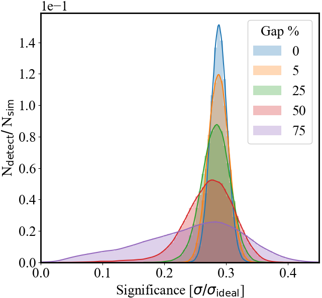
Figure 2: Probability density of the significances (relative to the significance of an ideal periodic signal) of the highest peak in the periodograms for different gap rates in the simulated LCs. The probability density distribution flattens and broadens significantly as the gap fraction is increased.

4.2 Gaps in a noise-dominated light curve

Figure 3: Probability density of the significances (relative to the maximum significance of a peak when no gap is present in the LC) of the highest peak in the periodograms for different gap rates in the random-noise LCs.

We simulate $N_{\mathrm{sim}}=10^{5}$ random white noise LCs along with random uncertainties for each data point on each LC as described in $\S$4.1. We also introduce gaps, just like in the case of the periodic LCs. Figure 3 shows the distribution of the relative significance of periods inferred from the random-noise LCs with different amounts of gaps; here, $\sigma_{\mathrm{0,max}}$ is defined as the maximum significance observed for a peak in the periodogram when the LCs have no gaps. The median of relative significance increases with increased gaps. The LC of PG 1553+113 has a gap of $17\%$ after binning, which increases the median of the relative significance by $\sim$12% compared to the LC without gaps. For 50% of gaps, the median of the relative significance is $\sim$50% larger. It is evident from the figure that gaps can increase the significance and produce significant false periodicities; however, the number, or the likelihood, of such false detections goes down with increased gaps.

Conversely, for $10^{6}$ randomly generated signals using the PG 1553+113-like PSD models explained in $\S$3.6, we find that the gaps in the LCs decrease the significance reported for the peak period. We find the median decrease is 2.2% for the $17\%$ gap case, and is 7.5% for the 50% gap using the PL model; for the BPL model, we instead find a decrease of 3.1% and a decrease of 10.4%, respectively.

Figure 4: Distribution of the peak frequencies with their corresponding significances (relative to the maximum significance) for a random-noise signal with 17% gap.

Figure 4 shows the observed frequency distribution and the corresponding relative significance distribution of the $N_{\mathrm{sim}}$ simulated random LCs, with a 17% gap. The vertical axis shows the significance of a peak frequency relative to the maximum significance of the distribution and the horizontal axis shows the frequency in the unit of per year. It is clear that a random noise signal does not generate any preferred period (see the constant distribution on top of Figure 4, and ignore the obvious edge effect). The same results are obtained for any amount of gaps. The difference in relative significance values is $\sim 3\%$, and the median frequencies varied by $\sim 2\%$ across all frequency bins. Therefore, the gaps are unlikely to produce a biased generation of a specific period.

We find similar results (relative significances and median frequencies vary by 5% and 1%) for PL and (by 3.5% and 1%) BPL using the specific PSD models for PG 1553+113 explained in $\S$3.6.

In conclusion, the gaps in random noise LCs affect the periodicity analysis, with a potential generation of significant false periodicity with gap rates far exceeding the 17% rate of PG 1553+113 (e.g. $\geq\,$50% of gaps). But this effect is not present when a periodic signal is real. Most importantly, the simulated LCs with the PG 1553+113-like PSD models do not show any effect of gaps in the significance. According to our tests, 17% of gaps in the optical LC of PG 1553+113 do not introduce any significant evidence that the observed period results from an artifact, nor does it affect the significance of said period.

5 Results

The PSD of the PG 1553+113 LC, and its PL and BPL fits from $\S$3.6, are shown in Figure 5.

Figure 5: PSD fits according to the PL and BPL estimates. The vertical dotted line shows the position of the peak period at 20.8 yr.

The outcome of the periodicity analysis is presented in Figures 6 and 7. The GLSP reveals a longer-term period of $20.8\pm 1.9$ years with a local significance (i.e. not corrected for trials) of $3.2\sigma$ for the PL and $2.7\sigma$ for the BPL.

The WWZ analysis indicates a period of $21.8\pm 4.7$ years, with a local significance of $2.7\sigma$ for the PL and $4.0\sigma$ for the BPL. This period is evident throughout the light curve (see Figure 7).

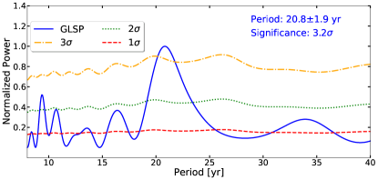
Figure 6: PG 1553+113 GLSP from the combined V-band LC. The highest peak is at 20.8$\pm$1.9 years. The significance is obtained with the PL model of $\S$3.6.

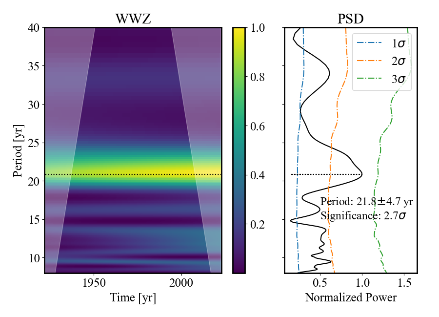
Figure 7: PG 1553+113 WWZ from the combined V-band LC. The color bar represents the normalized PSD, and the black dotted line shows the strongest period on both plots. A bright horizontal band covering the whole time scale suggests that the period of $21.8\pm 4.7$ years is stable and present in the whole LC. The white-shaded region in the wavelet plot shows the region outside the cone of influence where the edge effects become important. The significance is obtained with the PL model of $\S$3.6.

5.1 Trial correction

The significance obtained by the analysis methods has to be corrected for the look-elsewhere effect, resulting in the global significance of the period observed (Gross & Vitells, 2010). This global significance is approximated by

$$p_{\mathrm{global}}=1-(1-p_{\mathrm{local}})^{N},$$ (7)

where $N$ is simply the number of independent periods in each periodogram, because we only have one source (otherwise, the number of sources in the sample must also be counted Peñil et al., 2022). $N$ is estimated by performing Monte Carlo simulations. Specifically, we apply the algorithm described in Peñil et al. (2022), using $10^{8}$ simulated LCs with the technique of Timmer & Koenig (1995), obtaining the experimental relationship between local and global significance, then we determine $N$ by fitting Equation 7 to it. We fit specifically over the range $\geq 2\sigma$, since that is the range of local significance we obtained in our analysis. We consider an upper limit on $N$ of 100, since our periodograms include 100 periods; this balances between computational time and resolution in the periodograms. This procedure yields $N$=43, which according to Equation 7, maps a local significance of $\approx 3\sigma$ to a global significance of $\approx 1.9\sigma$.

5.2 False alarm probability

As an alternative measure of significance, we determine the false alarm probability. This is the probability that a PG 1553+113-like, pure-noise LC produces a peak period with a given local significance; we use 3$\sigma$ as a representative value of the local significances we found above in $\S$5. We generate $10^{6}$ LCs using both the PL and BPL noise models, and use the same sampling as the 28-day binned LC of PG 1553+113.

We find the false detection rate to be $\sim 4.9\%$ and $\sim 2.9\%$ for LCs generated using the PL and BPL noise models, respectively. These values of false detection rate are similar to the $p$-value one would obtain from the $\sim 2\sigma$ global significance we obtain in $\S$5.1.

The false alarm rate for the 2.2-year periodicity, as determined based on Peñil et al. (2023)’s findings, is $\sim 0.6\%$, indicating a low likelihood of spurious detection. If the 2.2- and 22-year periods are independent events, this implies that the false alarm probability for the simultaneous presence of both periods is roughly $\sim 0.02\%$.

5.3 Complementary study

We perform further analysis to investigate how the DASCH, MDB, and DASCH+MDB segments of the LC have on our detection of the periodic signal. As previously discussed, the DASCH data has some limitations, including gaps in the LC and larger uncertainties in the data points compared to the MDB data.

Individual periodicity analyses are carried out for each subset of the LC separately, using the GLSP and WWZ methods (using the PL method to find the local significance). The results of this analysis are presented in Table 1. The GLSP and WWZ analyses of the DASCH data report significances 22% and 15% below that of the complete LC (DASCH+MDB), respectively. The MDB data does not show any meaningful period of around 22 years, which is expected since the temporal baseline of the MDB data is shorter than this period. These results indicate that the slow oscillation we report in this study is not solely due to the MDB but that the DASCH data plays a vital role in detecting this longer-term period of PG 1553+113.

Table 1: Periodicity analysis on LC subsets.

	DASCH	MDB	DASCH+MDB
GLSP	$20.1\pm 3.9$ years ($\approx 2.5\sigma$)	No detection	$20.8\pm 1.9$ years ($\approx 3.2\sigma$)
WWZ	$25.0\pm 12.5$ years ($\approx 2.3\sigma$)	No detection	$21.8\pm 4.7$ years ($\approx 2.7\sigma$)

Combining the new observations with the archived optical LC not only strengthens the power of the $\sim 22$-yr peak, but also increases its significance by $\sim 17\%-28\%$ and reduces the uncertainty by $\sim 60\%$.

In Figure 8, we phase-folded the LC to highlight the oscillation, using the 21.8-year period obtained from the WWZ method. We also smoothed the MDB data using the savgol filter, which removes the scatter from the 2.2-year periodicity and reveals that the MDB LC closely follows the $\sim$22-year oscillation.

Figure 8: Phase folded plot with binned DASCH and MDB data. The smoothed MDB follows the 21.8 yr sinusoidal fit.

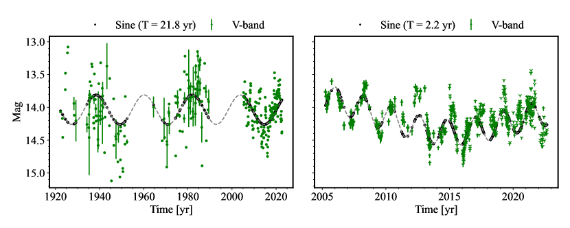
Figure 9: Sinusoidal reconstruction according to the two periods detected from the optical emission of PG 1553+113. Left: a fit of the entire optical LC with a $\sim 22$-yr period. Right: a fit of the MDB optical LC with a $\sim 2.2$-yr period. The $\sim 22$-yr fit is superposed, which explains the trends discussed in $\S$1.

Figure 10: Sinusoidal fit from Figure 9 (Right) is extended further to predict the fast oscillation extrema. The next maxima in optical emission is predicted around June 2023, and the next minima in July 2024.

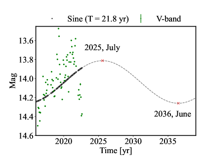
Figure 11: Sinusoidal fit from Figure 9 (Left) is extended further to predict the slow oscillation extrema. The next maxima in optical emission is predicted around July 2025, and the next minima in June 2036.

We present two sinusoidal reconstructions of the optical emission of PG 1553+113, one using the period of 21.8 years obtained from our analysis and the other using 2.2 years from the literature. These reconstructions are shown in Figure 9. For the fast oscillation of 2.2 years, the most recent high-emission state is predicted to occur in June 2023, followed by a low in July 2024 (see Figure 10). For this fast oscillation, no known delay between the optical and $\gamma$-ray emission exists (both emissions are correlated, see Peñil et al., 2023). Therefore, we expect the maxima/minima of $\gamma$-ray emission to co-occur with optical. For the slow oscillation of approximately 22 years (Figure 11), the next high-emission state is expected to occur in July 2025, followed by a low in June 2036. However, in Peñil et al. (2023), a delay of at least roughly two years between the optical and $\gamma$-ray emission is tentatively noticed, and if real, would lead to the next high-emission state in $\gamma$-rays (associated with the slow oscillation) in July 2023 and a low in June 2034. In the absence of any lag, the $\gamma$-ray emission will occur concurrently with the optical counterpart. We show a cartoon representing the double periodicity observed in the LC of PG 1553+113 (seen in Figure 9) in Figure 12. The figure illustrates the long-term period plus a trend, discussed in $\S$1, as part of a longer-term period that we have labeled the “lump period” (see $\S$6 for a discussion of the lump period).

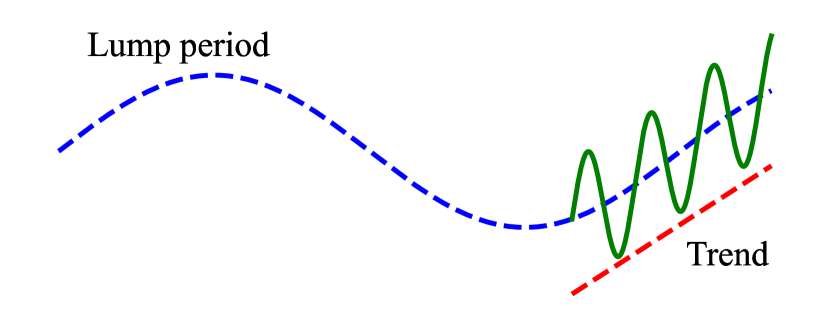
Figure 12: A trend in a PG 1553+113 LC, discussed in $\S$1, is indicated in this illustration by the red dashed line. The fast and slow oscillations reflect the orbital and the lump periods, respectively, from our binary SMBH interpretation of the source (see $\S$6). Here, the trend is shown as a rising segment of the lump period.

We are not able to detect the presence of the short period of 2.2 years in the DASCH data. This is due to the average number of observations in the archival data being 2.1 per year, compared to 8.2 per year in the MDB data. The limited number of observations and uneven sampling in the DASCH data make detecting such a short period challenging. The archival data, on average, just barely meets the theoretical sampling rate of 4 points per cycle (Landau, 1967), but to determine the frequency and amplitude of a signal, the sampling needs to be in phase with the signal. The observations in the DASCH data fail to meet this requirement.

6 Discussion & theoretical interpretation

In this section, we assume a fiducial total black hole mass for PG 1553+113 (hereafter just “PG 1553”) of $M=5\times 10^{8}\,M_{\odot}$, where $M_{\odot}$ denotes a solar mass, and a binary semi-major axis $a=5\times 10^{-3}\,$pc, which imply a binary orbital period $T_{\rm binary}=1.5\,$yrs in the source frame. This orbital period corresponds to the observed $2.2$-yr periodicity when a redshift of $\sim 0.433$ is assumed (Danforth et al., 2010; Johnson et al., 2019; Dorigo Jones et al., 2021). A Newtonian treatment of the disk should suffice at distances $\simeq\mathcal{O}(a)$ from the black holes since the characteristic gravitational length scale $L=GM/c^{2}$ is much smaller than $a$, i.e. $L/a\simeq 5\times 10^{-3}$, where $G$ is Newton’s gravitational constant and $c$ is the speed of light. This binary is likely in the gravitational wave-driven regime of orbital evolution (Peñil et al., 2023), and over the last 100 years, gravitational wave decay is on the order of $0.01\times T_{\rm binary}$ (Peters, 1964), which is negligible compared to our uncertainties. Our assumed mass is consistent with the estimate of $(0.4-8)\times 10^{8}M_{\odot}$, based on light curve variability (Dhiman et al., 2021), and is typical of masses in existing binary models of PG 1553 (Cavaliere et al., 2017; Tavani et al., 2018; Huang et al., 2021). See also Ackermann et al. (2015) for a rough estimate of $1.6\times 10^{8}M_{\odot}$ based on the empirical relationship between blazar jet power and disk luminosity presented in Ghisellini et al. (2014). We adopt standard geometrically thin, optically thick, constant-$\alpha$ disk models (Shakura & Sunyaev, 1973; Goodman, 2003), with a monatomic adiabatic equation of state (adiabatic index $\Gamma=5/3$), a radiative efficiency $\eta=10\%$, and an opacity dominated by electron scattering. We use a physical radiative cooling prescription, and we relate the disk effective temperature $T_{\rm eff}$ to the midplane temperature $T$, surface density $\Sigma$, and opacity $\kappa$, via $T_{\rm eff}^{4}=(4/3)\,T^{4}/(\kappa\Sigma)$ (Frank et al., 2002).

We perform two-dimensional viscous hydrodynamic simulations of binary accretion with an Eulerian grid-based code Sailfish (for details, see Westernacher-Schneider et al., 2022). Radiation pressure is omitted in simulations due to its technical difficulty. Instead, the characteristic aspect ratio $h$ of the disk is chosen to be similar to a disk whose radiation and gas pressures are accounted for. The aspect ratio is defined as $h=H/r$, where $H$ is the disk half-thickness. We consider a fiducial accretion rate of $0.1M_{\rm Edd}$ typical of blazars Ghisellini et al. (2014), which yields characteristic disk aspect ratios $h\in\{0.015,0.03,0.045\}$ when measured around an equilibrium circumsingle disk at radii $r\in\{a,a/2,a/3\}$, respectively. Note that an accretion rate of $0.1M_{\rm Edd}$ is consistent with PG 1553’s putative binary being in the gravitational wave-driven regime (Peñil et al., 2022); below we describe the implications of this for the binary’s eccentricity.

6.1 Implications for the binary hypothesis

Accreting binaries are known to hollow out a cavity and generate an $m=1$ overdensity in the circumbinary disk (MacFadyen & Milosavljević, 2008), called a “lump,” for certain regions of parameter space (D’Orazio et al., 2013; Miranda et al., 2017; Duffell et al., 2020; Zrake et al., 2021), including disks initialized with a large misalignment relative to the orbital plane of the binary (Moody et al., 2019). The periodicity associated with the lump depends on the cavity size, and in Westernacher-Schneider et al. (2022) a lump period range of $4.5-10.8$ binary orbits is reported based on a large suite of radiatively cooled, adiabatic two-dimensional disk models around circular, equal-mass binaries. In that work, the lump period was found to depend most strongly on the disk’s aspect ratio $h$; thinner disks exhibit longer lump periods. This range of lump periods accommodates most values reported so far in the literature, with some exceptions extending as low as $\sim 3.6$ binary orbits (Bowen et al., 2019). Hence, in this work, we consider our a priori possible range of lump periods to be $3.6-10.8$ binary orbits.

Assuming PG 1553’s $2.2$-yr periodicity corresponds to the binary orbit, its $10\times$ longer period of $22$ yrs is consistent with the high end of this theoretical lump period range. The high end is mostly populated by two-dimensional models of adiabatic, radiatively cooled disks that are sufficiently thin ($h\lesssim 0.09$, see, e.g. Farris et al., 2015; Westernacher-Schneider et al., 2022). Assuming a standard value for the dimensionless viscosity parameter of $\alpha=0.1$, PG 1553’s disk aspect ratio satisfies this thinness condition on radial distances $r\sim\mathcal{O}(a)$ for accretion rates below $\sim 0.6\times$ the Eddington rate. BL Lac objects like PG 1553 are safely below such accretion rates (see e.g. Paliya et al., 2021). Thus, the 10:1 period ratio exhibited in its optical light curve might be explained by a binary engine.

In binary accretion models that assume isothermal gas, lumps register in total black hole accretion rates when the binary has mass ratio $q\gtrsim 0.2$ and eccentricity $e\lesssim 0.1$ (D’Orazio et al., 2013; Miranda et al., 2017; Muñoz et al., 2020; Duffell et al., 2020; Zrake et al., 2021). The same models predict that, in the gas-driven regime of orbital evolution, binaries accreting from prograde disks have an attractor value of eccentricity of a few tens of percent, with a wide basin of attraction (e.g. Roedig et al., 2011; Roedig & Sesana, 2014; Zrake et al., 2021; D’Orazio & Duffell, 2021; Siwek et al., 2023). One might therefore expect most binaries to have significant eccentricity upon entering the gravitational wave-driven regime, at which time the binary begins to circularize. On its face, since PG 1553’s putative binary seems safely in the gravitational wave-driven regime, it is plausible that its eccentricity is now small enough ($e\lesssim 0.1$) to generate a significant lump in its circumbinary disk. If PG 1553 hosts a binary and a lump, then these constraints ($e\lesssim 0.1$, $q\gtrsim 0.2$) can be applied to PG 1553’s putative binary. In Section 6.3, we apply these constraints to some binary models proposed in the literature.

6.2 How the lump can imprint on jet emission

Since PG 1553 is a very high energy ($E>100\,$GeV) BL Lac blazar, its emission is overwhelmed by its jet(s). Thus, we must consider mechanisms by which lump periodicity could transmit to jet power. We consider two mechanisms, lump-modulation of the accretion rate onto the jet-launching black hole(s) (hereafter the “accretion rate mechanism”), and lump-modulation of the supply of seed photons from the circumbinary disk (hereafter the “seed photon mechanism”). The accretion rate in the disk is a systemic parameter in theoretical jet-launching mechanisms (Blandford & Znajek, 1977; Blandford & Payne, 1982), and observational evidence exists for a correlation between jet power and accretion (e.g. Ghisellini et al., 2014). Therefore, one expects that accretion rate modulations imprint upon all components of jet spectral energy distributions (SEDs), so long as such modulations take place on time scales much longer than black hole dynamical times (so that jet power can adjust quasi-statically). This includes imprints on the synchrotron component, which dominates the optical band in two-component models of PG 1553’s SED (see, e.g. Osterman et al., 2006; Albert et al., 2007; Aleksić et al., 2012; Raiteri et al., 2015, 2017).

On the other hand, thermal seed photons from the disk at a radius $\simeq 4.7\,a$ (presumed to be the characteristic lump location, yielding a lump orbital period of $\simeq 10$ binary orbits) peak in the range of mid-infrared to optical bands for a large range of accretion rates, i.e. between $0.01-1\times$ the Eddington rate. Such photons, upscattered by electrons with fiducial blazar jet Lorentz factors $\gamma\simeq 10$ (Ghisellini et al., 2014), would reach at least soft X-ray energies. These are similar energetics of the external Compton process considered in Band & Grindlay (1986) (e.g. optical seed photons upscattering to X-rays). Thus, since the $\sim 22$-year period is detected in the optical band, the lump model of this modulation indicates that the accretion rate mechanism must be operative.

Even if a lump is present, how strongly lump periodicity transmits to black hole accretion rates can depend on model details, including physical parameters like the size of the black hole in relation to its minidisk (e.g. compare Farris et al., 2015; Westernacher-Schneider et al., 2022). Observations of lump periodicity at energies in the synchrotron bump could therefore shed light on details of the accretion physics.

While the presence of lump periodicity in optical emission implies that the accretion rate mechanism is operative, a comparison between optical and $\gamma$-ray bands shows tentative evidence that the seed photon mechanism is also operative. In the optical band, the most recent minimum of the $\sim 22$-yr period occurs around 2016. However, in the more limited temporal baseline of $\gamma$-ray observations from 2009 until now, although a rising trend is apparent, no obvious minimum occurs around 2016 Peñil et al. (2023), although it is difficult to be sure without a longer temporal baseline. It appears as though lump periodicity in optical emission instead lags $\gamma$-rays by several years. Radio emission appears to share the same lag as $\gamma$-rays Peñil et al. (2023). These lags might be accounted for in the lump model if the seed photon mechanism contributes significantly to $\gamma$-ray emission. Simulations predict that lump-modulated black hole accretion rates can lag lump-modulated thermal disk emission by $\approx 20-30\%$ of a lump period (see Figure 5 in Farris et al., 2015). Thus, since $\gamma$-rays can receive imprints via both the accretion rate and seed photon mechanisms, whereas optical emission only receives an imprint via the accretion rate mechanism, it is possible that lump-induced minima in optical emission lag those in $\gamma$-ray emission. Continued monitoring of PG 1553 for many years is therefore crucially important for making an accurate determination of the relative phase of the $\sim 22$-yr modulation between low- and high-energy bands.

It is important to note that the SED of PG 1553 is usually modeled using only synchrotron and synchrotron self-Compton components (SSC models, see e.g. Osterman et al., 2006; Albert et al., 2007; Aleksić et al., 2012; Raiteri et al., 2015, 2017), and likewise for BL Lac objects generally (but it has been cautioned that this may not always be justified, see e.g. Ghisellini & Madau, 1996). The adequacy of SSC fits of SEDs suggests that seed photons from the disk are negligible. However, since PG 1553 has a compton dominance of $\sim 1$, a non-negligible contribution of external Compton emission may be present in its SED. Thus, a three-component SED model (SSC+EC) with a significant disk-driven external Compton component (which the multiwavelength data and binary hypothesis tentatively require) must appear degenerate with current SSC models to within uncertainties. Therefore, in future work it is well-motivated to carefully evaluate SSC+EC models of PG 1553.

6.3 Implications for existing binary models

Figure 13: Simulations of accretion onto a circular binary with mass ratio $q=0.4$, total black hole mass $M=5\times 10^{8}M_{\odot}$, and orbital period of 1.5 yrs in the source frame. Three characteristic disk aspect ratios are shown, $h\in\{0.015,0.03,0.045\}$. The left panels show snapshots of the disk surface density, raised to the $1/4$th power to improve visual contrast. Black holes are indicated with white dots and are orbiting counter-clockwise. Thinner disks have larger cavities and correspondingly longer lump periods. A 10:1 relationship between lump and binary orbital periods is bracketed by these models (see the rightmost panel), consistent with the 2.2-yr and 22-yr periods detected in PG 1553 light curves.

Cavaliere et al. (2017) and Tavani et al. (2018) propose a binary model of PG 1553’s $2.2$-year periodicity based on periodic driving of magnetohydrodynamic instabilities in the jet(s) due to the gravitational influence of the binary. The stipulated binary mass ratio is $q=0.1$, and a binary eccentricity of $e\sim 0.2$ is obtained by fitting the model to PG 1553 light curves. Both of these parameters are outside the aforementioned lump-producing range suggested by isothermal binary accretion models. The model proposed in Cavaliere et al. (2017) and Tavani et al. (2018) is therefore disfavored. It remains to be seen whether the binary parameters of this model can be adjusted into the lump-producing range while still producing an adequate fit of the $\sim 2.2$-yr periodicity.

Another recent binary model of PG 1553’s $2.2$-year periodicity, based on a two-jet precession scenario, arrives at $q\sim 0.4$ and assumes $e=0$ (Huang et al., 2021). These parameters fall into the aforementioned lump-producing range, and the mass ratio is consistent with one of the lower bounds ($q>0.35$) proposed by Caproni et al. (2017) based on jet precession scenarios. To assess whether this model can produce a 10:1 lump-to-binary period ratio, we ran $q=0.4$, $e=0$ binary accretion simulations with characteristic disk aspect ratios $h\in\{0.015,0.03,0.045\}$ (see our basic assumptions at the beginning of §6). These disk aspect ratios are consistent with the lower bound $h>0.0027-0.0048$ proposed in Caproni et al. (2017) based on jet precession models of the $\sim 2.2$-yr periodicity. We ran for 4000 binary orbits at a resolution of $\Delta x=0.016\,a$, corresponding to $1-10$ viscous times $(2/3)a^{2}/\nu$, then refined the grid to $\Delta x=0.008\,a$ and ran for 420 more binary orbits. The analysis is performed over the latter 320 binary orbits. To quantify the lump period, we compute the PSD of the phase of the circumbinary disk’s $m=1$ density moment (which we call the “lump PSD”). The $m=1$ moment is computed over $1.5\,a<r<12\,a$, and long-term trends due to cavity precession are subtracted before computing the PSD. Our simulation results are shown in Figure 13. The first three panels show $\Sigma^{1/4}$ snapshots for the three characteristic aspect ratios we consider, and the last panel shows the corresponding lump PSDs normalized to the lump peak. Differing cavity sizes are apparent in the snapshots, and the last panel shows that a 10:1 lump-to-binary period ratio is bracketed by these models (see the shaded interval). The binary parameters proposed in Huang et al. (2021) therefore appear consistent with a lump model of PG 1553’s $22$-yr periodicity.

6.4 Could the $22$-year period be a minidisk evaporation cycle?

Each black hole in an accreting binary has its own “minidisk,” while the whole binary is surrounded by a circumbinary disk. Recent numerical work, which includes radiation pressure from the inner disks around binary black holes, tentatively suggests that black hole minidisks can undergo cycles of formation and destruction on a time scale of $6-18$ binary orbits (Williamson et al., 2022). In this process, as minidisks form, accretion onto the black holes ramps up, generating radiation pressure that eventually reaches a level that evaporates the minidisks. Once the minidisks evaporate, radiation pressure shuts off, allowing the minidisks to form again by feeding from the circumbinary disk.

A similar duty cycle of partial evaporation could conceivably cause accretion rate modulation on a time scale of 10 binary orbits. However, Williamson et al. (2022) did not rule out the possibility that their proposed duty cycle is an artifact of manually and abruptly turning radiation pressure on and off. Furthermore, their setup assumed optically thin gas, appropriate for binaries with sufficiently wide separation. The gas at radii $r\sim a$ in PG 1553 should be highly ionized, and thus optically thick to electron scattering (Haiman et al., 2009). Optical thickness would inhibit the ability of a central radiation source to evaporate the minidisks. Further theoretical work is therefore required to establish whether this process is realistic for a putative binary in a PG 1553-like system.

6.5 Mechanism for PG 1553’s $\sim 2.2$-year periodicity

Stochastic flaring is an increasingly unlikely explanation of PG 1553’s $2.2$-yr periodicity, since 7 or more putative periods are measured, depending on the energy band, and the statistical significance seems to be increasing over time (see, e.g. Peñil et al., 2022, 2023). The additional detection of a $22$-yr periodicity, consistent with a lump, further increases the chances that the $2.2$-yr periodicity is genuine. Two binary models of PG 1553’s $2.2$-yr periodicity proposed in the literature are jet precession (Caproni et al., 2017; Huang et al., 2021) and gravitationally induced magnetohydrodynamic instabilities in the jet(s) Cavaliere et al. (2017); Tavani et al. (2018). Since PG 1553’s disk mass is expected to be negligible compared to the black hole mass, both of these mechanisms, both stemming from black hole masses and spins, are unlikely to be affected by the presence of a lump. However, accretion rate variability on the binary’s orbital time scale might explain the $2.2$-yr periodicity, or will at least coexist with the aforementioned mechanisms. In this section, we enumerate accretion rate variability mechanisms that could explain PG 1553’s $2.2$-yr periodicity, focusing on the time scales involved, and we judge their viability.

1. Accretion variability at (or near) $f_{\rm binary}$: as is well-known (e.g. see the recent review in Lai & Muñoz, 2022), accretion rates are generally variable on the binary orbital time scale. In fact, such orbital peaks are usually found to be absent in only limited ranges of binary parameters, such as small mass ratios (i.e. too small to form a lump), or towards the idealized circular, equal-mass case (see, e.g. MacFadyen & Milosavljević, 2008; Shi et al., 2012; Noble et al., 2012; Farris et al., 2014; Muñoz et al., 2020; Duffell et al., 2020).

   However, even for the circular, equal-mass case, it was recently found (Westernacher-Schneider et al., 2022, 2023) that the minidisks can develop significant eccentricity, causing them to trade mass at a near-orbital beat frequency $f_{\rm binary}-f_{\rm prec}$ between the binary and the eccentric minidisk precession rate $f_{\rm prec}$. The generality of accretion variability at (or near) $f_{\rm binary}$, therefore, makes it a plausible candidate mechanism to generate the $2.2$-yr periodicity.

   In addition, for mass ratios near $q\sim 0.4$, accretion rate variability at the lump and orbital periods were found to be comparable in recent work (e.g. Duffell et al., 2020; Muñoz et al., 2020). This suggests it is realistic to expect the observed similar amplitudes of the $2.2$-yr and $22$-yr periodicities in the PG 1553 optical light curve, but more realistic models are required to be sure.

2. Accretion variability at $\sim(1.4-2)f_{\rm binary}$: two recent studies report mass transfer variability between minidisks, dubbed “minidisk sloshing” (Bowen et al., 2017; Avara et al., 2023); the most recent study reports variability at a dominant frequency of $1.4f_{\rm binary}$. This effect was found to occur for sufficiently relativistic gravitational potentials (binary semi-major axis $a\lesssim 150GM/c^{2}$), leading to associated black hole accretion rate variability. Since the putative binary in PG 1553 has $a\sim 200GM/c^{2}$, this is unlikely to be the mechanism of the $2.2$-yr periodicity. If it were, then the $2.2$-yr period is less than a binary orbit, meaning the binary is even more widely separated (i.e. less relativistic), further reducing the odds that the minidisk sloshing mechanism is operative.

   Accretion variability at $2f_{\rm binary}$ into the central cavity is also found for nearly circular, nearly equal-mass binaries (e.g. MacFadyen & Milosavljević, 2008; Farris et al., 2014; Miranda et al., 2017), likely due to the binary stripping material from the near-side of the cavity wall twice per orbit. However, such variability is generally found to be quite suppressed when measured at the black hole locations (e.g. Farris et al., 2014; Muñoz et al., 2020; Duffell et al., 2020), and therefore would not transmit significantly to a jet’s base.

3. Accretion variability at $2(f_{\rm binary}-f_{\rm lump})$ (e.g. Roedig et al., 2012; Noble et al., 2012; Shi et al., 2012; Shi & Krolik, 2015): for circular, equal-mass binaries with cavities that are sufficiently circular and close to the binary (see exceptions in Farris et al., 2015; Westernacher-Schneider et al., 2022, 2023), variability was reported at a beat frequency between the binary and the lump, $2(f_{\rm binary}-f_{\rm lump})$. A 10:1 ratio between this frequency and $f_{\rm lump}$ is obtained if $T_{\rm lump}=6\,T_{\rm bin}$, which is a theoretically reasonable lump period. While this is a possible mechanism to explain the $2.2$-yr variability, this operates in a narrow region of parameter space (i.e. $e\sim 0$, $q\sim 1$, and small cavities), and thus is less general than e.g. accretion variability at $f_{\rm binary}$.

6.6 Multiple periods from a single black hole

It is known that electromagnetic emission from the vicinity of a single, accreting, spinning black hole can exhibit multiple QPOs simultaneously (see Ingram & Motta, 2019, for a recent review), although observing any QPOs at all from active galactic nuclei has been more difficult than from stellar-mass black holes (Vaughan & Uttley, 2005). These QPOs could arise from precessional phenomena driven by torques applied to the surrounding gas by the spinning black hole. For example, the relativistic precession model (RPM, see, e.g. Stella & Vietri, 1998; Stella et al., 1999) predicts three hierarchical precessional frequencies for a particle in a geodesic orbit slightly off a compact object’s equatorial plane. All three frequencies may be observed in rare cases (e.g. Motta et al., 2014). More disk-like pictures involve the Bardeen-Petterson effect (Bardeen & Petterson, 1975), and for sufficiently large tilt angles between the disk and the black hole spin, the disk can “break” into two (e.g. Lodato & Price, 2010) or more annuli that precess independently (Liska et al., 2021). Such precession can steer a jet (Liska et al., 2018), thereby imprinting periodic line-of-sight variation onto emission. In forthcoming work, we will present a detailed assessment of the single black hole precessional hypothesis for PG 1553’s multiple periods.

6.7 Characterization of gravitational wave signal and the merger time

A binary SMBH system emits a gravitational wave (GW) signal until it coalesces (Begelman et al., 1980). We characterize the continuous GW frequency and strain amplitude emitted from PG 1553’s putative binary central engine. The GW frequency is dominated by twice the orbital frequency, which corresponds to the continuous GW frequency of $\sim 4\times 10^{-8}$ Hz given the $1.5$-yr binary orbital period ($\sim 2.8\times 10^{-8}$ Hz in the observer frame, assuming a redshift $z=0.433$). Using the methods described by Buskirk & Hamilton (2019) and the implementation by van Zeist et al. (2021), we estimate the strain amplitude to be $\sim 10^{-17}$. In this estimate, we used a mass ratio of $q=0.4$, following Huang et al. (2021). Our estimates of GW strain amplitude and frequency are similar to those reported in Cavaliere et al. (2019).

PG 1553’s GW frequency is in the detectable range for pulsar timing arrays, but the strain is two orders of magnitude lower than the current sensitivity limit of NANOGrav (see Figure 8c of Agazie et al., 2023). Even with 20 years of observation, PG 1553’s GW strain is expected to be $\sim 10\times$ lower than the sensitivity of the Square Kilometer Array pulsar timing array (Moore et al., 2014).

The time to merger for a binary black hole system is given by $T_{\rm merge}=a^{4}/4\beta$ (Peters, 1964). Here $a$ is the semi-major axis and $\beta$ is defined as,

$$\beta=\frac{64}{5}\frac{G^{3}}{c^{5}}m_{1}m_{2}(m_{1}+m_{2}),$$ (8)

where $m_{1}=3.57\times 10^{8}\,M_{\odot}$ and $m_{2}=1.43\times 10^{8}\,M_{\odot}$ are the masses of two SMBHs. The merger time formula assumes a circular orbit, and gas-driving effects, while subdominant in the GW-dominated regime, are neglected completely in this merger time estimate. We find the $T_{\rm merge}\sim 15000$ years for the PG 1553+113 system. The estimation of merger time is sensitive to the total mass of the system; for the extremes of the total mass estimates $(0.4-8)\times 10^{8}\,M_{\odot}$ (Dhiman et al., 2021), the merger times range from $7000-10^{6}$ years.

7 Summary

In conclusion, our analysis of the $\sim$100-year V-band optical LC of PG 1553+113 revealed a significant multi-decade period of $\sim$22 years, which by itself has 1.9$\sigma$ significance after accounting for the look-elsewhere effect. A simple estimate of the chance of noise producing both this oscillation and the known $\sim$2.2-year oscillation, assuming they are independent occurrences, is $\sim 0.02\%$ (3.5$\sigma$). We perform an intense program of tests, including measuring the impact of gaps in the data and the impact of the DASCH data alone versus the MDB data alone on the evidence for the $\sim$22-year period. We conclude it is unlikely that the slow oscillation period is an artifact of such factors. We suggest an interpretation of the longer-term oscillation in which an $m=1$ mode (the so-called “lump”) has formed in the accretion disk around a binary SMBH and modulates the rate of mass delivery to the binary on a 22-year cycle, ultimately leading to a corresponding modulation of jet power. This interpretation is supported by our targeted modeling simulations, which show that a 10:1 ratio between the binary orbital period and the lump period can be obtained with plausible binary accretion parameters for PG 1553+113.

Based on our findings, we predict that the peak of the emission associated with this period will likely be observed in July 2025. These results contribute to our understanding of PG 1553+113 as a binary SMBH candidate.

Additionally, we found the continuous GW signal from PG 1553+113’s putative binary engine has a strain amplitude well below the detection threshold of foreseeable pulsar timing arrays.

To better understand periodicity in binary blazar emission, future theoretical work should constrain the relative importance of various mechanisms, such as the aforementioned accretion rate and seed photon mechanisms (e.g., Peñil et al., 2023), jet precession (e.g., Huang et al., 2021), and gravitationally induced magnetohydrodynamic instabilities (e.g., Cavaliere et al., 2017). A greater understanding of these processes may teach us more about the binary scenario, and jet physics generally, using information we did not evaluate in detail, such as the relative amplitude of the $2.2$-yr and $22$-yr signals, and multiwavelength data.

8 Acknowledgments

We want to thank all the observatories from which we used data. The DASCH project at Harvard is grateful for partial support from NSF grants AST-0407380, AST-0909073, and AST-1313370. We thank the Las Cumbres Observatory and its staff for their continuing support of the ASAS-SN project. ASAS-SN is supported by the Gordon and Betty Moore Foundation through grant GBMF5490 to the Ohio State University and NSF grants AST-1515927 and AST-1908570. Development of ASAS-SN has been supported by NSF grant AST-0908816, the Mt. Cuba Astronomical Foundation, the Center for Cosmology and Astroparticle Physics at the Ohio State University, the Chinese Academy of Sciences South America Center for Astronomy (CAS-SACA), the Villum Foundation, and George Skestos. The AAVSO database: Kafka, S., 2021, Observations from the AAVSO International Database, https://www.aavso.org. The CSS survey is funded by the National Aeronautics and Space Administration under Grant No. NNG05GF22G issued through the Science Mission Directorate Near-Earth Objects Observations Program. The Catalina Real-Time Transient Survey is supported by the U.S. National Science Foundation under grants AST-0909182 and AST-1313422. Based on observations obtained with the Samuel Oschin Telescope 48-inch and the 60-inch Telescope at the Palomar Observatory as part of the Zwicky Transient Facility project. ZTF is supported by the National Science Foundation under Grant No. AST-2034437 and a collaboration including Caltech, IPAC, the Weizmann Institute for Science, the Oskar Klein Center at Stockholm University, the University of Maryland, Deutsches Elektronen-Synchrotron and Humboldt University, the TANGO Consortium of Taiwan, the University of Wisconsin at Milwaukee, Trinity College Dublin, Lawrence Livermore National Laboratories, and IN2P3, France. Operations are conducted by COO, IPAC, and UW.

P.P. and M.A. acknowledge funding under NASA contract 80NSSC20K1562.

S.B. acknowledges financial support by the European Research Council for the ERC Starting grant MessMapp, under contract no. 949555.

A.D. is thankful for the support of the Ramón y Cajal program from the Spanish MINECO, Proyecto PID2021-126536OA-I00 funded by MCIN / AEI / 10.13039/501100011033, and Proyecto PR44/21‐29915 funded by the Santander Bank and Universidad Complutense de Madrid.

A.R. acknowledges the support of an Investigo grant funded by the European Union, Next Generation EU.

References

- Ackermann et al. (2015) Ackermann, M., Ajello, M., Albert, A., et al. 2015, ApJ, 813, L41
- Agarwal et al. (2021) Agarwal, A., Mihov, B., Andruchow, I., et al. 2021, A&A, 645, A137
- Agazie et al. (2023) Agazie, G., Anumarlapudi, A., Archibald, A. M., et al. 2023, ApJ, 951, L10
- Albert et al. (2007) Albert, J., Aliu, E., Anderhub, H., et al. 2007, ApJ, 654, L119
- Aleksić et al. (2012) Aleksić, J., Alvarez, E. A., Antonelli, L. A., et al. 2012, ApJ, 748, 46
- Astropy Collaboration et al. (2013) Astropy Collaboration, Robitaille, T. P., Tollerud, E. J., et al. 2013, A&A, 558, A33
- Astropy Collaboration et al. (2018) Astropy Collaboration, Price-Whelan, A. M., Sipőcz, B. M., et al. 2018, AJ, 156, 123
- Avara et al. (2023) Avara, M. J., Krolik, J. H., Campanelli, M., et al. 2023, arXiv e-prints, arXiv:2305.18538
- Band & Grindlay (1986) Band, D. L. & Grindlay, J. E. 1986, ApJ, 311, 595
- Bardeen & Petterson (1975) Bardeen, J. M. & Petterson, J. A. 1975, ApJ, 195, L65
- Begelman et al. (1980) Begelman, M. C., Blandford, R. D., & Rees, M. J. 1980, Nature, 287, 307
- Blandford & Payne (1982) Blandford, R. D. & Payne, D. G. 1982, MNRAS, 199, 883
- Blandford & Znajek (1977) Blandford, R. D. & Znajek, R. L. 1977, MNRAS, 179, 433
- Bowen et al. (2017) Bowen, D. B., Campanelli, M., Krolik, J. H., Mewes, V., & Noble, S. C. 2017, ApJ, 838, 42
- Bowen et al. (2019) Bowen, D. B., Mewes, V., Noble, S. C., et al. 2019, ApJ, 879, 76
- Buskirk & Hamilton (2019) Buskirk, D. & Hamilton, M. C. B. 2019, European Journal of Physics, 40, 025603
- Caproni et al. (2017) Caproni, A., Abraham, Z., Motter, J. C., & Monteiro, H. 2017, ApJ, 851, L39
- Cavaliere et al. (2019) Cavaliere, A., Tavani, M., Munar-Adrover, P., & Argan, A. 2019, ApJ, 875, L22
- Cavaliere et al. (2017) Cavaliere, A., Tavani, M., & Vittorini, V. 2017, ApJ, 836, 220
- Chakraborty & Rieger (2020) Chakraborty, N. & Rieger, F. M. 2020, arXiv e-prints, arXiv:2010.01038
- Connolly (2015) Connolly, S. D. 2015, arXiv e-prints, arXiv:1503.06676
- Danforth et al. (2010) Danforth, C. W., Keeney, B. A., Stocke, J. T., Shull, J. M., & Yao, Y. 2010, ApJ, 720, 976
- Dey et al. (2018) Dey, L., Valtonen, M. J., Gopakumar, A., et al. 2018, ApJ, 866, 11
- Dhiman et al. (2021) Dhiman, V., Gupta, A. C., Gaur, H., & Wiita, P. J. 2021, MNRAS, 506, 1198
- D’Orazio & Duffell (2021) D’Orazio, D. J. & Duffell, P. C. 2021, ApJ, 914, L21
- D’Orazio et al. (2013) D’Orazio, D. J., Haiman, Z., & MacFadyen, A. 2013, MNRAS, 436, 2997
- Dorigo Jones et al. (2021) Dorigo Jones, J., Johnson, S. D., Muzahid, S., et al. 2021, in American Astronomical Society Meeting Abstracts, Vol. 53, American Astronomical Society Meeting Abstracts, 116.02
- Drake et al. (2009) Drake, A. J., Djorgovski, S. G., Mahabal, A., et al. 2009, ApJ, 696, 870
- Drake et al. (2013) Drake, A. J., Catelan, M., Djorgovski, S. G., et al. 2013, ApJ, 763, 32
- Duffell et al. (2020) Duffell, P. C., D’Orazio, D., Derdzinski, A., et al. 2020, ApJ, 901, 25
- Emmanoulopoulos et al. (2013) Emmanoulopoulos, D., McHardy, I. M., & Papadakis, I. E. 2013, MNRAS, 433, 907
- Farris et al. (2014) Farris, B. D., Duffell, P., MacFadyen, A. I., & Haiman, Z. 2014, ApJ, 783, 134
- Farris et al. (2015) Farris, B. D., Duffell, P., MacFadyen, A. I., & Haiman, Z. 2015, MNRAS, 446, L36
- Foreman-Mackey et al. (2013a) Foreman-Mackey, D., Hogg, D. W., Lang, D., & Goodman, J. 2013a, PASP, 125, 306
- Foreman-Mackey et al. (2013b) Foreman-Mackey, D., Hogg, D. W., Lang, D., & Goodman, J. 2013b, PASP, 125, 306
- Foster (1996) Foster, G. 1996, AJ, 112, 1709
- Frank et al. (2002) Frank, J., King, A., & Raine, D. J. 2002, Accretion Power in Astrophysics: Third Edition (Cambridge University Press)
- Ghisellini & Madau (1996) Ghisellini, G. & Madau, P. 1996, MNRAS, 280, 67
- Ghisellini et al. (2014) Ghisellini, G., Tavecchio, F., Maraschi, L., Celotti, A., & Sbarrato, T. 2014, Nature, 515, 376
- Goodman (2003) Goodman, J. 2003, MNRAS, 339, 937
- Goyal et al. (2017) Goyal, A., Stawarz, Ł., Ostrowski, M., et al. 2017, ApJ, 837, 127
- Grindlay et al. (2009) Grindlay, J., Tang, S., Simcoe, R., et al. 2009, in Astronomical Society of the Pacific Conference Series, Vol. 410, Preserving Astronomy’s Photographic Legacy: Current State and the Future of North American Astronomical Plates, ed. W. Osborn & L. Robbins, 101
- Gross & Vitells (2010) Gross, E. & Vitells, O. 2010, European Physical Journal C, 70, 525
- Haiman et al. (2009) Haiman, Z., Kocsis, B., & Menou, K. 2009, ApJ, 700, 1952
- Huang et al. (2021) Huang, S., Yin, H., Hu, S., et al. 2021, ApJ, 922, 222
- Ingram & Motta (2019) Ingram, A. R. & Motta, S. E. 2019, New A Rev., 85, 101524
- Johnson et al. (2019) Johnson, S. D., Mulchaey, J. S., Chen, H.-W., et al. 2019, ApJ, 884, L31
- Jurkevich et al. (1971) Jurkevich, I., Usher, P. D., & Shen, B. S. P. 1971, Ap&SS, 10, 402
- Kochanek et al. (2017) Kochanek, C. S., Shappee, B. J., Stanek, K. Z., et al. 2017, PASP, 129, 104502
- Kranich et al. (1999) Kranich, D. i., De Jager, O., Kestel, M., Lorenz, E., et al. 1999, arXiv preprint astro-ph/9907205
- Lai & Muñoz (2022) Lai, D. & Muñoz, D. J. 2022, arXiv e-prints, arXiv:2211.00028
- Lainela et al. (1999) Lainela, M., Takalo, L. O., Sillanpää, A., et al. 1999, ApJ, 521, 561
- Landau (1967) Landau, H. 1967, Proceedings of the IEEE, 55, 1701
- Liska et al. (2018) Liska, M., Hesp, C., Tchekhovskoy, A., et al. 2018, MNRAS, 474, L81
- Liska et al. (2021) Liska, M., Hesp, C., Tchekhovskoy, A., et al. 2021, MNRAS, 507, 983
- Lodato & Price (2010) Lodato, G. & Price, D. J. 2010, MNRAS, 405, 1212
- Lomb (1976) Lomb, N. R. 1976, Ap&SS, 39, 447
- MacFadyen & Milosavljević (2008) MacFadyen, A. I. & Milosavljević, M. 2008, ApJ, 672, 83
- Madore et al. (2013) Madore, B. F., Hoffman, D., Freedman, W. L., et al. 2013, ApJ, 776, 135
- Masci et al. (2019) Masci, F. J., Laher, R. R., Rusholme, B., et al. 2019, PASP, 131, 018003
- Miller et al. (1989) Miller, H., Carini, M., & Goodrich, B. 1989, Nature, 337, 627
- Miranda et al. (2017) Miranda, R., Muñoz, D. J., & Lai, D. 2017, MNRAS, 466, 1170
- Moody et al. (2019) Moody, M. S. L., Shi, J.-M., & Stone, J. M. 2019, ApJ, 875, 66
- Moore et al. (2014) Moore, C. J., Cole, R. H., & Berry, C. P. 2014, Classical and Quantum Gravity, 32, 015014
- Motta et al. (2014) Motta, S. E., Belloni, T. M., Stella, L., Muñoz-Darias, T., & Fender, R. 2014, MNRAS, 437, 2554
- Muñoz et al. (2020) Muñoz, D. J., Lai, D., Kratter, K., & Miranda, R. 2020, ApJ, 889, 114
- Noble et al. (2012) Noble, S. C., Mundim, B. C., Nakano, H., et al. 2012, ApJ, 755, 51
- Osterman et al. (2006) Osterman, M. A., Miller, H. R., Campbell, A. M., et al. 2006, AJ, 132, 873
- Otero-Santos et al. (2023) Otero-Santos, J., Peñil, P., Acosta-Pulido, J. A., et al. 2023, MNRAS, 518, 5788
- Otero-Santos et al. (2020) Otero-Santos, J., Acosta-Pulido, J. A., Becerra González, J., et al. 2020, MNRAS, 492, 5524
- Paliya et al. (2021) Paliya, V. S., Domínguez, A., Ajello, M., Olmo-García, A., & Hartmann, D. 2021, ApJS, 253, 46
- Peñil et al. (2022) Peñil, P., Ajello, M., Buson, S., et al. 2022, arXiv e-prints, arXiv:2211.01894
- Peñil et al. (2023) Peñil, P., Westernacher-Schneider, J. R., Ajello, M., Buson, S., & Domínguez. 2023, Submitted
- Peñil et al. (2020) Peñil, P., Domínguez, A., Buson, S., et al. 2020, ApJ, 896, 134
- Peters (1964) Peters, P. C. 1964, Physical Review, 136, 1224
- Prokhorov & Moraghan (2017) Prokhorov, D. A. & Moraghan, A. 2017, MNRAS, 471, 3036
- Raiteri et al. (2015) Raiteri, C. M., Stamerra, A., Villata, M., et al. 2015, MNRAS, 454, 353
- Raiteri et al. (2017) Raiteri, C. M., Nicastro, F., Stamerra, A., et al. 2017, MNRAS, 466, 3762
- Rieger (2019) Rieger, F. M. 2019, Galaxies, 7
- Roedig et al. (2011) Roedig, C., Dotti, M., Sesana, A., Cuadra, J., & Colpi, M. 2011, MNRAS, 415, 3033
- Roedig & Sesana (2014) Roedig, C. & Sesana, A. 2014, MNRAS, 439, 3476
- Roedig et al. (2012) Roedig, C., Sesana, A., Dotti, M., et al. 2012, A&A, 545, A127
- Sandage & Tammann (2006) Sandage, A. & Tammann, G. A. 2006, ARA&A, 44, 93
- Sarkar et al. (2021) Sarkar, A., Gupta, A. C., Chitnis, V. R., & Wiita, P. J. 2021, MNRAS, 501, 50
- Scargle (1982) Scargle, J. D. 1982, ApJ, 263, 835
- Shakura & Sunyaev (1973) Shakura, N. I. & Sunyaev, R. A. 1973, A&A, 24, 337
- Shappee et al. (2014) Shappee, B. J., Prieto, J. L., Grupe, D., et al. 2014, ApJ, 788, 48
- Shi & Krolik (2015) Shi, J.-M. & Krolik, J. H. 2015, ApJ, 807, 131
- Shi et al. (2012) Shi, J.-M., Krolik, J. H., Lubow, S. H., & Hawley, J. F. 2012, ApJ, 749, 118
- Siwek et al. (2023) Siwek, M., Weinberger, R., & Hernquist, L. 2023, MNRAS, 522, 2707
- Sobolewska et al. (2014) Sobolewska, M. A., Siemiginowska, A., Kelly, B. C., & Nalewajko, K. 2014, ApJ, 786, 143
- Stella & Vietri (1998) Stella, L. & Vietri, M. 1998, ApJ, 492, L59
- Stella et al. (1999) Stella, L., Vietri, M., & Morsink, S. M. 1999, ApJ, 524, L63
- Tavani et al. (2018) Tavani, M., Cavaliere, A., Munar-Adrover, P., & Argan, A. 2018, ApJ, 854, 11
- Timmer & Koenig (1995) Timmer, J. & Koenig, M. 1995, A&A, 300, 707
- Urry (1996) Urry, C. M. 1996, in Astronomical Society of the Pacific Conference Series, Vol. 110, Blazar Continuum Variability, ed. H. R. Miller, J. R. Webb, & J. C. Noble, 391
- van Zeist et al. (2021) van Zeist, W. G. J., Stevance, H. F., & Eldridge, J. J. 2021, The Journal of Open Source Software, 6, 2968
- VanderPlas (2018) VanderPlas, J. T. 2018, The Astrophysical Journal Supplement Series, 236, 16
- Vaughan & Uttley (2005) Vaughan, S. & Uttley, P. 2005, MNRAS, 362, 235
- Villar et al. (2017) Villar, S. A., Torcida, S., & Acosta, G. G. 2017, J. Math. Imaging Vis., 58, 130–146
- Wagner & Witzel (1995) Wagner, S. J. & Witzel, A. 1995, ARA&A, 33, 163
- Westernacher-Schneider et al. (2022) Westernacher-Schneider, J. R., Zrake, J., MacFadyen, A., & Haiman, Z. 2022, Phys. Rev. D, 106, 103010
- Westernacher-Schneider et al. (2023) Westernacher-Schneider, J. R., Zrake, J., MacFadyen, A., & Haiman, Z. 2023, arXiv preprint arXiv:2307.01154
- Wiita (2006) Wiita, P. J. 2006, arXiv e-prints, astro
- Wiita (2011) Wiita, P. J. 2011, Journal of Astrophysics and Astronomy, 32, 147
- Williamson et al. (2022) Williamson, D. J., Bösch, L. H., & Hönig, S. F. 2022, MNRAS, 510, 5963
- Zechmeister & Kürster (2009) Zechmeister, M. & Kürster, M. 2009, A&A, 496, 577
- Zrake et al. (2021) Zrake, J., Tiede, C., MacFadyen, A., & Haiman, Z. 2021, ApJ, 909, L13