Quantum LiDAR with Frequency Modulated Continuous Wave

Abstract

The range and speed of a moving object can be ascertained using the sensing technique known as light detection and ranging (LiDAR). It has recently been suggested that quantum LiDAR, which uses entangled states of light, can enhance the capabilities of LiDAR. Entangled pulsed light is used in prior quantum LiDAR approaches to assess both range and velocity at the same time using the pulses’ time of flight and Doppler shift. The entangled pulsed light generation and detection, which are crucial for pulsed quantum LiDAR, are often inefficient. Here, we study a quantum LiDAR that operates on a frequency-modulated continuous wave (FMCW), as opposed to pulses. We first outline the design of the quantum FMCW LiDAR using entangled frequency-modulated photons in a Mach-Zehnder interferometer, and we demonstrate how it can increase accuracy and resolution for range and velocity measurements by $\sqrt{n}$ and $n$, respectively, with $n$ entangled photons. We also demonstrate that quantum FMCW LiDAR may perform simultaneous measurements of the range and velocity without the need for quantum pulsed compression, which is necessary in pulsed quantum LiDAR. Since the generation of entangled photons is the only inefficient nonlinear optical process needed, the quantum FMCW LiDAR is better suited for practical implementations. Additionally, most measurements in the quantum FMCW LiDAR can be carried out electronically by down-converting optical signal to microwave region.

Several industries, such as automotive, robotics, unmanned aerial vehicles, etc., heavily rely on light detection and ranging (LiDAR) [1]. By delivering laser pulses and measuring the pulses that are reflected back from the target, as Fig. 1 (a) shown, pulsed LiDAR may measure distance and speed. The time it takes for each pulse to return to the sensor, or time of flight (ToF), can be used to calculate the range, and the Doppler shift of the returning pulses can be used to calculate the relative velocity of the object.

With the emergence of quantum metrology [2], the quantum version of LiDAR has been proposed that can achieve better precision and resolution [3, 4, 5, 6, 7, 8, 9, 10, 11, 12, 13, 14, 15, 16]. The earlier ideas concentrate on quantum-enhanced pulsed LiDAR, which substitutes entangled light for the conventional pulses. Using entangled pulsed light with a high time-bandwidth product, quantum-enhanced pulsed LiDAR has demonstrated the ability to estimate range and velocity simultaneously through the application of quantum pulsed compression [12]. However, these quantum-enhanced pulsed LiDAR systems [14, 15] typically involve inefficient nonlinear optical processes (in addition to the generation of entangled pulses) and require a lossless propagation channel. The systems are further complicated by the difficulty of monitoring the Doppler shift of the entangled pulses [17, 18].

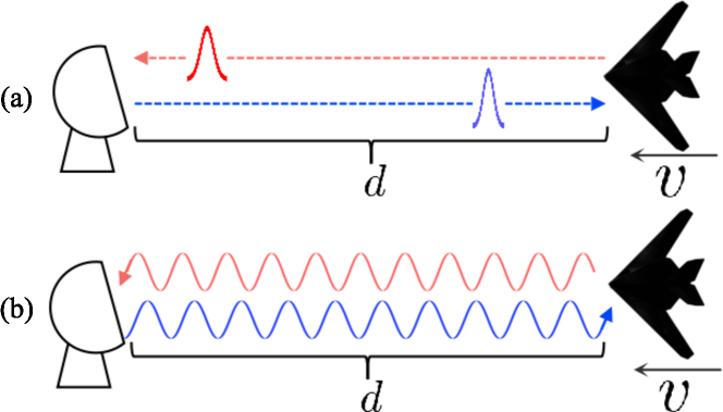
Figure 1: The sketches of (a) pulsed LiDAR and (b) FMCW LiDAR.

In addition to pulsed LiDAR, frequency modulated continuous wave (FMCW) technology can also be used to perform LiDAR operations, as Fig. 1 (b) shown. In contrast to pulsed LiDAR, FMCW LiDAR may receive signals constantly, eliminating the delay between pulses and eliminating the need for a minimum detection distance [19]. By coherently combining echo and reference light to create a beat signal, FMCW LiDAR can estimate range and velocity at the same time [20, 21, 22]. Moreover, FMCW LiDAR is more resistant to background noise [23, 24] and better suited for on-chip integration [25, 26, 27].

We study a quantum LiDAR with FMCW in this letter, which has three main contributions. We first present a scheme for the quantum-enhanced FMCW LiDAR, which is fundamentally different from the quantum pulsed LiDAR. This scheme involves a quantum FMCW light field of $n$-entangled photons with frequency modulation in a Mach-Zehnder (MZ) interferometer. By utilizing the entanglement among both the time and path, it improves the precision limit by $\sqrt{n}$ and the resolution by $n$ over the classical counterpart for the measurement of range and velocity. Second, using triangle frequency modulation, the quantum FMCW LiDAR enables the decoupling of range and velocity measurements. This makes it possible to estimate the target’s position and speed at the same time without using a quantum pulsed compression system like a quantum pulsed LiDAR. Finally, the quantum FMCW LiDAR system is better suited for practical implementation. In addition to the ability of the quantum FMCW LiDAR’s beat signal to down-convert the optical frequency enabling a more precise and compact electronic measurement of Doppler shift, the only inefficient nonlinear optical process that the system uses are the creation of the entangled photons. As a result, the system is easily applicable to integrated photonic platforms, such as thin film lithium niobite [28, 29, 30], which can effectively generate, manipulate, and detect quantum signals.

We first present the basic working principle of the FMCW LiDAR, then extend it to the quantum FMCW LiDAR.

The FMCW LiDAR measures the range and velocity of the object by sending frequency modulated continuous wave and detecting the echo light that bounces back from the object [20]. The echo light has a time delay, denoted as $\tau$, which is related to the target’s distance ($d$), and a Doppler shift ($\omega_{d}$), which is related to the object’s relative radial velocity ($v$). The velocity and range can then be determined by contrasting the reference light with the echo light. A widely used frequency modulation is the triangle frequency modulation, where the frequency of the continuous wave first increases, then decreases linearly, as shown in Fig.2. In this case the time of flight and the Doppler shift can be obtained as

$$\tau =\frac{2d}{c}=\frac{T_{m}}{2\Delta\omega}\frac{\omega_{b_{1}}+|\omega_{b_{2}}|}{2},$$ (1)

$$\omega_{d} =\omega_{c}\frac{2v}{c}=\frac{\omega_{b_{1}}-|\omega_{b_{2}}|}{2},$$

here $T_{m}$ is the period of modulation, $c>>v$ is the speed of light, and $\omega_{c}$ is the center frequency of the FMCW light field, $\omega_{b_{1}}$ and $\omega_{b_{2}}$ are the frequency differences between the reference light and the echo light at the rising and falling edges respectively, as shown in Fig. 2. $\omega_{b_{1}}$ and $\omega_{b_{2}}$, which are the frequencies of the beat signal produced by mixing the reference light and the echo light, can then be used to determine the range and velocity.

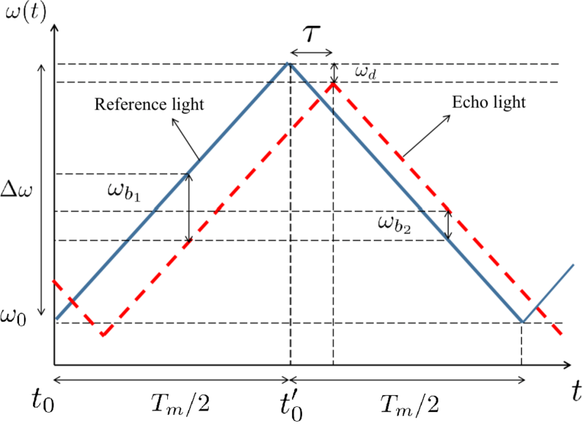
Figure 2: The variation of angular frequency $\omega(t)$ of the reference light and the echo light under the triangle frequency modulation with an initial modulation time $t_{0}=t^{\prime}_{0}-T_{m}/2$. For the reference light, $\omega(t)=\frac{\Delta\omega}{T_{m}/2}\left(t-t^{\prime}_{0}\right)+(\omega_{0}+\Delta\omega)$ in rising edge with a initial angular frequency $\omega_{0}$ and $\omega(t)=-\frac{\Delta\omega}{T_{m}/2}\left(t-t^{\prime}_{0}\right)+(\omega_{0}+\Delta\omega)$ in falling edge with a initial angular frequency $\omega_{0}+\Delta\omega$. $T_{m}$ and $\Delta\omega$ are modulation period and bandwidth respectively

The phase of the beat signal also depends on the relative distance as $\theta\propto\omega_{c}\tau=2\pi d/\lambda_{c}$ (see Sec. IB of the supplemental material), where $\lambda_{c}$ is the center wavelength of the FMCW light field. We include the phase of the beat signal, $\theta_{0(1)}$ in the rising (falling) edge, in the parameters to be estimated in addition to the beat frequencies to account for the effects on the precision for the estimation of frequencies in the presence of the unknown phases. It’s important to keep in mind that $\theta_{0(1)}$ depends on the initial time selections made for the rising and falling edges. The phase changes by $2\pi$ when the echo light travels a distance of one wavelength, making it highly sensitive to the relative distance. This property can be used to make detailed contours of the target’s surface by measuring a set of $\theta$ from different points on the surface, similar to interferometric imaging with monochromatic light [31, 32].

In classical optics, an optical FMCW beam can be described as an oscillating electromagnetic field $E_{\omega_{c}}(r,t)$ as

$$E_{\omega_{c}}(r,t)\propto E_{\omega_{c}}(t)=\alpha e^{i\int_{t_{0}}^{t}\omega(t)dt},$$ (2)

where $\alpha$, $\omega(t)$ and $\omega_{c}$ are the amplitude, modulating frequency and the center frequency respectively. Here for simplicity we consider a single spatial and polarization mode. When the field is modulated periodically, it can be decomposed into discrete frequencies with a spectrum $s_{\omega_{c}}(\omega_{j})=\frac{1}{T_{m}}\int_{t_{0}}^{t_{0}+T_{m}}dtE_{\omega_{c}}(t)e^{-i\omega_{j}t}$, $\omega_{j}=2\pi j/T_{m}$ with $j\in\{0,1,2,\ldots,\infty\}$.

In quantum optics, the classical light can be described by a coherent light $|\alpha(\omega)\rangle$. The frequency modulation transforms the coherent state to a FMCW coherent state $\mathop{\otimes}_{j}\left|\alpha s_{\omega_{c}}^{*}\left(\omega_{j}\right)\right\rangle$ with

$$\hat{a}^{+}(\omega)\rightarrow\sum^{\infty}_{j=0}s_{\omega_{c}}^{*}\left(\omega_{j}\right)\hat{a}^{+}\left(\omega_{j}\right),$$ (3)

here $s(\omega_{j})$ is a normalized complex spectrum with $\sum_{j}|s_{\omega_{c}}^{*}\left(\omega_{j}\right)|^{2}=1$ [33, 34]. Under the slowly-varying envelope approximation ($\omega_{c}>>\Delta\omega$) [35], the classical FMCW light field $E_{\omega_{c}}(t)$ can be described by a multi-mode coherent state $\mathop{\otimes}_{j}\left|\alpha s_{\omega_{c}}^{*}\left(\omega_{j}\right)\right\rangle$ with

$$\hat{E}^{(+)}(t)\propto\sum^{\infty}_{j=0}\hat{a}(\omega_{j})e^{-i\omega_{j}t},$$ (4)

where $\hat{a}(\omega_{j})$ and $\hat{a}^{+}(\omega_{j})$ are annihilation and creation operator.

We use finite bandwidth and discrete time approximations to model the quantum FMCW field in the time domain. In these approximations, a period of modulation, $T_{m}$, is divided into $j_{B}$ intervals with $j_{B}+1$ discrete time points. The annihilation operator at time $t_{p}$, the $p$-th discrete time point, is given by

$$\hat{a}(t_{p})\equiv\frac{1}{\sqrt{j_{B}+1}}\sum_{j=j_{c}-\frac{j_{B}}{2}}^{j_{c}+\frac{j_{B}}{2}}\hat{a}\left(\omega_{j}\right)e^{-i\omega_{j}t_{p}},$$ (5)

where $\omega_{j_{B}}=2\pi j_{B}/T_{m}$ is the finite bandwidth with $\omega_{j_{B}}\gg\Delta\omega$, $\omega_{j_{c}}$ represents a frequency closest to the central frequency of the FMCW light fields and $t_{p}=pT_{m}/j_{B}$ where $p\in\{p_{0},p_{0}+1,p_{0}+2,\dots,p_{0}+j_{B}\}$ with the initial time point $p_{0}\in\mathbb{Z}$. Due to periodicity, we have $\hat{a}(t_{p}+T_{m})=\hat{a}(t_{p})$. A Fock state in the time domain can then be written as

$$\left|n_{t_{p}}\right\rangle=\frac{1}{\sqrt{n_{t_{p}}!}}\left[\hat{a}^{+}(t_{p})\right]^{n_{t_{p}}}|0\rangle,$$ (6)

where $n_{t_{p}}$ is the photon number at $t_{p}$. As $[\hat{a}(t_{p}),\hat{a}^{\dagger}(t_{p^{\prime}})]=\delta_{p,p^{\prime}}$, the band-limited Hilbert space can be spanned by the discrete time mode $I=\otimes_{t_{p}}\sum_{n_{t_{p}}}\left|n_{t_{p}}\right\rangle\left\langle n_{t_{p}}\right|=\sum_{\mathbf{n}}\left|\mathbf{n}\right\rangle\left\langle\mathbf{n}\right|$, where $|\mathbf{n}\rangle=|n_{t_{p_{0}}},\ldots,n_{t_{{p_{0}+j_{B}}}}\rangle$ is a photon number state within a period.

Under the finite bandwidth and discrete time approximation, the single photon state of FMCW in the frequency domain, $\sum_{j=0}^{\infty}s_{\omega_{c}}^{*}\left(\omega_{j}\right)\hat{a}^{+}\left(\omega_{j}\right)|0\rangle$, can be transformed to the time domain as

$$|\psi_{1}\rangle\approx\frac{1}{\sqrt{j_{B}+1}}\sum_{p=p_{0}}^{p_{0}+j_{B}}E_{\omega_{c}}^{*}\left(t_{p}\right)\hat{a}^{+}\left(t_{p}\right)|0\rangle,$$ (7)

where $E_{\omega_{c}}\left(t_{p}\right)$ is the FMCW field given in Eq. (4) represented in the discrete time domain, $\omega_{c}$ is the center angular frequency, and $j_{B}$ is taken sufficiently large to include most frequency bands of the FMCW field. It can be seen that the single FMCW photon state in the time domain is typically a superposition of states at different times. For a two-photon anti-frequency-correlation entangled state [29, 30, 36] with a Gaussian correlation spectrum $G(\omega)$ with standard deviation $\sigma$, given by $\int d\omega G(\omega)\hat{a}_{1}^{+}\left(\omega_{c}+\omega\right)\hat{a}_{2}^{+}\left(\omega_{c}-\omega\right)|0\rangle$, the state of FMCW in the time domain is

$$|\psi_{2}\rangle\approx\frac{1}{j_{B}+1}\sum^{p_{0}+j_{B}}_{p,q=p_{0}}\tilde{G}\left(t_{p}-t_{q}\right)E_{\omega_{c}}\left(t_{p}\right)E_{\omega_{c}}\left(t_{q}\right)\times$$ (8)

$$\hskip 142.26378pt\hat{a}_{1}^{+}\left(t_{p}\right)\hat{a}_{2}^{+}\left(t_{q}\right)|0\rangle,$$

where $\tilde{G}\left(t\right)$ is the Fourier transformation of $G(\omega)$. We note that the phases of the frequency-modulated biphoton are correlated at different time points, known as chirp entanglement. The preparation of $|\psi_{2}\rangle$ is discussed in Sec. V of the supplemental material.

The quantum FMCW LiDAR is achieved by using part of the entangled state as the signal light and the other part as the reference light. A beating signal is then obtained from the interference between the echo light, that is reflected back from the target, and the reference light.

In general the $n$-photon FMCW NOON state can be used, where the signal can be represented as

$$\left|\psi_{n}(\vec{x})\right\rangle=\frac{1}{\sqrt{2T_{m}}}\int^{t_{0}+T_{m}}_{t_{0}}dt \left\{E_{\omega_{c}}^{*n}(t)\left|n_{t},0\right\rangle-\right.$$ (9)

$$\left.E_{\omega_{c}-\omega_{d}}^{*n}(t-\tau)\left|0,n_{t}\right\rangle\right\},$$

where the time delay $\tau$ and the Doppler shift $\omega_{d}$ are encoded in the echo light, $\vec{x}$ denotes the collections of the parameters to be estimated. To extract the information from $\left|\psi_{n}(\bm{O})\right\rangle$, an interferometric detection strategy

$$\hat{A}_{D}(t)=-(|n_{t},0\rangle\langle 0,n_{t}|+|0,n_{t}\rangle\langle n_{t},0|),$$ (10)

can be applied at each time when photons are detected. This detection strategy keeps track of the probability of projecting on the two eigenstates of $\hat{A}_{D}(t)$, which forms the quantum beating signal.

The schematic physical implementation of quantum FMCW LiDAR scheme, for $n=1$ (for comparison) and $n=2$, is shown in Fig. 3. It is similar to the MZ interferometer but with two differences. First, the target is always been placed in the middle of one arm to create specular-like reflection that simulates the round-trip propagation of the echo light. Second, the evolution of the light field is described with the frequency-independent time of light ($\tau(t)\approx\tau+(\omega_{d}/\omega_{c})t=2(d+vt)/c$ (if $|v|<<c$)) [37] instead of the frequency-dependent phase differences that is typically used in the MZ interferometer. The details of the derivation of the evolution and detection can be found in Sec. IIC and Sec. IID of the supplemental material.

A scheme of using bi-photon NOON state, $|\psi_{2}\rangle$, is sketched in Fig. 3. After the BS1 and the free evolution, the state $|\psi_{2}\rangle$ becomes

$$|\psi_{2}(\vec{x})\rangle=\frac{1}{2\left(n_{B}+1\right)}\sum^{p_{0}+j_{B}}_{p,q=p_{0}}\tilde{G}\left(t_{p}-t_{q}\right)\times$$ (11)

$$\left\{E_{\omega_{c}}^{*}\left(t_{p}\right)E_{\omega_{c}}^{*}\left(t_{q}\right)\hat{a}_{R}^{+}\left(t_{p}\right)\hat{a}_{R}^{+}\left(t_{q}\right)-\right.$$

$$\enspace\left.E_{\omega_{c}-\omega_{d}}^{*}\left(t_{p}-\tau\right)E_{\omega_{c}-\omega_{d}}^{*}\left(t_{q}-\tau\right)\hat{a}_{T}^{+}\left(t_{p}\right)\hat{a}_{T}^{+}\left(t_{q}\right)\right\}|0\rangle$$

showing both path and chirp entanglements.

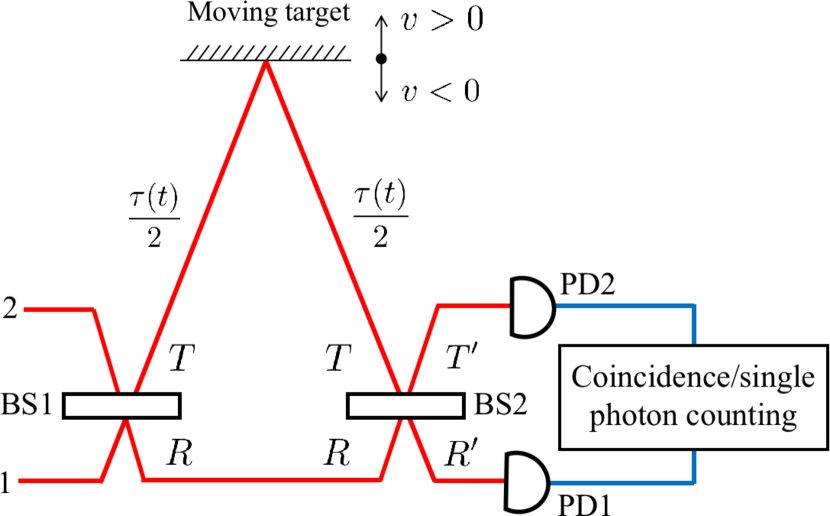
Figure 3: The sketches of target ranging and velocity measurement by using MZ interferometer. The BS1 (BS2) and the PD1 (PD2) are the 50:50 beam splitter and the photon detector respectively. If the FMCW single photon state $|\psi_{1}\rangle$ input from port 1, the single photon counting is applied. If the FMCW biphoton entangled state $|\psi_{2}\rangle$ are input from port 1 and port 2 simultaneously, the coincidence photon counting is applied. The target velocity $v>0$ ($v<0$) when the target is moving away (toward) from the photon detectors which creates a red (blue) shift.

At the detection side, two photon counters are used to keep track of the variation of joint detection probability with time. This is the second order quantum correlation function

$$\langle\psi_{2}(\vec{x})|\hat{E}_{R^{\prime}}^{(-)}\left(t_{1}\right)\hat{E}_{T^{\prime}}^{(-)}\left(t_{2}\right)\hat{E}_{T^{\prime}}^{(+)}\left(t_{2}\right)\hat{E}_{R^{\prime}}^{(+)}\left(t_{1}\right)|\psi_{2}(\vec{x})\rangle$$ (12)

with a time delay $\tau^{\prime}=t_{1}-t_{2}$. Given that the time delay is normally distributed as shown in Eq. (11), the probability of coincidence counting becomes

$$p_{2}\left(1\mid t,\vec{x}\right)=\int d\tau^{\prime} \langle\psi_{2}(\vec{x})|\hat{E}_{R^{\prime}}^{(-)}\left(t\right)\hat{E}_{T^{\prime}}^{(-)}\left(t-\tau^{\prime}\right)\times$$ (13)

$$\hat{E}_{T^{\prime}}^{(+)}\left(t-\tau^{\prime}\right)\hat{E}_{R^{\prime}}^{(+)}\left(t\right)|\psi_{2}(\vec{x})\rangle.$$

Here, one of the photon is detected by PD1 at time $t_{1}=t$ while the other photon is detected by PD2 with an arbitrary time delay. So the probability of both photons detected by the same detector (PD1 or PD2) is $p_{2}\left(0\mid t,\vec{x}\right)=1-p_{2}\left(1\mid t,\vec{x}\right)$.

For triangular modulation, the scheme yields a piece-wise detection probability distribution

$$\begin{aligned} &p_{n}\left(1\mid d,v,\theta_{l},t\right)\approx\\ &\quad\frac{1}{2}+\frac{1}{2}\cos\left\{n\left[(-1)^{l}\frac{\Delta\omega}{T_{m}/2}\frac{2d}{c}+\omega_{c}\frac{2v}{c}\right]t+n\theta_{l}\right\}\end{aligned},$$ (14)

where $l=0$ for $t\in[t_{d_{0}}-T_{m}/2,t_{d_{0}}]$, and $l=1$ for $t\in[t_{d_{1}},t_{d_{1}}+T_{m}/2]$. Here $n=1,2$ stand for the single photon and the two-photon entanglement states respectively. These detection probabilities oscillate with time, which form the quantum beat signals. The target distance $d$ and velocity $v$ can then be derived from the frequencies of the beat signal.

The precision limit for the estimation of $\vec{x}=\{d,v,\theta_{0},\theta_{1}\}$ can be quantified by the Cramer-Rao bound (CRB) with $Cov(\hat{x})\geq\frac{1}{\nu}F_{C}^{-1}[\vec{x}]$, where $Cov(\hat{x})$ is the covariance matrix for unbiased estimator, $\hat{x}$, and $F_{C}[\vec{x}]$ is the classical Fisher information (CFI) matrix, $\nu$ is the number of times the procedure is repeated. In a period of FMCW modulation, the instaneous $F_{C}[\vec{x},t]$ varies over time $t$. To get overall CFI, the contribution of CFI in the whole period should be considered, e.g., $F_{C}[\vec{x}]=\int^{t_{d_{0}}}_{t_{d_{0}}-T_{m}/2}dtF_{C}[\vec{x},t]+\int^{t_{d_{1}}+T_{m}/2}_{t_{d_{1}}}dtF_{C}[\vec{x},t]$. Further, in order to exclude the covariance between initial phase $\theta_{0,1}$ and the beat frequencies resulted from different $t_{d_{0}}$ and $t_{d_{1}}$ (see Sec. IIIB of the supplemental material) [38], it is set that $t_{d_{0}}=-t_{d_{1}}=T_{m}/4$.

We can explicitly calculate $F_{C}[\bm{O}]$ and obtain the CRB as

$$\operatorname{Cov}(\hat{x}) \geq\frac{1}{\nu}F^{-1}_{C}[\vec{x}]=$$ (15)

$$\frac{1}{\nu T_{m}} \begin{pmatrix}\frac{3}{n^{2}}\frac{c^{2}}{\Delta\omega^{2}}&0&0&0\\ \\ 0&\frac{12}{n^{2}}\frac{c^{2}}{\omega_{c}^{2}T_{m}^{2}}&0&0\\ \\ 0&0&\frac{2}{n^{2}}&0\\ \\ 0&0&0&\frac{2}{n^{2}}\end{pmatrix}.$$

With the same output power, the covariance matrix with entangled photon pairs ($n=2$) is half of the single photon case ($n=1$).

In the quantum FMCW LiDAR scheme, the resolution of $\{d,v\}$ is rooted in the discrete Fourier transform (DFT) of the measured quantum beating signal. The DFT corresponds to the maximum-likelihood (ML) estimators for $\vec{x}$ [38, 39]. The classical CRB can be achieved with this ML estimator [38]. Hence, the resolutions of $\{d,v\}$ is governed by the frequency resolution in the DFT. For the triangular modulation, if we perform the DFT independently on the beating signals, given in Eq. (14), at each half period, a frequency resolution of $\frac{2\pi}{T_{m}/2}$ can be achieved. This leads to the resolutions of $\{d,v\}$ as (see Sec.IIID of the supplemental material for detail):

$$\Delta d=\frac{2\pi}{n}\frac{c}{2\Delta\omega},\quad\Delta v=\frac{2\pi}{n}\frac{c}{\omega_{c}T_{m}}.$$ (16)

This shows an improvement on the resolution of $\{d,v\}$ by a factor of 2 when two-photon entangled states are used to replace the coherent states. In addition, the initial phase of the quantum beat signals are multiplied by two indicating that a phase resolution of $\{\theta_{0},\theta_{1}\}$ is improved by a factor of 2 [40]. Similar analysis can be extended to the scenario with $n$-photon entangled states with an improvement of a factor of $n$.

The quantum FMCW LiDAR that we studied in this letter is distinct from the conventional quantum pulsed LiDAR. A design of this scheme with entangled photon pairs ($n=2$) is illustrated with an MZ interferometer. The ability of the quantum FMCW LiDAR to detect range and velocity simultaneously with high precision is demonstrated. This is in contrast to the pulsed quantum LiDAR, which requires quantum pulsed compression.

Quantum FMCW LiDAR provides three main advantages over pulsed quantum LiDAR. First, unlike the quantum pulsed LiDAR, the quantum FMCW LiDAR does not require additional nonlinear optical processes to entangle or de-entangle photons in order to measure ranging and velocity simultaneously [14, 15]. Note that in order to produce the entangled state of light, both types of quantum LiDARs require nonlinear optical processes (such as spontaneous parametric down conversion). However, further nonlinear optical processes are needed for the quantum pulsed LiDAR to de-entangle the entangled pulsed light in order to measure the ToF and the Doppler shift separately. These nonlinear optical processes are also utilized to entangle various types of pulsed light in quantum pulsed LiDAR proposals [14], in order to produce entangled pulsed light with high time-bandwidth products. These nonlinear optical processes [41], however, are typically inefficient (see Sec. VI of the supplemental material). The quantum FMCW LiDAR is able to use quantum resources more efficiently, which is beneficial for key performance metrics, such as signal-to-noise ratio, measurement range, etc.

Second, the beat signals, which are normally in the microwave range and can be precisely measured by cutting-edge electronic circuitry, are used in the quantum FMCW LiDAR to extract the information. The operational frequency band is downconverted in this way, greatly increasing the scheme’s viability. Comparatively, the exact measurement of the time and the optical Doppler shift required by the quantum pulsed LiDAR can be challenging [17, 18].

Lastly, a significantly more compact architecture is made possible by the quantum FMCW LiDAR’s better suitability for on-chip integration. Since the quantum FMCW LiDAR’s peak power can be substantially lower than that of the pulsed LiDAR, it is more suited for integrated photonics. In fact, the beam splitter, modulation, and entangled light source of the on-chip quantum FMCW LiDAR have all been successfully demonstrated [29, 30] on the lithium niobite chip platform [28] with comparatively high efficiency.

The quantum FMCW LiDAR has a lot of benefits for practical implementations due to its energy efficiency, capability to analyze signals in the microwave spectrum, and appropriateness for on-chip integration. The approach can also be applied to other non-classical light fields [42, 43, 44, 45, 46, 47, 48, 49, 50, 51], such as the multimode squeezed-vacuum state [11], the photon-added coherent state [52, 53] and the optimal photon number state [54].

References

- Kim et al. [2021] I. Kim, R. J. Martins, J. Jang, T. Badloe, S. Khadir, H.-Y. Jung, H. Kim, J. Kim, P. Genevet, and J. Rho, Nanophotonics for light detection and ranging technology, Nature Nanotechnology 16, 508 (2021).
- Giovannetti et al. [2006] V. Giovannetti, S. Lloyd, and L. Maccone, Quantum Metrology, Physical Review Letters 96, 010401 (2006).
- Giovannetti et al. [2001] V. Giovannetti, S. Lloyd, and L. Maccone, Quantum-enhanced positioning and clock synchronization, Nature 412, 417 (2001).
- Giovannetti et al. [2002a] V. Giovannetti, S. Lloyd, and L. Maccone, Positioning and clock synchronization through entanglement, Physical Review A 65, 022309 (2002a).
- Maccone and Ren [2020] L. Maccone and C. Ren, Quantum Radar, Physical Review Letters 124, 200503 (2020).
- Lloyd [2008] S. Lloyd, Enhanced Sensitivity of Photodetection via Quantum Illumination, Science 321, 1463 (2008).
- Chang et al. [2019] C. W. S. Chang, A. M. Vadiraj, J. Bourassa, B. Balaji, and C. M. Wilson, Quantum-enhanced noise radar, Applied Physics Letters 114, 112601 (2019).
- Barzanjeh et al. [2015] S. Barzanjeh, S. Guha, C. Weedbrook, D. Vitali, J. H. Shapiro, and S. Pirandola, Microwave Quantum Illumination, Physical Review Letters 114, 080503 (2015).
- Zhuang [2021] Q. Zhuang, Quantum Ranging with Gaussian Entanglement, Physical Review Letters 126, 240501 (2021).
- Liu et al. [2019] H. Liu, D. Giovannini, H. He, D. England, B. J. Sussman, B. Balaji, and A. S. Helmy, Enhancing LIDAR performance metrics using continuous-wave photon-pair sources, Optica 6, 1349 (2019).
- Reichert et al. [2022] M. Reichert, R. Di Candia, M. Z. Win, and M. Sanz, Quantum-enhanced Doppler lidar, npj Quantum Information 8, 147 (2022).
- Shapiro [2007] J. H. Shapiro, Quantum pulse compression laser radar, in SPIE Fourth International Symposium on Fluctuations and Noise, edited by L. Cohen (Florence, Italy, 2007) p. 660306.
- Zhuang and Shapiro [2022] Q. Zhuang and J. H. Shapiro, Ultimate Accuracy Limit of Quantum Pulse-Compression Ranging, Physical Review Letters 128, 010501 (2022).
- Zhuang et al. [2017] Q. Zhuang, Z. Zhang, and J. H. Shapiro, Entanglement-enhanced lidars for simultaneous range and velocity measurements, Physical Review A 96, 040304 (2017).
- Huang et al. [2021] Z. Huang, C. Lupo, and P. Kok, Quantum-Limited Estimation of Range and Velocity, PRX Quantum 2, 030303 (2021).
- Blakey et al. [2022] P. S. Blakey, H. Liu, G. Papangelakis, Y. Zhang, Z. M. Léger, M. L. Iu, and A. S. Helmy, Quantum and non-local effects offer over 40 db noise resilience advantage towards quantum lidar, Nature Communications 13, 5633 (2022).
- Avenhaus et al. [2009] M. Avenhaus, A. Eckstein, P. J. Mosley, and C. Silberhorn, Fiber-assisted single-photon spectrograph, Optics Letters 34, 2873 (2009).
- Thekkadath et al. [2022] G. S. Thekkadath, B. A. Bell, R. B. Patel, M. S. Kim, and I. A. Walmsley, Measuring the joint spectral mode of photon pairs using intensity interferometry, Physical Review Letters 128, 023601 (2022), arxiv:2107.06244 [physics, physics:quant-ph] .
- Li and Shi [2022] Y. Li and H. Shi, Advanced Driver Assistance Systems and Autonomous Vehicles: From Fundamentals to Applications (Springer Nature, 2022).
- Zheng [2005] J. Zheng, Optical Frequency-Modulated Continuous-Wave (FMCW) Interferometry, Springer Series in Optical Sciences No. 107 (Springer, New York [Heidelberg], 2005).
- Riemensberger et al. [2020] J. Riemensberger, A. Lukashchuk, M. Karpov, W. Weng, E. Lucas, J. Liu, and T. J. Kippenberg, Massively parallel coherent laser ranging using a soliton microcomb, Nature 581, 164 (2020).
- Lukashchuk et al. [2022] A. Lukashchuk, J. Riemensberger, M. Karpov, J. Liu, and T. J. Kippenberg, Dual chirped microcomb based parallel ranging at megapixel-line rates, Nature Communications 13, 3280 (2022).
- Qian et al. [2022] R. Qian, K. C. Zhou, J. Zhang, C. Viehland, A.-H. Dhalla, and J. A. Izatt, Video-rate high-precision time-frequency multiplexed 3D coherent ranging, Nature Communications 13, 1476 (2022).
- Hsu et al. [2022] C.-Y. Hsu, G.-Z. Yiu, and Y.-C. Chang, Free-Space Applications of Silicon Photonics: A Review, Micromachines 13, 990 (2022).
- Behroozpour et al. [2017] B. Behroozpour, P. A. M. Sandborn, M. C. Wu, and B. E. Boser, Lidar System Architectures and Circuits, IEEE Communications Magazine 55, 135 (2017).
- Zhang et al. [2022] X. Zhang, K. Kwon, J. Henriksson, J. Luo, and M. C. Wu, A large-scale microelectromechanical-systems-based silicon photonics LiDAR, Nature 603, 253 (2022).
- Lihachev et al. [2022] G. Lihachev, J. Riemensberger, W. Weng, J. Liu, H. Tian, A. Siddharth, V. Snigirev, V. Shadymov, A. Voloshin, R. N. Wang, J. He, S. A. Bhave, and T. J. Kippenberg, Low-noise frequency-agile photonic integrated lasers for coherent ranging, Nature Communications 13, 3522 (2022).
- Zhu et al. [2021] D. Zhu, L. Shao, M. Yu, R. Cheng, B. Desiatov, C. J. Xin, Y. Hu, J. Holzgrafe, S. Ghosh, A. Shams-Ansari, E. Puma, N. Sinclair, C. Reimer, M. Zhang, and M. Lončar, Integrated photonics on thin-film lithium niobate, Advances in Optics and Photonics 13, 242 (2021).
- Jin et al. [2014] H. Jin, F. M. Liu, P. Xu, J. L. Xia, M. L. Zhong, Y. Yuan, J. W. Zhou, Y. X. Gong, W. Wang, and S. N. Zhu, On-Chip Generation and Manipulation of Entangled Photons Based on Reconfigurable Lithium-Niobate Waveguide Circuits, Physical Review Letters 113, 103601 (2014).
- Xue et al. [2021] G.-T. Xue, Y.-F. Niu, X. Liu, J.-C. Duan, W. Chen, Y. Pan, K. Jia, X. Wang, H.-Y. Liu, Y. Zhang, P. Xu, G. Zhao, X. Cai, Y.-X. Gong, X. Hu, Z. Xie, and S. Zhu, Ultrabright Multiplexed Energy-Time-Entangled Photon Generation from Lithium Niobate on Insulator Chip, Physical Review Applied 15, 064059 (2021).
- Turbide et al. [2012] S. Turbide, L. Marchese, M. Terroux, F. Babin, and A. Bergeron, An all-optronic synthetic aperture lidar, in SPIE Security + Defence, edited by G. W. Kamerman, O. Steinvall, G. J. Bishop, J. Gonglewski, K. L. Lewis, R. C. Hollins, T. J. Merlet, M. T. Gruneisen, M. Dusek, and J. G. Rarity (Edinburgh, United Kingdom, 2012) p. 854213.
- Terroux et al. [2017] M. Terroux, A. Bergeron, S. Turbide, and L. Marchese, Synthetic aperture lidar as a future tool for earth observation, in International Conference on Space Optics — ICSO 2014, edited by B. Cugny, Z. Sodnik, and N. Karafolas (SPIE, Tenerife, Canary Islands, Spain, 2017) p. 196.
- Capmany and Fernández-Pousa [2010] J. Capmany and C. R. Fernández-Pousa, Quantum model for electro-optical phase modulation, Journal of the Optical Society of America B 27, A119 (2010).
- Capmany and Fernández-Pousa [2011] J. Capmany and C. Fernández-Pousa, Quantum modelling of electro-optic modulators, Laser & Photonics Reviews 5, 750 (2011).
- Tsang et al. [2008] M. Tsang, J. H. Shapiro, and S. Lloyd, Quantum theory of optical temporal phase and instantaneous frequency, Physical Review A 78, 053820 (2008).
- Giovannetti et al. [2002b] V. Giovannetti, L. Maccone, J. H. Shapiro, and F. N. C. Wong, Extended phase-matching conditions for improved entanglement generation, Physical Review A 66, 043813 (2002b).
- Ivanov et al. [2020] S. Ivanov, V. Kuptsov, V. Badenko, and A. Fedotov, An Elaborated Signal Model for Simultaneous Range and Vector Velocity Estimation in FMCW Radar, Sensors 20, 5860 (2020).
- Rife and Boorstyn [1974] D. Rife and R. Boorstyn, Single tone parameter estimation from discrete-time observations, IEEE Transactions on Information Theory 20, 591 (1974).
- Erkmen et al. [2013] B. I. Erkmen, Z. W. Barber, and J. Dahl, Maximum-likelihood estimation for frequency-modulated continuous-wave laser ranging using photon-counting detectors, Applied Optics 52, 2008 (2013).
- Boto et al. [2000] A. N. Boto, P. Kok, D. S. Abrams, S. L. Braunstein, C. P. Williams, and J. P. Dowling, Quantum Interferometric Optical Lithography: Exploiting Entanglement to Beat the Diffraction Limit, Physical Review Letters 85, 2733 (2000).
- Couteau [2018] C. Couteau, Spontaneous parametric down-conversion, Contemporary Physics 59, 291 (2018).
- Plick et al. [2010] W. N. Plick, P. M. Anisimov, J. P. Dowling, H. Lee, and G. S. Agarwal, Parity detection in quantum optical metrology without number-resolving detectors, New Journal of Physics 12, 113025 (2010).
- Kacprowicz et al. [2010] M. Kacprowicz, R. Demkowicz-Dobrzański, W. Wasilewski, K. Banaszek, and I. A. Walmsley, Experimental quantum-enhanced estimation of a lossy phase shift, Nature Photonics 4, 357 (2010).
- Sahota and James [2013] J. Sahota and D. F. V. James, Quantum-enhanced phase estimation with an amplified Bell state, Physical Review A 88, 063820 (2013).
- Sahota and Quesada [2015] J. Sahota and N. Quesada, Quantum correlations in optical metrology: Heisenberg-limited phase estimation without mode entanglement, Physical Review A 91, 013808 (2015).
- Larson and Saleh [2017] W. Larson and B. E. A. Saleh, Supersensitive ancilla-based adaptive quantum phase estimation, Physical Review A 96, 042110 (2017).
- Zhang et al. [2019] J.-D. Zhang, Z.-J. Zhang, L.-Z. Cen, J.-Y. Hu, and Y. Zhao, Nonlinear phase estimation: Parity measurement approaches the quantum Cramér-Rao bound for coherent states, Physical Review A 99, 022106 (2019).
- Alodjants et al. [2022] A. Alodjants, D. Tsarev, T. V. Ngo, and R.-K. Lee, Enhanced nonlinear quantum metrology with weakly coupled solitons in the presence of particle losses, Physical Review A 105, 012606 (2022).
- Yu et al. [2020] J. Yu, Y. Qin, J. Qin, H. Wang, Z. Yan, X. Jia, and K. Peng, Quantum Enhanced Optical Phase Estimation With a Squeezed Thermal State, Physical Review Applied 13, 024037 (2020).
- Zhang et al. [2021] H. Zhang, W. Ye, C. Wei, C. Liu, Z. Liao, and L. Hu, Improving phase estimation using number-conserving operations, Physical Review A 103, 052602 (2021).
- Gatto et al. [2022] D. Gatto, P. Facchi, and V. Tamma, Heisenberg-limited estimation robust to photon losses in a Mach-Zehnder network with squeezed light, Physical Review A 105, 012607 (2022).
- Agarwal and Tara [1991] G. S. Agarwal and K. Tara, Nonclassical properties of states generated by the excitations on a coherent state, Physical Review A 43, 492 (1991).
- Francis and Tame [2020] J. T. Francis and M. S. Tame, Photon-added coherent states using the continuous-mode formalism, Physical Review A 102, 043709 (2020).
- Dorner et al. [2009] U. Dorner, R. Demkowicz-Dobrzanski, B. J. Smith, J. S. Lundeen, W. Wasilewski, K. Banaszek, and I. A. Walmsley, Optimal Quantum Phase Estimation, Physical Review Letters 102, 040403 (2009).