Data-based system representations from irregularly measured data

Abstract

Non-parametric representations of dynamical systems based on the image of a Hankel matrix of data are extensively used for data-driven control. However, if samples of data are missing, obtaining such representations becomes a difficult task. By exploiting the kernel structure of Hankel matrices of irregularly measured data generated by a linear time-invariant system, we provide computational methods for which any complete finite-length behavior of the system can be obtained. For the special case of periodically missing outputs, we provide conditions on the input such that the former result is guaranteed. We illustrate with an example how the resulting representation provides a more computationally efficient method for low-rank matrix completion when compared to an alternative method.

I Introduction

Many systems of interest are too complicated to model using first principles. However, abundance of data generated from such systems and recent advances in machine learning are opening new research possibilities for modeling and control design. Data- and learning-based models of dynamical systems can be obtained using, e.g., Neural networks [1], Gaussian processes [2], or other machine learning techniques. Alternatively, the behavioral approach to dynamical systems theory [3] exploits system properties to arrive at non-parametric models of dynamical systems.

A recently revived and celebrated result from the behavioral framework is the so-called fundamental lemma [4]. This lemma provides a non-parametric representation of the finite-length behavior of a discrete-time LTI system as the image of a Hankel matrix of a single persistently exciting (PE) trajectory. In particular, it asserts that any trajectory of an LTI system is given by a linear combination of time-shifts of a single measured trajectory. This result is central to several works on direct data-based control for linear [5, 6, 7, 8] and nonlinear systems [9, 10, 11]. The reader is referred to [12] for a comprehensive review.

Essential to [4] and all subsequent results that build on it is that the collected data is consecutive or made up of multiple sufficiently long trajectories of the system (see [6]). However, in practice data can be missing due to several reasons, e.g., sensor failure and/or (irregular) packet losses in networked control systems [13]. It also might not be possible to measure some states regularly, e.g., in biomedical applications [14]. This motivates the development of non-parametric representations of dynamical systems from irregularly measured data, which can then be used for system analysis and control design.

In [15], the authors use consecutive offline input/state data of discrete-time LTI systems to design stabilizing controllers for closed-loop aperiodically sampled systems. In [16], methods to complete data sequences with missing samples are proposed by formulating data-driven approximation and interpolation problems. Both of these works still assume the availability of complete data sequences collected offline and, hence, a non-parametric model of the system is assumed to be available (cf. [4]). The case where data is (regularly or irregularly) missing in the offline phase is not discussed. The goal of this paper is to exploit the kernel structure of Hankel matrices [17, 18] in order to retrieve a non-parametric representation of the finite-length behavior of an LTI system using the available (irregularly measured) data.

In the system identification literature, missing data has been addressed in several works. The methods used include frequency domain tools [19], local optimization methods [20] and convex relaxations based on nuclear norm minimization [21]. In this work, we address the problem using the language of the behavioral framework [3], as was done in [22, 23]. There, a dynamical system is viewed as a set of trajectories, allowing us to define the system properties in terms of its behavior. A representation of the system, however, is defined independently from its behavior and one of several representations of a dynamical system is the kernel representation. Identifying the minimal kernel representation of scalar systems despite missing data was addressed in [22, 23]. There, a search algorithm was proposed to select submatrices of the Hankel matrix of data and use them to reconstruct the minimal kernel representation of the system. However, no conditions were given to guarantee that this algorithm succeeds for any pattern of missing data.

The contributions of this paper are as follows:

• We first modify the algorithm in [22, 23] and use it to obtain a kernel representation of multivariable systems using irregularly measured data.

• We then exploit the kernel structure of Hankel matrices to recover any complete finite-length behavior of the system, i.e., we recover a non-parametric model of the system similar to the one given by the fundamental lemma [4]

• We consider the special case of periodically missing outputs and provide sufficient conditions on the input such that a kernel representation is guaranteed to be retrieved from the available data. This allows us to propose a fundamental-lemma-like result using data with periodically missing outputs.

The remainder of the paper is organized as follows: Section II introduces the notation and reviews preliminary results. Section III formulates the problem of finding kernel representations from missing data, and includes the corresponding algorithm required to compute them. Section IV shows how to use these representations in order to obtain a non-parametric representation of any complete finite-length behavior of the system, by exploiting the kernel structure of Hankel matrices. Section V focuses on the special case of periodically missing outputs and provides conditions on the input such that a fundamental-lemma-like result is obtained. Section VI verifies the results using numerical examples and illustrates how the resulting representation provides a computationally more efficient method for low-rank matrix completion when compared to convex relaxations of this problem based on the nuclear norm minimization (see [21]). Finally, Section VII discusses the results and concludes the paper.

II Preliminaries

The sets of integers, natural and real numbers are denoted by $\mathbb{Z},\mathbb{N},\mathbb{R}$, respectively. The restriction of integers to an interval is denoted by $\mathbb{Z}_{[a,b]}$ for $b>a\in\mathbb{Z}$. We use $I_{m}$ to denote an $m\times m$ identity matrix and $0_{n\times m}$ to denote an $n\times m$ matrix of zeros; when the dimensions are clear from the context, we omit the subscript for simplicity. We use $\lfloor z\rfloor$ to denote the floor operator which acts on $z\in\mathbb{R}$ and returns the greatest integer less than or equal to $z$. For a matrix $M\in\mathbb{R}^{m\times n}$, we denote its image by im$(M)$ and its kernel by ker$(M)$. When a basis of ker$(M)$ is to be computed, we write $N=~{}\textup{null}(M)$ which returns a matrix $N$ of appropriate dimensions such that $MN=~{}0$. The set of polynomial matrices (in $z$) with coefficients in $\mathbb{R}^{m\times n}$ is denoted by $\mathbb{R}^{m\times n}[z]$. For a subspace $\mathcal{A}$ of $\mathbb{R}^{n}$, we denote its orthogonal complement by $\mathcal{A}^{\perp}$. Further, for another subspace $\mathcal{B}$ of $\mathbb{R}^{n}$ such that $\mathcal{A}\cap\mathcal{B}=\{0\}$, the direct sum of the two subspaces is denoted by $\mathcal{A}\oplus\mathcal{B}$.

The set of infinite length $q-$variate, real-valued time series $w=(w(0),w(1),\ldots)$ is denoted by $\left(\mathbb{R}^{q}\right)^{\mathbb{N}}$. For $T\in\mathbb{N}$, the set of finite-length $q-$variate, real-valued time series $w=(w(0),w(1),\ldots,w(T-1))$ is denoted by $\left(\mathbb{R}^{q}\right)^{T}$. With slight abuse of notation, we also use $w$ to denote the stacked vector of the time series as

$$w=\begin{bmatrix}(w(0))^{\top}&(w(1))^{\top}&\cdots&(w(T-1))^{\top}\end{bmatrix}^{\top}\in~{}\mathbb{R}^{qT},$$

and its restriction to $L$ as

$$w_{[0,L-1]}=\begin{bmatrix}(w(0))^{\top}&(w(1))^{\top}&\cdots&(w(L-1))^{\top}\end{bmatrix}^{\top}\in\mathbb{R}^{qL}.$$

The Hankel matrix of depth $L$ of $w$ is defined as

$$\mathscr{H}_{L}(w)=\begin{bmatrix}w(0)&w(1)&\cdots&w(T-L)\\ w(1)&w(2)&\cdots&w(T-L+1)\\ \vdots&\vdots&\ddots&\vdots\\ w(L-1)&w(L)&\cdots&w(T-1)\end{bmatrix}.$$

The behavior $\mathscr{B}$ of a dynamical system is defined as a set of infinite-length trajectories (cf. [3]). The finite-length behavior of a system is a set of finite-length trajectories. For $T\in\mathbb{N}$, this is denoted by $\left.\mathscr{B}\right|_{T}$ and, hence, a trajectory of length $T$ of the system is denoted by $w\in\left.\mathscr{B}\right|_{T}\subset\left(\mathbb{R}^{q}\right)^{T}$. The system is linear if $\mathscr{B}$ is a subspace (of $\left(\mathbb{R}^{q}\right)^{\mathbb{N}}$) and it is time-invariant if it is invariant to the action of the shift operator, which is defined as $\sigma:\left(\mathbb{R}^{q}\right)^{\mathbb{N}}\to\left(\mathbb{R}^{q}\right)^{\mathbb{N}}$ such that $\sigma^{j}w(k)\coloneqq w(k+j)$ for $j\in\mathbb{N}$.

Let $u(t)\in\mathbb{R}^{m}$ and $y(t)\in\mathbb{R}^{p}$ denote the inputs and outputs of system $\mathscr{B}$ at time $t$. For a permutation matrix $\Pi\in\mathbb{R}^{q\times q}$, we define a partitioning of the variable $w(t)\in\mathbb{R}^{q}$ such that $w(t)=\Pi\begin{bmatrix}u(t)\\ y(t)\end{bmatrix}$. The set of discrete-time LTI systems with $q-$variables and fixed complexity $(m,n,\ell)$ is denoted by $\partial\mathscr{L}_{m,n,\ell}^{q}$, where $q=m+p$ and $(m,n,\ell)$ denote (i) the number of inputs $\textbf{m}(\mathscr{B})=m$, (ii) the order of the system $\textbf{n}(\mathscr{B})=n$, and (iii) the lag of the system $\boldsymbol{\ell}(\mathscr{B})=\ell$, which is the observability index in the state-space framework. These integers satisfy the following relation $\ell\leq n\leq p\ell$ [24].

A finite-dimensional LTI system $\mathscr{B}\in\partial\mathscr{L}_{m,n,\ell}^{q}$ admits a kernel representation [3, Part I]

$$\mathscr{B}=\textup{ ker }R(\sigma)\coloneqq\{w:\mathbb{N}\to\mathbb{R}^{q}~{}|~{}R(\sigma)w=0\},$$ (1)

where the operator $R(\sigma)$ is defined by the polynomial matrix

$$R(z) =R_{0}+R_{1}z+\ldots+R_{\ell}z^{\ell}$$ (2)

$$=\begin{bmatrix}r_{1}(z)\\ \vdots\\ r_{g}(z)\end{bmatrix}=\begin{bmatrix}r_{1,0}+r_{1,1}z+\ldots+r_{1,\ell_{1}}z^{\ell_{1}}\\ \vdots\\ r_{g,0}+r_{g,1}z+\ldots+r_{g,\ell_{g}}z^{\ell_{g}}\end{bmatrix}\in\mathbb{R}^{g\times q}[z],$$

with $r_{i,j}\in\mathbb{R}^{1\times q}$. A minimal kernel representation is one where the degree of the polynomial matrix $R$ is minimal. Each row $r_{i}(z)$ of $R(z)$ defines an annihilator $r(\sigma)$ of the system and is formally defined as follows.

Definition 1.

[24, Def. 2] An annihilator of $\mathscr{B}\in\partial\mathscr{L}_{m,n,\ell}^{q}$ is an operator $r(\sigma)$, $r(z)\in\mathbb{R}^{1\times q}[z]$, such that $r(\sigma)\mathscr{B}=0$.

A finite dimensional LTI system $\mathscr{B}\in\partial\mathscr{L}_{m,n,\ell}^{q}$ also admits an input/state/output representation of the form

$$\mathscr{B} =\mathscr{B}_{ss}(A,B,C,D,\Pi)\coloneqq\left\{\Pi\begin{bmatrix}u\\ y\end{bmatrix}~{}|~{}\exists x\in(\mathbb{R}^{n})^{\mathbb{N}},\right.$$ (3)

$$\quad\left.\textup{s.t.}\quad\sigma x=Ax+Bu,\,y=Cx+Du\right\}.$$

One of the key ideas in the behavioral framework is the notion of the most powerful unfalsified model (MPUM) of the data [3, Part II], denoted $\mathscr{B}_{\textup{MPUM}}$. The MPUM always exists and is unique. Its restricted behavior, i.e., $\mathscr{B}_{\textup{MPUM}}|_{L}$, is given by the image of the Hankel matrix constructed from data. For instance, let $w\in\mathscr{B}|_{T}$, where $\mathscr{B}\in\partial\mathscr{L}_{m,n,\ell}^{q}$, then $\mathscr{B}_{\textup{MPUM}}|_{L}=\textup{im}(\mathscr{H}_{L}(w))$. Furthermore, due to linearity and shift-invariance, the following holds $\mathscr{B}_{\textup{MPUM}}|_{L}=\textup{im}(\mathscr{H}_{L}(w))\subseteq\left.\mathscr{B}\right|_{L}$, where $\left.\mathscr{B}\right|_{L}$ is the restricted behavior of the system. This is summarized in the following theorem, which further gives necessary and sufficient conditions under which the equality holds, i.e., $\textup{im}(\mathscr{H}_{L}(w))=\left.\mathscr{B}\right|_{L}$. Theorem 1 follows from the generalized persistency of excitation result [24, Theorem 17], which generalizes the fundamental lemma [4, Theorem 1] to uncontrollable systems and does not require a priori known input-output partitioning of the data, nor persistency of excitation of the input.

Theorem 1.

[24] Let $w\in\mathscr{B}|_{T}$ with $\mathscr{B}~{}\in~{}\partial\mathscr{L}_{m,n,\ell}^{q}$. Then, for all $L\in\mathbb{Z}_{[\ell,\ldots,L_{\textup{max}}]}$ where $L_{\textup{max}}\coloneqq\left\lfloor\frac{T+1}{q+1}\right\rfloor$, the following holds

$$\textup{im}\left(\mathscr{H}_{L}(w)\right)\subseteq\mathscr{B}|_{L}.$$ (4)

Moreover, for $L\geq\ell$, $\textup{im}\left(\mathscr{H}_{L}(w)\right)=\mathscr{B}|_{L}$ if and only if

$$\textup{rank}(\mathscr{H}_{L}(w))=mL+n.$$ (GPE)

When (GPE) holds, one obtains a non-parametric data-based representation of the restricted behavior of the system $\mathscr{B}|_{L}$ for $L\geq\ell$, i.e., any trajectory of the system is given by a linear combination of the columns of the Hankel matrix $\mathscr{H}_{L}(w)$. This is formalized in the following corollary.

Corollary 1.

[16, Cor. 4] Let $w\in\mathscr{B}|_{T}$ with $\mathscr{B}\in\partial\mathscr{L}_{m,n,\ell}^{q}$ and let (GPE) hold for $L\geq\ell$. Then $\bar{w}\in\mathscr{B}|_{L}$ if and only if there exists $\alpha\in\mathbb{R}^{T-L+1}$ such that

$$\mathscr{H}_{L}(w)\alpha=\bar{w}.$$ (5)

Another result which follows from the rank condition in (GPE) is the following. It allows us to retrieve a kernel representation (2) of an LTI system directly from its data. This is formalized in the following corollary.

Corollary 2.

Let $w\in\mathscr{B}|_{T}$ where $\mathscr{B}\in\partial\mathscr{L}_{m,n,\ell}^{q}$. Let $d\geq\ell+1$, and suppose

$$\textup{rank}(\mathscr{H}_{d}(w))=md+n.$$ (6)

Then, the coefficients of the polynomial matrix $R$ in (2) are given by the basis of the left null space of the Hankel matrix $\mathscr{H}_{d}(w)$, i.e., $R$ is defined in terms of the rows of $R_{d}\in\mathbb{R}^{pd-n\times qd}$ where

$$R_{d}=\begin{bmatrix}r_{1,0}&r_{1,1}&\cdots&r_{1,d-1}\\ r_{2,0}&r_{2,1}&\cdots&r_{2,d-1}\\ \vdots&\vdots&\ddots&\vdots\\ r_{pd-n,0}&r_{pd-n,1}&\cdots&r_{pd-n,d-1}\end{bmatrix},$$ (7)

with $r_{i,j}\in\mathbb{R}^{1\times q}$ which satisfies $R_{d}\mathscr{H}_{d}(w)=0$.

Proof.

Existence of the left kernel $R_{d}$ (of proper dimension) follows from (6). Since (6) holds, then im$(\mathscr{H}_{d}(w))=\mathscr{B}|_{d}$ (by Theorem 1). Therefore, the rows of the matrix $R_{d}$ represent the coefficients of the annihilators of $\mathscr{B}|_{d}$ (see Def. 1). Since the map $\mathscr{B}|_{d}\mapsto\mathscr{B}$ is well defined (see [24, Lemma 13]), then the rows of $R_{d}$ also represent the coefficients of the annihilators of $\mathscr{B}$ and, hence, define a kernel representation as in (2) with $g=pd-n$ and $\ell_{i}=d-1$ for all $i=\{1,\ldots,pd-n\}$. ∎

One of the goals of this paper is to arrive at a result similar to that of Cor. 1 when the data is not consecutive (i.e., irregularly measured or contains missing values). To this end, we denote a missing data value by NaN (short for Not a Number). This object is defined such that $0\cdot\textup{NaN}=0$ and $1\cdot\textup{NaN}=\textup{NaN}$. Furthermore, we define an extended set of the real numbers as the union of the set of $\mathbb{R}$ and NaN as $\mathbb{R}_{\textup{ext}}\coloneqq\mathbb{R}\cup\textup{NaN}$. Throughout the paper, we denote a trajectory of $\mathscr{B}|_{T}$ by $w\in(\mathbb{R}^{q})^{T}$, and its corresponding irregular measurements by $w^{-}\in(\mathbb{R}_{\textup{ext}}^{q})^{T}$, with NaNs appearing arbitrarily in $w^{-}$, e.g., $w^{-}(t)=\begin{bmatrix}w_{1}^{-}(t)&\cdots&\textup{NaN}&\cdots&w_{q}^{-}(t)\end{bmatrix}^{\top}$, for some $t\in\mathbb{Z}_{[0,T-1]}$. This means that we allow for portions of a sample or entire samples of data to be missing.

III Kernel representations from missing data

III-A Problem formulation

Whether in Theorem 1, Corollary 1 or Corollary 2, if the data $w$ is not complete (containing missing values), then one cannot evaluate (GPE) or (6), nor use (5) as a non-parametric model anymore. It was shown in [22] how one can use multiple (short) experiments to build a mosaic Hankel matrix. In particular, given $\mathscr{W}=\{w^{(1)},w^{(2)},\ldots,w^{(N)}\}$ with each $w^{(i)}\in\mathscr{B}|_{T_{i}}$, for $N,T_{i}\in\mathbb{N}$, $i\in\mathbb{Z}_{[1,N]}$, one can construct

$$\mathcal{H}_{L}(\mathscr{W})\coloneqq\begin{bmatrix}\mathscr{H}_{L}(w^{(1)})&\cdots&\mathscr{H}_{L}(w^{(N)})\end{bmatrix},$$

for $\ell\leq L\leq T_{i}$. Later it was shown in [24] that if rank$(\mathcal{H}_{L}(\mathscr{W}))~{}=~{}mL~{}+~{}n$, then any $\bar{w}\in\left.\mathscr{B}\right|_{L}$ if and only if there exists $\alpha~{}\in~{}\mathbb{R}^{\sum_{i=1}^{N}T_{i}-L+1}$ such that $\mathcal{H}_{L}(\mathscr{W})\alpha=\bar{w}$. However, this clearly requires that each trajectory $w^{(i)}$ is composed of at least $L$ consecutive samples. Similar ideas were presented in [6], but only controllable systems were addressed, an a priori known input-output partitioning was required and a collective persistency of excitation condition on the input sequences $u^{(i)}$ was imposed.

In this work, we provide computational methods to retrieve a non-parametric model as in (5) from data which has (regularly or irregularly) missing values. We do not require that data is consecutive for $L$ samples, nor do we impose controllability or persistency of excitation. To do so, we first revisit the algorithm in [22, 23] and modify it to compute a kernel representation of the system. The algorithm is formally presented in Section III-B, but it is convenient to first illustrate its idea with a motivating example.

Example 1.

Consider the system $w(t)=2w(t-1)-w(t-2)$. Here, $n=2,\,\ell=2,\,p=1,\,m=0$. Suppose an experiment of length $T=8$ was performed on the system from initial conditions $w(0)=1$ and $w(1)=2$. The following are the complete and missing data sequences, respectively

$$w =\{1,2,3,4,5,6,7,8\},$$

$$w^{-} =\{1,2,\textup{NaN},4,5,\textup{NaN},7,8\}.$$

The data is missing periodically with period equal to $\ell+1$. This prevents us from obtaining the kernel representation as in Corollary 2 since

$$\mathscr{H}_{\ell+1}(w^{-})=\begin{bmatrix}1&2&\textup{NaN}&4&5&\textup{NaN}\\ 2&\textup{NaN}&4&5&\textup{NaN}&7\\ \textup{NaN}&4&5&\textup{NaN}&7&8\end{bmatrix}$$

has missing values in every row and every column. Instead, one constructs an extended series by concatenating $w$ with $T-$long instances of NaN, i.e.,

$$w_{\textup{ext}}=(\underbrace{1,2,\textup{NaN},4,5,\textup{NaN},7,8}_{w^{-}},\underbrace{\textup{NaN},\cdots,\textup{NaN}}_{T\textup{ times}}),$$

where $T=8$. This extended vector allows us to investigate the following Hankel matrix, which encompasses all other shallower Hankel matrices of $w^{-}$

$$\mathscr{H}_{T}(w_{\textup{ext}})=$$ (8)

$$\begin{bmatrix}\begin{array}[]{c|c}\begin{matrix}1&2&\textup{NaN}&4&5\\ 2&\textup{NaN}&4&5&\textup{NaN}\\ \textup{NaN}&4&5&\textup{NaN}&7\\ 4&5&\textup{NaN}&7&8\end{matrix}&\begin{matrix}\textup{NaN}&7&8\\ 7&8&\textup{NaN}\\ 8&\textup{NaN}&\textup{NaN}\\ \textup{NaN}&\textup{NaN}&\textup{NaN}\\ \end{matrix}\\ \hline\cr\begin{matrix}5&\textup{NaN}&7&8&\textup{NaN}\\ \textup{NaN}&7&8&\textup{NaN}&\textup{NaN}\\ 7&8&\textup{NaN}&\textup{NaN}&\textup{NaN}\\ 8&\textup{NaN}&\textup{NaN}&\textup{NaN}&\textup{NaN}\end{matrix}&\begin{matrix}\textup{NaN}&\textup{NaN}&\textup{NaN}\\ \textup{NaN}&\textup{NaN}&\textup{NaN}\\ \textup{NaN}&\textup{NaN}&\textup{NaN}\\ \textup{NaN}&\textup{NaN}&\textup{NaN}\end{matrix}\end{array}\end{bmatrix}.$$

As in Corollary 2, when rank$(\mathscr{H}_{d}(w))=md+n$, the kernel representation of the system is given by the rows of $R_{d}$ where $R_{d}\mathscr{H}_{d}(w)=0$ for some $d\geq\ell+1$. The key step is to select submatrices of $\mathscr{H}_{d}(w^{-})$ that do not have NaN values but have non-trivial left kernels. For instance, consider

$${H}_{1}=\begin{bmatrix}1&4\\ 2&5\\ \textup{NaN}&\textup{NaN}\\ 4&7\end{bmatrix},\,H_{2}=\begin{bmatrix}2&5\\ \textup{NaN}&\textup{NaN}\\ 4&7\\ 5&8\end{bmatrix},\,H_{3}=\begin{bmatrix}\textup{NaN}\\ 4\\ 5\\ \textup{NaN}\end{bmatrix},$$

which are found by taking the first and fourth, second and fifth, and third columns of $\mathscr{H}_{\ell+2}(w^{-})$, respectively (here $d=\ell+2$ and $\mathscr{H}_{\ell+2}(w^{-})$ is the indicated top left submatrix of (8)). By deleting the shared NaN rows of $H_{1},H_{2},H_{3}$, one can find bases for the non-trivial left kernels of the resulting matrices $\bar{H}_{1},\bar{H}_{2},\bar{H}_{3}$ as

$$\underbrace{\begin{bmatrix}1&-3/2&1/2\end{bmatrix}}_{\bar{Z}_{1}}\underbrace{\begin{bmatrix}1&4\\ 2&5\\ 4&7\end{bmatrix}}_{\bar{H}_{1}}=0,\quad\underbrace{\begin{bmatrix}1&-3&2\end{bmatrix}}_{\bar{Z}_{2}}\underbrace{\begin{bmatrix}2&5\\ 4&7\\ 5&8\end{bmatrix}}_{\bar{H}_{2}}=0,$$

$$\underbrace{\begin{bmatrix}-5/4&1\end{bmatrix}}_{\bar{Z}_{3}}\underbrace{\begin{bmatrix}4\\ 5\end{bmatrix}}_{\bar{H}_{3}}=0.$$

When extending $\bar{Z}_{i}$ to $Z_{i}$ by inserting zeros in place of the deleted NaN rows, the following holds by definition of NaN

$$\underbrace{\begin{bmatrix}1&-3/2&0&1/2\end{bmatrix}}_{Z_{1}}\begin{bmatrix}1&4\\ 2&5\\ \textup{NaN}&\textup{NaN}\\ 4&7\end{bmatrix}=0,$$

$$\underbrace{\begin{bmatrix}1&0&-3&2\end{bmatrix}}_{Z_{2}}\begin{bmatrix}2&5\\ \textup{NaN}&\textup{NaN}\\ 4&7\\ 5&8\end{bmatrix}=0,\quad\underbrace{\begin{bmatrix}0&-5/4&1&0\end{bmatrix}}_{Z_{3}}\begin{bmatrix}\textup{NaN}\\ 4\\ 5\\ \textup{NaN}\end{bmatrix}=0.$$

Consider a vector $\bar{Z}_{i}$ in the left kernel of a submatrix $\bar{H}_{i}$. In order for the extended vector $Z_{i}$ to be in the left kernel of $\mathscr{H}_{\ell+2}(w)$, we require that $\bar{H}_{i}$ and $\mathscr{H}_{\ell+2}(w)$ have same rank (see Lemma 1 below). In particular,

$$\textup{rank}(\bar{H}_{i})=\textup{rank}(\mathscr{H}_{\ell+2}(w))\implies$$ (9)

$$\hskip 56.9055pt\left(\bar{Z}_{i}^{\top}\in\textup{ker}(\bar{H}_{i}^{\top})\implies Z_{i}^{\top}\in\textup{ker}(\mathscr{H}_{\ell+2}^{\top}(w))\right).$$

We point out that $\textup{rank}(\mathscr{H}_{\ell+2}(w))$ cannot be evaluated since $w$ is not completely known. However, for existence of $R_{\ell+2}$ we require that $\textup{rank}(\mathscr{H}_{\ell+2}(w))=m(\ell+2)+n$ (compare Cor. 2). Since the complexity is known, one can test whether $\textup{rank}(\bar{H}_{i})=m(\ell+2)+n$ as the matrices $\bar{H}_{i}$ do not have missing values.

For this example, $\textup{rank}(\bar{H}_{1})=\textup{rank}(\bar{H}_{2})=m(\ell+2)+n=2$, whereas $\textup{rank}(\bar{H}_{3})=1$. From (9), it holds that $\mathscr{Z}\mathscr{H}_{\ell+2}(w)=0$, where

$$\mathscr{Z}=\begin{bmatrix}Z_{1}\\ Z_{2}\end{bmatrix}=\begin{bmatrix}1&-3/2&0&1/2\\ 1&0&-3&2\end{bmatrix}.$$ (10)

Finally, a basis for the kernel representation $R_{\ell+2}$ is given by the $p(\ell+2)-n=2$ linearly independent rows in $\mathscr{Z}$. For this example, $\mathscr{Z}=R_{\ell+2}$.

The steps followed in Example 1 are similar to those in [22]. There, an algorithm to find the minimal kernel representation for scalar systems despite missing data was introduced. The algorithm takes as an input an incomplete measurement sequence $w^{-}\in(\mathbb{R}_{\textup{ext}}^{q})^{T}$ of a trajectory of an LTI system $w\in\mathscr{B}|_{T}$, with $\mathscr{B}\in\partial\mathscr{L}_{m,n,\ell}^{q}$. The pattern in which the data are missing can be arbitrary. The algorithm checks submatrices of the incomplete Hankel matrix in order to reconstruct a kernel representation of the system until enough annihilators are discovered. In [22, 23], the minimal kernel representation of scalar systems was finally found by taking the greatest common divisor of the found annihilators. However, no conditions or a priori guarantees were provided to guarantee the success of the proposed algorithm.

In Example 1, we modified the algorithm in [22] such that it finds a (not necessarily minimal) kernel representation and works for multivariable systems. The most significant modification was to impose additional rank constraints on the selected submatrices (see (9) and Lemma 1 below) such that the output of the algorithm is indeed a kernel representation of the system. This is an important condition for the selected submatrices to be informative in the sense that the left kernel of each submatrix reveals a part of the kernel representation of $\mathscr{B}$ (compare (GPE) and Cor. 2). In the next subsection, we formalize the steps of Example 1. Later in Section V, we consider a special case of periodically missing outputs and provide conditions on the input such that the algorithm is guaranteed, a priori, to return the kernel representation.

III-B Algorithm for computing the kernel representation

In this subsection, we formalize the steps followed in Example 1. We do not make any assumption on the pattern of missing data, and only assume knowledge of the model complexity. We start by stating the following lemma, which formalizes the rank condition (9). This lemma is needed in our modification of the algorithm in [22] (see Algorithm 1 below). Specifically, it represents a condition on the selected submatrix to be informative in the sense that its left kernel reveals a part of the system’s annihilators.

Lemma 1.

Let $A\in\mathbb{R}^{n\times m}$ be a block matrix of the form

$$A=\begin{bmatrix}A_{11}&A_{12}\\ A_{21}&A_{22}\end{bmatrix},$$

with $A_{11}\in\mathbb{R}^{n_{1}\times m_{1}},\,A_{12}\in\mathbb{R}^{n_{1}\times m_{2}},\,A_{21}\in\mathbb{R}^{n_{2}\times m_{1}}$ and $A_{22}\in\mathbb{R}^{n_{2}\times m_{2}}$, and where $n=n_{1}+n_{2}$ and $m=m_{1}+m_{2}$. Suppose $A$ has a non-trivial left kernel, i.e., $\textup{rank}(A)<n$. If $\textup{rank}(A_{11})=\textup{rank}(A)$ and $A_{11}$ has a non-trivial left kernel, then

$$\bar{z}A_{11}=0\implies zA=0,\quad\forall\bar{z}^{\top}\in\textup{ker}(A_{11}^{\top})$$ (11)

where $z=\begin{bmatrix}\bar{z}&0_{1\times n_{2}}\end{bmatrix}\in\mathbb{R}^{1\times n}$.

Proof.

Since $\textup{rank}(A_{11})=\textup{rank}(A)$ and $A_{11}$ has a non-trivial left kernel, there exists $\bar{z}^{\top}\in\mathbb{R}^{n_{1}}$ such that $\bar{z}A_{11}=0$. As in the lemma statement, let $z=\begin{bmatrix}\bar{z}&0_{1\times n_{2}}\end{bmatrix}$. By construction, it holds that

$$z\begin{bmatrix}A_{11}\\ A_{21}\end{bmatrix}=\begin{bmatrix}\bar{z}&0_{1\times n_{2}}\end{bmatrix}\begin{bmatrix}A_{11}\\ A_{21}\end{bmatrix}=\bar{z}A_{11}+0\cdot A_{21}=0.$$ (12)

Furthermore, since $\textup{rank}(A_{11})=\textup{rank}(A)$, it holds that the columns of $A_{12}$ can be written as a linear combination of the columns of $A_{11}$. This means that there exists a matrix $K\in\mathbb{R}^{m_{1}\times m_{2}}$ such that $A_{12}=A_{11}K$ and, hence,

$$z\begin{bmatrix}A_{12}\\ A_{22}\end{bmatrix}=\begin{bmatrix}\bar{z}&0_{1\times n_{2}}\end{bmatrix}\begin{bmatrix}A_{11}K\\ A_{22}\end{bmatrix}=\bar{z}A_{11}K+0\cdot A_{22}=0.$$ (13)

Equations (12) and (13) together imply that $zA=0$, which completes the proof. ∎

Remark 1.

The rows and columns of $A_{ij}$ in Lemma 1 need not appear consecutively in the matrix $A$. This is because row and column permutations do not change the rank of $A$. To see how Lemma 1 generalizes (9) in Example 1, one can carry out the necessary row/column permutations that bring the submatrix $\bar{H}_{i}$ in $\mathscr{H}_{\ell+2}(w^{-})$ to the top left corner, i.e., the location of $A_{11}$ in the matrix $A$ in Lemma 1.

Algorithm 1 generalizes the steps followed in Example 1. The algorithm searches for possible submatrices that satisfy certain rank conditions in order to find $R_{d}$ from $\mathscr{Z}$. The algorithm terminates if enough annihilators were found or if the maximum depth of the extended Hankel matrix was reached. At this point, we do not impose any conditions on the pattern of the missing data. As a result, we cannot a priori guarantee whether or not this algorithm will in fact return a kernel representation of the system. However, assuming the true system’s complexity is known, upon completion of the algorithm we can check if a kernel representation was found by verifying that rank$(\mathscr{Z})=\textup{dim}(\textup{ker}(\mathscr{H}_{\ell+1}^{\top}(w)))=pd-n$.

Algorithm 1 may fail for several reasons. For instance, not having enough submatrices $\bar{H}_{i}$ which have the desired rank (i.e., data is not informative). However, even if the algorithm fails, it still reveals a part of the true system representation given by the annihilators which the algorithm manages to find. If prior knowledge is available on the pattern of missing data, e.g., periodicity, then one can provide sufficient conditions (including a persistence of excitation condition on the input) such that Algorithm 1 is guaranteed to return a kernel representation of the system. This is discussed in Section V.

In the following section, we use the output of Algorithm 1 to obtain the complete finite-length behavior of the system $\mathscr{B}|_{L}$, for any $L\geq d$.

Algorithm 1 Computing a kernel representation

Input: Irregular measurements $w^{-}\in(\mathbb{R}_{\textup{ext}}^{q})^{T}$ of a trajectory $w\in\mathscr{B}|_{T}$ where $\mathscr{B}\in\partial\mathscr{L}_{m,n,\ell}^{q}$ is of known complexity.

• Construct the extended sequence $w_{\textup{ext}}$ by appending $w^{-}$ with $T$ instances of NaN.

• Construct the Hankel matrix $\mathscr{H}_{T}(w_{\textup{ext}})$.

• For $\ell+1\leq d\leq T$ do

  • Search over all submatrices of $\mathscr{H}_{d}(w^{-})$, i.e., $\bar{H}_{i}\in\mathbb{R}^{\eta_{i}\times\rho_{i}}$, that have rank$(\bar{H}_{i})=md+n$ and non-trivial left kernels i.e., $\eta_{i}>md+n$.

  • Compute a basis for ker$(\bar{H}_{i}^{\top})$, i.e., a full row rank matrix $\bar{Z}_{i}\in\mathbb{R}^{\zeta_{i}\times\eta_{i}}$ such that $\bar{Z}_{i}\bar{H}_{i}=0$.

  • Extend $\bar{Z}_{i}$ to $Z_{i}$ by inserting zero columns at the location of the rows removed from $\mathscr{H}_{d}(w^{-})$ to obtain $\bar{H}_{i}$.

  • Concatenate all the above matrices $Z_{i}$ to obtain the matrix $\mathscr{Z}$, i.e., $\mathscr{Z}\coloneqq\begin{bmatrix}Z_{1}^{\top}&Z_{2}^{\top}&\cdots\end{bmatrix}^{\top}$.

  • If rank$(\mathscr{Z})=pd-n$ break.

  end for

Output: The matrix $R_{d}$ specifying the kernel representation is given by any $pd-n$ linearly independent rows of $\mathscr{Z}$.

IV Retrieving a non-parametric system representation

Once a kernel representation of an LTI system is obtained, e.g., by Algorithm 1, we use this kernel representation to reconstruct the restricted behavior of the system. This can then be used as a non-parametric model of the system similar to that in Corollary 1. We do this by exploiting the kernel structure of Hankel matrices [17, 18].

IV-A Kernel structure of Hankel matrices

We start by reviewing the concept of shift-chains.

Definition 2 ([17]).

A shift-chain of length $r$ generated by a vector $z\in\mathbb{R}^{s}$ with $z\neq 0$ is a set of vectors $v_{0},\ldots,v_{r-1}\in\mathbb{R}^{n}$, with $s+r=n+1$, such that $v_{k}=\Pi_{n,s}^{k}z,\,\forall k\in\mathbb{Z}_{[0,r-1]}$ where $\Pi_{n,s}^{k}$ is a permutation matrix having $n$ rows, $s$ columns and $k$ specifying the non-zero diagonal.

To better illustrate the definition of a shift-chain, consider the following example.

Example 2.

Let $z=\begin{bmatrix}a&b&c\end{bmatrix}^{\top}\in\mathbb{R}^{3}$ and let $n=5$ (hence, $r=n+1-s=3$). The following vectors form a shift-chain

$$v_{0} =\begin{bmatrix}a&b&c&0&0\end{bmatrix}^{\top},\quad v_{1}=\begin{bmatrix}0&a&b&c&0\end{bmatrix}^{\top},$$

$$v_{2} =\begin{bmatrix}0&0&a&b&c\end{bmatrix}^{\top}.$$

In the work by Heinig et. al [17, 18], the kernel structure of Hankel matrices were investigated. Being a structured matrix, its kernels posses certain structures as well. The following theorem shows how the kernels of a Hankel matrix can be represented using shift-chains.

Theorem 2.

[18, Cor. 2.3] For a sequence $t=(t_{0},t_{1},\ldots)$, where $t_{i}\in\mathbb{R}^{p\times q}$, the (left or right) kernel of a Hankel matrix of $t$ is given by the linear hull of at most $p+q$ shift-chains.

In the next subsection, we construct a shift-chain-like matrix out of the computed kernel representation obtained from Algorithm 1 and use it to later obtain the complete restricted behavior (of any length $L\geq d\geq\ell+1$) of the LTI system. This is done by showing that the shift-chain-like matrix forms a basis for the left kernel of any deeper Hankel matrix (whose image is equal to $\mathscr{B}|_{L}$) and then using orthogonality of the associated subspaces of the Hankel matrix to retrieve the restricted behavior of the system.

IV-B Retrieving the restricted behavior of an LTI system

In Section III-B we used Algorithm 1 to obtain a kernel representation of the system using irregularly measured data. If successful, the algorithm returns a full row rank matrix $R_{d}\in\mathbb{R}^{pd-n\times qd}$ such that $R_{d}\mathscr{H}_{d}(w)=0$. In contrast, Theorem 1 provides a non-parametric model of the restricted behavior of an LTI system as the image of a Hankel matrix consisting of the data generated by the system $\mathscr{H}_{L}(w)$, provided that this matrix satisfies the rank condition (GPE) (compare [4, 24]). In this subsection, we use a kernel representation $R_{d}$ to find a complete matrix (i.e., without missing values) that has the same rank and image of the matrix $\mathscr{H}_{L}(w)$, thus corresponding to a non-parametric model of the restricted behavior of the true data-generating system. Furthermore, we show how one can retrieve the complete restricted behavior of the system $\mathscr{B}|_{L}$ for any $L\geq d\geq\ell+1$, i.e., independent of the number of available data points. We start with an illustrative example using the same system as in Example 1.

Example 3.

Consider again the system and setting of Example 1. There, it was shown that one can use $w^{-}$ to obtain a basis for the left kernel of $\mathscr{H}_{\ell+2}(w)$, i.e., a matrix $R_{\ell+2}$ which satisfies $R_{\ell+2}\mathscr{H}_{\ell+2}(w)={0}$ and takes the form

$$R_{\ell+2}=\begin{bmatrix}r_{1,0}&r_{1,1}&r_{1,2}&r_{1,3}\\ r_{2,0}&r_{2,1}&r_{2,2}&r_{2,3}\end{bmatrix}=\begin{bmatrix}1&-3/2&0&1/2\\ 1&0&-3&2\end{bmatrix}.$$

By Corollary 2, $R_{\ell+2}$ specifies a kernel representation of the system. This means that for any other trajectory of the same system $\bar{w}\in\mathscr{B}_{\bar{T}}$, with $\bar{T}\geq 8$, $R_{\ell+2}\mathscr{H}_{\ell+2}(\bar{w})={0}$ holds, i.e.,

$$\begin{bmatrix}r_{1,0}&r_{1,1}&r_{1,2}&r_{1,3}\\ r_{2,0}&r_{2,1}&r_{2,2}&r_{2,3}\end{bmatrix}\begin{bmatrix}\bar{w}(0)&\bar{w}(1)&\cdots&\bar{w}({\bar{T}-4})\\ \bar{w}(1)&\bar{w}(2)&\cdots&\bar{w}({\bar{T}-3})\\ \bar{w}(2)&\bar{w}(3)&\cdots&\bar{w}({\bar{T}-2})\\ \bar{w}(3)&\bar{w}(4)&\cdots&\bar{w}({\bar{T}-1})\end{bmatrix}={0}.$$ (14)

Let $\bar{T}=9$, then one can construct the following matrix

$$\mathscr{H}_{\ell+3}(\bar{w})=\begin{bmatrix}\bar{w}(0)&\bar{w}(1)&\cdots&\bar{w}(4)\\ \bar{w}(1)&\bar{w}(2)&\cdots&\bar{w}(5)\\ \bar{w}(2)&\bar{w}(3)&\cdots&\bar{w}(6)\\ \bar{w}(3)&\bar{w}(4)&\cdots&\bar{w}(7)\\ \bar{w}(4)&\bar{w}(5)&\cdots&\bar{w}(8)\end{bmatrix}.$$ (15)

Define the following shift-chain-like matrix

$$\Gamma =\begin{bmatrix}r_{1,0}&r_{1,1}&r_{1,2}&r_{1,3}&0\\ r_{2,0}&r_{2,1}&r_{2,2}&r_{2,3}&0\\ 0&r_{1,0}&r_{1,1}&r_{1,2}&r_{1,3}\end{bmatrix},$$ (16)

which is constructed from $R_{\ell+2}$ by appending each row by $m+p$ zeros (first two rows of $\Gamma$), then taking the first $p$ rows of $R_{\ell+2}$ and shifting them by $m+p$ zeros (last row of $\Gamma$).

Notice that, by (14), it holds that $\Gamma\mathscr{H}_{\ell+3}(\bar{w})={0}$. Furthermore, if rank$(\mathscr{H}_{\ell+3}(\bar{w}))=m(\ell+3)+n$, then the rows of $\Gamma$ represent a basis for the left kernel of $\mathscr{H}_{\ell+3}(\bar{w})$.

In the following, we formalize the procedure followed in Example 3. Recall that, if successful, Algorithm 1 returns a full row rank matrix $R_{d}\in\mathbb{R}^{pd-n\times qd}$ such that $R_{d}\mathscr{H}_{d}(w)={0}$. Given such a matrix, we define, for any $L\geq d\geq\ell+1$, the following shift-chain-like matrix $\Gamma\in\mathbb{R}^{pL-n\times qL}$

$$\Gamma=$$ (17)

$$\leavevmode\hbox to157.81pt{\vbox to111.3pt{\text{[drawing]}}}. \begin{bmatrix}\begin{matrix}r_{1,0}\\ r_{2,0}\\ \vdots\\ r_{pd-n,0}\end{matrix}&\begin{matrix}r_{1,1}\\ r_{2,1}\\ \vdots\\ r_{pd-n,1}\end{matrix}&\begin{matrix}\cdots\\ \cdots\\ \ddots\\ \cdots\end{matrix}&\begin{matrix}r_{1,d-1}\\ r_{2,d-1}\\ \vdots\\ r_{pd-n,d-1}\end{matrix}&\\ &\begin{matrix}r_{1,0}\\ r_{2,0}\\ \vdots\\ r_{p,0}\end{matrix}&\begin{matrix}r_{1,1}\\ r_{2,1}\\ \vdots\\ r_{p,1}\end{matrix}&\begin{matrix}\cdots\\ \cdots\\ \ddots\\ \cdots\end{matrix}&\begin{matrix}r_{1,d-1}\\ r_{2,d-1}\\ \vdots\\ r_{p,d-1}\end{matrix}\\ &&\ddots&\ddots&\ddots&\ddots\\ &&&\begin{matrix}r_{1,0}\\ r_{2,0}\\ \vdots\\ r_{p,0}\end{matrix}&\begin{matrix}r_{1,1}\\ r_{2,1}\\ \vdots\\ r_{p,1}\end{matrix}&\begin{matrix}\cdots\\ \cdots\\ \ddots\\ \cdots\end{matrix}&\begin{matrix}r_{1,d-1}\\ r_{2,d-1}\\ \vdots\\ r_{p,d-1}\end{matrix}\end{bmatrix} L-d \begin{bmatrix}\begin{matrix}r_{1,0}\\ r_{2,0}\\ \vdots\\ r_{pd-n,0}\end{matrix}&\begin{matrix}r_{1,1}\\ r_{2,1}\\ \vdots\\ r_{pd-n,1}\end{matrix}&\begin{matrix}\cdots\\ \cdots\\ \ddots\\ \cdots\end{matrix}&\begin{matrix}r_{1,d-1}\\ r_{2,d-1}\\ \vdots\\ r_{pd-n,d-1}\end{matrix}&\\ &\begin{matrix}r_{1,0}\\ r_{2,0}\\ \vdots\\ r_{p,0}\end{matrix}&\begin{matrix}r_{1,1}\\ r_{2,1}\\ \vdots\\ r_{p,1}\end{matrix}&\begin{matrix}\cdots\\ \cdots\\ \ddots\\ \cdots\end{matrix}&\begin{matrix}r_{1,d-1}\\ r_{2,d-1}\\ \vdots\\ r_{p,d-1}\end{matrix}\\ &&\ddots&\ddots&\ddots&\ddots\\ &&&\begin{matrix}r_{1,0}\\ r_{2,0}\\ \vdots\\ r_{p,0}\end{matrix}&\begin{matrix}r_{1,1}\\ r_{2,1}\\ \vdots\\ r_{p,1}\end{matrix}&\begin{matrix}\cdots\\ \cdots\\ \ddots\\ \cdots\end{matrix}&\begin{matrix}r_{1,d-1}\\ r_{2,d-1}\\ \vdots\\ r_{p,d-1}\end{matrix}\end{bmatrix} L-d$$ (20)

By construction, the matrix $\Gamma$ has full row rank, i.e., rank$(\Gamma)=pL-n$. This is because (i) the rows of $R_{d}$ are linearly independent and (ii) the structure of the matrix $\Gamma$ where each row is appended by an appropriate number of zeros.

For any trajectory $\bar{w}\in\mathscr{B}|_{\bar{T}}$ for which rank$(\mathscr{H}_{L}(\bar{w}))=mL+n$ (and hence the corresponding $\mathscr{H}_{L}(\bar{w})$ represents a non-parametric representation of the system as in Corollary 1), the following lemma states that the matrix $\Gamma$ in (17) constitutes a basis for the left kernel of the Hankel matrix $\mathscr{H}_{L}(\bar{w})$, i.e., $\Gamma\mathscr{H}_{L}(\bar{w})={0}$. Note that $\bar{w}$ need not be measured for the results to hold. However, existence of such a trajectory is guaranteed by the fact that dim$(\mathscr{B}|_{L})=mL+n$ (see Theorem 1 and [24] for more details).

Lemma 2.

Consider an LTI system $\mathscr{B}\in\partial\mathscr{L}_{m,n,\ell}^{q}$ and let $w\in\mathscr{B}|_{T}$. Given a full row rank matrix $R_{d}$ satisfying $R_{d}\mathscr{H}_{d}(w)=~{}0$, then for any $L\geq d\geq\ell+1$ and any other $\bar{w}\in\mathscr{B}|_{\bar{T}}$ satisfying rank$(\mathscr{H}_{L}(\bar{w}))=mL+n$, it holds that the rows of that matrix $\Gamma$ represent a basis for the left kernel of $\mathscr{H}_{L}(\bar{w})$, i.e., $\Gamma\mathscr{H}_{L}(\bar{w})=0$ and $\textup{rank}(\Gamma)=\textup{dim}(\mathscr{H}^{\top}_{L}(\bar{w})))=pL-n$ where $\Gamma$ is as in (17).

Proof.

According to Corollary 2, the matrix $R_{d}$ specifies a kernel representation of the system. This means that for $\bar{w}\in\mathscr{B}|_{\bar{T}}$, the following holds

$$R_{d}\mathscr{H}_{d}(\bar{w})=0.$$ (21)

It is assumed that rank$(\mathscr{H}_{L}(\bar{w}))=mL+n$ which implies that the dimension of its left kernel is dim(ker$(\mathscr{H}^{\top}_{L}(\bar{w})))=pL-n=\textup{rank}(\Gamma)$, where the rank of the matrix $\Gamma$ follows from the discussion below (17). The proof is concluded by noticing that the product of the non-zero elements of $\Gamma$ with $\mathscr{H}_{L}(\bar{w})$ involves selected windows of (21) which, along with the remaining zero elements of $\Gamma$, results in the zero matrix, i.e., $\Gamma\mathscr{H}_{L}(\bar{w})={0}$. Since rank$(\Gamma)=\textup{dim}(\mathscr{H}^{\top}_{L}(\bar{w})))=pL-n$, the rows of $\Gamma$ represent a basis for $\textup{ker}(\mathscr{H}^{\top}_{L}(\bar{w})$. ∎

We emphasize that $\bar{w}$ represents some trajectory of the system and not available data. As given by Theorem 1, if rank$(\mathscr{H}_{L}(\bar{w}))=mL+n$, then $\mathscr{H}_{L}(\bar{w})$ represents a non-parametric model of the restricted behavior of the system $\mathscr{B}|_{L}$, i.e., im$(\mathscr{H}_{L}(\bar{w}))=\mathscr{B}|_{L}$. The following theorem is the main result of this section. It shows how one can obtain an alternative non-parametric model of the system. In particular, we show that

$$\textup{im}(P)=\mathscr{B}|_{L},\qquad\textup{where }P=\textup{null}(\Gamma).$$ (22)

This non-parametric representation has two advantages: (i) it can be obtained from a set of irregular measurements $w^{-}$ of a potentially (very) small number of data points (that depends on $d$ but is independent of $L$) as in Algorithm 1 and (ii) does not result in an overparameterization of the spanned input-output trajectories (see Corollary 3 below). We point out that a conceptually similar result was reported in [24, eq. ($\mathscr{B}|_{L},\textup{KER}$)] but no proofs were provided to show this result.

Theorem 3.

Consider an LTI system $\mathscr{B}\in\partial\mathscr{L}_{m,n,\ell}^{q}$ and let $\bar{w}\in\mathscr{B}|_{\bar{T}}$ . For $L\geq\ell+1$, let $\textup{rank}(\mathscr{H}_{L}(\bar{w}))=mL+n$ and let the rows of $\Gamma$ denote a basis for its left kernel, i.e., $\Gamma\mathscr{H}_{L}(\bar{w})=0$. Then a matrix of the form $P=\textup{null}(\Gamma)$ has $\textup{rank}(P)=mL+n$ and satisfies $\textup{im}(P)=\textup{im}(\mathscr{H}_{L}(\bar{w}))$, i.e., $P$ represents a non-parametric model of $\left.\mathscr{B}\right|_{L}$.

Proof.

Let the matrix $\bar{M}\in\mathbb{R}^{qL\times mL+n}$ be formed by $mL+n$ linearly independent columns of $\mathscr{H}_{L}(\bar{w})$. Clearly,

$$\textup{im}(\mathscr{H}_{L}(\bar{w}))=\textup{im}(\bar{M}).$$ (23)

Note that $mL+n<qL$, which holds since $q=m+p$, $L\geq\ell+1$ by assumption and $p\ell\geq n$. Thus, $\bar{M}$ has a non-trivial left kernel, whose basis is also given by the rows of $\Gamma$, i.e., $\Gamma\bar{M}=0$. Recall that $\Gamma$ is a full row rank matrix since it constitutes a basis for the left kernel of $\mathscr{H}_{L}(\bar{w})$. Furthermore, it has a non-trivial right kernel of dimension $qL-(pL-n)=mL+n$, i.e., there exists a matrix $P=\textup{null}(\Gamma)\in~{}\mathbb{R}^{qL\times mL+n}$. Notice that the matrix $P$ has full column rank (by definition of a basis) and hence, $\textup{rank}(P)=mL+n=\textup{rank}(\mathscr{H}_{L}(\bar{w}))$.

Now, it is left to show that $P$ and $\mathscr{H}_{L}(\bar{w})$ have the same image. By direct sum of orthogonal subspaces of the matrix $\bar{M}$, the following holds

$$\textup{im}(\bar{M})\oplus\textup{ker}(\bar{M}^{\top})=\mathbb{R}^{qL}$$ (24)

$$\textup{im}(\bar{M})\oplus\textup{im}(\Gamma^{\top})=\mathbb{R}^{qL},$$

where the second equality holds by definition of $\Gamma$. This implies that $\textup{im}(\bar{M})=\textup{im}(\Gamma^{\top})^{\perp}$. Similarly, the following holds for the matrix $\Gamma$

$$\textup{im}(\Gamma^{\top})\oplus\textup{ker}(\Gamma)=\mathbb{R}^{qL}$$ (25)

$$\textup{im}(\Gamma^{\top})\oplus\textup{im}(P)=\mathbb{R}^{qL},$$

where the second equality holds by definition of $P$. This implies that $\textup{im}(\Gamma^{\top})^{\perp}=\textup{im}(P)$. Since $\textup{im}(\bar{M})=\textup{im}(\Gamma^{\top})^{\perp}=\textup{im}(P)$, it follows that $\textup{im}(\bar{M})=\textup{im}(P)$. This, together with (23) completes the proof. ∎

Theorem 3 illustrates how a non-parametric model of the restricted behavior, other than im$(\mathscr{H}_{L}(\bar{w}))$, can be obtained as the image of an equivalent matrix $P=\textup{null}(\Gamma)$, where the rows of $\Gamma$ represent a basis for $\textup{ker}(\mathscr{H}^{\top}_{L}(\bar{w}))$. By recalling that $\Gamma$ can be constructed from $R_{d}$ as in (17), one can therefore obtain the restricted behavior of $\mathscr{B}|_{L}$ for any $L\geq d$. It is important to highlight that this allows us to use the available measurements (possibly irregular and of small number of data points) to retrieve the complete restricted behavior for any length $L$, using three steps:

• Using irregularly measured data, compute the kernel representation using, e.g., Algorithm 1.

• Build the matrix $\Gamma$ as in (17).

• Obtain $P=\textup{null}(\Gamma)$, which according to Theorem 3 satisfies im$(P)=\mathscr{B}|_{L}$ for $L\geq d$.

The following corollary follows from Theorem 3 and provides an analogous result to that of Corollary 1 in the case of missing data.

Corollary 3.

Given irregular measurements $w^{-}\in(\mathbb{R}_{\textup{ext}}^{q})^{T}$ of a trajectory $w\in\mathscr{B}|_{T}$ where $\mathscr{B}\in\partial\mathscr{L}_{m,n,\ell}^{q}$, suppose Algorithm 1 returns a matrix $R_{d}$ with rank$(R_{d})=pd-n$. Then, $\bar{w}\in\mathscr{B}|_{L}$ for any $L\geq d$, if and only if there exists a vector $\beta\in\mathbb{R}^{mL+n}$ such that

$$P\beta=\bar{w},$$ (26)

where $P=\textup{null}(\Gamma)$ and $\Gamma$ is built from $R_{d}$ as in (17).

An interesting outcome of Corollary 3 is that, unlike the fundamental lemma [4] or Corollary 1, the vector $\beta\in\mathbb{R}^{mL+n}$ is unique since $P$ has full column rank. This is expected since, in order to uniquely define a length-$L$ trajectory of the LTI system, one needs $mL$ parameters for the input and $n$ to fix the initial conditions of the state (cf. [7]).

Recall that Algorithm 1 takes as an input an incomplete sequence of measurements $w^{-}$ of length $T$ and, if successful, it returns the kernel representation of the system. In the literature of identification from missing data, other techniques rely on first completing the missing data sequence and then computing the kernel representation as the basis of the left null space of the completed Hankel matrix. The former step of data completion is solved by, e.g., structured low-rank matrix completion which is a nonlinear optimization problem (compare [20] and references therein). Convex relaxations of this problem uses the nuclear norm heuristic [21]. However, these methods are not computationally efficient.

If the data is generated by an LTI system, then Corollary 3 offers an alternative method to solve the matrix completion problem, upon successful completion of Algorithm 1. In particular, if we denote the given elements of $w^{-}$ by $w^{-}_{g}$ and the missing elements of $w^{-}$ by $w^{-}_{m}$, then one can use Corollary 3, with $L=T$, to solve $P_{g}\beta=w^{-}_{g}$ for $\beta$, where $P_{g}$ denotes the submatrix of $P$ given by the rows whose indices match the row indices of $w^{-}_{g}$. Once a solution of the form $\beta=P_{g}^{\dagger}w^{-}_{g}$ is obtained (where $P_{g}^{\dagger}$ denotes the left inverse of $P_{g}$), one can complete the sequence $w$ by solving for $w^{-}_{m}$ as

$$w^{-}_{m}=P_{m}P_{g}^{\dagger}w^{-}_{g}.$$ (27)

In Section VI, we illustrate how this approach to data completion (summarized in Algorithm 2) is computationally more efficient than the nuclear norm heuristic described in [21] for structured low-rank matrix completion. However, it hinges on the successful completion of Algorithm 1.

In the following section, we consider the case of periodically missing outputs with period $\ell+1$, and impose conditions on the input and the system under consideration such that a kernel representation is guaranteed to be retrieved using Algorithm 1. Combined with the results of Theorem 3 and Corollary 3 above, we provide input design conditions such that any complete finite-length behavior of the system can be retrieved from a set of measurements with periodically missing outputs.

V Periodically missing outputs

In order to guarantee that Algorithm 1 succeeds in returning the kernel representation, we must impose some assumptions on the pattern of the missing data and provide PE-like conditions on the input to the system. In this section, we assume that the system admits a state-space representation as in (3) with $(A,B)$ controllable and a known input-output partitioning of the data $w(t)=\,\begin{bmatrix}u(t)\\ y(t)\end{bmatrix}$. Output data is assumed to be periodically missing with period $\ell+1$. For this pattern of missing data, the sequence $w^{-}\in(\mathbb{R}_{\textup{ext}}^{q})^{T}$ takes the form

$$w^{-}=\scalebox{0.95}{$\left(w(0),\cdots,w(\ell-1),\begin{pmatrix}u(\ell)\\ \textup{NaN}\end{pmatrix},w(\ell+1),\cdots,w(T-1)\right)$}.$$

We further assume that rank$(C)=p<n$ (or $\ell>1$). This is because when $\ell=1$, every other measurement will be lost and hence, no two consecutive measurements are available to allow for identification of the system dynamics.

The considered pattern of periodically missing outputs with period $\ell+1$ is interesting to investigate since a missing data point will appear in every row and every column of the Hankel matrix $\mathscr{H}_{d}(w^{-})$ for $d\geq\ell+1$. In contrast, for data which is periodically missing with period greater than $\ell+1$, one can find conditions on $T$ such that the Hankel matrix $\mathscr{H}_{\ell+1}(w^{-})$ has $m(\ell+1)+n$ complete columns. If these columns are linearly independent, then a kernel representation can directly be obtained by taking the left kernel of the submatrix containing the aforementioned linearly independent columns. For data missing with periodicity less than $\ell+1$, the current approach does not return a kernel representation of the system. Future work will address this case by providing alternative methods for identification with missing data.

Algorithm 2 Data completion

Input: Irregular measurements $w^{-}\in(\mathbb{R}_{\textup{ext}}^{q})^{T}$ of a trajectory $w\in\mathscr{B}|_{T}$ where $\mathscr{B}\in\partial\mathscr{L}_{m,n,\ell}^{q}$ is of known complexity.

• Run Algorithm 1 to obtain $R_{d}$.

• For $L=T$, build the matrix $\Gamma$ as in (17).

• Obtain $P=\textup{null}(\Gamma)$.

• Solve for $w^{-}_{m}=P_{m}P_{g}^{\dagger}w^{-}_{g}$ as in (27).

Output: Obtain $w$ by inserting the values of $w^{-}_{m}$ in place of NaN values in $w^{-}$.

We start by illustrating how to systematically choose the submatrices $\bar{H}_{i}$ in Algorithm 1. Later, we provide conditions on the input to the system such that certain submatrices satisfy a desired rank (a PE-like condition), such that Algorithm 1 is guaranteed to return the kernel representation of the system.

Consider a sequence of irregular measurements $w^{-}\in(\mathbb{R}_{\textup{ext}}^{q})^{T}$ where the output portion is periodically missing with period equal to $\ell+1$. The following two matrices are submatrices of the Hankel matrix $\mathscr{H}_{\ell+2}(w^{-})$ (i.e., $d=\ell+2$)

$$\scalebox{1.0}{${H}_{1}=\begin{bmatrix}w(0)&w({\ell+1})&\cdots&w({(n_{c}-1)(\ell+1)})\\ \vdots&\vdots&\vdots&\vdots\\ w({\ell-1})&w({2\ell})&\cdots&w({(n_{c}-1)(\ell+1)+\ell-1})\\ \begin{pmatrix}u({\ell})\\ \textup{NaN}\end{pmatrix}&\begin{pmatrix}u({2\ell+1})\\ \textup{NaN}\end{pmatrix}&\cdots&\begin{pmatrix}u({(n_{c}-1)(\ell+1)+\ell})\\ \textup{NaN}\end{pmatrix}\\ w({\ell+1})&w({2\ell+2})&\cdots&w({n_{c}(\ell+1)})\end{bmatrix},$}$$ (28)

$$\scalebox{1.0}{${H}_{2}=\begin{bmatrix}w(1)&w({\ell+2})&\cdots&w({(n_{c}-1)(\ell+1)+1})\\ \vdots&\vdots&\vdots&\vdots\\ \begin{pmatrix}u({\ell})\\ \textup{NaN}\end{pmatrix}&\begin{pmatrix}u({2\ell+1})\\ \textup{NaN}\end{pmatrix}&\cdots&\begin{pmatrix}u({(n_{c}-1)(\ell+1)+\ell})\\ \textup{NaN}\end{pmatrix}\\ w({\ell+1})&w({2\ell+2})&\cdots&w({n_{c}(\ell+1)})\\ w(\ell+2)&w({2\ell+3})&\cdots&w({n_{c}(\ell+1)+1})\end{bmatrix}.$}$$

After deleting the NaN block rows, we are left with two matrices $\bar{H}_{1},\bar{H}_{2}\in\mathbb{R}^{q(\ell+2)-p\times n_{c}}$, where $n_{c}$ denotes the number of columns. Lemma 3 below provides conditions on the input such that rank$(\bar{H}_{1})=\textup{rank}(\bar{H}_{2})=m(\ell+2)+n$. This rank condition is needed for the submatrices to uncover part of the kernel representation of the system (compare Lemma 1 and Algorithm 1). But first, we make the following sample-based observability assumption which is satisfied, e.g., for systems whose matrix $A$ has only positive real eigenvalues (cf. [25]).

Assumption 1.

For a system $\mathscr{B}\in\partial\mathscr{L}_{m,n,\ell}^{q}$ with $\mathscr{B}_{ss}$ as in (3), the following matrix has full rank

$$\mathscr{O}_{s}=\begin{bmatrix}C^{\top}&(CA)^{\top}&\cdots&(CA^{\ell-2})^{\top}&(CA^{\ell+1})^{\top}\end{bmatrix}^{\top}\in\mathbb{R}^{p\ell\times n}.$$

Lemma 3.

Let Assumption 1 hold and let the input sequence applied to a controllable system $\mathscr{B}\in\partial\mathscr{L}_{m,n,\ell}^{q}$ satisfy $\textup{rank}\left(\mathcal{H}_{[0,n+\ell+2]}(u)\right)=m(n+\ell+3)$ where

$$\mathcal{H}_{[0,n+\ell+2]}(u)\coloneqq$$

$$\begin{bmatrix}u_{[0,n+\ell+2]}&\sigma^{\ell+1}u_{[0,n+\ell+2]}&\ldots&\sigma^{(n_{c}-1)}u_{[0,n+\ell+2]}\end{bmatrix}.$$

Then the corresponding resulting matrices $\bar{H}_{1}$ and $\bar{H}_{2}$ in (28) have $\textup{rank}(\bar{H}_{1})=\textup{rank}(\bar{H}_{2})=m(\ell+2)+n$.

Proof.

We will prove the claim for $\bar{H}_{1}$. Similar steps can be made to show the claim for $\bar{H}_{2}$. Following a row permutation, the matrix $\bar{H}_{1}$ can be equivalently written as

where $\bar{\Pi}_{r}$ is a square full rank permutation matrix of appropriate dimensions. Considering some minimal state-space representation of the system, this can be written as

$$\bar{H}_{1}\scalebox{0.9}{$=\bar{\Pi}_{r}\underbrace{\left[\begin{array}[]{c|c}I&{0}\\ \hline\cr\begin{matrix}D&0&\cdots&0\\ \vdots&\vdots&\vdots&\vdots\\ CA^{\ell-2}B&CA^{\ell-3}B&\cdots&0\\ CA^{\ell}B&CA^{\ell-1}B&\cdots&D\\ \end{matrix}&\begin{matrix}C\\ \vdots\\ CA^{\ell-1}\\ CA^{\ell+1}\end{matrix}\end{array}\right]}_{\coloneqq\mathscr{T}_{1}\in\mathbb{R}^{m(\ell+2)+p(\ell+1)\times m(\ell+2)+n}}\begin{bmatrix}\mathcal{H}_{[0,\ell+1]}(u)\\ X_{0}\end{bmatrix},$}$$

where $X_{0}\coloneqq\begin{bmatrix}x(0)&x(\ell+1)&\cdots&x((n_{c}-1)(\ell+1))\end{bmatrix}$. The matrix $\mathscr{T}_{1}$ has full column rank. This is due to the identity on the upper left block and the first $\ell$ blocks of the observability matrix on the right lower block. Hence, it holds that rank$(\bar{H}_{1})=\textup{rank}\left(\begin{bmatrix}\mathcal{H}_{[0,\ell+1]}(u)\\ X_{0}\end{bmatrix}\right)$. Now, it is left to show that $\textup{rank}\left(\begin{bmatrix}\mathcal{H}_{[0,\ell+1]}(u)\\ X_{0}\end{bmatrix}\right)=m(\ell+2)+n$. Notice that the deeper matrix $\mathcal{H}_{[0,n+\ell+2]}(u)$ has rank $m(n+\ell+3)$ by assumption, which implies that $\mathcal{H}_{[0,n+\ell+1]}(u)$ has rank $m(n+\ell+2)$. This means that the input sequences given by the columns of $\mathcal{H}_{[0,n+\ell+1]}(u)$ are collectively persistently exciting (see [6, Def. 2]) of order $n+\ell+2$. Since the system is controllable, it follows from [6, Thm. 2.i] that $\textup{rank}\left(\begin{bmatrix}\mathcal{H}_{[0,\ell+1]}(u)\\ X_{0}\end{bmatrix}\right)=m(\ell+2)+n$. ∎

Remark 2.

Notice that Lemma 3 necessitates that $n_{c}\geq m(\ell+n+3)$ and hence the length of $w^{-}$ must be at least $T\geq m(\ell+n+3)(\ell+1)+n+2$.

When the submatrices $\bar{H}_{1},\bar{H}_{2}$ have the desired ranks as in the above lemma, their left kernels (the bases of which are given by full row rank matrices $\bar{Z}_{i}$ satisfying $\bar{Z}_{i}\bar{H}_{i}=0$) have the following dimensions

$$\textup{dim(ker}(\bar{H}_{i}^{\top})) =\#\textup{rows}(\bar{H}_{i})-\textup{rank}(\bar{H}_{i})$$

$$=q(\ell+2)-p-m(\ell+2)-n$$

$$=p(\ell+1)-n.$$

By inserting zero columns in the location of deleted block rows of the corresponding $H_{i}$, one can extend $\bar{Z}_{i}$ to $Z_{i}$ which then satisfies $Z_{i}\mathscr{H}_{\ell+2}(w)=0$, for $i={1,2}$ (compare Example 1 and Lemma 1). Concatenating the two, we get

$$\begin{bmatrix}Z_{1}\\ Z_{2}\end{bmatrix}\mathscr{H}_{\ell+2}(w)=\mathscr{Z}\mathscr{H}_{\ell+2}(w)=0,$$

where $\mathscr{Z}\in\mathbb{R}^{2p(\ell+1)-2n\times q(\ell+2)}$. The following theorem shows that for systems satisfying Assumption 1, if the input is designed as in Lemma 3 then the measured data with periodically missing outputs with period $\ell+1$ is guaranteed to return the kernel representation using Algorithm 1.

Theorem 4.

For a controllable system $\mathscr{B}\in\partial\mathscr{L}_{m,n,\ell}^{q}$, let the conditions of Lemma 3 hold. Then, following the steps of Algorithm 1 for $d=\ell+2$ returns a matrix $R_{\ell+2}$ which specifies a kernel representation of the system and is given by $p(\ell+2)-n$ linearly independent rows of the matrix $\mathscr{Z}$.

Proof.

See Appendix -A. ∎

Combining the results of Lemma 3, Theorem 3 and Theorem 4, we obtain the following corollary, which is analogous to [4, Th. 1] for the case of periodically missing data. In particular, we provide conditions on the input such that any complete finite-length behavior of the system can be obtained. Unlike [4], we only have periodically missing data and the resulting representation of all input/output trajectories is not overparametrized (see the discussion following Cor. 3).

Corollary 4.

Consider a controllable system $\mathscr{B}\in\partial\mathscr{L}_{m,n,\ell}^{q}$ and let the conditions of Theorem 4 hold. Then, for $L\geq\ell+2$, $\bar{w}\in\mathscr{B}|_{L}$ if an only if there exists $\beta\in\mathbb{R}^{mL+n}$ such that

$$P\beta=\bar{w},$$ (29)

where $P=\textup{null}(\Gamma)$ and $\Gamma$ is given as in (17).

In the next section, we illustrate the results of this paper with numerical examples.

VI Examples

In this section, we will first empirically investigate the success/failure of Algorithm 1 in the case of random patterns of missing input and/or output instances. Then, we compare the computational efficiency of solving a matrix completion problem using the results of this paper (see discussion after Corollary 3) against the nuclear norm heuristic method of [21].

VI-A Performance of Algorithm 1 under random patterns of missing data

In this section, we empirically evaluate the performance of Algorithm 1 when the data is missing randomly. We generate 100 random discrete-time LTI systems with $(m,p,n,\ell)=(0,1,2,2)$. A trajectory $w$ of length $T=200$ was generated by simulating the response of each system to random initial conditions sampled from a uniform distribution $(U(0,1))^{2}$. To investigate the performance of Algorithm 1 in identifying each system, we vary the length of the sequence $T$ from $20$ to $200$ as well as the percentage of given to missing data from 10% up to 100%.

For each system and percentage of missing data, the following was repeated $100$ times: (i) the location of the missing samples was randomly generated using the MATLAB function randperm, then (ii) Algorithm 1 was run and checked for success (assigned a value of one) or failure (assigned a value of zero). We additionally validated successful outcomes of Algorithm 1 by comparing the output of the algorithm to the kernel representation computed from the Hankel matrix of complete data of the same depth. Finally, for each percentage of missing data, the results were averaged over all all $100$ runs and all $100$ systems. Figure 1 shows a gray-scale plot of the results. It can be seen how a transition occurs from failure to success (from dark to light) as the length of the sequence $T$ and the fraction of given samples increase.

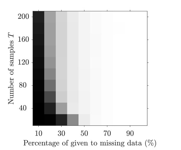
Figure 1: Transition diagram from failure to success when the data is missing randomly.

VI-B Matrix completion: comparison against nuclear norm heuristic

Following Corollary 3, we briefly discussed how one can use the results of this paper to solve a structured low-rank matrix completion problem. In this section, we compare the computational performance of our method against the nuclear norm heuristic. For the test system, we use the one in [22], which is a six-dimensional slightly damped autonomous discrete-time LTI system. A trajectory $w$ of length $T=500$ was generated by simulating the response of the system to random initial conditions sampled from $(U(0,1))^{6}$. For this example, a total of $276$ samples were periodically missing (with different periodicities). The goal of this example is to compare the computational performance of our proposed method (Algorithm 2) against the nuclear norm heuristic of [21] when solving the matrix completion problem.

Table I illustrates the results of matrix completion using the two approaches. The simulations were done on a standard Intel i7-10875H (2.30 GHz) machine with 16 GB of memory. Both approaches manage to solve the matrix completion problem up to numerical accuracy when only the first $200$ samples of $w^{-}$ were used. However, it is clear that the method proposed in Algorithm 2 is much faster than the nuclear norm minimization approach. When using the entire sequence of length $T=500$, the nuclear norm approach failed to return a result (due to insufficient memory). This is caused by the increasingly growing computations that are required to solve this problem. The complexity of the nuclear norm approach to structured low-rank approximation is not yet clear. However, it is known that complexity of this method to unstructured low-rank approximation is NP hard [26], which may explain the increased computational burden as in Table I. In contrast, the method proposed in Algorithm 2 successfully solves the problem with (fast) computation time even when the entire sequence was used.

TABLE I: Computational performance: matrix completion problem.

Compared values	Algorithm 2	Nuclear norm [21]
$T=200$ Time (s) Error	$\begin{matrix}0.0932\\ 6.3278\times 10^{-14}\end{matrix}$	$\begin{matrix}57.9953\\ 9.3051\times 10^{-9}\end{matrix}$
$T=500$ Time (s) Error	$\begin{matrix}0.2258\\ 6.1301\times 10^{-14}\end{matrix}$	$\begin{matrix}\textup{N/A}\\ \textup{N/A}\end{matrix}$

VII Discussion and Conclusions

In this paper, we investigated the problem of obtaining non-parametric data-based system representations from a set of irregularly measured data. For the general case of multi-input multi-output systems and random patterns of missing data, we improved an existing algorithm from the literature which now allows for computing the (not necessarily minimal) kernel representation of the system from irregularly measured data. Assuming that the system’s complexity is known, one can check if the output of the algorithm corresponds to the kernel representation upon running the algorithm.

If successful, we showed how one can use the output of the algorithm to obtain any complete finite-length behavior of the system by exploiting the properties of the Hankel matrix structure. This result has important properties, namely that the complete behavior of any length can be retrieved independent of the number of available (irregularly measured) values. For the case of periodically missing outputs with period $\ell+1$, we provided conditions on the input, such that any complete finite-length behavior of the system can be obtained.

The results of this paper can be further extended in several directions, for instance: (i) The guarantees provided in Section V considered the case where the output portion of the input/output data is missing. It was observed in simulations that our proposed methods work just as well when any $p$ instances of the data sample $w(t)$ were missing, whether it is the entire output portion or a combination of input and output portions. An interesting question for future research is how to impose conditions on the available inputs (rather than assuming availability of all inputs) such that guarantees similar to those in Section V can be shown. (ii) Studying other patterns of missing data, apart from periodically missing ones as in Section V is also an interesting problem for future work. Finally, investigating the effect of noise in the data on the proposed approach is an ongoing research work.

-A Proof of Theorem 4

$$\bar{Z}_{2} =\begin{bmatrix}z_{[1,p],0}^{(2)}&\cdots&\bar{\zeta}_{[1,p],\ell-1}^{(2)}&\bar{\zeta}_{[1,p],\ell}^{(2)}&I_{p}&z_{[1,p],\ell+1}^{(2)}\\ z_{[p+1,p(\ell+1)-n],0}^{(2)}&\cdots&\bar{\zeta}_{[p+1,p(\ell+1)-n],\ell-1}^{(2)}&\bar{\zeta}^{(2)}_{[p+1,p(\ell+1)-n],\ell}&\underline{\zeta}^{(2)}_{[p+1,p(\ell+1)-n],\ell}&z_{[p+1,p(\ell+1)-n],\ell+1}^{(2)}\end{bmatrix}.$$ (30)

$$\mathscr{Z}=\begin{bmatrix}Z_{1}\\ Z_{2}\end{bmatrix} =\scalebox{0.95}{$\begin{bmatrix}z_{[1,p(\ell+1)-n],0}^{(1)}&\cdots&\bar{\zeta}_{[1,p(\ell+1)-n],\ell-1}^{(1)}&\underline{\zeta}^{(1)}_{[1,p(\ell+1)-n],\ell-1}&\bar{\zeta}^{(1)}_{[1,p(\ell+1)-n],\ell}&0_{p(\ell+1)-n\times p}&z_{[1,p(\ell+1)-n],\ell+1}^{(1)}\\ \hline\cr z_{[1,p],0}^{(2)}&\cdots&\bar{\zeta}_{[1,p],\ell-1}^{(2)}&0_{p\times p}&\bar{\zeta}_{[1,p],\ell}^{(2)}&I_{p}&z_{[1,p],\ell+1}^{(2)}\\ z_{[p+1,p(\ell+1)-n],0}^{(2)}&\cdots&\bar{\zeta}_{[p+1,p(\ell+1)-n],\ell-1}^{(2)}&0_{p\ell-n\times p}&\bar{\zeta}^{(2)}_{[p+1,p(\ell+1)-n],\ell}&\underline{\zeta}^{(2)}_{[p+1,p(\ell+1)-n],\ell}&z_{[p+1,p(\ell+1)-n],\ell+1}^{(2)}\end{bmatrix}.$}$$ (31)

Notice that $\mathscr{Z}\in\mathbb{R}^{2p(\ell+1)-2n\times q(\ell+2)}$ has $2p(\ell+1)-2n\geq p(\ell+2)-n$ rows. Recall that if Algorithm 1 is successful with $d=\ell+2$, the kernel representation of the system would then be given by $p(\ell+2)-n$ linearly independent rows of $\mathscr{Z}$. Therefore, our goal now is to prove that rank$(\mathscr{Z})=\textup{dim}(\textup{ker}(\mathscr{H}^{\top}_{\ell+2}(w)))=p(\ell+2)-n$.

Consider again the matrix $\bar{H}_{2}$ (with the second to last block row expanded by partitioning $w$ appropriately)

$$\scalebox{0.9}{$\bar{H}_{2}=\begin{bmatrix}w(1)&w({\ell+2})&\cdots&w({(n_{c}-1)(\ell+1)+1})\\ w(2)&w({\ell+3})&\cdots&w({(n_{c}-1)(\ell+1)+2})\\ \vdots&\vdots&\vdots&\vdots\\ u({\ell})&u({2\ell+1})&\cdots&u({(n_{c}-1)(\ell+1)+\ell})\\ \begin{pmatrix}u({\ell+1})\\ y(\ell+1)\end{pmatrix}&\begin{pmatrix}u({2\ell+2})\\ y(2\ell+2)\end{pmatrix}&\cdots&\begin{pmatrix}u({n_{c}(\ell+1)})\\ y({n_{c}(\ell+1)})\end{pmatrix}\\ w(\ell+2)&w({2\ell+3})&\cdots&w({n_{c}(\ell+1)+1})\end{bmatrix}$},$$

and recall that rank$(\bar{H}_{2})=m(\ell+2)+n$ due to Lemma 3. If the block row $\begin{bmatrix}y(\ell+1)&y(2\ell+2)&\cdots&y({n_{c}(\ell+1)})\end{bmatrix}$ is removed from the above matrix, we obtain

where $\tilde{H}\in\mathbb{R}^{m(\ell+2)+p\ell\times n_{c}}$. Pre-multiplying by a square full rank permutation matrix $\tilde{\Pi}_{r}$, $\tilde{H}$ can be expressed as

where $X_{1}\coloneqq\begin{bmatrix}x(1)&x(\ell+2)&\cdots&x((n_{c}-1)(\ell+1)+1)\end{bmatrix}$ and the matrix $\mathscr{T}_{3}$ is square or has more rows than columns (since $p\ell\geq n$). Further, $\mathscr{T}_{3}$ has full column rank due to the identity on the upper left block and the full rank matrix on the lower right block (see Assumption 1). Following the same arguments as in Lemma 3, we find that rank$(\tilde{H})=m(\ell+2)+n=\textup{rank}(\bar{H}_{2})$.

This implies that the deleted block row, i.e., $\begin{bmatrix}y(\ell+1)&y(2\ell+2)&\cdots&y({n_{c}(\ell+1)})\end{bmatrix}$, can be expressed as a linear combination of the other rows of $\bar{H}_{2}$. In other words, we can always select $p$ rows in $\bar{Z}_{2}$ (without loss of generality, let them be the first $p$ rows) such that $\bar{Z}_{2}$ takes the form in (30) and satisfies $\bar{Z}_{2}\bar{H}_{2}=0$, where $z^{(2)}_{i,j}=\begin{bmatrix}\bar{\zeta}^{(2)}_{i,j}&\underline{\zeta}^{(2)}_{i,j}\end{bmatrix}$ and $\bar{\zeta}^{(2)}_{i,j}\in\mathbb{R}^{1\times m}$ while $\underline{\zeta}^{(2)}_{i,j}\in\mathbb{R}^{1\times p}$ (the same notation is used later for $\bar{Z}_{1}$ in (31)).

Since rank$(\bar{H}_{2})=\textup{rank}(\mathscr{H}_{\ell+2}(w))=m(\ell+2)+n$, $\bar{Z}_{2}$ can be extended by inserting zeros corresponding to the location of NaN entries in $H_{2}$ such that the matrix $\mathscr{Z}$ takes the form in (31) and satisfies $\mathscr{Z}\mathscr{H}_{\ell+2}(w)=0$ (see Lemma 1). Notice that $Z_{1}$ has full row rank, since $\bar{Z}_{1}$ has full row rank by definition of a basis for the left kernel of $\bar{H}_{1}$. Moreover, the first $p$ rows in $Z_{2}$ are linearly independent from the rows of $Z_{1}$, due to the location of the identity matrix $I_{p}$ in (31). Therefore, it holds that rank$(\mathscr{Z})=p(\ell+1)-n+p=p(\ell+2)-n$, which completes the proof.

Mohammad Alsalti received his B.Sc. in Mechanical Engineering from the University of Jordan, Jordan, in 2017. In 2017, he was an intern at NASA Ames Research Center as part of the intelligent robotics group. In 2020, Mohammad obtained his M.Sc. in Mechanical Engineering from the University of Maryland, College Park, USA. He is currently a Ph.D. student at the Institute of Automatic Control at Leibniz University Hannover, Germany. He is working on developing data-driven control techniques for linear and nonlinear systems.

Ivan Markovsky received the Ph.D. degree in electrical engineering from the Katholieke Universiteit Leuven, Leuven, Belgium, in February 2005. He is currently an ICREA Professor with the International Centre for Numerical Methods in Engineering, Barcelona. From 2006 to 2012, he was an Assistant Professor with the School of Electronics and Computer Science, University of Southampton, Southampton, U.K., and from 2012 to 2022, an Associate Professor with the Vrije Universiteit, Brussel, Belgium. His research interests are computational methods for system theory, identification, and data-driven control in the behavioral setting. Dr. Markovsky was the recipient of an ERC starting grant “Structured low-rank approximation: Theory, algorithms, and applications” 2010–2015, Householder Prize honorable mention 2008, and research mandate by the Vrije Universiteit Brussel research council 2012–2022.

Victor G. Lopez received his B.Sc. degree in Communications and Electronics Engineering from the Universidad Autonoma de Campeche, in Campeche, Mexico, in 2010, the M.Sc. degree in Electrical Engineering from the Research and Advanced Studies Center (Cinvestav), in Guadalajara, Mexico, in 2013, and his Ph.D. degree in Electrical Engineering from the University of Texas at Arlington, Texas, USA, in 2019. In 2015 Victor was a Lecturer at the Western Technological Institute of Superior Studies (ITESO) in Guadalajara, Mexico. From August 2019 to June 2020, he was a postdoctoral researcher at the University of Texas at Arlington Research Institute and an Adjunct Profesor in the Electrical Engineering department at UTA. Victor is currently a postdoctoral researcher at the Institute of Automatic Control, Leibniz University Hannover, in Hannover, Germany. His research interest include cyber-physical systems, reinforcement learning, game theory, distributed control and robust control.

Matthias Müller Matthias A. Müller received a Diploma degree in Engineering Cybernetics from the University of Stuttgart, Germany, an M.Sc. in Electrical and Computer Engineering from the University of Illinois at Urbana-Champaign, US (both in 2009), and a Ph.D. from the University of Stuttgart in 2014. Since 2019, he is director of the Institute of Automatic Control and full professor at the Leibniz University Hannover, Germany. His research interests include nonlinear control and estimation, model predictive control, and data- and learning-based control, with applications in different fields including biomedical engineering and robotics. He has received various awards for his work, including the 2015 EECI PhD award, the inaugural Brockett-Willems Outstanding Paper Award for the best paper published in Systems & Control Letters in the period 2014-2018, an ERC starting grant in 2020, and the IEEE CSS George S. Axelby Outstanding Paper Award 2022. He serves as an editor of the International Journal of Robust and Nonlinear Control and as a member of the Conference Editorial Board of the IEEE Control Systems Society.

References

- [1] W. T. Miller, R. S. Sutton, and P. J. Werbos, Neural networks for control. MIT press, 1995.
- [2] T. Beckers and S. Hirche, “Stability of Gaussian process state space models,” in 2016 European Control Conference (ECC), 2016, pp. 2275–2281.
- [3] J. C. Willems, “From time series to linear system—part I: Finite dimensional linear time invariant systems, part II: Exact modelling, part III: Approximate modelling.” Automatica, vol. 22, no. 5, pp. 561–580, 675–694, 87–115, 1986.
- [4] J. C. Willems, P. Rapisarda, I. Markovsky, and B. L. De Moor, “A note on persistency of excitation,” Systems & Control Letters, vol. 54, no. 4, pp. 325–329, 2005.
- [5] C. De Persis and P. Tesi, “Formulas for data-driven control: Stabilization, optimality, and robustness,” IEEE Transactions on Automatic Control, vol. 65, no. 3, pp. 909–924, 2020.
- [6] H. J. van Waarde, C. De Persis, M. K. Camlibel, and P. Tesi, “Willems’ fundamental lemma for state-space systems and its extension to multiple datasets,” IEEE Control Syst. Lett., vol. 4, no. 3, pp. 062–607, 2020.
- [7] J. Berberich and F. Allgöwer, “A trajectory-based framework for data-driven system analysis and control,” in 19th IEEE ECC, pp. 1365–1370.
- [8] G. Pan, R. Ou, and T. Faulwasser, “On a stochastic fundamental lemma and its use for data-driven optimal control,” IEEE Transactions on Automatic Control, pp. 1–16, 2022.
- [9] C. Verhoek, R. Tóth, S. Haesaert, and A. Koch, “Fundamental lemma for data-driven analysis of linear parameter-varying systems,” in 60th IEEE CDC, 2021, pp. 5040–5046.
- [10] J. G. Rueda-Escobedo and J. Schiffer, “Data-driven internal model control of second-order discrete volterra systems,” in 59th IEEE CDC, 2020, pp. 4572–4579.
- [11] M. Alsalti, V. G. Lopez, J. Berberich, F. Allgöwer, and M. A. Müller, “Data-based control of feedback linearizable systems,” IEEE Transactions on Automatic Control, pp. 1–8, 2023.
- [12] I. Markovsky and F. Dörfler, “Behavioral systems theory in data-driven analysis, signal processing, and control,” Ann. Rev. in Control, 2021.
- [13] B. Azimi-Sadjadi, “Stability of networked control systems in the presence of packet losses,” in 42nd IEEE International Conference on Decision and Control (IEEE Cat. No.03CH37475), vol. 1, 2003, pp. 676–681 Vol.1.
- [14] J. Berberich, J. W. Dietrich, R. Hoermann, and M. A. Müller, “Mathematical modeling of the pituitary–thyroid feedback loop: role of a tsh-t3-shunt and sensitivity analysis,” Frontiers in endocrinology, vol. 9, p. 91, 2018.
- [15] S. Wildhagen, J. Berberich, M. Hertneck, and F. Allgöwer, “Data-driven analysis and controller design for discrete-time systems under aperiodic sampling,” IEEE Transactions on Automatic Control, vol. 68, no. 6, pp. 3210–3225, 2023.
- [16] I. Markovsky and F. Dörfler, “Data-driven dynamic interpolation and approximation,” Automatica, vol. 135, p. 110008, 2022.
- [17] G. Heinig and K. Rost, Algebraic Methods for Toeplitz-like Matrices and Operators. Berlin, Boston: De Gruyter, 1984.
- [18] G. Heinig and P. Jankowski, “Kernel structure of block Hankel and Toeplitz matrices and partial realization,” Linear Algebra and its Applications, vol. 175, pp. 1–30, 1992.
- [19] R. Pintelon and J. Schoukens, “Frequency domain system identification with missing data,” in Proceedings of the 37th IEEE Conference on Decision and Control, vol. 1, 1998, pp. 701–705 vol.1.
- [20] I. Markovsky and K. Usevich, “Structured low-rank approximation with missing data,” SIAM Journal on Matrix Analysis and Applications, vol. 34, no. 2, pp. 814–830, 2013.
- [21] Z. Liu, A. Hansson, and L. Vandenberghe, “Nuclear norm system identification with missing inputs and outputs,” Systems & Control Letters, vol. 62, no. 8, pp. 605–612, 2013.
- [22] I. Markovsky, “Exact system identification with missing data,” in 52nd IEEE Conference on Decision and Control, 2013, pp. 151–155.
- [23] ——, “The most powerful unfalsified model for data with missing values,” Systems & Control Letters, vol. 95, pp. 53–61, 2016.
- [24] I. Markovsky and F. Dörfler, “Identifiability in the behavioral setting,” IEEE Transactions on Automatic Control, pp. 1–11, 2022.
- [25] I. Krauss, V. G. Lopez, and M. A. Müller, “Sample-based observability of linear discrete-time systems,” in 2022 IEEE 61st Conference on Decision and Control (CDC), 2022, pp. 4199–4205.
- [26] N. Gillis and F. Glineur, “Low-rank matrix approximation with weights or missing data is np-hard,” SIAM Journal on Matrix Analysis and Applications, vol. 32, no. 4, pp. 1149–1165, 2011.