A multi-modal representation of El Niño Southern Oscillation Diversity

Abstract

The El Niño-Southern Oscillation (ENSO) is characterized by alternating periods of warm (El Niño) and cold (La Niña) sea surface temperature anomalies (SSTA) in the equatorial Pacific. Although El Niño and La Niña are well-defined climate patterns, no two events are alike. To date, ENSO diversity has been described primarily in terms of the longitudinal location of peak SSTA, used to define a bimodal classification of events in Eastern Pacific (EP) and Central Pacific (CP) types. Here, we use low-dimensional representations of Pacific SSTAs to argue that binary categorical memberships are unsuitable to describe ENSO events. Using fuzzy unsupervised clustering, we recover the four known ENSO categories, along with a fifth category: an Extreme El Niño. We show that Extreme El Niños differ both in their intensity and temporal evolution from canonical EP El Niños. We also find that CP La Niñas, EP El Niños, and Extreme El Niños contribute the most to interdecadal ENSO variability.

Teaser Unsupervised fuzzy categorization of El Niño-Southern Oscillation reveals distinct onset dynamics of extreme El Niño events

1 Introduction

The El Niño-Southern Oscillation (ENSO), characterized by anomalous sea surface temperature (SST) in the tropical Pacific, exhibits notable diversity in its temporal evolution and spatial distribution of anomalies. The El Niño events of 1982-83 and 1997-98, for instance, recorded exceptionally high sea surface temperature anomaly (SSTA) values in the eastern equatorial Pacific, whereas the El Niño of 2002-03 were notably less extreme and primarily restricted to the central equatorial Pacific [28]. Despite each being categorized as an El Niño, the 2002-03 event exhibited global climate conditions distinct from those of the earlier two events. In order to describe these event-to-event differences, El Niño events have been categorized as Eastern Pacific (EP), and Central Pacific (CP) types [12]. EP El Niño events typically have their peak SSTA in the Eastern Pacific, exhibit stronger intensities, and a largely reduced zonal thermocline slope, resulting in the discharge of warm water from the equatorial thermocline. In contrast, CP events show peak SSTA in the Central Pacific and are comparatively weaker with more limited changes in zonal thermocline slope and reduced warm water discharge [23, 8]. Despite considerable research, the underlying causes of ENSO diversity remain elusive [25, 11, 12]. And while some general circulation models (GCMs) do exhibit ENSO event-to-event differences, their representation of ENSO diversity appears to be model dependent and is often different in intensity, pattern and duration than observed [7].

The different types of ENSO events have substantially different downstream impacts on the global climate and dynamics [39]. CP El Niño events, for instance, result in a more intense but abbreviated monsoon season over northwest Australia, as compared to their EP El Niño counterparts [42]. To move beyond studying individual events and establish more generalized statements on the remote impacts of different ENSO types, as well as to assess the representation of ENSO diversity in GCMs, various approaches have been proposed for grouping ENSO events in a quantitative manner. Most of these approaches involve the definition of one or two indices capturing the location of the highest SSTA in the tropical Pacific. These indices are obtained by averaging over specific regions or using Empirical Orthogonal Functions (EOFs) [2, 22, 23, 40]. Alternative indices based on outgoing longwave radiation [47] or statistical properties of tropical SSTA [46] have also been suggested. Classification of ENSO events is typically achieved by applying a threshold to these indices. For example, [23] identify events as EP-type when the DJF average of the Niño3 index (5°N-5°S, 150°W-90°W) exceeds 0.5 K and is larger than the Niño4 index (5°N-5°S, 160°E-150°W), whereas events are considered CP-type events when the DJF average of the Niño4 index is over 0.5 K and surpasses the Niño3 index DJF mean. However, variations in classification emerge depending on the chosen definitions. Comprehensive summaries and comparisons of these approaches can be found in [32, 50, 12].

More recently, clustering techniques have been used to identify distinct categories of ENSO events. For example, [27] utilized hierarchical clustering on SSTA and identified two classes associated with EP and CP events, characterized by distinct air-sea coupling strengths and dynamics. [45] applied K-means clustering to Hovmöller diagrams of El Niños and identified four different El Niño classes. Clustering approaches have also been employed by [16, 26, 3] on climate model outputs to assess biases in ENSO representation.

The prevailing assumption of these studies is that event-to-event differences can be classified discreetly into distinct types. However, [40] and others [7] demonstrate that the observed distribution of ENSO events in EOF space is rather continuous. This is supported by [13] who provides a more pertinent description of event distribution as a function of longitude, indicating a wider range of spatial patterns.[11] highlight that both EP- and CP-type events share common underlying dynamical processes, albeit with varying importance depending on the longitude. [43] attribute the longitudinal dependence to the shift in the Walker circulation in a simple theoretical framework. [30] argue that two initial patterns exist, which, under stochastic atmospheric forcing, amplify into EP and CP events or their combinations, thus resulting in a broad range of ENSO types.

Here, we build upon the idea that the observed distribution of ENSO events is continuous in low-dimensional representational spaces such as those based on EOFs, and contend that a binary ‘yes-no’ classification of the events is not compatible with observed variability. We thus propose to use a fuzzy clustering of the low dimensional representations to allow for non-binary event category memberships. In particular, we use a Gaussian Mixture Model (GMM) that approximates the data distribution as being composed of a sum of a finite number of Gaussian distributions, which represent the different event categories. Each data point can be assigned a posterior probability that quantifies its likelihood of belonging to each of the Gaussians.

These are the category memberships of the data point and they are inherently fuzzy and non-binary (i.e. they are probabilities between 0 and 1), which allows us to model ENSO events in terms of their likelihood of occurrence. Instead of asking if a given winter month belongs to a particular event category (answerable as a ‘yes’ or ‘no’), we ask how likely it is that the month could belong to the category. As a consequence, composite patterns of relevant climatic variables associated with the various ENSO types are estimated as weighted averages, with the weights being the categorical memberships.

An additional contribution of our work is that we conduct thorough sensitivity checks to ensure that the estimated ENSO event classification is robust. We show that our approach generalizes to non-linear transformations by using neural networks (NN) instead of EOFs to encode the data to a low dimensional representation. To further assess robustness, we analyze eight different reanalysis datasets, alter the dimensionality of our representation, and include sea surface height anomalies (SSHA) in addition to SSTA.

2 Results

2.1 ENSO diversity is well explained by five categories

Figure 1: Low dimensional representation of SSTA fitted by a GMM. SSTA of El Niño and La Niña events are projected onto EOF1 and EOF2. Their distribution is approximated by a GMM with 5 categories. The decodings of the Gaussian means are illustrated in panels (B-F)

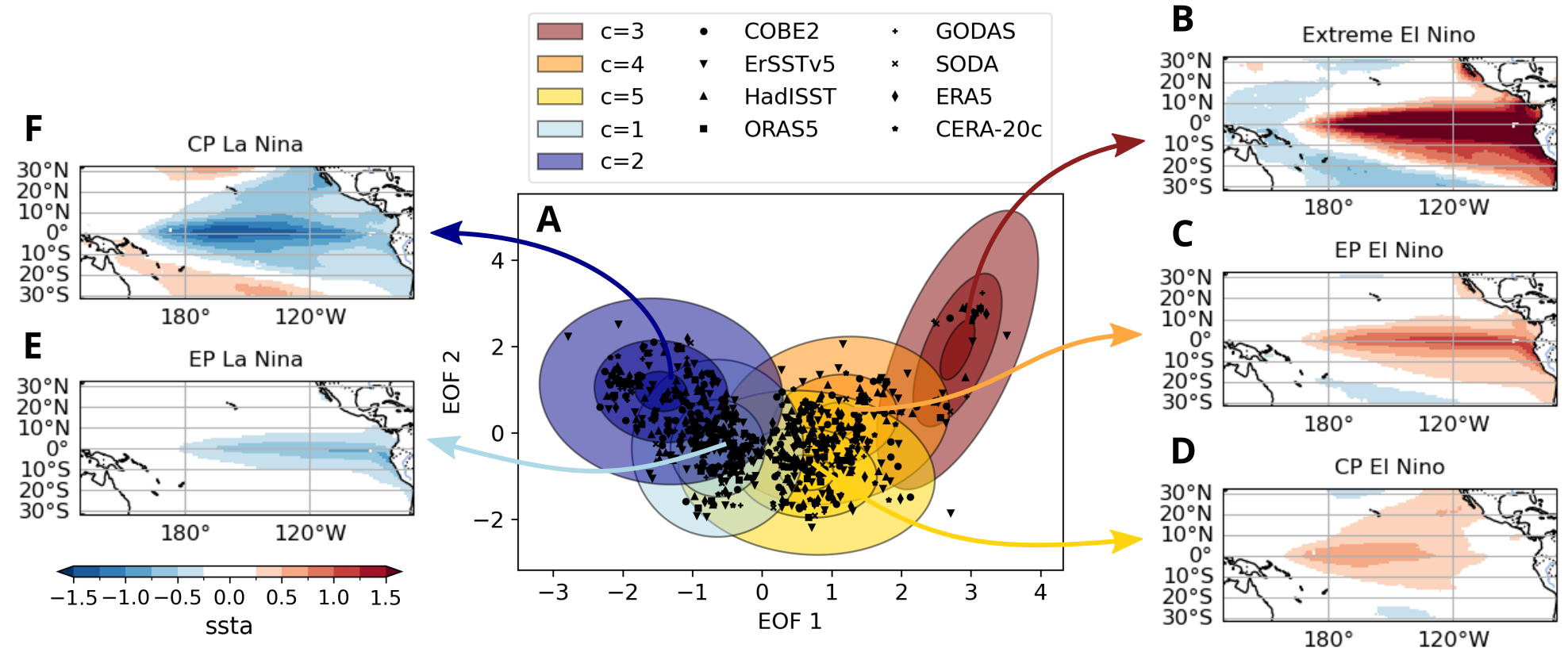
The two most dominant EOFs of all eight SSTA datasets combined (Sec. 4.1) resemble the well-known spatial patterns associated with the ENSO, i.e., EOF1 resembles the canonical ENSO pattern with anomalies in the central-eastern Pacific, while EOF2 exhibits an east-west dipole structure (Fig. S2). On projecting the average December-January-February SSTA pattern of all El Niño and La Niña events from the data on to the EOF1-EOF2 space, we find that the data distribution does not exhibit distinct clusters but rather forms a continuous, boomerang-like shape interspersed with regions of higher density (Fig. 1A). The boomerang-like shape has been reported in earlier EOF analyses of ENSO datasets and it encodes the nonlinear relationship between the dominant EOF modes, which is attributable to nonlinearities and asymmetries in ENSO dynamics [40, 7].

The nonlinear relationship itself can be accounted for by using a nonlinear transformation in place of the linear EOF-based transform, e.g., an autoencoder, and in that case, the boomerang-like shape is replaced by a simple linear relation between the two latent dimensions.

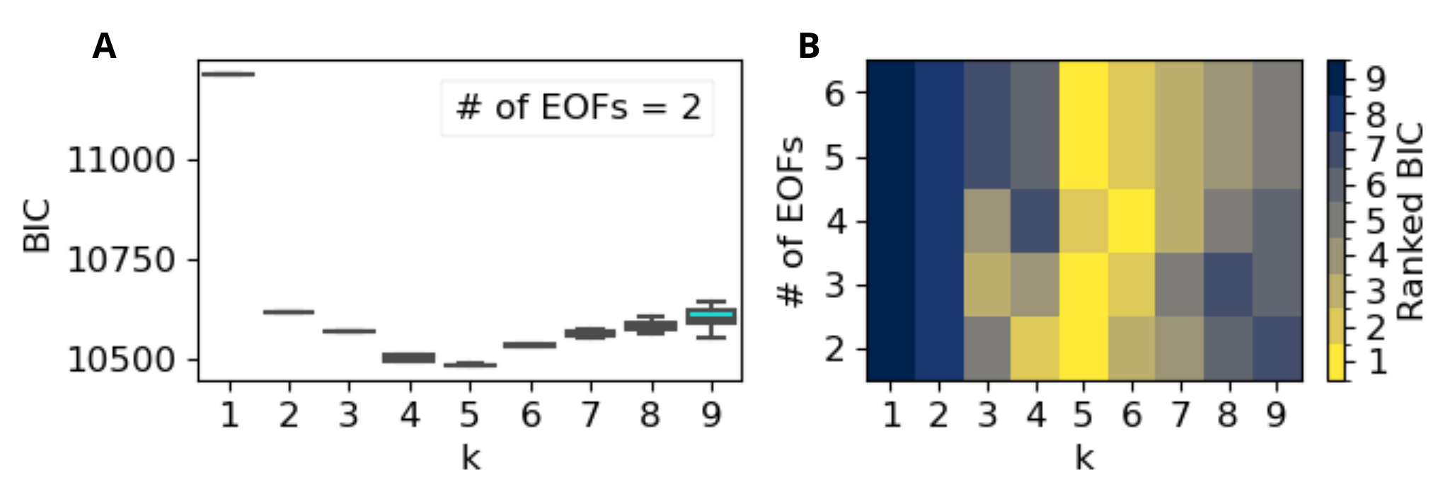
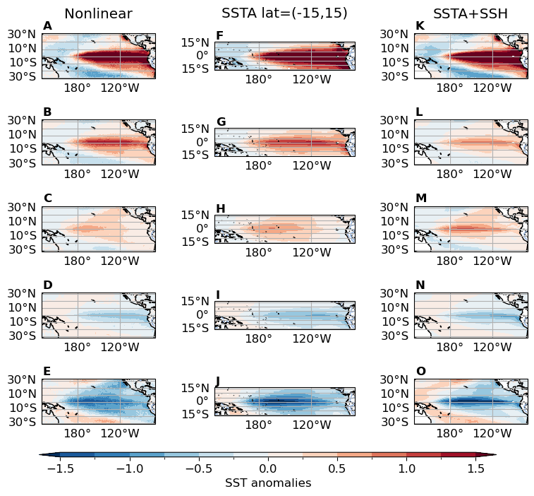
The data distribution in the EOF1-EOF2 space is modeled using a GMM with $k\ =\ 5$ components, which was determined using the Bayesian Information Criterion (BIC) to ensure parsimony (see Sec. A.2, 4.5, Fig. S3). The five Gaussians are arranged in a row along the boomerang from the coldest events at the leftmost tip to the warmest events at the rightmost end (Fig 1C). On examining the spatial SSTA patterns of the means of all five Gaussian, we find that three of the five Gaussians represent El Niño-like patterns (Fig. 1B-D), while the two remaining Gaussians encode La Niña-like patterns (Fig 1E-F). In fact, two of the three El Niño Gaussians correspond closely to the existing EP El Niño (Fig. 1B) and CP El Niño (Fig. 1C) categories, whereas the third, new category corresponds to extreme, basinwide warming, and is referred to here as the Extreme El Niño (discussed in more detail in Sec. 2.2). The two Gaussians representing La Niña diversity correspond clearly to the existing CP La Niña (Fig. 1F) and EP La Niña (Fig. 1E) categories. We find that the overall classification of the SSTA patterns into the five categories is fairly robust: changing the number of EOFs, incorporating SSHA data along with the SSTA, or varying the latitudinal range of the input all give us the same qualitative results (Fig. S4).

Figure 2: Probabilistic category membership. The conditional probability, $p\left(c_{k}|z(t)\right)$, that an event $z(t)$ belongs to the category $c_{k}$. Probabilities are averaged over the eight different datasets. The categories are sorted in the following order (top to bottom): Extreme El Niño, EP El Niño, CP El Niño, EP La Niña, and CP La Niña.

Figure 3: Probabilistic weighted composites of SSTA, SSHA, and OLR anomalies. We obtain weighted composites of SSTA, SSHA, and OLR anomalies for each category using Eq. 4. The composites of the CP El Niño, EP La Niña, and CP La Niña categories resemble similar patterns to classical indices-based composites (see Fig. S7). Separating Extreme El Niño and EP El Niño events, however, yields distinctly different patterns with a higher signal-to-noise ratio than conventional composites. The percentages noted in the subplot titles represent the proportion of statistically significant points relative to the total number of grid points. Significant regions are indicated by dotted areas above the 95th confidence interval.

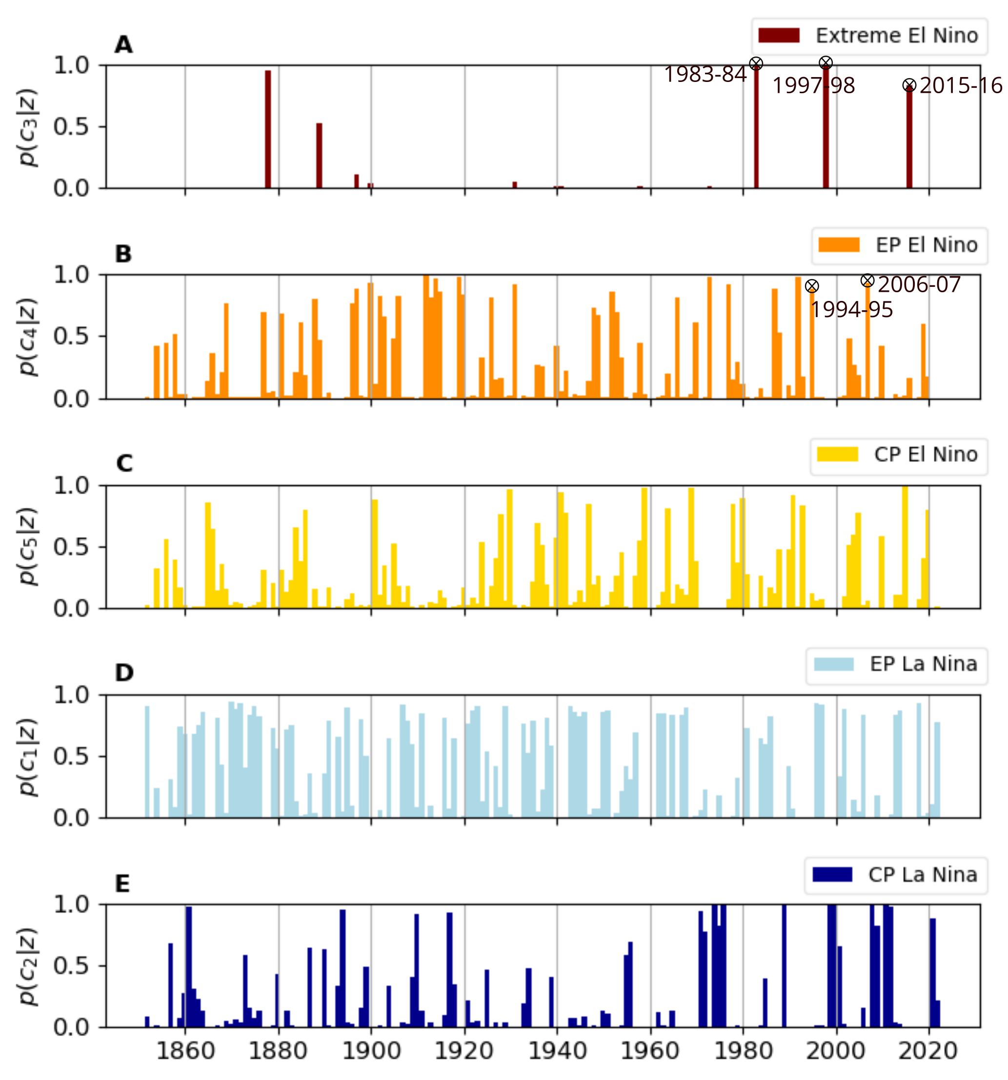
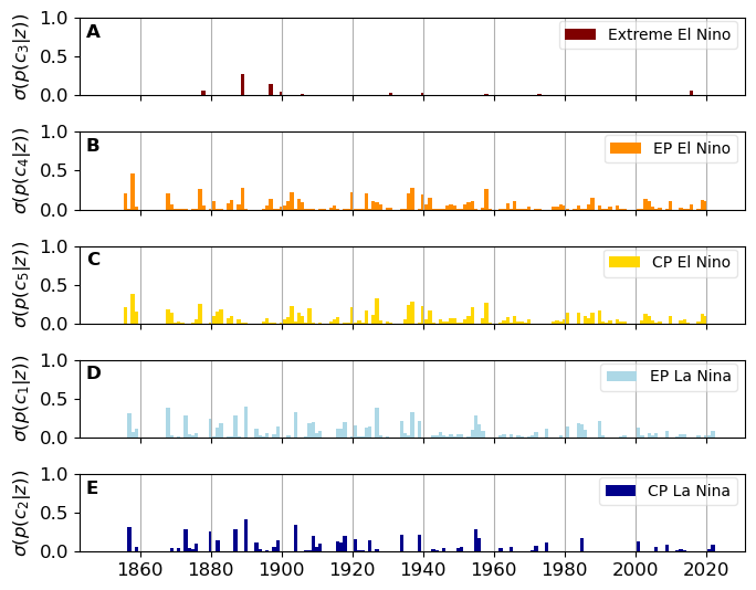
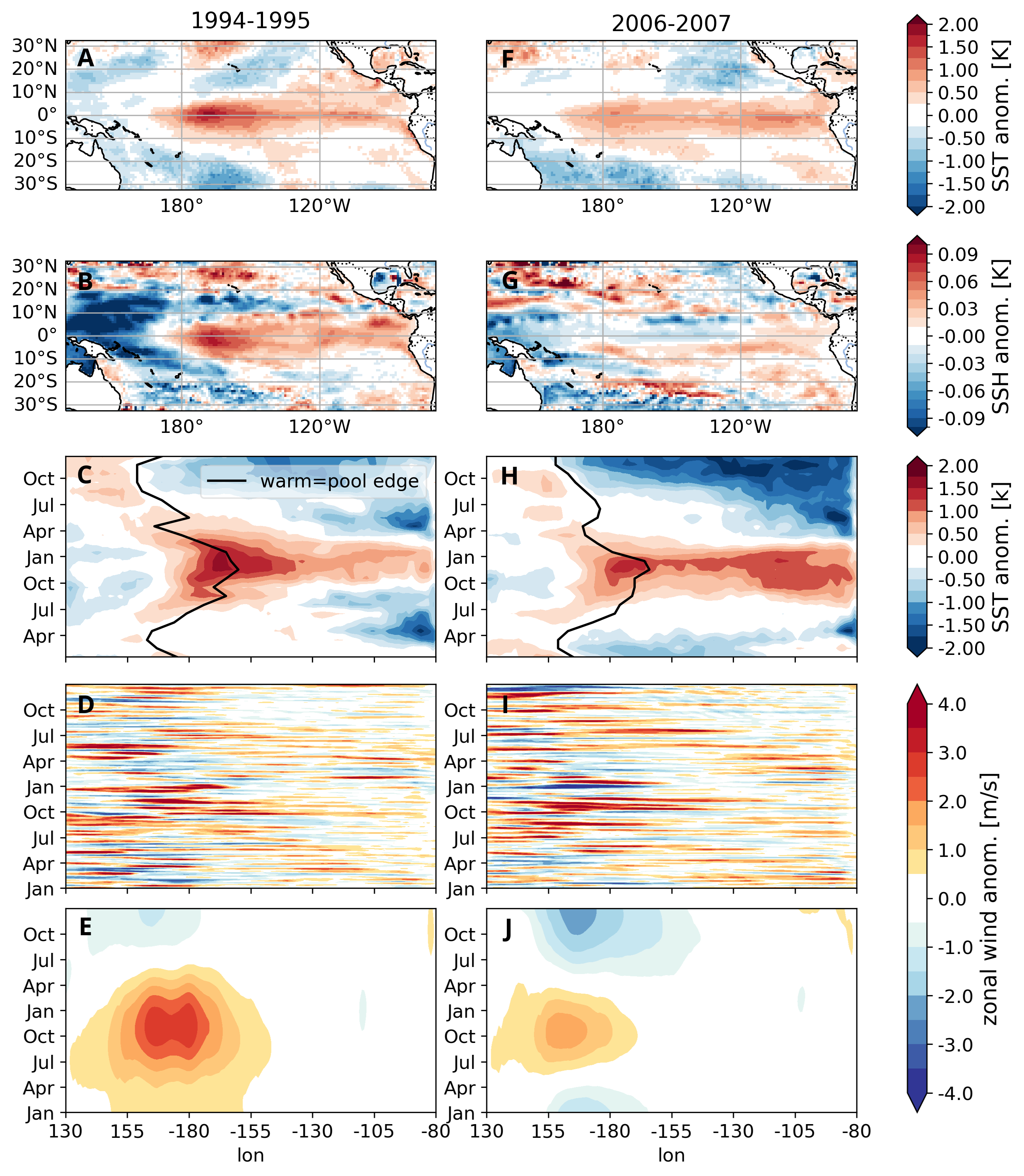
The GMM further enables us to estimate the likelihood $p\left(c_{k}|z(t)\right)$ that a chosen winter month $z(t)$ belongs to the category $c_{k}$ (Eq. 3), i.e. the category membership of that winter month. The category membership for each winter month averaged across the eight datasets result in five time series of probabilities - one for each category - which we interpret as indices of occurrence of the categories in the time period of analysis (Fig. 2). We find that the indices are not sensitive to the dataset used for their estimation, as seen in the relatively small spread of the membership probabilities over the eight datasets at each time point (Fig. S4). Comparing the category membership series for EP and CP El Niño events (Fig. 2B,C) to two existing classifications - the Niño3-Niño4 classification by [23] and the EOF-based E/C classification by [40] - we find that our classification is mostly in agreement with the earlier labels (Tab. S1). Differences, when they do occur, correspond to differences between the other classifications as well, and can thus be attributed to the lack of consistency in the older classifications themselves [50, 11, 32]. The two El Niño events of 1994-95 and 2006-07, however, are classified by both of the earlier classifications as CP events, whereas we find them to be EP events (Tab. S1). This is likely due to the fact that the warm water anomalies span from the Central to the Eastern Pacific during the duration of these events, leading to possible ambiguities in the event definition (Fig. S10). Notably, the 2006-07 event is referred to as double-peak El Niño due to two warm peaks of SSTA in the tropical Pacific [38].

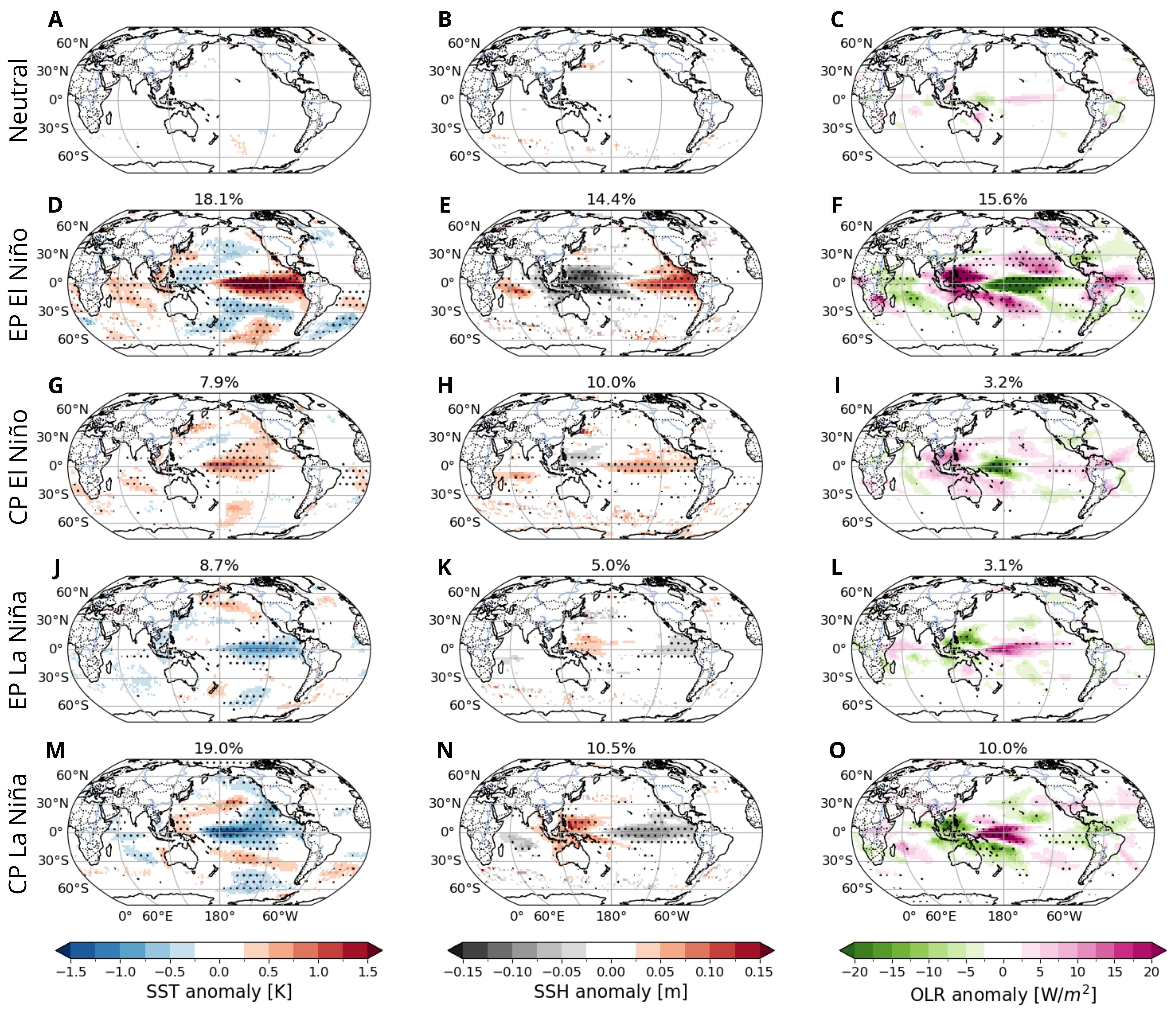
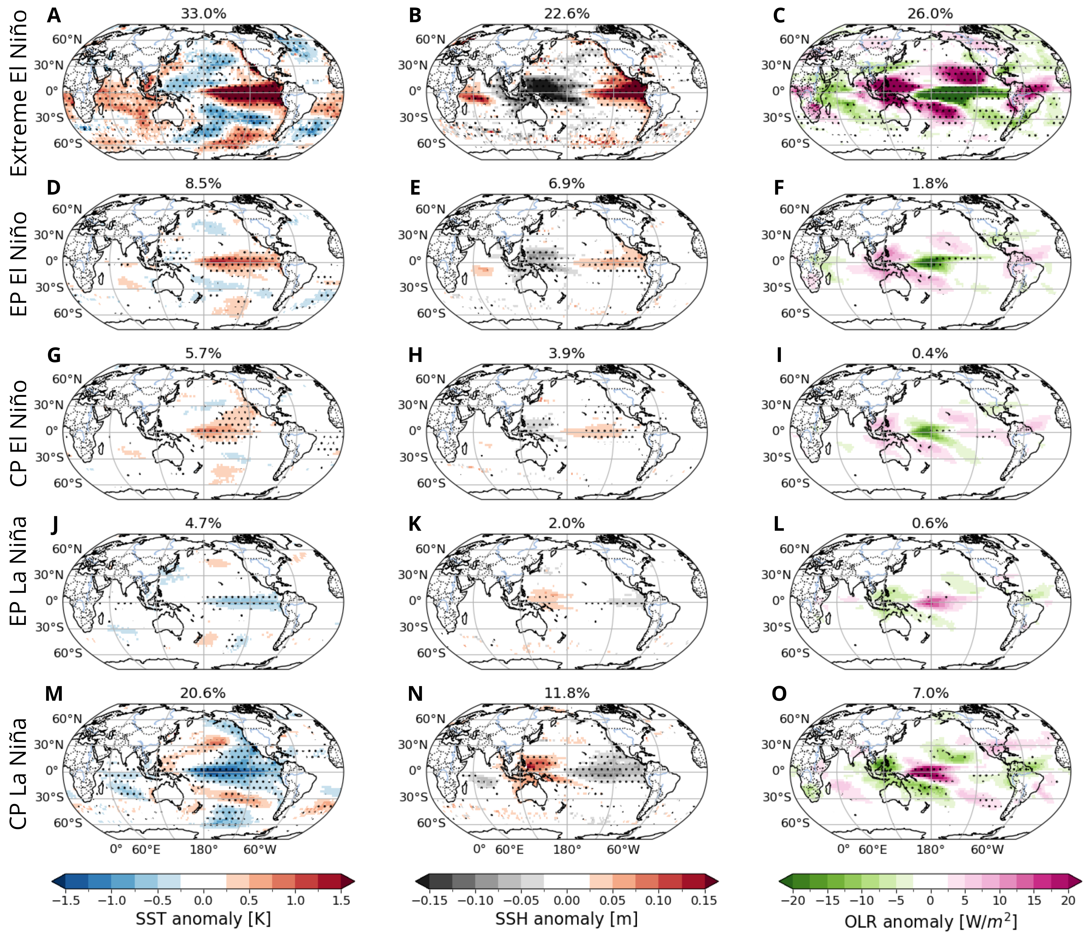
The correspondence between our classification and earlier methods is further exemplified by the similarities of variability patterns associated with the different categories. The average composite maps of the CP El Niño, EP La Niña, and CP La Niña categories obtained in this study (Fig. 3, third to fifth rows) exhibit similar patterns to the indices-based EP- and CP-type La Niña composite maps (Fig. S7, third to fifth rows). A subtle difference between the two sets of composite maps, however, is that the maps shown in Fig. 3 are obtained as weighted averages of the monthly data over the entire time period, where the weights are proportional to the category memberships (Eq. 4), whereas the composites in Fig. S7 are simply the average values of only labeled time points, i.e. events. A consequence of the weighted averaging, and of the probabilistic classification proposed in this study, is that the statistical significance of the composite variability patterns has to be determined by random sampling of time points, whereas in the earlier binary classifications, a pointwise $t$-test is applicable (Sec. 4.7).

A major difference of the ENSO categorisation proposed here from previous approaches is that the variability patterns associated with the Extreme El Niño (Fig. 3A-C) and EP El Niño categories (Fig. 3D-E) do not have a unique match in previous methods and, in fact, appear to be merged in composite maps associated with the ‘canonical’ EP-type El Niño (Fig. S7, second row). Our approach thus differentiates very strong EP El Niño events from moderately strong EP events, thereby creating the fifth category of ENSO events: the Extreme El Niño. We find that during Extreme El Niño events, statistically significant warmer-than-average SSTs occur in the Tropical Atlantic and Indian Oceans (Fig. 3A), which lack statistical significance for moderate EP El Niños. In general, by comparing the composite maps of the Extreme El Niño events (Fig. 3A-C) to those of the EP El Niño events (Fig. 3D-E), traces of the strong patterns seen for the Extreme El Niño are not statistically significant in the composites of the EP El Niño. This raises the question of whether the Extreme El Niño is different from the EP El Niño (in terms of its development and impact) sufficiently enough to merit its classification as a separate class of ENSO events. We address this point in Sec. 2.2.

2.2 Extreme El Niño events are different from EP El Niño events

Figure 4: Hovmoeller diagram of Extreme El Niño and EP El Niño category. Zonal averages of SSTA (A,B), SSHA (C,D), high-frequency zonal wind (HF, (H,F)), and low-frequency zonal wind (LF, (G,H)) anomalies are calculated from 5°S to 5°N for each month in the year preceding and succeeding an event. Averages for the Extreme El Niño (first column) and EP El Niño (second column) categories are performed, with each event weighted by their respective membership probability. Only values that statistically exceed the 95th confidence interval are displayed. Note that the color bar for the Extreme El Niño category spans a larger range than for the EP El Niño categories. The black line in (A) and (B) indicates the warm-pool edge, i.e., the 29°C SST isotherm, which captures the zonal shift of the Walker circulation.

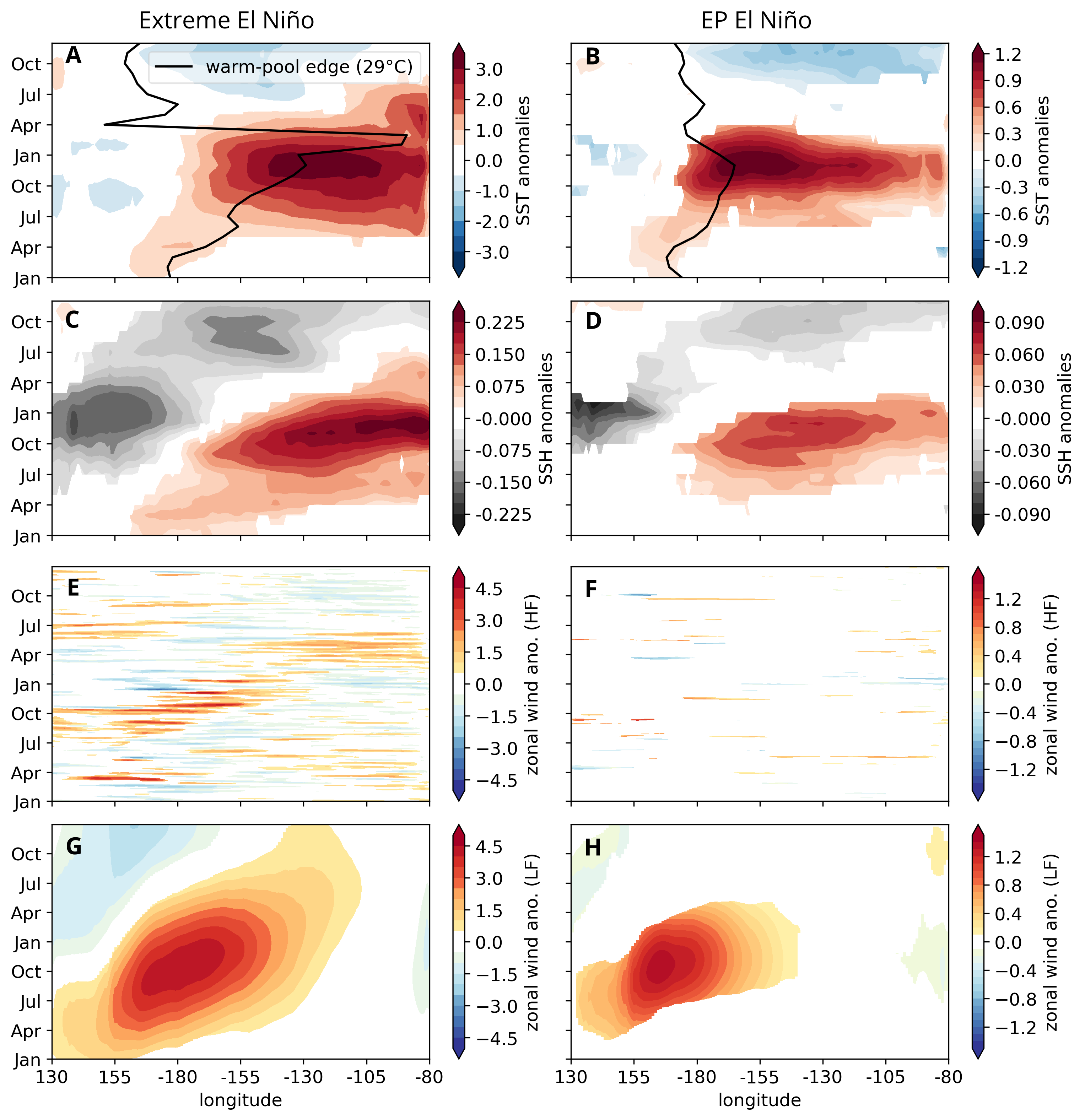
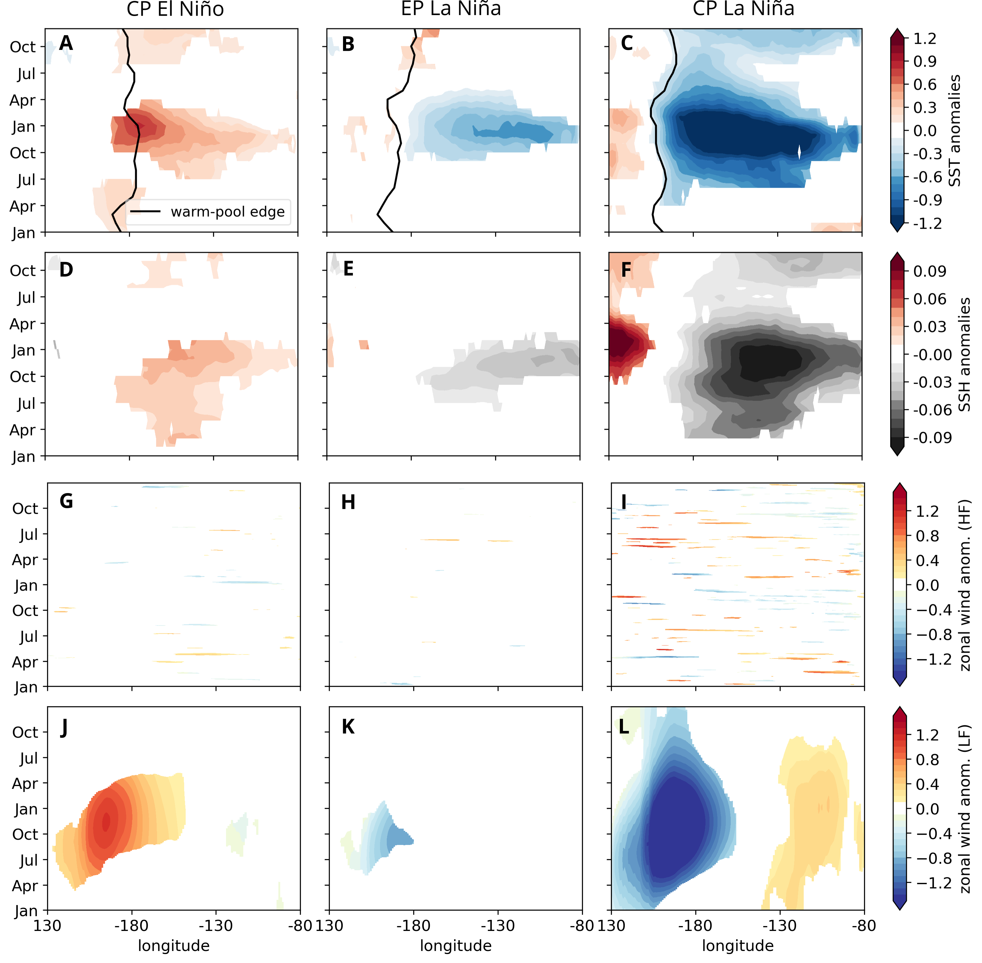
We estimate Hovmöller diagrams of Pacific SSTA and SSHA as well as high-frequency (HF) and low-frequency (LF) zonal wind components for each category, shown in Fig. 4 and Fig. S8. We separate zonal wind anomalies into HF (periods longer than 250 days) and LF (periods between 250 - 5 days) using Fourier filtering, as described by [10]. Meridional averages are performed from 5°S to 5°N for each month in the years preceding and succeeding an event. Weighted averages for each category were computed as described in Sec. 4.7. The black line in Fig. 4A-B indicates the warm-pool edge position, i.e., the longitude of the 29°C isotherm of SST along the equator, which captures the zonal shift of the Walker circulation (for further details see Sec. 4.9 and [43]. The warm-pool edge position for each category is again determined using weighted averages.

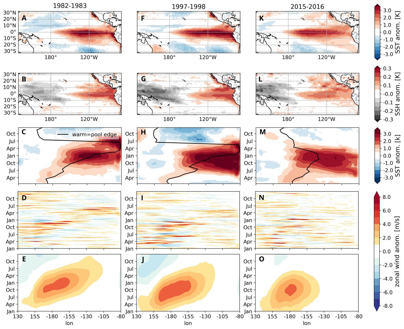
We find stronger SSTA and SSHA and an eastward-shifted SSTA peak in the Extreme El Niño category compared to the EP El Niño category which coincides with a further extended warm-pool edge (Fig. 4A-B). The maximum extent of the warm-pool edge occurs in the spring following the boreal winter of the El Niño peak, not coinciding with the maximum SSTA, a behavior not observed in EP El Niño composites. Aside from the greater SSTA and SSHA in the Extreme El Niño category, we also find significant differences in the onset phase of the two categories. The Extreme El Niño displays warm water volume anomalies, as described by SSHA, around the dateline already in the spring before an event, corresponding with a shift of the warm pool edge near the dateline and positive SSHA in that region (see Fig. 4C-D). EP El Niño events, on the other hand, do not demonstrate a consistent onset pattern in the preceding spring.

The HF zonal wind component (refer to Fig. 4E-F) is significantly positive to the west of the dateline during the developing phase of the Extreme El Niño category, a pattern not found in the EP El Niño category. Conversely, the LF zonal wind component manifests similarly in both categories, exhibiting positive anomalies during the spring onset although it does not extend as far East for EP El Niño events (Fig. 4G-H). The eastward propagation of both LF and HF components observed in the Extreme El Niño category suggests a coupling between the dynamics at the two time scales. Moreover, warm SSTA coincide with periods of positive LF components. For instance, LF winds that are stronger than average extend over the year preceding and following an Extreme El Niño event, mirroring the SSTA (see Fig. 4A,G), while for the EP El Niño category both the LF component and SSTA are only observed from the Aplril prior to the peak of the event to the following April (refer to Fig. 4B,H).

Our findings corroborate ideas presented in prior research on the impact of the Walker circulation's zonal shift and the influence of stochastic high frequency winds, called Westerly Wind Bursts (WWBs), on ENSO Diversity. [10] showed that the LF components of winds play an important role in the development of ENSO events. The modulation of intensity and type of El Niño events were attributed to WWBs in modeling studies by [15] and [33]. Notably, we observed consistent LF patterns (Fig. 4G,H) between the Extreme El Niño and EP El Niño categories, in contrast to the HF component.

[48] and others [43] have provided a mechanistic interpretation by using a simple stochastic dynamical ENSO model. The development of strong El Niño events is favored when the expansion of the warm pool across the Pacific coincides with a weak Walker circulation, providing favorable convective conditions for the development of WWBs which in turn can trigger strong El Niño events. [48] suggests that the intensity of the WWBs depends on the Madden Julian Oscillation (MJO). Work by [17] suggests that the state of the Indian Ocean may contribute to higher WWB activity and lead to super El Niño events.

Even though our categories are derived from DJF SSTA snapshots, our approach is still able to capture differences in the onset and development of the events in each category. This is indicative of the fact that the final SSTA patterns that are characteristic of each category are likely predetermined by distinctive mechanisms that are idiosyncratic to each category. Additionally, while highlighting the differences, it is important to emphasize once more that all categories are fuzzy, thus permitting to incorporate the broad spectrum of events. An example is the 2015/16 event depicted in Fig. S9, which shows a pattern situated somewhere between typical Extreme El Niño and EP El Niño categories, as indicated by their respective probabilities (0.83 for Extreme El Niño and 0.17 for EP El Niño). Our results support the findings presented by [35] and others [41, 19, 17] who proposed that strong El Niño events, such as those occurring in 1982/83 and 1997/98, constitute a distinctive regime of El Niños which is characterized by unique dynamics and more consistent and pronounced remote impacts. Our approach provides robust statistical evidence that this holds true in observed data.

2.3 Interdecadal ENSO variability is driven by EP and Extreme El Niño events

The membership probabilities of each category (Fig. 2) encodes a distinct pattern of decadal-to-multidecadal ENSO variability. In particular, the CP La Niña and the Extreme El Niño categories show a markedly prominent low-frequency variability, while the frequency of events within other categories appears to remain relatively constant. The apparently regular frequency of occurrence for CP El Niño events is in contrast to earlier findings, such as those from [25], who report an amplification in the frequency of CP events in the 21st century, driven by a shift in the SSTA variability in the tropical Pacific.

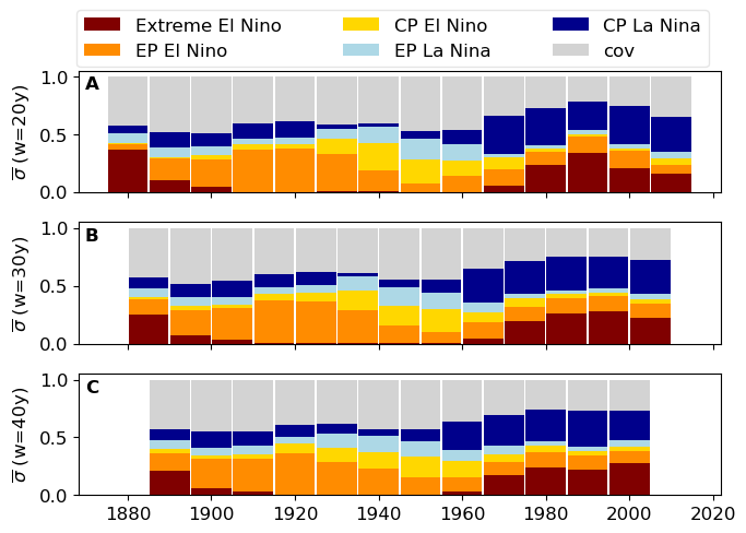
We quantify interdecadal ENSO variability by first decomposing the Niño3.4 index (derived from the HadISST dataset [34]) into contributions from each of the five ENSO categories (Eq. 5, Fig. 5A,B) and then estimating the relative contribution of each category (Fig. 5D, Eq. 6) to the overall Niño3.4 variance (Fig. 5C), evaluated over 30-year durations in steps of 10 years. Our results hold up against variations in window size (Fig. S11).

The total variance of the Niño3.4 index shows an increasing trend in the second half of the 20th century, which is in line with [9], who highlighted a shift in the mean and variance of Niño3 after the late 1970s, delineated as different El Niño regimes (dashed line in Fig. 5C). We find that while temporal changes are noticeable in the variance of all categories, only minor contributions to the total Niño3.4 variance are observed from the EP La Niña and CP El Niño categories (Fig. 4D). The CP La Niña category exhibits a significant contribution starting towards the end of the 20th century, and the EP El Niño category dominates the variance during the first decades of the 20th century. Meanwhile, the contribution of the Extreme El Niño category is particularly visible towards the end of the 19th and 20th centuries.

Figure 5: Contribution of each category to the temporal variability. The contribution of each category to the Niño3.4 index is obtained by Eq. 5, shown in (A). The distribution of Niño3.4 magnitude of each category (B) shows that the categories exhibit different SSTA amplitudes in the Tropical Pacific. The 30-year running standard deviation of Niño3.4 exhibits a multi-decadal variability (C). Especially, the combined Extreme El Niño and EP El Niño category variance (D) match the overall multi-decadal variability.

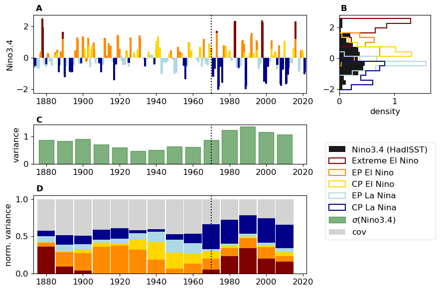
This result is consistent with recent work by [4], who identify strong eastern Pacific El Niño events as a key component influencing the decadal to multi-decadal variability of ENSO amplitude and asymmetry. However, our results provide a few additional novel insights into ENSO variability with respect to event diversity. We find that although the magnitude of total variance contributed by eastern Pacific warming events (i.e. Extreme El Niños and EP El Niños combined) since the turn of the 20th century is comparable to that seen during the period from 1880s to 1940s, the variance in the recent decades has been dominated mostly by Extreme El Niños with an approximately unchanged contribution from EP El Niños. This might be linked to the El Niño regime shift in the late 1970s [9] which was associated with a zonal reduction of the equatorial thermocline slope and a weakening of the easterlies, typically connected with strong El Niño events. Linked to the increased contributions from Extreme El Niños is the concurrent increase in the contributions of CP La Niñas since the 1970s (dark blue in Fig. 4D), manifest in very strong, multi-year events starting around 1970 (Fig. 4A). These results are consistent with a higher likelihood of stronger, central Pacific La Niñas following the heat discharge of strong El Niños, as exemplified by the 1998/99 La Niña event after the extreme 1997-98 El Niño [6].

We also find that during the ‘quiescent’ period of ENSO, roughly from the 1930s to the 1950s, most of the ENSO variability originated from central Pacific warming and eastern Pacific cooling events, which is consistent with the general idea that these event types are the ‘weaker’ kind of events, irrespective of whether we are dealing with warming or cooling. Particularly in the last two decades, the influence of central Pacific warming on the variance has been almost negligible. It is unclear however if the observed relations between quiescent ENSO and CP warming / EP cooling, and highly variable ENSO and EP warming / CP cooling will hold under future climate change. This might, however, be the focus of a future study, based on the representation of the reported categories in climate model ensembles.

3 Discussion

In this study, we have introduced a probabilistic framework to describe ENSO diversity, offering a continuous representation that overcomes the limitations of discrete classifications. Employing a Gaussian Mixture Model on the low-dimensional representation of a set of reanalysis products enabled us to address event-to-event differences as a superposition of fuzzy categories. Our findings support the notion that ENSO diversity should be conceptualized as a continuous phenomenon, characterized by certain states exhibiting higher probabilities throughout the observational period. Consequently, we advocate studying remote effects of ENSO diversity by weighting events by their category membership probabilities. We showed our results to be robust when tested against a variety of datasets, variables, and dimensionality reduction methods.

We found that El Niño events fall into three fuzzy categories, while La Niñas form two. Canonical EP-type El Niños were further subdivided in our classification between Extreme and EP El Niño categories, which not only varied in SSTA warming magnitudes but also displayed different onset dynamics. While a mechanistic explanation for the differences between Extreme El Niños and EP El Niños is not immediately available from an empirical study like ours, our findings are in line with previous studies based on global circulation models [15, 41, 33] as well as those based on stochastic dynamical models of intermediate complexity [44, 48]. These studies have attributed a weakened Walker circulation and favorable conditions for WWBs to the evolution of strong El Niño events which were also the defining points of difference between Extreme and EP El Niños in our results.

Our findings indicate that the Extreme El Niño category reveals statistically significant onset dynamics when compared to the EP El Niño category. This could potentially afford earlier predictability at lead times of 6-12 months for Extreme El Niño events relative to EP El Niño events, a prospect that warrants future research.

Furthermore, we have shown that strong El Niño events determine the low frequency variation in the tropical Pacific. These findings corroborate earlier work by [9] and [4] who attributed the shift of SSTA variance in the late 1970s to Pacific conditions favoring strong El Niño events. The CP La Niña category appeared to also contribute to the change in variance towards the end of the 20th century, a result not previously reported but consistent with results by [6] that strong La Niñas tend to follow strong El Niños.

We have also noted that in periods of low overall ENSO variability, contributions from CP warming / EP cooling events tend to dominate, whereas in periods of high ENSO variability (such as the last three decades), EP warming / CP cooling events contribute the most. In this context, it would be valuable to apply our approach to climate model output to compare the representation of ENSO diversity in these models relative to observed data. This would allow us to assess the model’s fidelity in capturing the full range of ENSO behavior, similar to the work of [13] and [3]. This comparative analysis would provide insights into the strengths and limitations of current climate models and guide future improvements in modeling ENSO dynamics.

4 Materials and Methods

4.1 Data

Our main analysis is conducted on monthly sea surface temperatures (SST) using eight reanalysis datasets. These include the

• NOAA Extended Reconstruction Sea Surface Temperature (ERSSTv5, $2{{}^{\circ}}\times 2{{}^{\circ}}$, 1854-2022) [51]

• ERA5 by Copernicus Climate Change Service ($0.25{{}^{\circ}}\times 0.25{{}^{\circ}}$, 1940-2022) [18]

• Global Sea Surface Temperature Data Sets (COBE-SST, $1{{}^{\circ}}\times 1{{}^{\circ}}$, 1891-2022) [20]

• Hadley Centre Sea Ice and Sea Surface Temperature data set (HadISST, $1{{}^{\circ}}\times 1{{}^{\circ}}$, 1870-2022) [34]

• Ocean Reanalysis System 5 (ORAS5,$0.25{{}^{\circ}}\times 0.25{{}^{\circ}}$, 1958-2022) [37]

• Simple Ocean Data Assimilation (SODA3.12, $0.25{{}^{\circ}}\times 0.25{{}^{\circ}}$, 1980-2022) [21]

• Global Ocean Data Assimilation System (GODAS, $0.33{{}^{\circ}}\times 1.0{{}^{\circ}}$, 1980-2022)[5]

• Coupled reanalysis of the twentieth century (CERA-20C, $1{{}^{\circ}}\times 1{{}^{\circ}}$, 1901-2009) [24]

For the multivariate analysis, we use SST and SSH which are only available in a subset of the aforementioned datasets, namely, in ORAS5, GODAS and CERA-20C. Anomalies are computed by linearly detrending the data after 1950 and removing the monthly climatology for each dataset. We select the Pacific region (130°E-70°W, 30°S-30°N) and interpolate each dataset to a $1{{}^{\circ}}\times 1{{}^{\circ}}$, resolution using the ’nearest-neighbor’ technique. The focus of our analysis is on El Niño and La Niña events. Therefore, we select boreal winter (December-January-February (DJF)) years where the DJF average SSTA in the Niño3.4 region are larger than 0.5 K or smaller than -0.5 K. Our results are consistent when defining events based on DJF exceeding the standard deviation.

The atmospheric variables used in this study, namely monthly OLR and the 6-hourly eastward component of the wind at 10 meters above the surface are taken from ERA5. Anomalies are computed as described above. We select the zonal wind component over the tropical Pacific (130°E - 70°W, 5°S-5°N) and decompose it into HF (periods longer than 250 days) and LF (periods between 250 - 5 days) using Fourier filtering, as described by [10].

4.2 Dimensionality reduction

In our approach, we model the multi-modal distribution of ENSO events using a mixture of Gaussians. Thereby, each Gaussian is a probabilistic cluster. Gridded geospatial fields have high dimensionality and are thereby generally sparsely distributed in space. Traditional clustering algorithms, like k-means, are based on a distance measure between data which becomes meaningless in high-dimensional spaces [31]. Thus, we reduce the degrees of freedom before clustering.

We denote the data by $X=\left(x\left(t_{1}\right),\ldots,x\left(t_{N}\right)\right)$ with a value of the field $x(t)$ at time $t=1,\ldots,N$ and grid point $s=1,\ldots,P$ denoted as $x_{s}(t)$. We reduce the dimensionality using a transformation $z(t)=e\left(x(t)\right)$ that maps $R^{P}\rightarrow R^{M}$ with $M<<P$. We call the lower dimensional representation latent space with $z(t)$ as the latent vector corresponding to the field $x(t)$ and the transformation encoder function, $e$. The inverse transformation from latent to data space is described by the function $\widehat{x}(t)=d\left(z(t)\right)$, called decoder. When reducing the dimensionality, we lose information such that $\widehat{x}\neq x$, i.e. the entire encoding-decoding pipeline can also be seen as a lossy compression-decompression method.

Figure 6: Sketch of the experimental setup. We transform the high-dimensional input fields to a low-dimensional latent space which is denoted by the encoder and decoder. The distribution of the data in the latent space is then approximated by a Gaussian mixture model.

4.3 Empirical Orthogonal Function Analysis

In this study, we use linear and non-linear dimensionality reduction techniques. Empirical Orthogonal Function (EOF) analysis (or Principal component analysis (PCA)) is a well-established linear dimensionality reduction technique for spatial-temporal data. The principal components correspond to the latent vector $z(t)\in R^{M}$ with its $r$ component at time $t$ is given by the linear transformation $z_{r}(t)=x_{s}(t)u_{rs}$. Here, $u_{r}\in R^{P}$ is the EOF and corresponds to the $r$th eigenvector of $\langle XX^{T}\rangle$ with the corresponding eigenvalue $\lambda_{r}$. As always, $r=1,\ldots,M$ is sorted by the eigenvalues such that the first eigenvector describes the most variance in the data. The inverse transformation is given by $x(t)=\lambda_{r}z_{r}(t)u_{r}$. We obtain the principal components for multiple datasets by concatenating the datasets along the time dimension. This way our principal components capture not only the variance of the data but also the variance between the datasets. In the multivariate case, we concatenate the different variables, i.e. $x(t)=\left(x_{SSTA}(t),x_{SSHA}(t),\ldots\right)$.

4.4 Autoencoder

  We use an autoencoder neural network to obtain a non-linear dimensionality reduction. We use convolutional neural networks for the encoder $e_{\phi}$ and decoder $d_{\theta}$ functions, respectively, where $\phi,\theta$ are the parameters of the network. The encoder takes as input the gridded data $x(t)$ and maps them to the lower dimensional latent vector $z(t)$, while the decoder maps $z(t)$ back to the data space $\widehat{x}(t)$. The encoder and decoder neural networks are trained to reduce information loss by the bottleneck. We use a mean-square error function to train the parameters of the autoencoder, i.e.

$$\text{argmin}_{\phi,\theta}\frac{1}{N}\left(\widehat{x}(t)-x(t)\right)^{2}.$$ (1)

Our encoder network consists of four convolutional layers followed by a linear layer. Each convolutional layer halves the x and y dimension of the input by using a kernel size of 3, a stride of 2, and padding of zero. The output of each convolutional layer is transformed by a ReLU function [1]. We double the number of channels in the first two layers and keep it fixed for the last two layers. After the last convolutional layer, we flatten the output and pass it through a linear layer whose output has the dimensionality $M$. The decoder is designed to be symmetric to the encoder. A linear layer is followed by four deconvolutional layers with each layer doubling the dimension of x and y. The number of channels are fixed in the first two convolutional layers but halve in the last two layers respectively. This way the output dimensionality matches the dimension of the encoder input, $x(t)$. Again we use the ReLU activation function after each layer except the last one. Different variables (SSTA, SSHA, …) are stacked in the channel dimension.

4.5 Gaussian mixture model

We use an unsupervised clustering approach to identify different types of ENSO events in the low-dimensional latent space from EOF and the AE. In the last decades, a variety of different unsupervised clustering methods have been developed (e.g. (Bishop, 2006)). Here, we use a Gaussian mixture model (GMM) to analyze the structure in the latent space. The advantage of GMM is that it is a probabilistic clustering approach where each cluster is described by a multivariate Gaussian distribution. The clusters can have overlapping probabilities and are thereby referred to as “fuzzy”. The fuzzy clusters should describe the distribution of ENSO diversity more realistically due to inherent noise in the climate system. Meanwhile, the probabilistic approach allows us to test how distinctly different the types of ENSO and their occurrence are. Mathematically, GMM assumes that the probability distribution of the latent space $p(Z)$ is generated by a mixture of Gaussians, i.e.

$$p(z)=p\left(c_{k}\right)p\left(z|c_{k}\right)=\pi_{k}N\left(z\mid\mu_{k},\Sigma_{k}\right),$$ (2)

where $K$ is the number of Gaussians with mean $\mu_{k}$ and covariance $\Sigma_{k}$ each. The probability of each Gaussian is denoted as $p\left(c_{k}\right)=\pi_{k}$ with $\pi_{k}=1$. The advantage of this approach is that we can estimate the probability of each event belonging to each cluster $p\left(z(t)|c_{k}\right)=N\left(z\mid\mu_{k},\Sigma_{k}\right)$. The parameters of the Gaussians $\mu_{k},\Sigma_{k}$ are estimated iteratively using the Expectation Maximization (EM) algorithm [49]. A detailed description of the EM algorithm for estimating GMM parameters can be found for instance in Murphy [29].

In order to estimate the optimal number of clusters $k$, we apply the Bayesian Information Criterion (BIC) [36]. The likelihood of the GMM can generally be increased using more clusters which on the other hand increases the complexity of the model and is therefore prone to overfitting. BIC is a model selection criterion that when minimized balances the model complexity to the increase in the likelihood. BIC is defined as $BIC(k)=Pln(N)-2ln\left(p\left(Z|\psi\right)\right)$ with $P$ is the number of parameters of the GMM, $\psi=\left(\pi_{k},\mu_{k},\Sigma_{k}\right)$, $N$ is the number of datapoints and $p\left(X|\psi\right)$ is the likelihood. In our analysis, we fit 100 GMMs with random initialization for each value of $k$ (number of Gaussians) and compute the BIC. The model with the lowest BIC represents the best trade-off between model complexity and fit quality. Additionally, the spread of the BIC values across different initializations serves as a measure of the robustness of the fit, indicating whether the Gaussian parameters consistently converge to the same values regardless of initialization.

We, thus, approximate the distribution of ENSO events by first transforming them into the lower dimensional latent space and then fitting a mixture of Gaussians in the latent space. This can be expressed as the following generative process, i.e. $p(x)\approx p\left(x|z\right)p\left(z|k\right)$. The transformation functions described above (PCA, Autoencoder) are technically the maximum a posteriori estimates of the generative distribution $p\left(x|z\right)$. The full generative model is described by Jiang et al. (Jiang et al., 2017) and allows a joint optimization of the GMM and the transformation function. For the sake of complexity and reproducibility, we focus on the model described above. A comparison to the full generative model did not show qualitative differences.

4.6 Category membership

The GMM approximation of the low-dimensional distribution enables us to assign conditional probabilities that an event $z(t)$ belonging to category $c_{k}$, using Bayes’ theorem:

$$p\left(c_{k}|z(t)\right)=\frac{p\left(c_{k}\right)p\left(z(t)|c_{k}\right)}{p\left(c_{k}\right)p(z(t)|p\left(c_{k}\right)}=\frac{\pi_{k}N\left(z(t);\mu_{k},\Sigma_{k}\right)}{\pi_{k}N(z(t);\mu_{k},\Sigma_{k}}.$$ (3)

These category membership probabilities, denoted as $p\left(c_{k}|z(t)\right)$, form a time series for each category, indicating the likelihood of occurrence. Notably, the conditional probabilities for a given event $z(t)$ across the categories sum up to one, i.e. $p\left(c_{k}|z(t)\right)=1$. This indicates that $p\left(c_{k}|z(t)\right)=1$ signifies the event belonging exclusively to category $c_{k}$. Conversely, events with probabilities shared among multiple categories cannot be assigned to a single category but exhibit some probability of belonging to two or more categories.

While we refer to these Gaussians as categories throughout our work, they primarily describe characteristics of regions with higher density within a continuous distribution, rather than distinctly different entities.

4.7 Probabilistic weighted averages

The effects of ENSO are typically assessed by examining the averages of a variable of interest under certain Pacific background conditions. For instance, to study how El Niño events impact precipitation, years in which the tropical Pacific SSTA exceed 0.5 K are selected, and an average of precipitation is calculated for those years. In our approach, we advise determining composites for each category $c_{k}$ of a desired variable, $y$, through their weighted average:

$$\overline{y}_{k}=p\left(c_{k}|z(t)\right)y(t),$$ (4)

where the weights are the conditional probabilities $p\left(c_{k}|z(t)\right)$ given for each event $t=1,\ldots,N$.

To examine the statistical relevance of the weighted mean ${\overline{y}}_{k}$, we compare ${\overline{y}}_{k}$ to the mean values of samples drawn randomly over the entire time period. In other words, we set our null hypothesis as ${\overline{y}}_{k}$ being an average derived from randomly drawn samples. To this end, averages are calculated from randomly sampled years and their respective means are computed. We then determine the p-values of ${\overline{y}}_{k}$ in relation to this distribution. Additionally, to account for multiple testing, we applied Dunnett’s test [14] for appropriate corrections.

4.8 Temporal variability

In order to study the contribution of the probabilistic categories to the temporal variability of a desired variable $y$, we can write the variable at time $t$ as

$$y(t)=p\left(c_{k}|z(t)\right)\cdot y(t)\ :=y_{k}(t),$$ (5)

where $y_{k}(t)$ represents the contribution of category $c_{k}$ to the variable $y(t)$.

The contribution of different ENSO categories to the temporal variance of $y$ is thus given by

$$\langle y^{2}\rangle=\langle\left(y_{k}\right)^{2}\rangle=\langle y_{k}^{2}\rangle+\frac{1}{2}\langle y_{l},y_{m}\rangle,$$ (6)

where the sum of cross-covariance-terms $\langle y_{l},y_{m}\rangle$ are denoted by $cov$.

4.9 Warm-pool edge

[43] propose that the diversity in ENSO is linked to the zonal shift of the Walker circulation over the Tropical Pacific. They suggest that the edge of the warm-pool serves as an indicator for deep convection shifts, characterizing it as the 29°C isotherm where SSTs saturate over the warm pool. The warm-pool edge is identified as the earliest longitude moving from 80°W (East) to 120°E (West), where the equatorial SST exceeds 29°C for a subsequent 10° westward.

Supplementary Materials

Appendix A Supplementary Text

A.1 Category membership

In order to compare our category membership with conventional index-based classifications of El Niño events, we present a comparison between the Niño3-Niño4 classification by [23], the EOF-based E/C classification by [40], and our category membership (Tab. S1).

The events 1983/84, 1997/98, and 2015/16 have a high membership probability in the Extreme El Niño category, while they are classified as EP-type events in the conventional methods. The 1951/52, 1972/73, 1976/77, and 1986/87 events show a high likelihood of being part of the EP El Niño category which concurs with conventional classifications. We identified the events of 1958/59, 1968/69, 1969/70, 1977/78, 1979/80, 2004/05, 2014/15, and 2019/20 as having a high probability of belonging to the CP El Niño category, also aligning with conventional classification.

We observe inconsistencies in indices-based classifications for the 1994/95 and 2006/07 events, displaying high membership probability for the EP El Niño category, despite being labeled as CP-type by Niño3-Niño4 and E/C definitions. The conventional EP- and CP-type definitions, however, lack consistency as summarized by [32, 50, 12].

A.2 Robustness

To assess the robustness of our approach, we conduct a sensitivity analysis by varying the number of EOFs. We perform the analysis for 2-6 EOFs and visualized the BIC as a function of categories in Fig. S3B. Since the BIC values exhibit changes with an increasing number of EOFs, we sort the mean BIC values for each number of EOFs and plotted their ranks. Our results consistently indicated that the 5-dimensional latent space yielded the lowest BIC values, except in the case of the 4-dimensional latent space, where the minimum BIC was observed at $k=6$. It is worth noting that the BIC values displayed a wider distribution at $k=6$ compared to $k=5$ in the 4-dimensional latent space which explains the deviation (not shown). Regardless of the number of EOFs, the mean encodings at $k=5$ exhibited consistent patterns akin to those observed in Fig. 1.

To assess the robustness of our categories with respect to the data employed, we repeated our analysis on input fields that were constrained within the range of 15°S - 15°N, effectively eliminating the influence of the subtropics. The encodings of GMM means for these restricted input fields are presented in Fig. S5F-J. Furthermore, we extended our analysis by incorporating SSHA as an indicator of oceanic conditions. For this purpose, we utilized reanalysis products (SODA, GODAS, ORAS5, and CERA-20C) that provide SSH data. The mean encodings of the optimal GMM incorporating SSHA are depicted in Fig. S5K-O. By comparing the mean encodings in Fig. S5, we qualitatively observe consistent patterns, aligning with the findings described in Sec. 2.2. Hence, our results exhibit robustness concerning both the geographical region within the tropical Pacific and the inclusion of additional variables in our analysis.

To examine the potential bias introduced by linear dimensionality reduction in our approach, we adopt an alternative method using a convolutional autoencoder. Unlike the EOF-truncation, this approach allowed for nonlinear dimensionality reduction of the SSTA fields. Here, we employ a symmetric autoencoder as described in Sec. 4.4. Subsequently, the GMM was fitted based on the low-dimensional representation obtained from the autoencoder.

The encodings of the optimal GMM means (Fig. S5A-E) exhibited similar patterns to those obtained from the EOF analysis. These results imply that a linear decomposition of the SSTA fields suffices to capture their diversity, minimizing concerns regarding bias introduced by the linear dimensionality reduction.

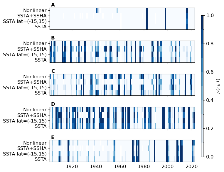
While we observe qualitative similarities in the obtained categories, there are slight variations in the conditional probabilities over time. Fig. S6 displays the conditional probabilities for each category across the different robustness tests described above. Although there are differences in events with low probabilities, events with high probabilities remain consistent.

Table S1: Classification of El Niño events. Listed are two commonly used indices-based classification approaches of El Niño events as well as our probabilistic clustering. We use E to denote Eastern Pacific, C for Central Pacific, and E^∗ for Extreme El Niño events. The Niño3-Niño4 approach by Kug et al. (2009) classifies events as E when the DJF average Niño3 > Niño4 and C when Niño4 < Niño3. Takahashi et al. (2011) uses the first two principal components of SSTA to create and E- and C-index. When DJF average E-index / C-index events are considered of type E and events are of type C when C-index / E-index. The last column shows the largest category membership and their probability in brackets, $p\left(c|x\right)$. In cases where the probabilities are shared (i.e. $0.4<p\left(c|x\right)<0.6$), we show the largest two category memberships. The blank entries denote cases in which the respective conditions were not met to classify an event.

	Niño3-Niño4	E/C	$p(c_{k}|x)$
1951-1952	E	E	E (0.87)
1953-1954	C		C (0.45) / E (0.33)
1957-1958	E	C	C (0.54) / E (0.44)
1958-1959	C		C (0.97)
1963-1964	E	C	C (0.80)
1965-1966	E	C	E (0.81)
1968-1969	C	C	C (0.97)
1969-1970	C		E (0.60) / C (0.37)
1972-1973	E	E	E (0.98)
1976-1977	E		E (0.92)
1977-1978	C		C (0.84)
1979-1980	C		C (0.89)
1982-1983	E	E	E*(1.00)
1986-1987	E	E	E (0.88)
1987-1988	C	C	E (0.52) / C (0.47)
1991-1992	E	C	E (0.99)
1994-1995	C	C	E (0.89)
1997-1998	E	E	E*(1.00)
2002-2003	C	C	C (0.51) / E (0.49)
2004-2005	C	C	C (0.77)
2006-2007	C	C	E (0.93)
2009-2010	C	C	C (0.58) / E (0.42)
2014-2015	C		C (0.98)
2015-2016	E	C	E*(0.83)
2018-2019	C	C	E (0.59) / C (0.40)
2019-2020	C	C	C (0.79)

  

Figure S2: EOF across all eight datasets. First (A) and second (B) EOFs obtained from all eight reanalysis datasets. The patterns resemble the typical ENSO tongue in the first EOF and the dipole structure in the second EOF.

  

Figure S3: Determining the optimal number of clusters. The distribution of BIC is computed for each number of clusters $k$ by fitting 100 GMMs which are randomly initialized. The mean, 10th and 90th percentile as well as the median are shown as boxplots for the two-dimensional EOF latent representation of SSTA (A). The same analysis is repeated by increasing the number of EOFs (B). The mean BIC over the 100 GMMs for each $k$ is ranked for each number of EOF to show that our results are robust with the number of EOFs used.

  

Figure S4: Variation of category membership. The conditional probability of an event $z(t)$ to belong to cluster $k$ has been averaged over the different datasets. The standard deviation between the different datasets is shown for each category.

  

Figure S5: Robustness of categories. A range of robustness tests unveils consistent patterns in the GMM decoded means. The initial column presents outcomes from employing a convolutional autoencoder for nonlinear dimensionality reduction. The subsequent column reveals the results obtained from a confined latitude range (15°S - 15°N) of the input data. The final column depicts the outcomes achieved when SSH anomalies are incorporated into our analysis. The categories are sorted in the following order (top to bottom): Extreme El Niño, EP El Niño, CP El Niño, EP La Niña, and CP La Niña

  

Figure S6: Robustness of category memberships. While the GMM categories maintain qualitative similarity amidst variations in our approach, the membership probabilities of each ENSO event within these categories do differ. The variations are represented as follows: The Nonlinear label signifies the use of a convolutional autoencoder for nonlinear dimensionality reduction. The term SSTA+SSHA identifies results incorporating SSHA. The label SSTA lat=(-15,15) represents experiments with a narrowed latitude range (15°S - 15°N) of the input data, and SSTA refers to the reference probabilities featured in Fig. 2 The categories are sorted in this order (from top to bottom): Extreme El Niño, EP El Niño, CP El Niño, EP La Niña, and CP La Niña.

  

Figure S7: EP and CP composites using Niño3-Niño4 classification. Same as Fig. 3 but with ENSO types defined according to Kug et al. (2009). El Niño events are classified as EP-type when the DJF average Niño3 is larger than Niño4, whereas events are considered CP-type events when Niño4 surpasses Niño3.

  

Figure S8: Same as Fig. 4 for CP El Niño (first column), EP La Niña (second column), and CP La Niña (third column) category.

  

Figure S9: SSTA, SSHA, HF, and LF zonal wind anomalies of 1882-83, 1997-98, and 2015-16 events. SSTA (first row) and SSHA (second row) are averaged over DJF for the respective year. For the Hovmoeller diagrams (third, fourth, and fifth column) zonal averages of SST, HF, and LF zonal wind anomalies are calculated from 5°S to 5°N for each month in the year preceding and succeeding an event.

  

Figure S10: Same as Fig. S9 for mixed events 1994-95, and 2006-07.

  

Figure S11: Same as Fig. 5 with different time windows. The decadal to multidecadal variability of Niño3.4 is robust with the window size of the running variance. The 20-year (A), 30-year (B), and 40-year (C) running variance is obtained for each category and normalized by the total variance.

References

- [1] Abien Fred Agarap “Deep Learning using Rectified Linear Units (ReLU)” arXiv:1803.08375 [cs, stat] arXiv, 2019 DOI: 10.48550/arXiv.1803.08375
- [2] Karumuri Ashok et al. “El Niño Modoki and its possible teleconnection” Publisher: Blackwell Publishing Ltd In Journal of Geophysical Research: Oceans 112.11, 2007, pp. C11007 DOI: 10.1029/2006JC003798
- [3] Pradeebane Vaittinada Ayar et al. “A regime view of ENSO flavours through clustering in CMIP6 models” In ESS Open Archive, 2023 DOI: 10.22541/essoar.167458065.54814300/v1
- [4] Tobias Bayr, Joke Lübbecke and Mojib Latif “Strong Eastern Pacific El Niıño events determine ENSO amplitude and asymmetry”, 2023 DOI: 10.21203/rs.3.rs-2699572/v1
- [5] David W. Behringer, Ming Ji and Ants Leetmaa “An Improved Coupled Model for ENSO Prediction and Implications for Ocean Initialization. Part I: The Ocean Data Assimilation System” Publisher: American Meteorological Society In Mon. Weather Rev. 126.4, 1998, pp. 1013–1021 DOI: 10.1175/1520-0493(1998)126<1013:AICMFE>2.0.CO;2
- [6] Wenju Cai et al. “Increased frequency of extreme La Niña events under greenhouse warming” Number: 2 Publisher: Nature Publishing Group In Nature Climate Change 5.2, 2015, pp. 132–137 DOI: 10.1038/nclimate2492
- [7] Wenju Cai et al. “Increased variability of eastern Pacific El Niño under greenhouse warming” Publisher: Nature Publishing Group In Nature 564.7735, 2018, pp. 201–206 DOI: 10.1038/s41586-018-0776-9
- [8] Antonietta Capotondi “ENSO diversity in the NCAR CCSM4 climate model: Enso Diversity in the NCAR CCSM4” In Journal of Geophysical Research: Oceans 118.10, 2013, pp. 4755–4770 DOI: 10.1002/jgrc.20335
- [9] Antonietta Capotondi and Prashant D. Sardeshmukh “Is El Niño really changing?” Publisher: Blackwell Publishing Ltd In Geophysical Research Letters 44.16, 2017, pp. 8548–8556 DOI: 10.1002/2017GL074515
- [10] Antonietta Capotondi, Prashant D. Sardeshmukh and Lucrezia Ricciardulli “The Nature of the Stochastic Wind Forcing of ENSO” In Journal of Climate 31.19, 2018, pp. 8081–8099 DOI: 10.1175/JCLI-D-17-0842.1
- [11] Antonietta Capotondi et al. “Understanding enso diversity” Publisher: American Meteorological Society In Bulletin of the American Meteorological Society 96.6, 2015, pp. 921–938 DOI: 10.1175/BAMS-D-13-00117.1
- [12] Antonietta Capotondi et al. “ENSO Diversity” In El Niño Southern Oscillation in a Changing Climate John Wiley & Sons, Ltd., 2020, pp. 65–86 DOI: 10.1002/9781119548164.ch4
- [13] Bastien Dieppois et al. “ENSO diversity shows robust decadal variations that must be captured for accurate future projections” In Communications Earth & Environment 2.1, 2021, pp. 212 DOI: 10.1038/s43247-021-00285-6
- [14] Charles W. Dunnett “A Multiple Comparison Procedure for Comparing Several Treatments with a Control” Publisher: Taylor & Francis In J. Am. Stat. Assoc. 50.272, 1955, pp. 1096–1121 DOI: 10.1080/01621459.1955.10501294
- [15] Alexey V. Fedorov, Shineng Hu, Matthieu Lengaigne and Eric Guilyardi “The impact of westerly wind bursts and ocean initial state on the development, and diversity of El Niño events” In Climate Dynamics 44.5, 2015, pp. 1381–1401 DOI: 10.1007/s00382-014-2126-4
- [16] Ruyu Gan et al. “Greenhouse warming and internal variability increase extreme and central Pacific El Niño frequency since 1980” Publisher: Nature Research In Nature Communications 14.1, 2023, pp. 394 DOI: 10.1038/s41467-023-36053-7
- [17] Saji N. Hameed, Dachao Jin and Vishnu Thilakan “A model for super El Niños” Number: 1 Publisher: Nature Publishing Group In Nature Communications 9.1, 2018, pp. 2528 DOI: 10.1038/s41467-018-04803-7
- [18] Hans Hersbach et al. “The ERA5 global reanalysis” Publisher: John Wiley & Sons, Ltd In Q. J. R. Meteorolog. Soc. 146.730, 2020, pp. 1999–2049 DOI: 10.1002/qj.3803
- [19] Li-Ciao Hong, LinHo and Fei-Fei Jin “A Southern Hemisphere booster of super El Niño” _eprint: https://onlinelibrary.wiley.com/doi/pdf/10.1002/2014GL059370 In Geophysical Research Letters 41.6, 2014, pp. 2142–2149 DOI: 10.1002/2014GL059370
- [20] Masayoshi Ishii, Akiko Shouji, Satoshi Sugimoto and Takanori Matsumoto “Objective analyses of sea-surface temperature and marine meteorological variables for the 20th century using ICOADS and the Kobe Collection” Publisher: John Wiley & Sons, Ltd In Int. J. Climatol. 25.7, 2005, pp. 865–879 DOI: 10.1002/joc.1169
- [21] David R. Jackett et al. “Algorithms for Density, Potential Temperature, Conservative Temperature, and the Freezing Temperature of Seawater” Publisher: American Meteorological Society In J. Atmos. Oceanic Technol. 23.12, 2006, pp. 1709–1728 DOI: 10.1175/JTECH1946.1
- [22] Hsun Ying Kao and Jin Yi Yu “Contrasting Eastern-Pacific and Central-Pacific types of ENSO” In Journal of Climate 22.3, 2009, pp. 615–632 DOI: 10.1175/2008JCLI2309.1
- [23] Jong Seong Kug, Fei Fei Jin and Soon Il An “Two types of El Niño events: Cold tongue El Niño and warm pool El Niño” In Journal of Climate 22.6, 2009, pp. 1499–1515 DOI: 10.1175/2008JCLI2624.1
- [24] Patrick Laloyaux et al. “CERA-20C: A Coupled Reanalysis of the Twentieth Century” Publisher: John Wiley & Sons, Ltd In J. Adv. Model. Earth Syst. 10.5, 2018, pp. 1172–1195 DOI: 10.1029/2018MS001273
- [25] Tong Lee and Michael J. McPhaden “Increasing intensity of El Niño in the central-equatorial Pacific” Publisher: American Geophysical Union In Geophysical Research Letters 37.14, 2010, pp. L14603 DOI: 10.1029/2010GL044007
- [26] Nicola Maher, Thibault P. Tabarin and Sebastian Milinski “Combining machine learning and SMILEs to classify, better understand, and project changes in ENSO events” In Earth System Dynamics 13.3, 2022, pp. 1289–1304 DOI: 10.5194/esd-13-1289-2022
- [27] Shamal Marathe, Karumuri Ashok, P. Swapna and T. P. Sabin “Revisiting El Niño Modokis” ISBN: 0038201525558 Publisher: Springer Berlin Heidelberg In Climate Dynamics 45.11-12, 2015, pp. 3527–3545 DOI: 10.1007/s00382-015-2555-8
- [28] Michael J. McPhaden “Evolution of the 2002/03 El Niño” Publisher: American Meteorological Society In Bull. Am. Meteorol. Soc. 85.5, 2004, pp. 677–696 DOI: 10.1175/BAMS-85-5-677
- [29] Kevin P. Murphy “Machine learning: a probabilistic perspective” MIT Press, 2013
- [30] Matthew Newman, Sang Ik Shin and Michael A. Alexander “Natural variation in ENSO flavors” Publisher: Blackwell Publishing Ltd In Geophysical Research Letters 38.14, 2011, pp. L14705 DOI: 10.1029/2011GL047658
- [31] Lance Parsons, Ehtesham Haque and Huan Liu “Subspace clustering for high dimensional data: a review” Publisher: Association for Computing Machinery In SIGKDD Explor. Newsl. 6.1, 2004, pp. 90–105 DOI: 10.1145/1007730.1007731
- [32] M. Pascolini-Campbell et al. “Toward a record of Central Pacific El Niño events since 1880” Publisher: Springer-Verlag Wien In Theoretical and Applied Climatology 119.1-2, 2015, pp. 379–389 DOI: 10.1007/s00704-014-1114-2
- [33] Martin Puy et al. “Influence of Westerly Wind Events stochasticity on El Niño amplitude: the case of 2014 vs. 2015” In Climate Dynamics 52.12, 2019, pp. 7435–7454 DOI: 10.1007/s00382-017-3938-9
- [34] N. A. Rayner et al. “Global analyses of sea surface temperature, sea ice, and night marine air temperature since the late nineteenth century” Publisher: John Wiley & Sons, Ltd In J. Geophys. Res. Atmos. 108.D14, 2003, pp. 4407 DOI: 10.1029/2002JD002670
- [35] Agus Santoso, Michael J. Mcphaden and Wenju Cai “The Defining Characteristics of ENSO Extremes and the Strong 2015/2016 El Niño” _eprint: https://onlinelibrary.wiley.com/doi/pdf/10.1002/2017RG000560 In Reviews of Geophysics 55.4, 2017, pp. 1079–1129 DOI: 10.1002/2017RG000560
- [36] Gideon Schwarz “Estimating the Dimension of a Model” Publisher: Institute of Mathematical Statistics In The Annals of Statistics 6.2, 1978, pp. 461–464 DOI: 10.1214/aos/1176344136
- [37] Copernicus Climate Change Service “ORAS5 global ocean reanalysis monthly data from 1958 to present”, 2021 DOI: 10.24381/cds.67e8eeb7
- [38] Na-Yeon Shin, Jong-Seong Kug, F. S. McCormack and Neil J. Holbrook “The Double-Peaked El Niño and Its Physical Processes” Publisher: American Meteorological Society Section: Journal of Climate In Journal of Climate 34.4, 2021, pp. 1291–1303 DOI: 10.1175/JCLI-D-20-0402.1
- [39] Felix M. Strnad, Jakob Schlör, Christian Fröhlich and Bedartha Goswami “Teleconnection Patterns of Different El Niño Types Revealed by Climate Network Curvature” _eprint: https://onlinelibrary.wiley.com/doi/pdf/10.1029/2022GL098571 In Geophysical Research Letters 49.17, 2022, pp. e2022GL098571 DOI: 10.1029/2022GL098571
- [40] K. Takahashi, A. Montecinos, K. Goubanova and B. Dewitte “ENSO regimes: Reinterpreting the canonical and Modoki El Niño” Publisher: Blackwell Publishing Ltd In Geophysical Research Letters 38.10, 2011, pp. L10704 DOI: 10.1029/2011GL047364
- [41] Ken Takahashi and Boris Dewitte “Strong and moderate nonlinear El Niño regimes” Publisher: Springer Verlag In Climate Dynamics 46.5-6, 2016, pp. 1627–1645 DOI: 10.1007/s00382-015-2665-3
- [42] Andrıfmmode S. Taschetto and Matthew H. England “El Niño Modoki Impacts on Australian Rainfall” Publisher: American Meteorological Society In J. Clim. 22.11, 2009, pp. 3167–3174 DOI: 10.1175/2008JCLI2589.1
- [43] Sulian Thual and Boris Dewitte “ENSO complexity controlled by zonal shifts in the Walker circulation” Number: 4 Publisher: Nature Publishing Group In Nature Geoscience 16.4, 2023, pp. 328–332 DOI: 10.1038/s41561-023-01154-x
- [44] Sulian Thual, Andrew J. Majda, Nan Chen and Samuel N. Stechmann “Simple stochastic model for El Niño with westerly wind bursts” Publisher: Proceedings of the National Academy of Sciences In Proceedings of the National Academy of Sciences 113.37, 2016, pp. 10245–10250 DOI: 10.1073/pnas.1612002113
- [45] Bin Wang et al. “Historical change of El Niño properties sheds light on future changes of extreme El Niño” Publisher: National Academy of Sciences In Proceedings of the National Academy of Sciences of the United States of America 116.45, 2019, pp. 22512–22517 DOI: 10.1073/pnas.1911130116
- [46] Marc Wiedermann et al. “A climate network-based index to discriminate different types of El Niño and La Niña” Publisher: Blackwell Publishing Ltd In Geophysical Research Letters 43.13, 2016, pp. 7176–7185 DOI: 10.1002/2016GL069119
- [47] Ian N. Williams and Christina M. Patricola “Diversity of ENSO Events Unified by Convective Threshold Sea Surface Temperature: A Nonlinear ENSO Index” Publisher: Blackwell Publishing Ltd In Geophysical Research Letters 45.17, 2018, pp. 9236–9244 DOI: 10.1029/2018GL079203
- [48] Qiu Yang, Andrew J. Majda and Nan Chen “ENSO Diversity in a Tropical Stochastic Skeleton Model for the MJO, El Niño, and Dynamic Walker Circulation” Publisher: American Meteorological Society Section: Journal of Climate In Journal of Climate 34.9, 2021, pp. 3481–3501 DOI: 10.1175/JCLI-D-20-0447.1
- [49] Guoshen Yu, Guillermo Sapiro and Stıfmmode Mallat “Solving Inverse Problems with Piecewise Linear Estimators: From Gaussian Mixture Models to Structured Sparsity” _eprint: 1006.3056 In arXiv, 2010 DOI: 10.48550/arXiv.1006.3056
- [50] Jin Yi Yu and Seon Tae Kim “Identifying the types of major El Niño events since 1870” In International Journal of Climatology 33.8, 2013, pp. 2105–2112 DOI: 10.1002/joc.3575
- [51] H.-M. Zhang et al. “NOAA Global Surface Temperature Dataset (NOAAGlobalTemp), Version 5.0” Publication Title: NOAA National Centers for Environmental Information, 2019 DOI: 10.25921/9qth-2p70
Acknowledgments
The authors would like to thank the reviewers for their helpful comments and suggestions. The authors thank the International Max Planck Research School for Intelligent Systems for supporting Jakob Schlör and Felix Strnad.
Funding: The authors acknowledge funding by the Deutsche Forschungsgemeinschaft (DFG, German Research Foundation) under Germany’s Excellence Strategy – EXC number 2064/1 – Project number 390727645. Furthermore, we express our gratitude to the NOAA Physical Science Laboratory for making their resources available for this study.
Author contributions: Each author’s contributions to the paper are listed below.