Close-to-equilibrium heat capacity

Faezeh Khodabandehlou and Christian Maes
Department of Physics and Astronomy, KU Leuven, Belgium
Abstract

Close to equilibrium, the excess heat governs the static fluctuations. We study the heat capacity in that McLennan regime, i.e., in linear order around equilibrium, using an expression in terms of the average energy that extends the equilibrium formula in the canonical ensemble. It is derivable from an entropy and it always vanishes at zero temperature. The violation of an extended Third Law is therefore a nonlinear effect.

McLennan distribution; heat capacity, quasipotential

I Introduction

To correctly predict the reaction to an arbitrary stimulus, is to physically know the system. Such knowledge is summarized in susceptibilities or response functions, to begin with the linear (or perturbative) regime. This paper deals with the thermal response, which can be quantified by the heat capacity. In recent works activePritha ; sim ; prithaarray ; jchemphys ; drazin , building on suggestions from steady-state thermodynamics oono ; kom2 ; Komatsu_2009 , the notion of heat capacity was generalized to driven and active systems. It requires the introduction of a quasipotential capturing the quasistatic excess heat mathnernst ; jchemphys ; epl ; Pe_2012 . That quasipotential replaces the role of energy for nonequilibrium processes, at least where it concerns heat. One may wonder whether that quasipotential also has to play a role in governing the occupation or energy fluctuations. Yet, in contrast with the equilibrium case, the operational meaning of large deviation functionals for nonequilibrium processes largely remains unclear. An exception is the close-to-equilibrium regime and its static fluctuations, where indeed the quasipotential relates to excess heat and where the excess work of driving forces on the medium contributes to the statistical force on a probe umn . The present paper starts from that observation.

The analysis also yields a close-to-equilibrium expression for the heat capacity. It is directly in terms of energy and its linear response. That is a great simplification with respect to the situation far from equilibrium. It therefore invites to understand its properties in more detail.
In particular, general (sufficient) conditions have been derived for the nonequilibrium heat capacity to vanish at absolute zero (extended Nernst postulate). It was also found that stable nonequilibria may show negative heat capacities. We will see that the linear order (around equilibrium) expression of the heat capacity is quite a good approximation (if temperatures do not get too low), and it always vanishes at zero temperature. Failure of Third Law-like behavior is therefore a nonlinear effect. In all, this paper presents a study of thermal response in the McLennan ensemble JAM ; McL , which is the linear regime of static fluctuations around equilibrium.

In Section III, we remind the reader of that McLennan ensemble. In particular, we introduce the quasipotential in the next section, which replaces the usual potential (or energy function) in Gibbs distributions. Interestingly, that quasipotential retains a physical meaning as related to excess heat and/or work.
In Section IV we give the derivation of a formula for the heat capacity in the McLennan ensemble that has been presented before in epl . That formula is much simpler, operationally and technically, than the general nonequilibrium expression, and also, therefore, is worth independent study. We basically have to understand the McLennan expectation of the energy.
Sections VVI investigate the properties of that McLennan heat capacity, in comparison with the (full) heat capacity and as derived from the corresponding quasipotentials. In particular, we see the range of validity of the simplified McLennan expression of the heat capacity and how it always satisfies an extended Third Law.
We end by summarizing the findings in the conclusions of Section VII, and we add a more technical Appendix about the graphical solution of the Poisson equation.

II Definition of quasipotential

Suppose we have a physical system that can exchange energy with a heat bath at inverse temperature β1superscript𝛽1\beta^{-1}. In the usual weak-coupling limit prigo ; naka ; zwanzig1 ; zwanzig2 , the description may proceed in terms of a Markov jump process Xtsubscript𝑋𝑡X_{t} for the system state at time t𝑡t. That is specified from transition rates k(x,y)𝑘𝑥𝑦k(x,y) for the jump between system states xy𝑥𝑦x\rightarrow y. Under local detailed balance ldb , a further interpretation is possible: the heat q(x,y)=q(y,x)𝑞𝑥𝑦𝑞𝑦𝑥q(x,y)=-q(y,x) released to the bath during xy𝑥𝑦x\rightarrow y is found from taking the loglimit-from\log-ratio between forward and backward transitions,

q(x,y)=1βlogk(x,y)k(y,x)𝑞𝑥𝑦1𝛽𝑘𝑥𝑦𝑘𝑦𝑥q(x,y)=\frac{1}{\beta}\log\frac{k(x,y)}{k(y,x)} (II.1)

In general, we have the First Law

q(x,y)=E(x)E(y)+b(x,y)𝑞𝑥𝑦𝐸𝑥𝐸𝑦𝑏𝑥𝑦q(x,y)=E(x)-E(y)+b(x,y) (II.2)

where b(x,y)=b(y,x)𝑏𝑥𝑦𝑏𝑦𝑥b(x,y)=-b(y,x) is the work done on the system in the transition xy𝑥𝑦x\rightarrow y. While antisymmetric, the b(x,y)𝑏𝑥𝑦b(x,y) need not be the difference of a unique potential \mathcal{F}. The nonexistence of a state function S=β(E)𝑆𝛽𝐸S=\beta(E-\mathcal{F}) so that for all transitions, βq(x,y)=S(x)S(y)𝛽𝑞𝑥𝑦𝑆𝑥𝑆𝑦\beta\,q(x,y)=S(x)-S(y), signifies the violation of the condition of global detailed balance.
The heat flux equals

q˙(x)=yk(x,y)q(x,y)˙𝑞𝑥subscript𝑦𝑘𝑥𝑦𝑞𝑥𝑦\dot{q}(x)=\sum_{y}k(x,y)q(x,y)

Assuming a finite number of system states and the irreducibility of the graph of transitions grimm , there is a unique stationary distribution ρs>0superscript𝜌𝑠0\rho^{s}>0, solution of the stationary Master equation y[ρ(x)k(x,y)k(y,x)ρ(y)]=0,xsubscript𝑦delimited-[]𝜌𝑥𝑘𝑥𝑦𝑘𝑦𝑥𝜌𝑦0for-all𝑥\sum_{y}[\rho(x)k(x,y)-k(y,x)\rho(y)]=0,\forall x. We denote the (constant) stationary heat flux by

q˙s=xq˙(x)ρs(x)=limtq˙(Xt)|X0=xsuperscript˙𝑞𝑠subscript𝑥˙𝑞𝑥superscript𝜌𝑠𝑥subscript𝑡inner-product˙𝑞subscript𝑋𝑡subscript𝑋0𝑥\dot{q}^{s}=\sum_{x}\dot{q}(x)\rho^{s}(x)=\lim_{t\uparrow\infty}\big{\langle}\dot{q}(X_{t})\,|\,X_{0}=x\big{\rangle}

Finally, the quasipotential is defined as

V(x)=0dt[q˙(Xt)|X0=xq˙s]𝑉𝑥superscriptsubscript0d𝑡delimited-[]inner-product˙𝑞subscript𝑋𝑡subscript𝑋0𝑥superscript˙𝑞𝑠V(x)=\int_{0}^{\infty}\textrm{d}t\,\big{[}\langle\dot{q}(X_{t})\,|\,X_{0}=x\rangle-\dot{q}^{s}\big{]} (II.3)

where we time-integrate the difference between the expected heat flux at time t𝑡t (when starting at time zero from state x𝑥x) and the stationary heat flux. Equivalently, we can rewrite

V=0dtetL[q˙q˙s]𝑉superscriptsubscript0d𝑡superscript𝑒𝑡𝐿delimited-[]˙𝑞superscript˙𝑞𝑠V=\int_{0}^{\infty}\textrm{d}t\,e^{tL}[\dot{q}-\dot{q}^{s}]

in terms of the backward generator L𝐿L, for which Lf(x)=yk(x,y)[f(y)f(x)]𝐿𝑓𝑥subscript𝑦𝑘𝑥𝑦delimited-[]𝑓𝑦𝑓𝑥Lf(x)=\sum_{y}k(x,y)[f(y)-f(x)] on arbitrary functions f𝑓f. Hence, alternatively to (II.3), V𝑉V is the unique solution to the Poisson equation

LV(x)=q˙sq˙(x)𝐿𝑉𝑥superscript˙𝑞𝑠˙𝑞𝑥LV(x)=\dot{q}^{s}-\dot{q}(x) (II.4)

when imposing Vs=0superscriptdelimited-⟨⟩𝑉𝑠0\langle V\rangle^{s}=0.
Using (II.3)–(II.4), we define a probability distribution

ρV(x)=1𝒵eβV(x)subscript𝜌𝑉𝑥1𝒵superscript𝑒𝛽𝑉𝑥\rho_{V}(x)=\frac{1}{\mathcal{Z}}e^{-\beta V(x)} (II.5)

and ask whether it is physically relevant. Note that the quasipotential V𝑉V itself typically depends on the inverse temperature β𝛽\beta, and there is no a priori reason for it to be local in the sense of a potential. In the case where b0𝑏0b\equiv 0 in (II.2), the quasipotential V(x)=E(x)Eeq𝑉𝑥𝐸𝑥superscriptdelimited-⟨⟩𝐸eqV(x)=E(x)-\langle E\rangle^{\text{eq}} equals the energy function (up to a constant), and (II.5) becomes the Gibbs probability ρeqexp[βE]similar-tosuperscript𝜌eq𝛽𝐸\rho^{\text{eq}}\sim\exp[-\beta E] for calculations in the canonical ensemble. It turns out that (II.5) remains meaningful in the close-to-equilibrium regime, which is the subject of the following section. The fact is that (II.5) is the correct stationary distribution to first order around equilibrium; that is the McLennan distribution.

III McLennan distribution

We start from a dynamics that satisfies detailed balance, having transition rates keq(x,y)subscript𝑘eq𝑥𝑦k_{\text{eq}}(x,y) with

logkeq(x,y)keq(y,x)=β[E(x)E(y)],keq(y,x)ρeq(y)=keq(x,y)ρeq(x)formulae-sequencesubscript𝑘eq𝑥𝑦subscript𝑘eq𝑦𝑥𝛽delimited-[]𝐸𝑥𝐸𝑦subscript𝑘eq𝑦𝑥subscript𝜌eq𝑦subscript𝑘eq𝑥𝑦subscript𝜌eq𝑥\log\frac{k_{\text{eq}}(x,y)}{k_{\text{eq}}(y,x)}=\beta[E(x)-E(y)],\qquad k_{\text{eq}}(y,x)\,\rho_{\text{eq}}(y)=k_{\text{eq}}(x,y)\,\rho_{\text{eq}}(x)

for energy function E𝐸E. Its backward generator is Leqsubscript𝐿eqL_{\text{eq}} and the equilibrium distribution is ρeqsubscript𝜌eq\rho_{\text{eq}}. Suppose that the Markov process with transition rates k(x,y)𝑘𝑥𝑦k(x,y) is a small and smooth perturbation,

k(x,y)=keq(x,y)(1+ε[ψβ(x,y)+β2w(x,y)])+O(ε2)𝑘𝑥𝑦subscript𝑘eq𝑥𝑦1𝜀delimited-[]subscript𝜓𝛽𝑥𝑦𝛽2𝑤𝑥𝑦𝑂superscript𝜀2k(x,y)=k_{\text{eq}}(x,y)(1+\varepsilon[\psi_{\beta}(x,y)+\frac{\beta}{2}w(x,y)])+O(\varepsilon^{2}) (III.1)

for ε1much-less-than𝜀1\varepsilon\ll 1, parametrized by symmetric ψβ(x,y)=ψβ(y,x)subscript𝜓𝛽𝑥𝑦subscript𝜓𝛽𝑦𝑥\psi_{\beta}(x,y)=\psi_{\beta}(y,x) and antisymmetric w(x,y)=w(y,x)𝑤𝑥𝑦𝑤𝑦𝑥w(x,y)=w(y,x) not depending on β𝛽\beta. The corresponding backward generator is L=Leq+εL1+O(ε2)𝐿subscript𝐿eq𝜀subscript𝐿1𝑂superscript𝜀2L=L_{\text{eq}}+\varepsilon L_{1}+O(\varepsilon^{2}).
In that regime, we have for (II.2) that b(x,y)=εw(x,y)+O(ε2)𝑏𝑥𝑦𝜀𝑤𝑥𝑦𝑂superscript𝜀2b(x,y)=\varepsilon\,w(x,y)+O(\varepsilon^{2}) has small amplitude ε𝜀\varepsilon, and

q(x,y)=E(x)E(y)+εw(x,y)+O(ε2)𝑞𝑥𝑦𝐸𝑥𝐸𝑦𝜀𝑤𝑥𝑦𝑂superscript𝜀2q(x,y)=E(x)-E(y)+\varepsilon w(x,y)+O(\varepsilon^{2}) (III.2)

Write

F(x)=εykeq(x,y)w(x,y)𝐹𝑥𝜀subscript𝑦subscript𝑘eq𝑥𝑦𝑤𝑥𝑦F(x)=-\varepsilon\,\sum_{y}k_{\text{eq}}(x,y)\,w(x,y) (III.3)

which is automatically centered because ykeq(x,y)w(x,y)ρeq(x)=0subscript𝑦subscript𝑘eq𝑥𝑦𝑤𝑥𝑦subscript𝜌eq𝑥0\sum_{y}k_{\text{eq}}(x,y)\,w(x,y)\rho_{\text{eq}}(x)=0, since w(x,y)=w(y,x)𝑤𝑥𝑦𝑤𝑦𝑥w(x,y)=-w(y,x).

We define the McLennan distribution as

ρML(x)=ρeq(x)(1βW(x))subscript𝜌ML𝑥subscript𝜌eq𝑥1𝛽𝑊𝑥\rho_{\text{ML}}(x)=\rho_{\text{eq}}(x)\;(1-\beta W(x)) (III.4)

where W=O(ε)𝑊𝑂𝜀W=O(\varepsilon) solves the Poisson equation (II.4) in the form

LeqW=F,Weq=0formulae-sequencesubscript𝐿eq𝑊𝐹subscriptdelimited-⟨⟩𝑊eq0L_{\text{eq}}W=F,\qquad\langle W\rangle_{\text{eq}}=0 (III.5)

The distribution (III.4) is automatically normalized since we required Weq=0subscriptdelimited-⟨⟩𝑊eq0\langle W\rangle_{\text{eq}}=0 (making W𝑊W unique). The positivity ρML(x)>0subscript𝜌ML𝑥0\rho_{\text{ML}}(x)>0 follows when the εβw(x,y)𝜀𝛽𝑤𝑥𝑦\varepsilon\,\beta w(x,y) are small enough. Note that WML=O(ε2)subscriptdelimited-⟨⟩𝑊ML𝑂superscript𝜀2\langle W\rangle_{\text{ML}}=O(\varepsilon^{2}), while EMLEeq=βEWeqsubscriptdelimited-⟨⟩𝐸𝑀𝐿subscriptdelimited-⟨⟩𝐸eq𝛽subscriptdelimited-⟨⟩𝐸𝑊eq\langle E\rangle_{ML}-\langle E\rangle_{\text{eq}}=-\beta\langle EW\rangle_{\text{eq}}.
The first and most important property of the McLennan distribution (II.5), is that it correctly describes the linear response regime around equilibrium, JAM ; McL . In other words, the distribution (II.5) is “correct” close-to-equilibrium (under the usual assumption of weak coupling, etc). In that regime, the static fluctuations are described exactly by the corresponding quasipotential: the relation between (III.4) and (II.5) is that ρML=ρVML+O(ε2)subscript𝜌MLsubscript𝜌subscript𝑉ML𝑂superscript𝜀2\rho_{\text{ML}}=\rho_{V_{\text{ML}}}+O(\varepsilon^{2}) where VML=EEML+Wsubscript𝑉ML𝐸subscriptdelimited-⟨⟩𝐸ML𝑊V_{\text{ML}}=E-\langle E\rangle_{\text{ML}}+W and W𝑊W solves (III.5). In other words, V=VML+O(ε2)𝑉subscript𝑉ML𝑂superscript𝜀2V=V_{\text{ML}}+O(\varepsilon^{2}). We repeat the formal derivation (which can be skipped at first reading):

The Gibbs distribution ρeqsuperscript𝜌eq\rho^{\text{eq}} satisfies the equilibrium Master equation Leqρeq=0superscriptsubscript𝐿eqsuperscript𝜌eq0L_{\text{eq}}^{\dagger}\rho^{\text{eq}}=0 for Markov generator Leqsuperscriptsubscript𝐿eqL_{\text{eq}}^{\dagger}. The close-to-equilibrium generator is L=Leq+εL1superscript𝐿superscriptsubscript𝐿eq𝜀superscriptsubscript𝐿1L^{\dagger}=L_{\text{eq}}^{\dagger}+\varepsilon L_{1}^{\dagger}. For ρML=ρeq(1βW)subscript𝜌MLsuperscript𝜌eq1𝛽𝑊\rho_{\text{ML}}=\rho^{\text{eq}}(1-\beta W), we have the stationary Master equation,

(Leq+εL1)ρML=βLeq(ρeqW)+εL1ρeq+O(ε2)=O(ε2)superscriptsubscript𝐿eq𝜀superscriptsubscript𝐿1superscript𝜌ML𝛽superscriptsubscript𝐿eqsuperscript𝜌eq𝑊𝜀superscriptsubscript𝐿1superscript𝜌eq𝑂superscript𝜀2𝑂superscript𝜀2(L_{\text{eq}}^{\dagger}+\varepsilon L_{1}^{\dagger})\rho^{\text{ML}}=-\beta\,L_{\text{eq}}^{\dagger}(\rho^{\text{eq}}\,W)+\varepsilon L_{1}^{\dagger}\rho^{\text{eq}}+O(\varepsilon^{2})=O(\varepsilon^{2})

Hence, to obtain W𝑊W (to leading order in ε𝜀\varepsilon), we need to solve

Leq(ρeqW)=εβL1ρeqsuperscriptsubscript𝐿eqsuperscript𝜌eq𝑊𝜀𝛽superscriptsubscript𝐿1superscript𝜌eqL_{\text{eq}}^{\dagger}(\rho^{\text{eq}}W)=\frac{\varepsilon}{\beta}\,L_{1}^{\dagger}\rho^{\text{eq}} (III.6)

In equilibrium, Leq(ρeqW)(x)=ρeq(x)LeqW(x)superscriptsubscript𝐿eqsuperscript𝜌eq𝑊𝑥superscript𝜌eq𝑥subscript𝐿eq𝑊𝑥L_{\text{eq}}^{\dagger}(\rho^{\text{eq}}W)\,(x)=\rho^{\text{eq}}(x)\,L_{\text{eq}}W(x), or, for arbitrary functions f𝑓f,

xρeq(x)W(x)Leqf(x)=xρeq(x)f(x)LeqW(x)subscript𝑥superscript𝜌eq𝑥𝑊𝑥subscript𝐿eq𝑓𝑥subscript𝑥superscript𝜌eq𝑥𝑓𝑥subscript𝐿eq𝑊𝑥\sum_{x}\rho^{\text{eq}}(x)\,W(x)\;L_{\text{eq}}\,f(x)\,=\sum_{x}\rho^{\text{eq}}(x)\,f(x)\;L_{\text{eq}}W(x)

Therefore, W𝑊W solves

LeqW=G,G=εβρeqL1ρeqformulae-sequencesubscript𝐿eq𝑊𝐺𝐺𝜀𝛽superscript𝜌eqsuperscriptsubscript𝐿1superscript𝜌eqL_{\text{eq}}W=G,\qquad G=\frac{\varepsilon}{\beta\rho^{\text{eq}}}L_{1}^{\dagger}\rho^{\text{eq}} (III.7)

where G𝐺G satisfies the centrality condition βGeq=xL1+ρeq(x)=0𝛽superscriptdelimited-⟨⟩𝐺eqsubscript𝑥superscriptsubscript𝐿1superscript𝜌eq𝑥0\beta\,\langle G\rangle^{\text{eq}}=\sum_{x}L_{1}^{+}\rho^{\text{eq}}(x)=0. In other words, 1ρMLρeq=βW1subscript𝜌MLsuperscript𝜌eq𝛽𝑊1-\frac{\rho_{\text{ML}}}{\rho^{\text{eq}}}=\beta W where W𝑊W solves (III.7).
The point now is that the source G𝐺G in (III.7) equals the source F𝐹F in (III.3), and hence is directly related to the irreversible work. To see that, we remember (III.1), so that

L1f(x)=ykeq(x,y)[ψβ(x,y)+β2w(x,y)](f(y)f(x))subscript𝐿1𝑓𝑥subscript𝑦subscript𝑘eq𝑥𝑦delimited-[]subscript𝜓𝛽𝑥𝑦𝛽2𝑤𝑥𝑦𝑓𝑦𝑓𝑥L_{1}f(x)=\sum_{y}k_{\text{eq}}(x,y)[\psi_{\beta}(x,y)+\frac{\beta}{2}w(x,y)](f(y)-f(x))

and

L1+ρeq(x)=superscriptsubscript𝐿1subscript𝜌eq𝑥absent\displaystyle L_{1}^{+}\rho_{\text{eq}}(x)= ykeq(x,y)[ψβ(x,y)+β2w(x,y)]ρeq(x)subscript𝑦subscript𝑘eq𝑥𝑦delimited-[]subscript𝜓𝛽𝑥𝑦𝛽2𝑤𝑥𝑦subscript𝜌eq𝑥\displaystyle-\sum_{y}k_{\text{eq}}(x,y)[\psi_{\beta}(x,y)+\frac{\beta}{2}w(x,y)]\rho_{\text{eq}}(x)
+ykeq(y,x)[ψβ(y,x)+β2w(y,x)]ρeq(y)subscript𝑦subscript𝑘eq𝑦𝑥delimited-[]subscript𝜓𝛽𝑦𝑥𝛽2𝑤𝑦𝑥subscript𝜌eq𝑦\displaystyle\,\,+\sum_{y}k_{\text{eq}}(y,x)[\psi_{\beta}(y,x)+\frac{\beta}{2}w(y,x)]\rho_{\text{eq}}(y)
=βρeq(x)ykeq(x,y)w(x,y)absent𝛽subscript𝜌eq𝑥subscript𝑦subscript𝑘eq𝑥𝑦𝑤𝑥𝑦\displaystyle=-\beta\,\rho_{\text{eq}}(x)\,\sum_{y}k_{\text{eq}}(x,y)\,w(x,y)

Substituting in (III.7), we find

G(x)=εykeq(x,y)w(x,y)=F(x)𝐺𝑥𝜀subscript𝑦subscript𝑘eq𝑥𝑦𝑤𝑥𝑦𝐹𝑥G(x)=-\varepsilon\sum_{y}k_{\text{eq}}(x,y)\,w(x,y)=F(x) (III.8)

We conclude that W𝑊W indeed satisfies the Poisson equation (III.5), with source (III.3).
Putting VML=EEML+W=EEeq+βEWeq+Wsubscript𝑉ML𝐸subscriptdelimited-⟨⟩𝐸ML𝑊𝐸subscriptdelimited-⟨⟩𝐸eq𝛽subscriptdelimited-⟨⟩𝐸𝑊eq𝑊V_{\text{ML}}=E-\langle E\rangle_{\text{ML}}+W=E-\langle E\rangle_{\text{eq}}+\beta\langle EW\rangle_{\text{eq}}+W, we have VMLML=O(ε2)subscriptdelimited-⟨⟩subscript𝑉MLML𝑂superscript𝜀2\langle V_{\text{ML}}\rangle_{\text{ML}}=O(\varepsilon^{2}) and

Leq[VMLE]subscript𝐿eqdelimited-[]subscript𝑉ML𝐸\displaystyle L_{\text{eq}}[V_{\text{ML}}-E] =\displaystyle= εykeq(x,y)w(x,y)𝜀subscript𝑦subscript𝑘eq𝑥𝑦𝑤𝑥𝑦absent\displaystyle-\varepsilon\sum_{y}k_{\text{eq}}(x,y)\,w(x,y)\,\implies (III.9)
LeqVMLsubscript𝐿eqsubscript𝑉ML\displaystyle L_{\text{eq}}V_{\text{ML}} =\displaystyle= ykeq(x,y)[E(y)E(x)εw(x,y)]subscript𝑦subscript𝑘eq𝑥𝑦delimited-[]𝐸𝑦𝐸𝑥𝜀𝑤𝑥𝑦absent\displaystyle\sum_{y}k_{\text{eq}}(x,y)[E(y)-E(x)-\varepsilon\,w(x,y)]\implies (III.10)
LVML𝐿subscript𝑉ML\displaystyle LV_{\text{ML}} =\displaystyle= yk(x,y)[E(y)E(x)εw(x,y)]+O(ε2)subscript𝑦𝑘𝑥𝑦delimited-[]𝐸𝑦𝐸𝑥𝜀𝑤𝑥𝑦𝑂superscript𝜀2\displaystyle\sum_{y}k(x,y)[E(y)-E(x)-\varepsilon\,w(x,y)]+O(\varepsilon^{2}) (III.11)

since εL1VML=εL1E+O(ε2)𝜀subscript𝐿1subscript𝑉ML𝜀subscript𝐿1𝐸𝑂superscript𝜀2\varepsilon L_{1}V_{\text{ML}}=\varepsilon L_{1}E+O(\varepsilon^{2}) and LW=LeqW+O(ε2)𝐿𝑊subscript𝐿eq𝑊𝑂superscript𝜀2LW=L_{\text{eq}}W+O(\varepsilon^{2}). That concludes the argument.

In Section VI we collect two examples for illustration of more technical points. Here we add a more physical example.

Example III.1 (McLennan distribution for heat conduction).

We consider the Kipnis-Marchioro-Presutti (KMP) model for heat conduction on a lattice interval {1,..,N}\{1,..,N\}, kmp ; kmp2023 . The ends are imagined connected to two heat baths.
The dynamical variables are the energies xisubscript𝑥𝑖x_{i} at site i𝑖i in configuration x=(x1,,xN)𝑥subscript𝑥1subscript𝑥𝑁x=(x_{1},...,x_{N}). The transition rates k(x,y)𝑘𝑥𝑦k(x,y) are nonzero only when either y𝑦y equals x𝑥x except for two sites in the bulk or at the edge sites. In the bulk, for two neighbors i𝑖i and i+1𝑖1i+1 and with uniformly chosen c[0,1]𝑐01c\in[0,1], we have yi=c(xi+xi+1)subscript𝑦𝑖𝑐subscript𝑥𝑖subscript𝑥𝑖1y_{i}=c\,(x_{i}+x_{i+1}) and yi+1=(1c)(xi+xi+1)subscript𝑦𝑖11𝑐subscript𝑥𝑖subscript𝑥𝑖1y_{i+1}=(1-c)\,(x_{i}+x_{i+1}), which amounts to a local redistribution of the energies. At the edges, energy enters or leaves the system.

The generator for the KMP-process is L=Lr+i=1N1Li+L𝐿subscript𝐿𝑟superscriptsubscript𝑖1𝑁1subscript𝐿𝑖subscript𝐿L=L_{r}+\sum_{i=1}^{N-1}L_{i}+L_{\ell}. For the bulk,

Lif(x)=01dc[f(x1,,c(xi+xi+1),(1c)(xi+xi+1),,xN)f(x)]subscript𝐿𝑖𝑓𝑥superscriptsubscript01d𝑐delimited-[]𝑓subscript𝑥1𝑐subscript𝑥𝑖subscript𝑥𝑖11𝑐subscript𝑥𝑖subscript𝑥𝑖1subscript𝑥𝑁𝑓𝑥L_{i}f\,(x)=\int_{0}^{1}\textrm{d}c\,[f(x_{1},...,c\,(x_{i}+x_{i+1}),(1-c)\,(x_{i}+x_{i+1}),...,x_{N})-f(x)]

or k(x,y)=1𝑘𝑥𝑦1k(x,y)=1 whenever y=(x1,,c(xi+xi+1),(1c)(xi+xi+1),,xN).𝑦subscript𝑥1𝑐subscript𝑥𝑖subscript𝑥𝑖11𝑐subscript𝑥𝑖subscript𝑥𝑖1subscript𝑥𝑁y=(x_{1},...,c\,(x_{i}+x_{i+1}),(1-c)\,(x_{i}+x_{i+1}),...,x_{N}). For the sites connected to the reservoirs,

Lrf(x)=β0dxreβxr[f(y)f(x)],y=(x1,,xr),formulae-sequencesubscript𝐿𝑟𝑓𝑥𝛽superscriptsubscript0dsubscriptsuperscript𝑥𝑟superscript𝑒𝛽subscriptsuperscript𝑥𝑟delimited-[]𝑓𝑦𝑓𝑥𝑦subscript𝑥1subscriptsuperscript𝑥𝑟L_{r}f\,(x)=\beta\,\int_{0}^{\infty}\textrm{d}x^{\prime}_{r}\,e^{-\beta\,x^{\prime}_{r}}[f(y)-f(x)],\quad y=(x_{1},...,x^{\prime}_{r}),
Lf(x)=β(1+ε)0dxleβx(1+ε)[f(y)f(x)],y=(x,,xN)formulae-sequencesubscript𝐿𝑓𝑥𝛽1𝜀superscriptsubscript0dsubscriptsuperscript𝑥𝑙superscript𝑒𝛽subscriptsuperscript𝑥1𝜀delimited-[]𝑓𝑦𝑓𝑥𝑦subscriptsuperscript𝑥subscript𝑥𝑁L_{\ell}f\,(x)=\beta(1+\varepsilon)\,\int_{0}^{\infty}\textrm{d}x^{\prime}_{l}\,e^{-\beta x^{\prime}_{\ell}(1+\varepsilon)}[f(y)-f(x)],\quad y=(x^{\prime}_{\ell},...,x_{N})

where the temperature of the left reservoir gets perturbed with amplitude ε𝜀\varepsilon to enter the close-to-equilibrium regime. The rate for changing the energy at the left boundary is k(E,E)=βexp[β(E+E)/2]eβ(EE)/2𝑘𝐸superscript𝐸subscript𝛽subscript𝛽𝐸superscript𝐸2superscript𝑒subscript𝛽superscript𝐸𝐸2k(E,E^{\prime})=\beta_{\ell}\,\exp[-\beta_{\ell}(E+E^{\prime})/2]e^{-\beta_{\ell}(E^{\prime}-E)/2} where β=β(1+ε)subscript𝛽𝛽1𝜀\beta_{\ell}=\beta(1+\varepsilon).
The full stationary distribution is recently discussed in carinci2023solvable and has a combinatorial interpretation; here we give the McLennan distribution which keeps the physical appearance as discussed above.

From (III.1), ψβ(x,y)=βeβ(x+y)/2,w(x,y)=β(yx)formulae-sequencesubscript𝜓𝛽𝑥𝑦𝛽superscript𝑒𝛽subscript𝑥subscript𝑦2𝑤𝑥𝑦𝛽subscript𝑦subscript𝑥\psi_{\beta}(x,y)=\beta e^{-\beta(x_{\ell}+y_{\ell})/2},w(x,y)=-\beta(y_{\ell}-x_{\ell}). From (III.4) and (III.5), the McLennan distribution is

ρML(x)subscript𝜌ML𝑥\displaystyle\rho_{\text{ML}}(x) =\displaystyle= ρeq(x)[1εβ20dtetLeq0dEeβE(Ex)]subscript𝜌eq𝑥delimited-[]1𝜀superscript𝛽2superscriptsubscript0d𝑡superscript𝑒𝑡subscript𝐿eqsuperscriptsubscript0d𝐸superscript𝑒𝛽𝐸𝐸subscript𝑥\displaystyle\rho_{\text{eq}}(x)[1-\,\varepsilon\,\beta^{2}\,\int_{0}^{\infty}\textrm{d}t\,e^{t\,L_{\text{eq}}}\,\int_{0}^{\infty}\textrm{d}Ee^{-\beta E}\,(E-x_{\ell})] (III.12)
=\displaystyle= ρeq(x)[1+εβ0dtetLeq(x1β)]subscript𝜌eq𝑥delimited-[]1𝜀𝛽superscriptsubscript0d𝑡superscript𝑒𝑡subscript𝐿eqsubscript𝑥1𝛽\displaystyle\rho_{\text{eq}}(x)[1+\,\varepsilon\,\beta\,\int_{0}^{\infty}\textrm{d}t\,e^{t\,L_{\text{eq}}}\,(x_{\ell}-\frac{1}{\beta})]
=\displaystyle= ρeq(x)[1+εβ0dtx(t)1β|x(0)=xeq]subscript𝜌eq𝑥delimited-[]1𝜀𝛽superscriptsubscript0d𝑡subscriptinner-productsubscript𝑥𝑡1𝛽𝑥0𝑥eq\displaystyle\rho_{\text{eq}}(x)[1+\,\varepsilon\,\beta\,\int_{0}^{\infty}\textrm{d}t\,\big{\langle}x_{\ell}(t)-\frac{1}{\beta}\,|\,x(0)=x\big{\rangle}_{\text{eq}}]

where the equilibrium generator Leq,ε=0,subscript𝐿eq𝜀0L_{\text{eq}},\varepsilon=0, acts on xsubscript𝑥x_{\ell}. The integrand x(t)1β|x(0)=xeqsubscriptinner-productsubscript𝑥𝑡1𝛽𝑥0𝑥eq\big{\langle}x_{\ell}(t)-\frac{1}{\beta}\,|\,x(0)=x\big{\rangle}_{\text{eq}} is the transient energy flux at time t𝑡t to the left reservoir.

IV Heat capacity

The (nonequilibrium) heat capacity is operationally defined from the notion of excess heat; we refer to epl ; activePritha ; calo ; Pe_2012 for theory and examples. It can be obtained from the quasipotential (II.3),

C(β)=β2Vβs𝐶𝛽superscript𝛽2superscriptdelimited-⟨⟩𝑉𝛽𝑠C(\beta)=\beta^{2}\big{\langle}\frac{\partial V}{\partial\beta}\big{\rangle}^{s} (IV.1)

The expectation is in the nonequilibrium steady state for which we measure the thermal response. Under detailed balance, for the equilibrium canonical ensemble, we have V(x)=E(x)Eeq𝑉𝑥𝐸𝑥superscriptdelimited-⟨⟩𝐸eqV(x)=E(x)-\langle E\rangle^{\text{eq}}, and hence the equilibrium heat capacity (at fixed volume) is Ceq(β)=β2Eeqβsuperscript𝐶eq𝛽superscript𝛽2superscriptdelimited-⟨⟩𝐸eq𝛽C^{\text{eq}}(\beta)=-\beta^{2}\frac{\partial\langle E\rangle^{\text{eq}}}{\partial\beta}. We are interested here in the close-to-equilibrium regime. There, we can use

CML(β)=β2βEML+β(EeqEML)subscript𝐶ML𝛽superscript𝛽2𝛽subscriptdelimited-⟨⟩𝐸ML𝛽subscriptdelimited-⟨⟩𝐸eqsubscriptdelimited-⟨⟩𝐸MLC_{\text{ML}}(\beta)=-\beta^{2}\frac{\partial}{\partial\beta}\langle E\rangle_{\text{ML}}+\beta\,(\langle E\rangle_{\text{eq}}-\langle E\rangle_{\text{ML}}) (IV.2)

where the expectation MLsubscriptdelimited-⟨⟩ML\langle\cdot\rangle_{\text{ML}} is over the McLennan distribution. That is a big simplification with respect to (IV.1) as we do not need to evaluate the quasipotential directly: we just need to measure changes in energy; the heat capacity gets expressed in energy expectations.
Formula (IV.2) first appears as Eq.15 in epl . For consistency, we give the proof:
For formula (IV.1) we use V=EEML+W+O(ε2)𝑉𝐸subscriptdelimited-⟨⟩𝐸ML𝑊𝑂superscript𝜀2V=E-\langle E\rangle_{\text{ML}}+W+O(\varepsilon^{2}), so that

C(β)𝐶𝛽\displaystyle C(\beta) =\displaystyle= β2(EML+W)βML+O(ε2)superscript𝛽2subscriptdelimited-⟨⟩subscriptdelimited-⟨⟩𝐸ML𝑊𝛽ML𝑂superscript𝜀2\displaystyle\beta^{2}\langle\frac{\partial(-\langle E\rangle_{\text{ML}}+W)}{\partial\beta}\rangle_{\text{ML}}+O(\varepsilon^{2}) (IV.3)
=\displaystyle= β2EMLβ+β2Wβeq+O(ε2)superscript𝛽2subscriptdelimited-⟨⟩𝐸ML𝛽superscript𝛽2subscriptdelimited-⟨⟩𝑊𝛽eq𝑂superscript𝜀2\displaystyle-\beta^{2}\,\frac{\partial\langle E\rangle_{\text{ML}}}{\partial\beta}+\beta^{2}\langle\frac{\partial W}{\partial\beta}\rangle_{\text{eq}}+O(\varepsilon^{2})

On the other hand, since Weq=O(ε2)subscriptdelimited-⟨⟩𝑊eq𝑂superscript𝜀2\langle W\rangle_{\text{eq}}=O(\varepsilon^{2}), we have Wβeq=Wβlogρeqeq=WEeqsubscriptdelimited-⟨⟩𝑊𝛽eqsubscriptdelimited-⟨⟩𝑊𝛽superscript𝜌eqeqsubscriptdelimited-⟨⟩𝑊𝐸eq\langle\frac{\partial W}{\partial\beta}\rangle_{\text{eq}}=-\langle W\,\frac{\partial}{\partial\beta}\log\rho^{\text{eq}}\rangle_{\text{eq}}=\langle W\,E\rangle_{\text{eq}}. Finally, use that βWEeq=EeqEML𝛽subscriptdelimited-⟨⟩𝑊𝐸eqsubscriptdelimited-⟨⟩𝐸eqsubscriptdelimited-⟨⟩𝐸ML\beta\langle WE\rangle_{\text{eq}}=\langle E\rangle_{\text{eq}}-\langle E\rangle_{\text{ML}}.

Furthermore, that close-to-equilibrium heat capacity can be derived from an entropy. We indeed know that Clausius heat theorem remains valid close to equilibrium; there exists an exact differential for the excess heat over temperature; see Bertini_2012 ; Bertini_2013 ; kom ; kom2 ; clau . The McLennan heat capacity in equation (IV.2), can indeed be obtained from the McLennan entropy SML=xρML(x)logρML(x)subscript𝑆MLsubscript𝑥subscript𝜌ML𝑥subscript𝜌ML𝑥S_{\text{ML}}=-\sum_{x}\rho_{\text{ML}}(x)\,\log\rho_{\text{ML}}(x): since VMLML=0subscriptdelimited-⟨⟩subscript𝑉MLML0\langle V_{\text{ML}}\rangle_{\text{ML}}=0 to leading order, and with ρML=exp(βVML)/𝒵subscript𝜌ML𝛽subscript𝑉ML𝒵\rho_{\text{ML}}=\exp{-\beta V_{\text{ML}}}/{\mathcal{Z}},

βSMLβ𝛽subscript𝑆ML𝛽\displaystyle-\beta\,\frac{\partial\,S_{\text{ML}}}{\partial\beta} =ββ(βVMLMLlog𝒵)absent𝛽𝛽𝛽subscriptdelimited-⟨⟩subscript𝑉MLML𝒵\displaystyle=\beta\,\frac{\partial\,}{\partial\beta}(-\beta\left\langle V_{\text{ML}}\right\rangle_{\text{ML}}-\log\mathcal{Z})
=ββlog𝒵absent𝛽𝛽𝒵\displaystyle=-\beta\,\frac{\partial\,}{\partial\beta}\log\mathcal{Z}
=β(βVMLβMLVMLML)absent𝛽𝛽subscriptdelimited-⟨⟩subscript𝑉ML𝛽MLsubscriptdelimited-⟨⟩subscript𝑉MLML\displaystyle=-\beta(-\beta\,\langle\frac{\partial V_{\text{ML}}}{\partial\beta}\rangle_{\text{ML}}-\left\langle V_{\text{ML}}\right\rangle_{\text{ML}})
=β2VMLβMLabsentsuperscript𝛽2subscriptdelimited-⟨⟩subscript𝑉ML𝛽ML\displaystyle=\beta^{2}\,\langle\frac{\partial V_{{\text{ML}}}}{\partial\beta}\rangle_{\text{ML}}

which reproduces (IV.1).

V Boundedness of the quasipotential

The Third Law of thermodynamics , aka the Nernst postulate, implies that in equilibrium the heat capacity is going to zero as temperature goes to zero. It is worth remembering that the “Law” knows exceptions; equilibrium systems with highly degenerate ground states may not satisfy it, Aizenmanlieb . In recent work, jchemphys ; mathnernst , an extended Third Law was derived where the extension covers nonequilibrium jump processes: the nonequilibrium heat capacity vanishes at zero ambient temperature if the quasipotential remains bounded (in addition to having a nondegenerate zero–temperature regime for its static fluctuations). Here we show that in the McLennan-regime, the quasipotential VMLsubscript𝑉MLV_{\text{ML}} always remains bounded. To say it differently, the violation of the extended Third Law is a nonlinear effect.

To show the boundedness of the quasipotential W𝑊W in (III.4), we need some definitions from graph theory.
Suppose a random walker is jumping on a connected graph denoted by G(𝒱,)𝐺𝒱G(\mathcal{V},\mathcal{E}). Where 𝒱𝒱\mathcal{V} represents the set of all vertices as the physical states, and \mathcal{E} represents the set of all edges. An edge {x,y}𝑥𝑦\{x,y\}\in\mathcal{E} exists if either k(x,y)𝑘𝑥𝑦k(x,y) or k(y,x)𝑘𝑦𝑥k(y,x) is not zero. Conversely, if k(x,y)=k(y,x)=0𝑘𝑥𝑦𝑘𝑦𝑥0k(x,y)=k(y,x)=0, then there is no edge connecting state x𝑥x and y𝑦y.
We denote the set of all spanning trees by 𝒯𝒯\mathcal{T}. A rooted spanning tree is a spanning tree in which all edges are directed towards a specific vertex, referred to as the root. The set of all spanning trees rooted in vertex x𝑥x is denoted by 𝒯xsubscript𝒯𝑥\mathcal{T}_{x}. τ(xy)𝜏𝑥𝑦\tau(x\to y) represents a unique path that starts from vertex x𝑥x and ends at vertex y𝑦y within the tree τ𝜏\tau. The weight of a rooted spanning tree such as τxsubscript𝜏𝑥\tau_{x} is represented by m(τx)𝑚subscript𝜏𝑥m(\tau_{x}) which is calculated by taking the product of the rates assigned to all edges on the tree,

m(τx):=(u,u)τxk(u,u)assign𝑚subscript𝜏𝑥subscriptproduct𝑢superscript𝑢subscript𝜏𝑥𝑘𝑢superscript𝑢m(\tau_{x}):=\prod_{(u,u^{\prime})\in\tau_{x}}k(u,u^{\prime})

We also define

m(x):=τx𝒯xm(τx),m:=xm(x)formulae-sequenceassign𝑚𝑥subscriptsubscript𝜏𝑥subscript𝒯𝑥𝑚subscript𝜏𝑥assign𝑚subscript𝑥𝑚𝑥m(x):=\sum_{\tau_{x}\in\mathcal{T}_{x}}m(\tau_{x}),\qquad m:=\sum_{x}m(x)

and if the rates satisfy detailed balance, we write meqsubscript𝑚eqm_{\text{eq}}, meq(x)subscript𝑚eq𝑥m_{\text{eq}}(x) and meq(τx)subscript𝑚eqsubscript𝜏𝑥m_{\text{eq}}(\tau_{x}).
Here we use an expression for ρMLρeq1subscript𝜌MLsubscript𝜌eq1\frac{\rho_{\text{ML}}}{\rho_{\text{eq}}}-1 which was obtained111In intro , different notations are used: here we use ε[ψβ(x,y)+β2w(x,y)]𝜀delimited-[]subscript𝜓𝛽𝑥𝑦𝛽2𝑤𝑥𝑦\varepsilon[\psi_{\beta}(x,y)+\frac{\beta}{2}w(x,y)] while in intro it was ε2s(x,y)𝜀2𝑠𝑥𝑦\frac{\varepsilon}{2}\,s(x,y). as relation (V.3) in intro :

W(x)𝑊𝑥\displaystyle W(x) =εzρeq(z)τz𝒯zmeq(τz)ωτ(xz)meq(z)absent𝜀subscript𝑧subscript𝜌eq𝑧subscriptsubscript𝜏𝑧subscript𝒯𝑧subscript𝑚eqsubscript𝜏𝑧subscript𝜔𝜏𝑥𝑧subscript𝑚eq𝑧\displaystyle=\varepsilon\,\sum_{z}\rho_{\text{eq}}(z)\frac{\sum_{\tau_{z}\in\mathcal{T}_{z}}\,m_{\text{eq}}(\tau_{z})\omega_{\tau}(x\to z)}{m_{\text{eq}}(z)}
=ε1meqzτz𝒯zmeq(τz)ωτ(xz)absent𝜀1subscript𝑚eqsubscript𝑧subscriptsubscript𝜏𝑧subscript𝒯𝑧subscript𝑚eqsubscript𝜏𝑧subscript𝜔𝜏𝑥𝑧\displaystyle=\varepsilon\,\frac{1}{m_{\text{eq}}}\,\sum_{z}\sum_{\tau_{z}\in\mathcal{T}_{z}}\,m_{\text{eq}}(\tau_{z})\omega_{\tau}(x\to z) (V.1)

where according to the Kirchhoff formula (see also intro ),

ρeq(z)=meq(z)meqωτ(xz):=(u,u)τ(xz)w(u,u)formulae-sequencesubscript𝜌eq𝑧subscript𝑚eq𝑧subscript𝑚eqassignsubscript𝜔𝜏𝑥𝑧subscript𝑢superscript𝑢𝜏𝑥𝑧𝑤𝑢superscript𝑢\rho_{\text{eq}}(z)=\dfrac{m_{\text{eq}(z)}}{m_{\text{eq}}}\qquad\omega_{\tau}(x\to z):=\sum_{(u,u^{\prime})\in\tau(x\to z)}w(u,u^{\prime})

For being self-consistent, we prove in Appendix A that the graphical expression (V) is indeed satisfying the Poisson equation (III.7).

Proposition V.1.

The McLennan quasipotential VMLsubscript𝑉MLV_{\text{ML}} is uniformly bounded in temperature.

Proof.

From (V), and as VML=EEML+Wsubscript𝑉ML𝐸subscriptdelimited-⟨⟩𝐸ML𝑊V_{\text{ML}}=E-\langle E\rangle_{\text{ML}}+W, the graphical representation of the quasipotential is

VML(x)=E(x)EML+ε1meqz𝒱τz𝒯zmeq(τy)ωτ(xy).subscript𝑉ML𝑥𝐸𝑥subscriptdelimited-⟨⟩𝐸ML𝜀1subscript𝑚eqsubscript𝑧𝒱subscriptsubscript𝜏𝑧subscript𝒯𝑧subscript𝑚eqsubscript𝜏𝑦subscript𝜔𝜏𝑥𝑦V_{\text{ML}}(x)=E(x)-\langle E\rangle_{\text{ML}}+\varepsilon\,\frac{1}{m_{\text{eq}}}\,\sum_{z\in\mathcal{V}}\sum_{\tau_{z}\in\mathcal{T}_{z}}\,m_{\text{eq}}(\tau_{y})\omega_{\tau}(x\to y). (V.2)

The ratio meq(τy)meqsubscript𝑚eqsubscript𝜏𝑦subscript𝑚eq\dfrac{m_{\text{eq}}(\tau_{y})}{m_{\text{eq}}} is bounded for all y𝑦y,

0meq(τy)meq10subscript𝑚eqsubscript𝜏𝑦subscript𝑚eq10\leq\frac{m_{\text{eq}}(\tau_{y})}{m_{\text{eq}}}\leq 1

Hence, for every y𝑦y and τ𝜏\tau,

limβmeq(τu)ωτ(xy)meqsubscript𝛽subscript𝑚eqsubscript𝜏𝑢subscript𝜔𝜏𝑥𝑦subscript𝑚eq\lim_{\beta\to\infty}\frac{m_{\text{eq}}(\tau_{u})\,\omega_{\tau}(x\to y)}{m_{\text{eq}}}

is bounded. ∎

VI Examples

The present section optimistically explores the possible validity of the close-to-equilibrium heat capacity (IV.2) to regimes far from equilibrium. The previous sections are similar in that respect, but here we add specific examples to evaluate the changes.
More in particular, we see how the close-to-equilibrium heat capacity qualitatively repeats the exact nonequilibrium heat capacity even at lower temperatures. It should be noted that, since we typically multiply the driving with the inverse temperature, going to low temperature automatically brings the system farther away from equilibrium. There are indeed two important differences at low temperatures, the McLennan heat capacity always vanishes at vanishing temperatures and it is always positive. In general, nonequilibrium heat capacities may be negative. As explained in jchemphys ; prithaarray , it expresses an anticorrelation between heat and the occupation statistics. Yet, close-to-equilibrium that is impossible. The reason is exactly the fact that, as in equilibrium, heat and occupation are given by the same (quasi)potential. For McLennan, that is the combination of (II.5) with (IV.1). Since the heat capacity is always positive in the canonical ensemble (and is proportional to the variance of the energy), a small perturbation cannot change that.

Example VI.1 (merry-go-round).

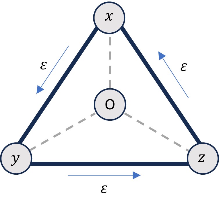
Consider the graph in Fig. 1.
Refer to caption
Figure 1: A merry-go-round graph with three states xyzx𝑥𝑦𝑧𝑥x\leftrightarrow y\leftrightarrow z\leftrightarrow x on a loop, and possible transitions to a sink/source state o𝑜o in the center.

The transition rates between the corner states and the central state are k(x,o)=k(y,o)=k(z,o)=eβ2μeβΔ𝑘𝑥𝑜𝑘𝑦𝑜𝑘𝑧𝑜superscript𝑒𝛽2𝜇superscript𝑒𝛽Δk(x,o)=k(y,o)=k(z,o)=e^{\frac{\beta}{2}\mu}e^{-\beta\Delta}, k(o,x)=k(o,y)=k(o,z)=eβ2μeβΔ𝑘𝑜𝑥𝑘𝑜𝑦𝑘𝑜𝑧superscript𝑒𝛽2𝜇superscript𝑒𝛽Δk(o,x)=k(o,y)=k(o,z)=e^{-\frac{\beta}{2}\mu}e^{-\beta\Delta} and the rates on the merry-go-round are

k(x,y)=k(y,z)=k(z,x)=11+eβε,k(x,z)=k(z,y)=k(y,x)=11+eβε.formulae-sequence𝑘𝑥𝑦𝑘𝑦𝑧𝑘𝑧𝑥11superscript𝑒𝛽𝜀𝑘𝑥𝑧𝑘𝑧𝑦𝑘𝑦𝑥11superscript𝑒𝛽𝜀k(x,y)=k(y,z)=k(z,x)=\frac{1}{1+e^{-\beta\varepsilon}},\quad k(x,z)=k(z,y)=k(y,x)=\frac{1}{1+e^{\beta\varepsilon}}.

The driving is ε𝜀\varepsilon giving a clockwise bias.
From (II.1)italic-(II.1italic-)\eqref{ldb}, the heat are

q(x,o)=q(y,o)=q(z,o)=μ,q(x,y)=q(y,z)=q(z,x)=εformulae-sequence𝑞𝑥𝑜𝑞𝑦𝑜𝑞𝑧𝑜𝜇𝑞𝑥𝑦𝑞𝑦𝑧𝑞𝑧𝑥𝜀q(x,o)=q(y,o)=q(z,o)=\mu,\qquad q(x,y)=q(y,z)=q(z,x)=\varepsilon

For fixed β𝛽\beta, to second order in ε𝜀\varepsilon, the quasipotentials are

V(x)=V(y)=V(z)=(μ3μeβμ+3)+βe12β(Δ+3μ)2(eβμ+3)2ε2+O(ε3)𝑉𝑥𝑉𝑦𝑉𝑧𝜇3𝜇superscript𝑒𝛽𝜇3𝛽superscript𝑒12𝛽Δ3𝜇2superscriptsuperscript𝑒𝛽𝜇32superscript𝜀2𝑂superscript𝜀3\displaystyle V(x)=V(y)=V(z)=\left(\mu-\frac{3\,\mu}{e^{\beta\,\mu\,}+3}\right)+\frac{\beta\,e^{\frac{1}{2}\beta\,(\Delta+3\,\mu)}}{2\left(e^{\beta\,\mu}+3\right)^{2}}\,\varepsilon^{2}+O\left(\varepsilon\,^{3}\right) (VI.1)
V(o)=3μeβμ+33βe12β(Δ+μ)2(eβμ+3)2ε2+O(ε3)𝑉𝑜3𝜇superscript𝑒𝛽𝜇33𝛽superscript𝑒12𝛽Δ𝜇2superscriptsuperscript𝑒𝛽𝜇32superscript𝜀2𝑂superscript𝜀3\displaystyle V(o)=-\frac{3\,\mu}{e^{\beta\,\mu}+3}-\frac{3\,\,\beta\,e^{\frac{1}{2}\beta(\Delta+\mu)}}{2\left(e^{\beta\mu}+3\right)^{2}}\,\varepsilon^{2}+O\left(\varepsilon^{3}\right) (VI.2)

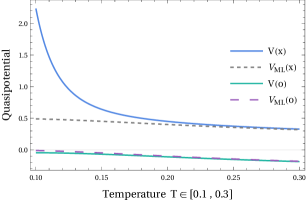
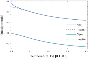
The second order term can diverge for β𝛽absent\beta\uparrow. Indeed, the quasipotential is not bounded for β𝛽absent\beta\uparrow when ΔΔ\Delta is large with respect to |μ|𝜇|\mu|. Yet, the linear term remains bounded, and corresponds to the quasipotential VML=EEML+Wsubscript𝑉𝑀𝐿𝐸subscriptdelimited-⟨⟩𝐸ML𝑊V_{ML}=E-\langle E\rangle_{\text{ML}}+W in the McLennan regime. See Fig. 2, where the quasipotentials given in (II.4) are plotted for ε=0.01𝜀0.01\varepsilon=0.01 and ε=0.05𝜀0.05\varepsilon=0.05. The dashed lines are for the McLennan quasipotentials VMLsubscript𝑉MLV_{\text{ML}}. If ε=0.05𝜀0.05\varepsilon=0.05, then the quasipotential of state o𝑜o is diverging at low temperature and is not bounded. For ε=0.01𝜀0.01\varepsilon=0.01 the quasipotentials of all states are bounded, and the extended Third law is broken only from second order around equilibrium.
Refer to caption
Refer to caption
Figure 2: Quasipotentials of Fig. 1. Δ=1.5,μ=0.5formulae-sequenceΔ1.5𝜇0.5\Delta=1.5,\,\mu=0.5, left: ε=0.05𝜀0.05\varepsilon=0.05 and right: ε=0.01𝜀0.01\varepsilon=0.01.

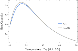
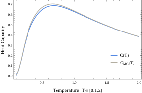
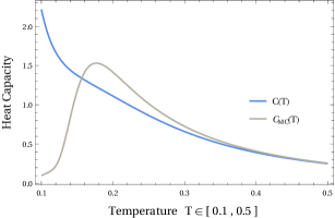
See Fig. 3, where the heat capacities in two different regimes are plotted. We plot the heat capacity given in (IV.1) where the average is over the general stationary distributions and V𝑉V is obtained from (II.4), this heat capacity is denoted by C(T)𝐶𝑇C(T). The heat capacity in the McLennan regime is denoted by CML(T)subscript𝐶ML𝑇C_{\text{ML}}(T) and is calculated from (IV.3).
C(T)𝐶𝑇C(T) and CML(T)subscript𝐶ML𝑇C_{\text{ML}}(T) are plotted for two different values of ε𝜀\varepsilon, left is for ε=0.05𝜀0.05\varepsilon=0.05 and the right figure is for ε=0.01𝜀0.01\varepsilon=0.01. The smaller driving leads the lines to overlap properly, and we did not put them here.
Refer to caption
Refer to caption
Figure 3: Heat capacity of Fig. 1. Δ=1.5,μ=0.5formulae-sequenceΔ1.5𝜇0.5\Delta=1.5,\,\mu=0.5, left: ε=0.05𝜀0.05\varepsilon=0.05 and right: ε=0.01𝜀0.01\varepsilon=0.01.

We see in fact that the McLennan expression of the heat capacity is a very good approximation to very low temperatures (but not to absolute zero).

Example VI.2 (Loop-tree).

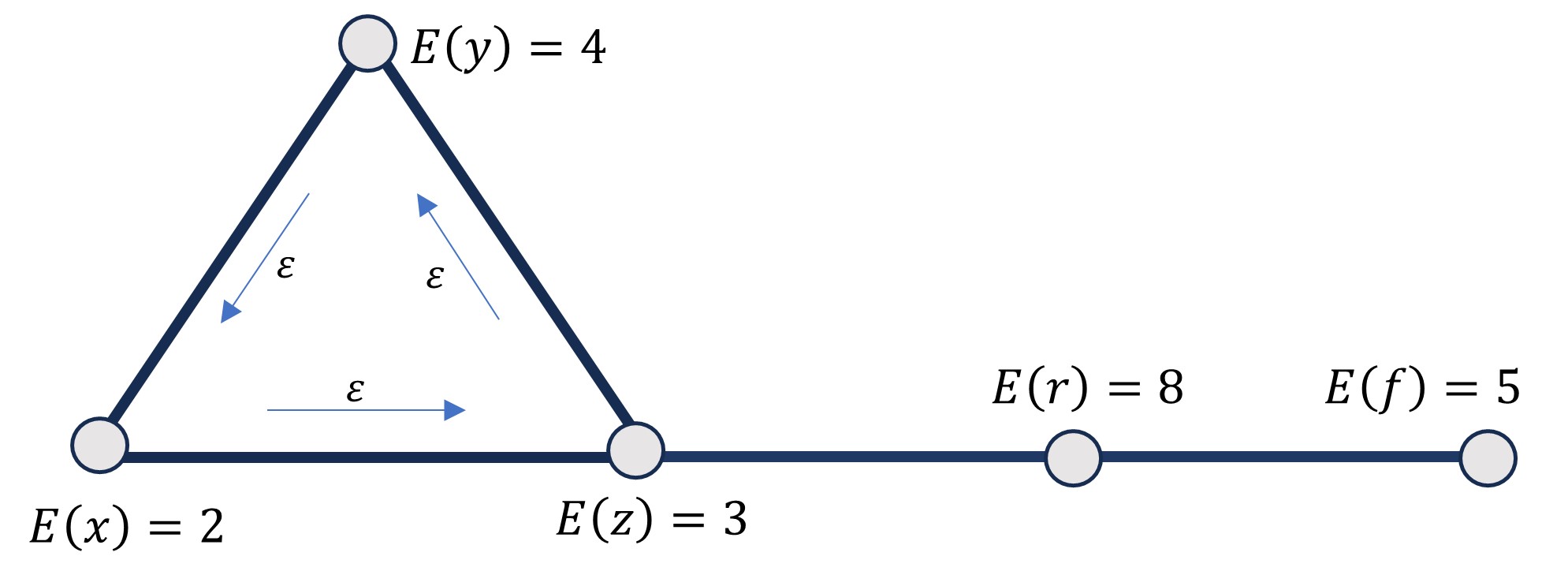
Consider a random walker jumping on the graph in Fig. 4. The transition rates for the jumps uu𝑢superscript𝑢u\rightarrow u^{\prime} are

k(u,u)=11+eβ(E(u)E(u)+s(u,u)),s(u,u)=s(u,u)formulae-sequence𝑘𝑢superscript𝑢11superscript𝑒𝛽𝐸𝑢𝐸superscript𝑢𝑠𝑢superscript𝑢𝑠𝑢superscript𝑢𝑠superscript𝑢𝑢k(u,u^{\prime})=\frac{1}{1+e^{-\beta(E(u)-E(u^{\prime})+s(u,u^{\prime}))}},\qquad s(u,u^{\prime})=-s(u^{\prime},u)

where s(x,z)=s(z,y)=s(y,x)=ε𝑠𝑥𝑧𝑠𝑧𝑦𝑠𝑦𝑥𝜀s(x,z)=s(z,y)=s(y,x)=\varepsilon, s(z,r)=s(r,f)=0𝑠𝑧𝑟𝑠𝑟𝑓0s(z,r)=s(r,f)=0, and the energy E𝐸E of each state is given in Fig. 4.

Refer to caption
Figure 4: A loop with a connected tree.

The heat are obtained from (II.1),

q(x,z)=1+ε,q(z,y)=1+ε,q(y,x)=2+ε,q(z,r)=5,q(r,f)=3formulae-sequence𝑞𝑥𝑧1𝜀formulae-sequence𝑞𝑧𝑦1𝜀formulae-sequence𝑞𝑦𝑥2𝜀formulae-sequence𝑞𝑧𝑟5𝑞𝑟𝑓3q(x,z)=-1+\varepsilon,\,\,q(z,y)=-1+\varepsilon,\,\,q(y,x)=2+\varepsilon,\,\,q(z,r)=-5,\,\,q(r,f)=3

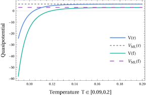
In Fig.5, we plot the quasipotentials V𝑉V defined in (II.4), together with their McLennan approximations VML=EEML+Wsubscript𝑉𝑀𝐿𝐸subscriptdelimited-⟨⟩𝐸ML𝑊V_{ML}=E-\langle E\rangle_{\text{ML}}+W. The (zero-temperature) boundedness of V(x)𝑉𝑥V(x), V(y)𝑉𝑦V(y) and V(z)𝑉𝑧V(z) depends on ε𝜀\varepsilon: for small ε𝜀\varepsilon they are bounded, but they are not bounded for ε=0.7𝜀0.7\varepsilon=0.7. V(r)𝑉𝑟V(r) and V(f)𝑉𝑓V(f) are diverging for any nonzero ε𝜀\varepsilon. However, the McLennan approximations VMLsubscript𝑉𝑀𝐿V_{ML} are uniformly bounded for all states.

Refer to caption
Refer to caption
Figure 5: Quasipotentials V𝑉V and VMLsubscript𝑉MLV_{\text{ML}} for the dynamics on Fig. 4. Left: quasipotentials of x,y𝑥𝑦x,y and z𝑧z for ε=0.7𝜀0.7\varepsilon=0.7, right: quasipotentials of states r𝑟r and f𝑓f when ε=0.003𝜀0.003\varepsilon=0.003.

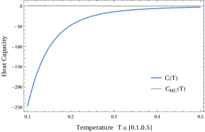
The McLennan heat capacity (IV.2) and the (full) heat capacity (IV.1) are plotted in Fig. 6. The plots are for two different ε𝜀\varepsilon. For small ε𝜀\varepsilon, CML(T)subscript𝐶ML𝑇C_{\text{ML}}(T) tends to overlap with C(T)𝐶𝑇C(T), even at low temperatures. That is no longer true for larger ε𝜀\varepsilon.

Refer to caption
Refer to caption
Figure 6: Heat capacity of Fig. 4. Left: ε=0.65𝜀0.65\varepsilon=0.65, right: ε=0.1𝜀0.1\varepsilon=0.1.

VII Conclusions

The thermal response around equilibrium is closely related to the static fluctuations in the McLennan ensemble. The quasipotential is connecting both features, as it is a measure of excess heat on the one hand, and on the other hand yielding the occupation statistics. It is therefore an extension of the useful relation between fluctuations and dissipation as we know it in equilibrium.
The resulting McLennan heat capacity (which is the heat capacity close to equilibrium) can be given entirely in terms of energy expectations (extending the even simpler formula for canonical equilibrium), and is derivable from an entropy. As the linear part around equilibrium of the nonequilibrium heat capacity, that McLennan heat capacity is always nonnegative and tends to zero with vanishing temperature. The breaking of the extended Third Law is therefore a nonlinear effect, starting only at second order.
We have added simple examples to illustrate these key-points.

Appendix A Graphical solution of Poisson equation

Lemma A.1.

W𝑊W in V is satisfying the equation:

LeqW(x)=ykeq(x,y)w(x,y)subscript𝐿eq𝑊𝑥subscript𝑦subscript𝑘eq𝑥𝑦𝑤𝑥𝑦L_{\text{eq}}W(x)=-\sum_{y}k_{\text{eq}}(x,y)w(x,y)
Proof.
LeqW(x)subscript𝐿eq𝑊𝑥\displaystyle L_{\text{eq}}W(x) =ykeq(x,y)(W(y)W(x))absentsubscript𝑦subscript𝑘eq𝑥𝑦𝑊𝑦𝑊𝑥\displaystyle=\sum_{y}k_{\text{eq}}(x,y)(W(y)-W(x))
=1meqykeq(x,y)z𝒱τz𝒯zmeq(τz)(ωτ(yz)ωτ(xz))absent1subscript𝑚eqsubscript𝑦subscript𝑘eq𝑥𝑦subscript𝑧𝒱subscriptsubscript𝜏𝑧subscript𝒯𝑧subscript𝑚eqsubscript𝜏𝑧subscript𝜔𝜏𝑦𝑧subscript𝜔𝜏𝑥𝑧\displaystyle=\frac{1}{m_{\text{eq}}}\sum_{y}k_{\text{eq}}(x,y)\,\sum_{z\in\mathcal{V}}\,\sum_{\tau_{z}\in\mathcal{T}_{z}}\,\,m_{\text{eq}}(\tau_{z})\big{(}\omega_{\tau}(y\to z)-\omega_{\tau}(x\to z)\big{)}
=1mykeq(x,y)z𝒱τz𝒯zmeq(τz)ωτ(yx)absent1𝑚subscript𝑦subscript𝑘eq𝑥𝑦subscript𝑧𝒱subscriptsubscript𝜏𝑧subscript𝒯𝑧subscript𝑚eqsubscript𝜏𝑧subscript𝜔𝜏𝑦𝑥\displaystyle=\frac{1}{m}\sum_{y}k_{\text{eq}}(x,y)\,\sum_{z\in\mathcal{V}}\,\sum_{\tau_{z}\in\mathcal{T}_{z}}\,\,m_{\text{eq}}(\tau_{z})\omega_{\tau}(y\to x)
=1meqykeq(x,y)z𝒱(τz(y,x)meq(τz)ωτ(yx)+τz∌(y,x)meq(τz)ωτ(yx))absent1subscript𝑚eqsubscript𝑦subscript𝑘eq𝑥𝑦subscript𝑧𝒱subscript𝑦𝑥subscript𝜏𝑧subscript𝑚eqsubscript𝜏𝑧subscript𝜔𝜏𝑦𝑥subscript𝑦𝑥subscript𝜏𝑧subscript𝑚eqsubscript𝜏𝑧subscript𝜔𝜏𝑦𝑥\displaystyle=\frac{1}{m_{\text{eq}}}\sum_{y}k_{\text{eq}}(x,y)\,\sum_{z\in\mathcal{V}}\big{(}\,\sum_{\tau_{z}\ni(y,x)}\,\,m_{\text{eq}}(\tau_{z})\omega_{\tau}(y\to x)+\sum_{\tau_{z}\not\ni(y,x)}\,\,m_{\text{eq}}(\tau_{z})\omega_{\tau}(y\to x)\big{)}

where in the third line the antisymmetric of w(u,u)𝑤𝑢superscript𝑢w(u,u^{\prime}) is used. If the tree τ𝜏\tau includes the edge (y,x)𝑦𝑥(y,x), then the path between y𝑦y to x𝑥x within the tree τ𝜏\tau is exactly the edge (y,x)𝑦𝑥(y,x), implying ωτ(yx)=w(y,x)subscript𝜔𝜏𝑦𝑥𝑤𝑦𝑥\omega_{\tau}(y\to x)=w(y,x) and hence,

LeqW(x)subscript𝐿eq𝑊𝑥\displaystyle L_{\text{eq}}W(x) =1meqykeq(x,y)z𝒱(τz(y,x)meq(τz)w(y,x)+τz∌(y,x)meq(τz)ωτ(yx))absent1subscript𝑚eqsubscript𝑦subscript𝑘eq𝑥𝑦subscript𝑧𝒱subscript𝑦𝑥subscript𝜏𝑧subscript𝑚eqsubscript𝜏𝑧𝑤𝑦𝑥subscript𝑦𝑥subscript𝜏𝑧subscript𝑚eqsubscript𝜏𝑧subscript𝜔𝜏𝑦𝑥\displaystyle=\frac{1}{m_{\text{eq}}}\sum_{y}k_{\text{eq}}(x,y)\,\sum_{z\in\mathcal{V}}\big{(}\,\sum_{\tau_{z}\ni(y,x)}\,\,m_{\text{eq}}(\tau_{z})w(y,x)+\sum_{\tau_{z}\not\ni(y,x)}\,\,m_{\text{eq}}(\tau_{z})\omega_{\tau}(y\to x)\big{)}
=ykeq(x,y)w(y,x)1meqz𝒱(τz(y,x)meq(τz)+τz∌(y,x)meq(τz))absentsubscript𝑦subscript𝑘eq𝑥𝑦𝑤𝑦𝑥1subscript𝑚eqsubscript𝑧𝒱subscript𝑦𝑥subscript𝜏𝑧subscript𝑚eqsubscript𝜏𝑧subscript𝑦𝑥subscript𝜏𝑧subscript𝑚eqsubscript𝜏𝑧\displaystyle=\sum_{y}k_{\text{eq}}(x,y)w(y,x)\,\frac{1}{m_{\text{eq}}}\sum_{z\in\mathcal{V}}\big{(}\,\sum_{\tau_{z}\ni(y,x)}\,\,m_{\text{eq}}(\tau_{z})+\sum_{\tau_{z}\not\ni(y,x)}\,\,m_{\text{eq}}(\tau_{z})\big{)} (A.1)
+1meqykeq(x,y)z𝒱(τz∌(y,x)meq(τz)w(y,x)+τz∌(y,x)meq(τz)ωτ(yx))1subscript𝑚eqsubscript𝑦subscript𝑘eq𝑥𝑦subscript𝑧𝒱subscript𝑦𝑥subscript𝜏𝑧subscript𝑚eqsubscript𝜏𝑧𝑤𝑦𝑥subscript𝑦𝑥subscript𝜏𝑧subscript𝑚eqsubscript𝜏𝑧subscript𝜔𝜏𝑦𝑥\displaystyle\quad+\frac{1}{m_{\text{eq}}}\sum_{y}k_{\text{eq}}(x,y)\sum_{z\in\mathcal{V}}\big{(}-\sum_{\tau_{z}\not\ni(y,x)}\,\,m_{\text{eq}}(\tau_{z})w(y,x)+\sum_{\tau_{z}\not\ni(y,x)}\,\,m_{\text{eq}}(\tau_{z})\omega_{\tau}(y\to x)\big{)}
=ykeq(x,y)w(x,y)+1meqy,zkeq(x,y)τz∌(y,x)meq(τz)(w(x,y)+ωτ(yx))absentsubscript𝑦subscript𝑘eq𝑥𝑦𝑤𝑥𝑦1subscript𝑚eqsubscript𝑦𝑧subscript𝑘eq𝑥𝑦subscript𝑦𝑥subscript𝜏𝑧subscript𝑚eqsubscript𝜏𝑧𝑤𝑥𝑦subscript𝜔𝜏𝑦𝑥\displaystyle=-\sum_{y}k_{\text{eq}}(x,y)w(x,y)+\frac{1}{m_{\text{eq}}}\sum_{y,z}k_{\text{eq}}(x,y)\sum_{\tau_{z}\not\ni(y,x)}\,\,m_{\text{eq}}(\tau_{z})\big{(}w(x,y)+\omega_{\tau}(y\to x)\big{)}

We show that the second sum in the last line equals zero.

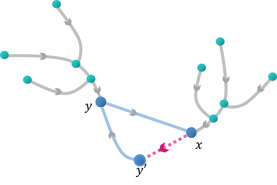
If z=x𝑧𝑥z=x, fix a spanning tree τ𝜏\tau such that (x,y)τx𝑥𝑦subscript𝜏𝑥(x,y)\not\in\tau_{x}. There is a path between x𝑥x and y𝑦y in the tree, and adding the edge (x,y)𝑥𝑦(x,y) to τxsubscript𝜏𝑥\tau_{x} creates a loop with some rooted tree connected to the loop. That loop is made by the path τ(yx)𝜏𝑦𝑥\tau(y\to x) together with the edge (x,y)𝑥𝑦(x,y). The vertex x𝑥x has another neighbor in that loop that we call ysuperscript𝑦y^{\prime}. There exists a spanning tree made by removing the edge (y,x)superscript𝑦𝑥(y^{\prime},x) from the tree τ𝜏\tau and adding the edge (y,x)𝑦𝑥(y,x); we call it τsuperscript𝜏\tau^{\prime}. Now adding the edge (x,y)𝑥superscript𝑦(x,y^{\prime}) to the spanning tree τzsubscriptsuperscript𝜏𝑧\tau^{\prime}_{z} makes a loop with some rooted tree connected to the loop. That loop is made by the path τ(yx)superscript𝜏superscript𝑦𝑥\tau^{\prime}(y^{\prime}\to x) together with (x,y)𝑥superscript𝑦(x,y^{\prime}). As a result, the graphs τx(x,y)subscript𝜏𝑥𝑥𝑦\tau_{x}\cup(x,y) and τx(x,y)subscriptsuperscript𝜏𝑥𝑥superscript𝑦\tau^{\prime}_{x}\cup(x,y^{\prime}) have different directions in the loop but the rest is similar; see Fig. 7.
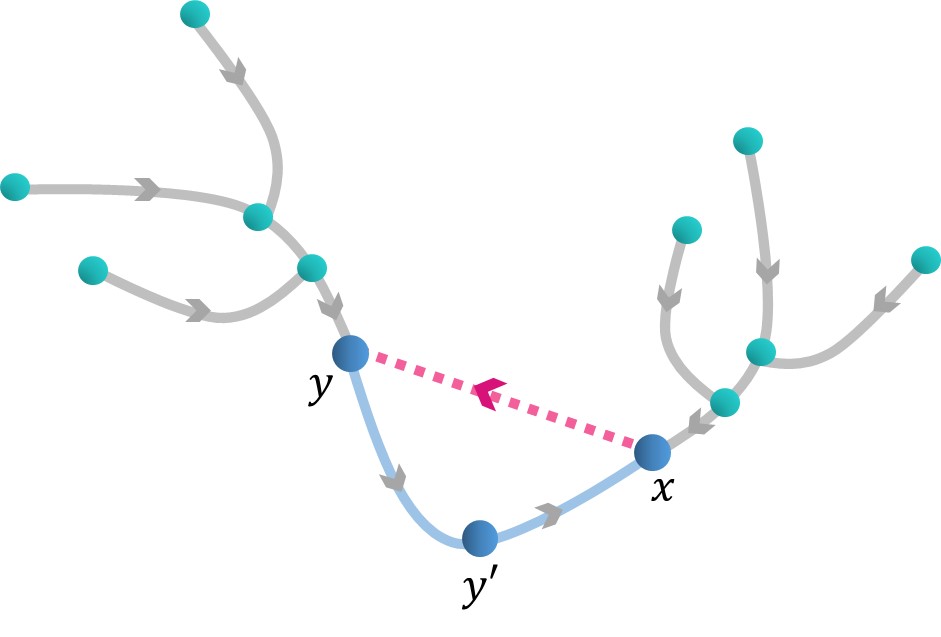
Refer to caption
(a) τx(x,y)subscript𝜏𝑥𝑥𝑦\tau_{x}\cup(x,y)
Refer to caption
(b) τx(x,y)subscriptsuperscript𝜏𝑥𝑥superscript𝑦\tau^{\prime}_{x}\cup(x,y^{\prime})
Figure 7: Adding (x,y)𝑥𝑦(x,y) to τxsubscript𝜏𝑥\tau_{x} and the edge (x,y)𝑥superscript𝑦(x,y^{\prime}) to t τxsubscriptsuperscript𝜏𝑥\tau^{\prime}_{x} makes two graphs which are different only in the direction of their unique loop.

From detailed balanced, two different directions of a loop have the same weight and

meq(τx)keq(x,y)=meq(τx)k(x,y)subscript𝑚eqsubscript𝜏𝑥subscript𝑘eq𝑥𝑦subscript𝑚eqsubscriptsuperscript𝜏𝑥𝑘𝑥superscript𝑦m_{\text{eq}}(\tau_{x})\,k_{\text{eq}}(x,y)=m_{\text{eq}}(\tau^{\prime}_{x})\,k(x,y^{\prime})

Therefore, by the antisymmetry of w(x,y)𝑤𝑥𝑦w(x,y),

meq(τx)keq(x,y)(w(y,x)+ωτ(xy))+meq(τx)keq(x,y)(w(y,x)+ωτ(xy))=0subscript𝑚eqsubscript𝜏𝑥subscript𝑘eq𝑥𝑦𝑤𝑦𝑥subscript𝜔𝜏𝑥𝑦subscript𝑚eqsubscriptsuperscript𝜏𝑥subscript𝑘eq𝑥superscript𝑦𝑤superscript𝑦𝑥superscriptsubscript𝜔𝜏𝑥superscript𝑦0\displaystyle m_{\text{eq}}(\tau_{x})\,k_{\text{eq}}(x,y)(w(y,x)+\omega_{\tau}(x\to y))+m_{\text{eq}}(\tau^{\prime}_{x})\,k_{\text{eq}}(x,y^{\prime})(w(y^{\prime},x)+\omega_{\tau}^{\prime}(x\to y^{\prime}))=0

where w(y,x)+ωτ(xy)𝑤𝑦𝑥subscript𝜔𝜏𝑥𝑦w(y,x)+\omega_{\tau}(x\to y) and w(y,x)+ωτ(xy)𝑤superscript𝑦𝑥subscript𝜔𝜏𝑥superscript𝑦w(y^{\prime},x)+\omega_{\tau}(x\to y^{\prime}) are sums over the w(u,u)𝑤𝑢superscript𝑢w(u,u^{\prime}) of the edges of the same loop but in two different directions. Hence,

1meqykeq(x,y)τx∌(y,x)meq(τx)(w(x,y)+ωτ(yx)=0\frac{1}{m_{\text{eq}}}\sum_{y}k_{\text{eq}}(x,y)\sum_{\tau_{x}\not\ni(y,x)}\,\,m_{\text{eq}}(\tau_{x})\big{(}w(x,y)+\omega_{\tau}(y\to x)=0 (A.2)

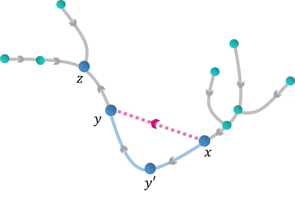
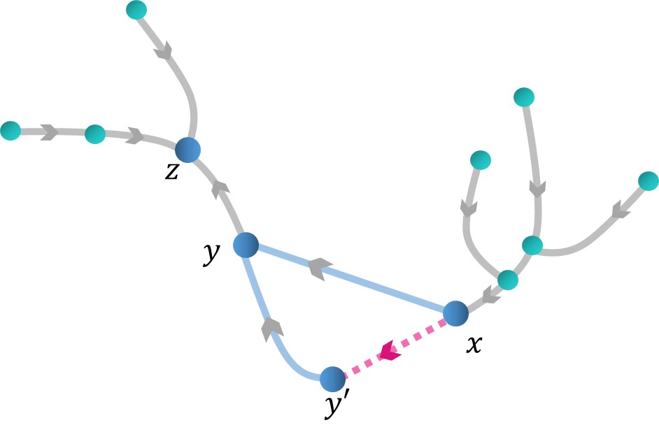
If zx𝑧𝑥z\not=x, take a spanning tree τ𝜏\tau such that (x,y)τ𝑥𝑦𝜏(x,y)\not\in\tau. There is a path between x𝑥x and y𝑦y in the tree. Adding the edge (x,y)𝑥𝑦(x,y) to τzsubscript𝜏𝑧\tau_{z} makes a loop with some rooted tree connected to the loop. That loop is made by the path τ(yx)𝜏𝑦𝑥\tau(y\to x) together with the edge (x,y)𝑥𝑦(x,y), but the edges on that loop are not oriented in one direction. The vertex x𝑥x has another neighbour in this loop that we call ysuperscript𝑦y^{\prime}. There exists a spanning tree made by removing the edge (y,x)superscript𝑦𝑥(y^{\prime},x) from the tree τ𝜏\tau and adding the edge (y,x)𝑦𝑥(y,x); we call it τsuperscript𝜏\tau^{\prime}. Now adding the edge (x,y)𝑥superscript𝑦(x,y^{\prime}) to the spanning tree τzsubscriptsuperscript𝜏𝑧\tau^{\prime}_{z} makes a loop with some rooted tree connected to the loop. This loop is made by the path τ(yx)superscript𝜏superscript𝑦𝑥\tau^{\prime}(y^{\prime}\to x) together with (x,y)𝑥superscript𝑦(x,y^{\prime}). The graphs τx(x,y)subscript𝜏𝑥𝑥𝑦\tau_{x}\cup(x,y) and τx(x,y)subscriptsuperscript𝜏𝑥𝑥superscript𝑦\tau^{\prime}_{x}\cup(x,y^{\prime}) are the same; see Fig. 8.

Refer to caption
(a) τz(x,y)subscript𝜏𝑧𝑥𝑦\tau_{z}\cup(x,y)
Refer to caption
(b) τz(x,y)subscriptsuperscript𝜏𝑧𝑥superscript𝑦\tau^{\prime}_{z}\cup(x,y^{\prime})
Figure 8: Adding (x,y)𝑥𝑦(x,y) to τzsubscript𝜏𝑧\tau_{z} and the edge (x,y)𝑥superscript𝑦(x,y^{\prime}) to τzsubscriptsuperscript𝜏𝑧\tau^{\prime}_{z} makes two same graphs

Hence,

meq(τz)keq(x,y)(w(y,x)+ωτ(xy))+meq(τz)keq(x,y)(w(y,x)+ωτ(xy))=0subscript𝑚eqsubscript𝜏𝑧subscript𝑘eq𝑥𝑦𝑤𝑦𝑥subscript𝜔𝜏𝑥𝑦subscript𝑚eqsubscriptsuperscript𝜏𝑧subscript𝑘eq𝑥superscript𝑦𝑤superscript𝑦𝑥superscriptsubscript𝜔𝜏𝑥superscript𝑦0\displaystyle m_{\text{eq}}(\tau_{z})\,k_{\text{eq}}(x,y)(w(y,x)+\omega_{\tau}(x\to y))+m_{\text{eq}}(\tau^{\prime}_{z})\,k_{\text{eq}}(x,y^{\prime})(w(y^{\prime},x)+\omega_{\tau}^{\prime}(x\to y^{\prime}))=0

where w(y,x)+ωτ(xy)𝑤𝑦𝑥subscript𝜔𝜏𝑥𝑦w(y,x)+\omega_{\tau}(x\to y) and w(y,x)+ωτ(xy)𝑤superscript𝑦𝑥subscript𝜔𝜏𝑥superscript𝑦w(y^{\prime},x)+\omega_{\tau}(x\to y^{\prime}) are sums over all w(u,u)𝑤𝑢superscript𝑢w(u,u^{\prime}) over the edges of the same loop in two different directions. We conclude that

1meqy,zkeq(x,y)τz∌(y,x)meq(τz)(w(x,y)+ωτ(yx)=0\frac{1}{m_{\text{eq}}}\sum_{y,z}k_{\text{eq}}(x,y)\sum_{\tau_{z}\not\ni(y,x)}\,\,m_{\text{eq}}(\tau_{z})\big{(}w(x,y)+\omega_{\tau}(y\to x)=0 (A.3)

and the proof is finished. ∎

References

  • [1] P. Dolai, C. Maes, and K. Netočný. Calorimetry for active systems. SciPost Phys., 14:126, (2023).
  • [2] F. Khodabandehlou, S. Krekels, and I. Maes. Exact computation of heat capacities for active particles on a graph. J. Stat. Mech.: Theory and Experiment, 2022(12):123208, (2022).
  • [3] P. Dolai and C. Maes. Specific heat of a driven fermionic array. SSRN, https://ssrn.com/abstract=4509172, (2023).
  • [4] F. Khodabandehlou, C. Maes, and K. Netočný. A Nernst heat theorem for nonequilibrium jump processes. J. Chem. Phys., 158(20), (2023).
  • [5] F. Khodabandehlou and I. Maes. Drazin-Inverse and heat capacity for driven random walks on the ring. arXiv, 2204.04974 [math.PR], (2023).
  • [6] Y. Oono and M. Paniconi. Steady State Thermodynamics. Progr. Theor. Phys. Suppl., 130:29–44, (1998).
  • [7] T. S. Komatsu, N. Nakagawa, S. I. Sasa, and H. Tasaki. Steady-state thermodynamics for heat conduction: Microscopic derivation. Phys. Rev. Lett., 100(23), (2008).
  • [8] T. S. Komatsu, N. Nakagawa, S. Sasa, and H. Tasaki. Representation of nonequilibrium steady states in large mechanical systems. J. Stat. Phys, 134(2):401–423, (2009).
  • [9] F. Khodabandehlou, C. Maes, I. Maes, and K. Netočný. The vanishing of excess heat for nonequilibrium processes reaching zero ambient temperature. arXiv, 2210.09858 [cond-mat.stat-mech], (2023).
  • [10] E. Boksenbojm, C. Maes, K. Netočný, and J. Pešek. Heat capacity in nonequilibrium steady states. Europhys. Lett., 96(4):40001, (2011).
  • [11] J. Pešek, E. Boksenbojm, and K. Netočný. Model study on steady heat capacity in driven stochastic systems. Open Physics, 10(3), (2012).
  • [12] U. Basu, C. Maes, and K. Netočný. Statistical forces from close-to-equilibrium media. New J. Phys., 17(11):115006, (2015).
  • [13] J. A. McLennan. Statistical mechanics of the steady state. Phys. Rev., 115:1405–1409, (1959).
  • [14] C. Maes and K. Netočný. Rigorous meaning of McLennan ensembles. J. Math. Phys., 51(1), (2010).
  • [15] I. Prigogine and P. Résibois. On the kinetics of the approach to equilibrium. Physica, 27(7):629–646, (1961).
  • [16] S. Nakajima. On quantum theory of transport phenomena: Steady diffusion. Prog. Theor. Phys., 20(6):948–959, (1958).
  • [17] R. Zwanzig. Ensemble method in the theory of irreversibility. J. Chem. Phys., 33(5):1338, (1960).
  • [18] R. Zwanzig. Ensemble method in the theory of irreversibility. Lect. Theor. Phys, 33(5):106–141, (1960).
  • [19] C. Maes. Local detailed balance. SciPost Phys. Lect. Notes, page 32, (2021).
  • [20] G. Grimmett and D. Stirzaker. Probability and random processes. Oxford University Press, Oxford; New York, 2001.
  • [21] C. Kipnis, C. Marchioro, and E. Presutti. Heat flow in an exactly solvable model,. J.  Stat.  Phys. , 27(1):65–74, (1982).
  • [22] C. Franceschini, R. Frassek, and C. Giardinà . Integrable heat conduction model. J. Math. Phys. , 64(4):043304, apr (2023).
  • [23] G. Carinci, C. Franceschini, D. Gabrielli, C. Giardinà, and D. Tsagkarogiannis. Solvable stationary non equilibrium states. arXiv, 2307.02793 [math.PR], (2023).
  • [24] C. Maes and K. Netočný. Nonequilibrium calorimetry. J. Stat. Mech.: Theory and Experiment, 2019(11):114004, (2019).
  • [25] L. Bertini, D. Gabrielli, G. Jona-Lasinio, and C. Landim. Thermodynamic transformations of nonequilibrium states. J. Stat. Phys, 149(5):773–802, (2012).
  • [26] L. Bertini, D. Gabrielli, G. Jona-Lasinio, and C. Landim. Clausius inequality and optimality of quasistatic transformations for nonequilibrium stationary states. Phys.  Rev.  Lett., 110(2), (2013).
  • [27] T. S. Komatsu and N. Nakagawa. Expression for the stationary distribution in nonequilibrium steady states. Phys. Rev. Lett., 100:030601, (2008).
  • [28] C. Maes and K. Netočný. A nonequilibrium extension of the clausius heat theorem. J. Stat. Phys, 154(1-2):188–203, (2013).
  • [29] M. Aizenman and E. H. Lieb. The third law of thermodynamics and the degeneracy of the ground state for lattice systems. J. Stat. Phys., 24:279–297, (1981).
  • [30] F. Khodabandehlou, C. Maes, and K. Netočný. Trees and forests for nonequilibrium purposes: An introduction to graphical representations. J. Stat. Phys, 189:41, (2022).