Limited efficacy of forward contact tracing in epidemics

Abstract

Infectious diseases that spread silently through asymptomatic or pre-symptomatic infections represent a challenge for policy makers. A traditional way of achieving isolation of silent infectors from the community is through forward contact tracing, aiming at identifying individuals that might have been infected by a known infected person. In this work we investigate how efficient this measure is in preventing a disease from becoming endemic. We introduce an SIS-based compartmental model where symptomatic individuals may self-isolate and trigger a contact tracing process aimed at quarantining asymptomatic infected individuals. Imperfect adherence and delays affect both measures. We derive the epidemic threshold analytically and find that contact tracing alone can only lead to a very limited increase of the threshold. We quantify the effect of imperfect adherence and the impact of incentivizing asymptomatic and symptomatic populations to adhere to isolation. Our analytical results are confirmed by simulations on complex networks and by the numerical analysis of a much more complex model incorporating more realistic in-host disease progression.

Introduction

Containing the propagation of infectious diseases that are able to spread silently through asymptomatic or pre-symptomatic infections is particularly challenging Fraser et al. (2004); Ferretti et al. (2020); Johansson et al. (2021); Li et al. (2020); Groendyke and Combs (2021). A traditional way of achieving isolation of silent infectors without applying restrictive policies to entire populations (such as lockdowns) is through the so-called contact tracing (CT) measure, considered in the past to cope with outbreaks of SARS Riley et al. (2003); Lipsitch et al. (2003), Foot and Mouth disease Ferguson et al. (2001), smallpox Foege et al. (1971); Riley and Ferguson (2006), tubercolosis Fox et al. (2013), HIV Rutherford and Woo (1988), Ebola Saurabh and Prateek (2017); Swanson et al. (2018), SARS-CoV-2 Shin et al. (2020). Being at higher risk of infection, the contacts of a known infected person are retrieved and recommended to quarantine. However this measure still constitutes a considerable social burden, as it may isolate also healthy individuals from the community and requires intense logistical efforts for tracing contacts - a particularly difficult task for airborne-diseases like COVID-19. As fatigue sets in and adherence to isolation mandates and to pharmaceutical interventions fades Silva and Martin (2020), it is not clear under what conditions it is convenient to simplify the policies and rely only on case-isolation and vaccination strategies or when, instead, implementing CT is crucial for epidemic control. This is the question we tackle in this work.

The success of contact tracing in the past has not been universal. While some outbreaks could be controlled Gibney (2020), others required more intense interventions to achieve epidemic control Blakely et al. (2020); Knapton (2020). The efficacy of the contact tracing measure has been studied in a number of works, with various approaches ranging from stochastic simulations (Mancastroppa et al. (2021); Kerr et al. (2021); Burdinski et al. (2022); Groendyke and Combs (2021); Hellewell et al. (2020); Hasegawa and Nemoto (2017); Horstmeyer et al. (2022)) to analytical investigations (Lee et al. (2022); Heidecke et al. (2022); House and Keeling (2010); Reyna-Lara et al. (2021); Bianconi et al. (2021); Kojaku et al. (2021); Burgio et al. (2021); Rizi et al. (2022)).

The utility of contact tracing has often been considered in opposition to or in combination with other containment strategies. Hasegawa et al. Hasegawa and Nemoto (2017) found that quarantine measures outperform the random and acquaintance preventive vaccination schemes for what concerns transmission reduction. The work of Horstmeyer et al. Horstmeyer et al. (2022) suggested instead that a combination of self-distancing and isolation is particularly effective to contain a disease. Through a delay differential equation model, Heidecke et al. Heidecke et al. (2022) found that the efficacy of the test-trace-isolate-quarantine is limited and requires to be combined with other enhanced hygienic measures to achieve disease control. They also warned upon the self-acceleration of disease spread that can be caused by limited capacities of tracing.

Some works focused specifically on the contact tracing measure, investigating the role played by different parameters on its efficacy for the containment of the spread of infectious pathogens. Kerr et al. Kerr et al. (2021) and Burdinski et al. Burdinski et al. (2022) found that the efficacy of contact tracing improves with incidence. In the specific context of the early COVID-19 pandemic in Seattle, an agent-based model calibrated to demographic, mobility and epidemiological data predicted that the contact tracing measure would allow the reopening of society in the absence of massive vaccination coverage while maintaining epidemic control, if performed strongly, i.e. with high testing and tracing rates, high quarantine compliance, short testing and tracing delays and moderate mask use Kerr et al. (2021). Similarly, Reyna-Lana et al. Reyna-Lara et al. (2021) concluded, by means of a markovian treatment of a SIR model for the simultaneous contagion processes of infection and contact tracing, that the combination of case-isolation and contact tracing is beneficial to the outbreak containment but requires high adoption of digital contact tracing apps to identify superspreaders. Optimal app coverage was also studied by Bianconi et al. Bianconi et al. (2021) through a message-passing model. High app adoption, in particular by high-degree nodes, appeared to be crucial. However, adoption of digital contact tracing apps seems unlikely to be achieved by high degree nodes. Crucially, this was found by Mancastroppa et al. Mancastroppa et al. (2021) to undermine the performance of digital contact tracing compared to manual one, as a consequence of a quenched sampling from the population in contrast with an annealed one. Through numerical simulations, Hellewell et al. Hellewell et al. (2020) and Burdinski et al. Burdinski et al. (2022) concluded that efficacy of the forward contact tracing measure is limited.

According to the simulation work of Kojaku et al. Kojaku et al. (2021) on synthetic and empirical contact networks, tracing the potential infector of a known case instead of its potential infectees (backward instead of forward contact tracing) was exceptionally efficient at detecting superspreading events, since it leverages two statistical biases. Homophily in adoption of digital contact tracing apps leads to improved performance of contact tracing when coverage is low Rizi et al. (2022); Burgio et al. (2021). Also the clustering of networks, appears to favor CT performance in many settings House and Keeling (2010); Burdinski et al. (2022); Kiss et al. (2005).

Despite intense recent activity, an analytical understanding of the impact of imperfect adherence and implementation delays on the efficacy of contact tracing is still missing. In this work we fill this gap, by considering an SIS-based compartmental model for the self-isolation of symptomatic individuals and the quarantine of their asymptomatic contacts. More specifically, we study the influence of three kinds of imperfect adherence to self-isolation and to quarantine – delay to isolation, imperfect compliance and anticipated exit from isolation – on the value of the epidemic threshold. Within a mean-field approach, we derive an analytical expression for the epidemic threshold, defined as the critical virus transmissibility that separates a healthy absorbing phase from an endemic phase. This allows to evaluate the performance of contact tracing and compare it to the efficacy of self-isolation alone as a function of the parameters describing behavioral and physiological features of the population. We further determine analytically the role of the contact tracing measure on the stationary fractions of infected individuals. Finally, we show that heterogeneities in contact patterns and more complex in-host disease progression do not qualitatively alter the findings of the mean-field approach.

I The Model and its mean-field solution

The model we consider is a variation of the SIS-based epidemic model with self-isolation, delay and fatigue developed in Ref. de Meijere et al. (2021). We shall hereafter refer to it as ”IDF” (isolation-delay-fatigue).

According to the IDF dynamics (see Fig. 1(a)), the contact of a susceptible ($S$) individual with an infectious one (state $U$, $I$, or $F$, see below) leads to the infection of the former with rate $\beta$. Newly infected individuals are assumed to be immediately infectious but not yet settled on whether to enter isolation or not (undecided, $U$). After a time interval distributed with Poissonian rate $\mu_{U}$ they decide (with probability $p_{Q}$) whether to fully interrupt contacts with the rest of the population by entering the isolated compartment $Q$ or (with probability $1-p_{Q}$) to disregard their infectious state and keep the same rate of interactions with the community, by transitioning to the $I$ compartment. The delay between infection and isolation (of mean duration $T_{U}=1/\mu_{U}$) models logistical delays as well as behavioral ones. In order to account for isolated individuals exiting isolation before being fully recovered, as a consequence of fatigue, a transition from $Q$ to another infectious compartment (fatigued, $F$) occurs at rate $\mu_{Q}$.

In the present work, infected individuals are assumed to either stay asymptomatic through the whole infectious period (with probability $q_{A}$) or to develop symptoms (with the complementary probability $1-q_{A}$). For this reason the original $U$ compartment is split here into three compartments. Individuals developing symptoms enter compartment $U_{S}$ upon infection. Being aware of their infected status, symptomatic individuals all go through the decision process (still with rate $\mu_{U}$) on whether to isolate (going to state $Q$, with probability $p_{Q}^{S}$) or not (going to state $I$, with complementary probability $1-p_{Q}^{S}$). Asymptomatic individuals can instead only initiate the decision process if they are infected by a symptomatic individual (who traces them). We therefore distinguish between the asymptomatic individuals who are infected by a symptomatic individual $U_{S}$ and are thereby traced ($U_{A}^{+}$) and those who are not ($U_{A}^{-}$). Imperfect tracing capacity is taken into account with only a fraction $p_{CT}$ of the contacts of symptomatic individuals being successfully traced.

Symptoms are assumed to appear immediately upon infection and thus to lead to immediate tracing of the contacts of $U_{S}$ individuals. Traced asymptomatic individuals ($U_{A}^{+}$) decide with rate $\mu_{U}$ whether to enter the quarantined $Q$ state or not (thus transitioning to the $I$ state). As symptoms likely play a major role in determining compliance to containment measures, we consider the probability $p_{Q}^{A}$ that a traced asymptomatic decides to self-isolate distinct from (and in particular smaller than or at most equal to) the analogous probability $p_{Q}^{S}$ for a symptomatic individual. Again, individuals in $Q$ may exit isolation before being fully recovered by transitioning through compartment $F$, as a consequence of fatigue. We assume the same transmissibility across all infectious compartments $U_{A}^{-}$, $U_{A}^{+}$, $U_{S}$, $I$ and $F$ and perfect isolation of individuals while residing in compartment $Q$. As the progression of the disease does not depend on the isolation status, spontaneous recovery transitions may occur from states $U_{A}^{-}$, $U_{A}^{+}$, $U_{S}$, $I$, $Q$ and $F$ to the susceptible state $S$, at the same recovery rate $\mu$.

For a complete summary of all the transitions and their respective rates see Appendix VII. The parameters of the model are summarized in Table1. Fig. 1(b) presents a complete description of the epidemic compartments and the transition rates at the homogeneous mean-field level, where each individual has $\langle k\rangle$ contacts.

Table 1: Model parameters

Parameters	Description
$\beta$	rate of infection
$q_{A}$	share of asymptomatic
$\mu$	rate of recovery
$\mu_{U}$	rate of decision
$\mu_{Q}$	rate of exit from isolation
$p_{CT}$	probability of being traced
$p_{Q}^{S}$	compliance probability if symptomatic
$p_{Q}^{A}$	compliance probability if asymptomatic
$\langle k\rangle$	mean node degree

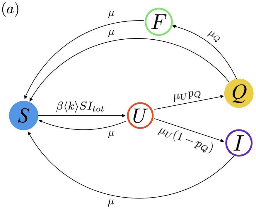
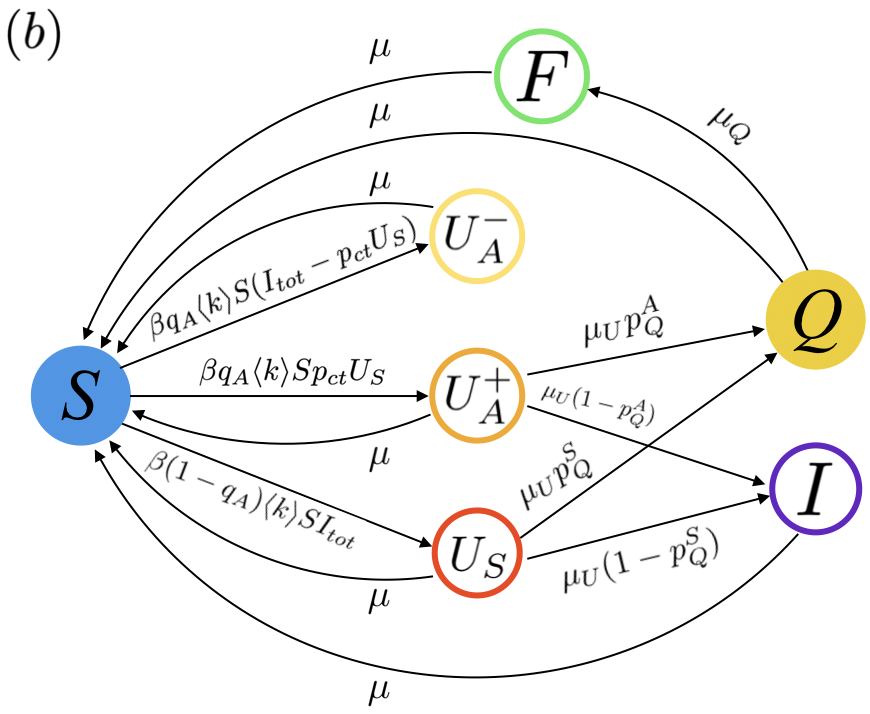
Figure 1: Schematic description of the transitions between compartments in (a) the model with self-isolation, delay, fatigue and (b) the same model with the addition of contact tracing. The quantity $I_{tot}$ is the fraction of individuals that are infectious: $I_{tot}=U+I+F$ in (a) and $I_{tot}=U_{S}+U_{A}^{+}+U_{A}^{-}+I+F$ in (b).

In this setting the dynamics of the fractions of individuals in states $U_{A}^{-}$, $U_{A}^{+}$, $U_{S}$, $Q$, $I$ and $F$ is governed by the following set of differential equations

$$\begin{cases}\dot{U}_{A}^{-}&=\beta q_{A}\langle k\rangle S(U_{A}^{-}+U_{A}^{+}+I+F+U_{S}(1-p_{CT}))+\\ &\hskip 260.17464pt-\mu U_{A}^{-}\\ \dot{U}_{A}^{+}&=\beta q_{A}\langle k\rangle SU_{S}p_{CT}-(\mu+\mu_{U})U_{A}^{+}\\ \dot{U}_{S}&=\beta(1-q_{A})\langle k\rangle S(U_{A}^{-}+U_{A}^{+}+I+F+U_{S})+\\ &\hskip 260.17464pt-(\mu+\mu_{U})U_{S}\\ \dot{Q}&=\mu_{U}p_{Q}^{A}U_{A}^{+}+\mu_{U}p_{Q}^{S}U_{S}-(\mu+\mu_{Q})Q\\ \dot{I}&=\mu_{U}(1-p_{Q}^{A})U_{A}^{+}+\mu_{U}(1-p_{Q}^{S})U_{S}-\mu I\\ \dot{F}&=\mu_{Q}Q-\mu F,\end{cases}$$ (1)

where the notation $\dot{X}=\frac{dX}{dt}$ indicates the time derivatives of the fractions of individuals in each compartment and $S=1-U_{A}^{-}-U_{A}^{+}-U_{S}-Q-I-F$.

The Jacobian matrix obtained by linearization around the disease-free equilibrium $(S,U_{A}^{-},U_{A}^{+},U_{S},I,Q,F)=(1,0,0,0,0,0,0)$ has 4 real eigenvalues that are always negative and 2 other real eigenvalues which become positive as $\lambda=\beta/\mu$ is increased. The largest one becomes positive (thus making the disease-free equilibrium unstable) above the epidemic threshold

$$\lambda_{c}=\frac{1-\sqrt{1-2\chi}}{\chi}\cdot\lambda_{c}^{IDF}(q_{A}),$$ (2)

where

$$\begin{cases}&\lambda_{c}^{IDF}(q_{A})=\frac{1}{\langle k\rangle}\frac{1}{1-\frac{p_{Q}^{S}(1-q_{A})}{(1+\frac{T_{U}}{T})(1+\frac{T}{T_{Q}})}}\\ &T=1/\mu\\ &T_{U}=1/\mu_{U}\\ &T_{Q}=1/\mu_{Q}\\ &\chi(q_{A},p_{Q}^{S},p_{Q}^{A})=\frac{2q_{A}(1-q_{A})(p_{CT}p_{Q}^{A})}{(1+\frac{T}{T_{U}})(1+\frac{T_{U}}{T})(1+\frac{T}{T_{Q}})}\times\\ &\hskip 130.08731pt\times\frac{1}{\left(1-\frac{p_{Q}^{S}(1-q_{A})}{(1+\frac{T_{U}}{T})(1+\frac{T}{T_{Q}})}\right)^{2}}.\end{cases}$$ (3)

We observe that the epidemic threshold is given by the expression for the IDF case (i.e. in the absence of contact tracing, taking into account that a fraction $1-q_{A}$ of the individuals is symptomatic and self-isolates) multiplied by a factor depending on the various timescales and behavioral parameters of the model, combined in the single quantity $\chi$. As shown in Appendix VIII, $\chi$ lies in the range between $0$ and $1/2$, for all values of the parameters, thus ensuring that the epidemic threshold is always real.

The factor $\frac{1-\sqrt{1-2\chi}}{\chi}$ in Eq. (2) is an increasing function of $\chi$ growing from 1 (for $\chi=0$) to 2 (for $\chi=1/2$). This leads to the remarkable conclusion that the quarantine of asymptomatic individuals, possible because of the contact tracing procedure, leads to an increase of the epidemic threshold that cannot be larger than a factor 2. As a consequence, if $\beta/\mu$ for a given pathogen is larger than twice the critical value $\lambda_{c}$, contact tracing, even if perfectly implemented, cannot prevent the epidemic, i.e., take the system below the epidemic threshold.

When asymptomatic individuals do not quarantine (because their compliance probability $p_{Q}^{A}=0$ vanishes or because the share of traced contacts $p_{CT}=0$ vanishes), Eq. (2) gives back the IDF result, $\lambda_{c}^{IDF}(q_{A})$. Similarly, the IDF result is recovered when all individuals are either symptomatic ($q_{A}=0$) or asymptomatic ($q_{A}=1$), trivially because contact tracing is deactivated by the absence of individuals to be traced or individuals triggering the tracing, respectively. In the latter case, when all individuals are asymptomatic, we recover $\lambda_{c}^{IDF}(q_{A}=1)=1/\langle k\rangle$, the standard SIS result. Moreover, we notice that in the expression for the epidemic threshold an imperfect tracing capacity $p_{CT}<1$ simply acts as a rescaling of the probability $p_{Q}^{A}$ that traced asymptomatic individuals will quarantine.

Eq. (2) points out that the epidemic threshold can diverge for perfect contact tracing and perfect compliance to isolation ($p_{Q}^{S}\to 1$, $T_{U}/T\to 0$ and $T_{Q}/T\to\infty$) if only symptomatic infections are present ($q_{A}=0$). A diverging threshold means that no pathogen, no matter its transmissibility $\beta$, can become endemic. Instead, in a population where a share of individuals develops asymptomatic forms of the infection ($q_{A}>0$), $\lambda_{c}$ is necessarily finite and there is no way (even with perfect contact tracing and perfect compliance to isolation) to eradicate extremely infective pathogens.

II Efficacy of contact tracing

A quantitative measurement of the effect of CT is provided by the ratio between the epidemic threshold in the case of full compliance of asymptomatic individuals to isolation and in the case where they do not isolate at all (similarly to Ref. Heidecke et al. (2022)). It is highly unlikely that asymptomatic individuals are more compliant to the self-isolation prescription than symptomatic individuals; hence $\text{max}(p_{Q}^{A})=p_{Q}^{S}$. Indeed, mild symptoms or lack of symptoms may ruin the motivation to respect isolation, as physical conditions are not an impediment to carry out the daily routine. The efficacy of contact tracing can then be defined as

$$\epsilon_{CT} =\frac{\lambda_{c}(p_{Q}^{A}=p_{Q}^{S})}{\lambda_{c}(p_{Q}^{A}=0)}$$

$$=\frac{1-\sqrt{1-2\chi(p_{Q}^{A}=p_{Q}^{S})}}{\chi(p_{Q}^{A}=p_{Q}^{S})}.$$ (4)

This quantity is bounded in $\epsilon_{CT}\in[1,2]$: as already discussed above the contact tracing measure may only bring about a limited increase of the epidemic threshold. More dramatic effects on the threshold value may be due to the $\lambda_{c}^{IDF}(q_{A})$ factor, i.e., to the self-isolation of symptomatic individuals.

From Eq. (4) it is possible to get insight on how virus characteristics ($q_{A}$, $\mu$) and behavioral parameters ($p_{Q}^{S}$, $\mu_{U}$, $\mu_{Q}$) influence the performance of the contact tracing measure.

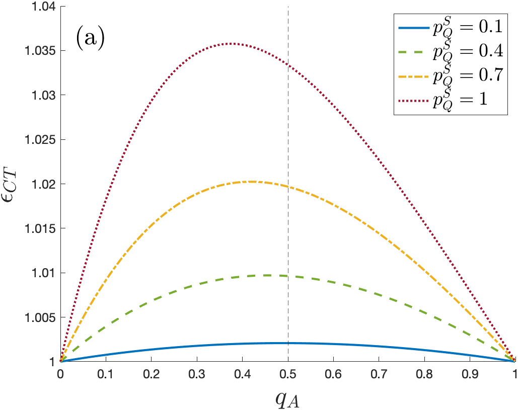
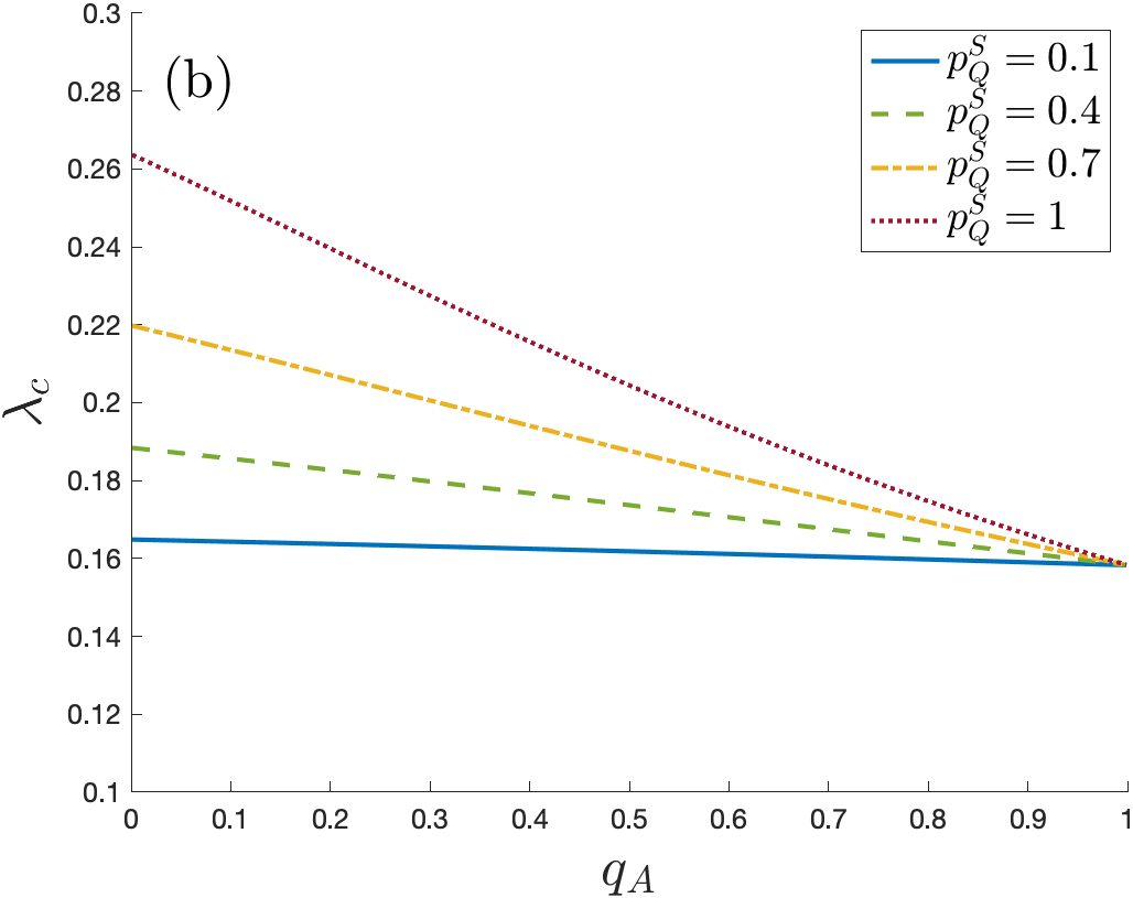
Figure 2: (a) Plot of the efficacy of CT $\epsilon_{CT}$ as a function of $q_{A}$ for various values of $p_{Q}^{S}$. (b) Plot of the threshold $\lambda_{c}$ against $q_{A}$ for the same parameters of panel (a). Parameter values: $\mu=\mu_{Q}=1$, $\mu_{U}=4$, $p_{Q}^{A}=p_{Q}^{S}$, $p_{CT}=1$, $\langle k\rangle=6.3$.

For instance, as a function of the share of fully asymptomatic infections, the efficacy of contact tracing attains a maximum (see Fig. 2(a)) for a value

$$q_{A}^{*} =\frac{(1+T_{U}/T)(1+T/T_{Q})-p_{Q}^{S}}{2(1+T_{U}/T)(1+T/T_{Q})-p_{Q}^{S}}$$

$$=\frac{1}{1+\lambda_{c}^{IDF}(q_{A}=0)}.$$ (5)

Interestingly, this value always falls in the range $q_{A}^{*}\in[0,1/2]$; it is a decreasing function of $p_{Q}^{S}$ and of the mean isolation period $T_{Q}$, while it grows with the delay to isolation $T_{U}$. Note however that, while a positive share of asymptomatic individuals $q_{A}^{*}>0$ may maximize the efficacy of contact tracing, it does not maximize the threshold (Eq. (2)), which reflects the combined efficacy of self-isolation of symptomatic individuals and quarantine of their asymptomatic contacts. Indeed, under the realistic assumption $p_{Q}^{A}\leq p_{Q}^{S}$, the epidemic threshold is always maximized by the complete absence of asymptomatic infections, $q_{A}=0$ (see Fig. 2(b)).

Plotting $\epsilon_{max}=\epsilon_{CT}(q_{A}^{*})$ as a function of $p_{Q}^{S}$ for various values of $T_{U}$ and $T_{Q}$ (Fig. 3) we find that, despite $\epsilon_{CT}$ assuming in principle values up to 2, the CT performance is much more limited: the contribution to the value of the epidemic threshold due to CT is in practice always of the order of a few percent.

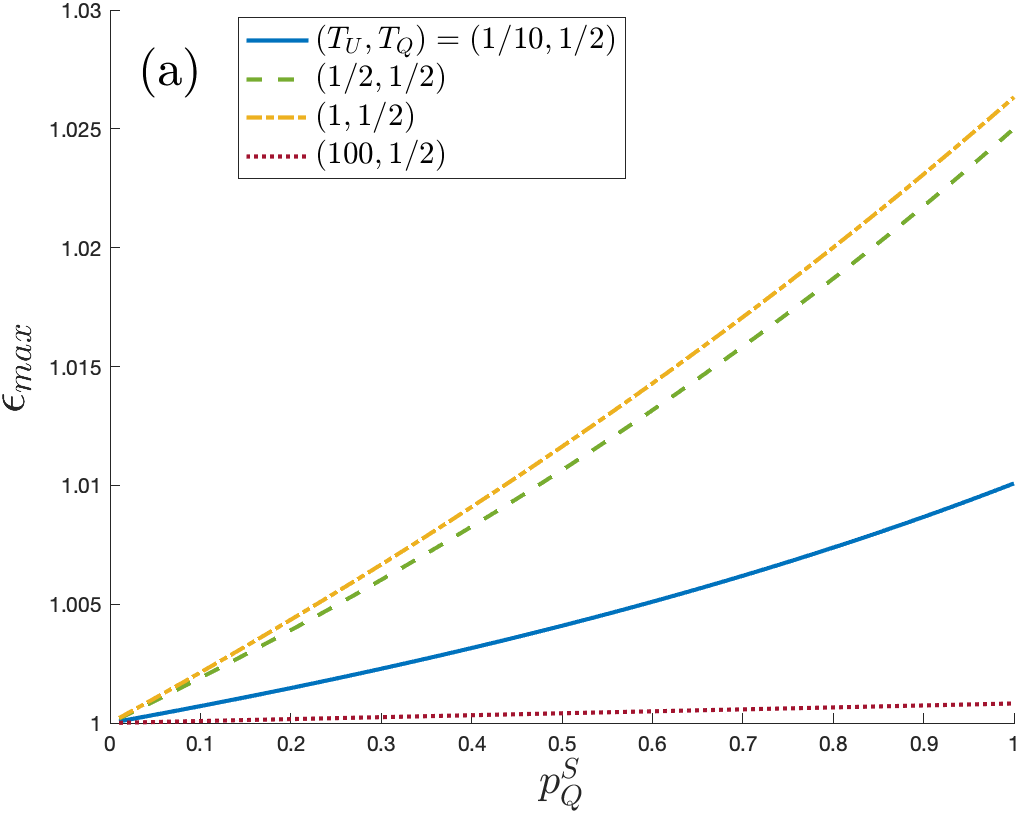
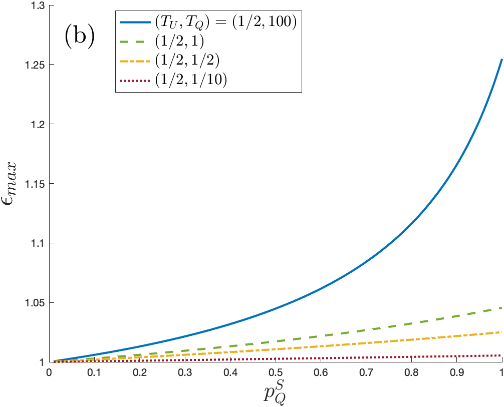
Figure 3: (a) Maximum value of $\epsilon_{CT}$ against $p_{Q}^{S}$ for (a) various values of $T_{U}$ ($T_{Q}=1/2$, $T=1$); (b) various values of $T_{Q}$ ($T_{U}=1/2$, $T=1$). We consider the case where $p_{CT}=1$.

Moreover, while $\lambda_{c}$ is maximised by $T_{U}\rightarrow 0$, from Eq. (4) we find that the efficacy of CT is maximized by a delay that can be positive, depending on the value of the other parameters

$$T_{U}^{*}=T\left(1-\frac{(1-q_{A})p_{Q}^{S}}{1+T/T_{Q}}\right),$$ (6)

but is nevertheless always shorter than the recovery time $T$ (see Fig. 4).

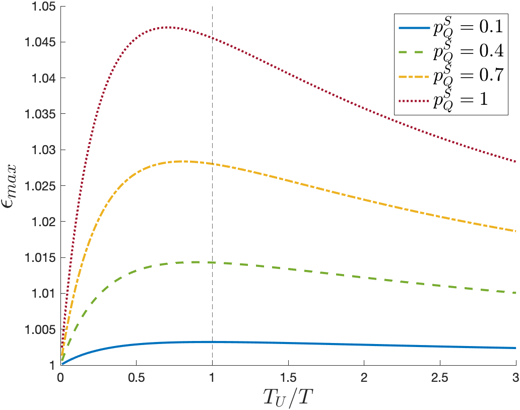
Figure 4: Plot of the maximum value of $\epsilon_{CT}$ against $T_{U}/T$ for various values of $p_{Q}^{S}$, showing the presence of a maximum. Parameter values: $T_{Q}=1$, $p_{CT}=1$.

This is a consequence of a nontrivial tradeoff between two competing effects. On the one hand, a short $T_{U}$ implies that essentially no asymptomatic is traced. On the other hand, for very long delays to isolation, many individuals are traced, but since they take a lot of time to quarantine they may infect many other individuals, thus reducing the effect of CT. Assuming that it is possible to act on all parameters, improvement of the efficacy of contact tracing is achieved when $T_{U},q_{A}\rightarrow 0$, $p_{Q}^{A},p_{Q}^{S},p_{CT}\rightarrow 1$, $T_{Q}\rightarrow\infty$.

In Appendix IX we present an analysis of the minimal values of the compliance $p_{Q}^{S}$ or $p_{Q}^{A}$ needed to eradicate an epidemic characterized by a given supercritical transmissibility $\lambda$.

III Prevalence in the endemic phase

This simple model for self-isolation and quarantine allows us also to analytically compute the stationary fractions of individuals in each compartment:

$$(U_{A}^{+})^{*} =\frac{q_{A}(1-q_{A})}{(1+T/T_{U})^{2}}p_{CT}\lambda_{c}\langle k\rangle\cdot\frac{\lambda-\lambda_{c}}{\lambda}$$ (7)

$$U_{S}^{*} =\frac{(1-q_{A})}{1+T/T_{U}}\cdot\frac{\lambda-\lambda_{c}}{\lambda}$$

$$Q^{*} =\frac{1}{\lambda\langle k\rangle}(1-\lambda_{c}\langle k\rangle+\lambda\langle k\rangle\times$$

$$\times\frac{1+ap_{Q}^{S}-\sqrt{(1-ap_{Q}^{S})^{2}-4\frac{a}{1+T/T_{U}}p_{CT}p_{Q}^{A}q_{A}}}{2})$$

$$F^{*} =\frac{T}{T_{Q}}Q^{*}$$

$$I^{*} =\frac{T}{T_{U}}(1-p_{Q}^{S})(U_{S})^{*}+\frac{T}{T_{U}}(1-p_{Q}^{A})(U_{A}^{+})^{*}$$

$$(U_{A}^{-})^{*} =(1+T/T_{U})[\frac{q_{A}}{1-q_{A}}U_{S}^{*}-(U_{A}^{+})^{*}],$$

where $a=\frac{(1-q_{A})}{(1+\frac{T_{U}}{T})(1+\frac{T}{T_{Q}})}$.

In the limit where $q_{A}\rightarrow 0$, we recover the prevalences of the IDF model de Meijere et al. (2021), where the fractions $(U_{A}^{+})^{*}$ and $(U_{A}^{-})^{*}$ vanish, while $U_{S}^{*}\rightarrow\frac{1}{1+T/T_{U}}\frac{\lambda-\lambda_{c}}{\lambda}$. In the same limit, the fraction of isolated and quarantined individuals reduces to $Q^{*}=\frac{p_{Q}^{S}}{(1+T/T_{Q})(1+T_{U}/T)}\frac{\lambda-\lambda_{c}}{\lambda}$.

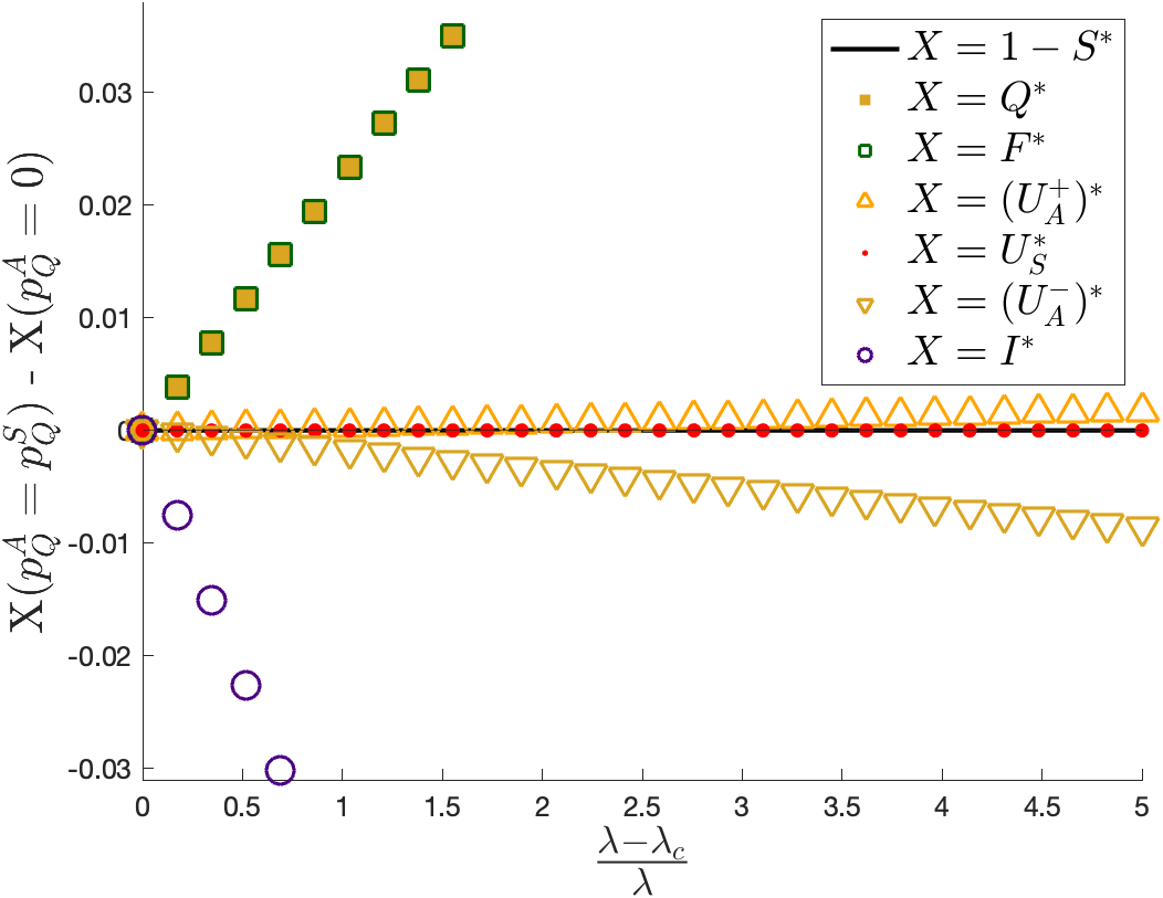
Figure 5: Plot of the difference between the stationary fractions of individuals with ($p_{Q}^{A}=p_{Q}^{S}=0.9$) and without ($p_{Q}^{A}=0$) CT, as a function of the distance $(\lambda-\lambda_{c})/\lambda$ from the threshold. Parameter values: $\mu=1$, $\mu_{U}=4$, $\mu_{Q}=1$, $q_{A}=0.5$, $p_{CT}=1$, $\langle k\rangle=6.3$.

Considering a virus transmissibility standing at a fixed distance $\frac{\lambda-\lambda_{c}}{\lambda}$ from the epidemic threshold we are able to compare the dependence on $p_{Q}^{A}$ of these stationary fractions of individuals above $\lambda_{c}$. At a fixed distance from the epidemic threshold, the stationary fraction of symptomatic individuals $U_{S}^{*}$ remains unaffected by changes in the compliance $p_{Q}^{A}$ of asymptomatic individuals. However, since the epidemic threshold is an increasing function of $p_{Q}^{A}$, $(U_{A}^{+})^{*}$ increases with $p_{Q}^{A}$ while $(U_{A}^{-})^{*}$ decreases. The quarantine of asymptomatic individuals therefore enhances the system’s tracing capacity. Having $U_{A}^{+}$ individuals transitioning to $Q$ instead of $I$ indeed reduces the chances of having infectors $I$ that do not trace their asymptomatic contacts. The total fraction of undecided individuals $(U_{A}^{+})^{*}+(U_{A}^{-})^{*}+U_{S}^{*}$ is expected overall to decrease, while the fractions of individuals in $Q$ and $F$ increase when asymptomatic compliance $p_{Q}^{A}$ increases.

This is supported by Fig. 5 where we see, for a given choice of the parameter values, the increasing or decreasing effect of $p_{Q}^{A}$ on the quasistationary values, at a given distance from the epidemic threshold. We consider the stationary fractions of individuals in a generic compartment $X$ when $p_{Q}^{A}=p_{Q}^{S}$ (contact tracing is maximally operative) and when $p_{Q}^{A}=0$ (contact tracing is not active), as functions of $(\lambda-\lambda_{c}(p_{Q}^{A}=p_{Q}^{S}))/\lambda$ and $(\lambda-\lambda_{c}(p_{Q}^{A}=0))/\lambda$, respectively. We then plot the difference between the stationary fractions of individuals in these limit cases, so that positive values indicate that the activation of contact tracing populates the corresponding compartment. We find that the amount by which $(U_{A}^{+})^{*}$ and $I^{*}$ decrease is perfectly balanced by the amount by which $Q^{*}$, $F^{*}$ and $(U_{A}^{-})^{*}$ increase, overall resulting in a fraction of infected individuals $Q^{*}+I_{tot}^{*}=1-S^{*}$ invariant under changes in adherence of asymptomatic individuals, at a fixed distance from the epidemic threshold.

At a fixed spreading rate, the shift of the epidemic threshold induced by the implementation of the contact tracing measure, reduces the distance of the system from the critical point, in the supercritical regime. This has the effect of making the system reach a lower stationary state (and also more slowly) than in the absence of contact tracing.

IV Numerical simulations

In order to check whether the results obtained in the mean-field setting also hold for the fully stochastic dynamics, we perform numerical simulations using a Gillespie optimized algorithm Cota and Ferreira (2017) to implement the SIS-like dynamics on networks built according to the uncorrelated configuration model Catanzaro et al. (2005). We consider power-law degree-distributed networks with exponent $\gamma$ and network size $N=10^{4}$. The node degrees are constrained in the range $k\in[k_{min}=3,k_{max}=\sqrt{N}]$ – in order to have an uncorrelated network without multiple and self connections. In this setting, we estimate the epidemic threshold by finding the value of $\lambda$ at which the susceptibility of the system reaches a maximum Ferreira et al. (2012). We implement the Quasistationary State method (QS) Ferreira et al. (2012), for which the dynamics never allows the system to reach the healthy absorbing state. We consider both homogeneous ($\gamma=10$) and strongly heterogeneous ($\gamma=2.5$) networks and compare the results with the mean-field theory.

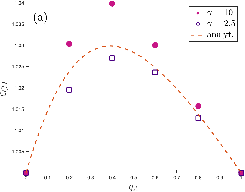
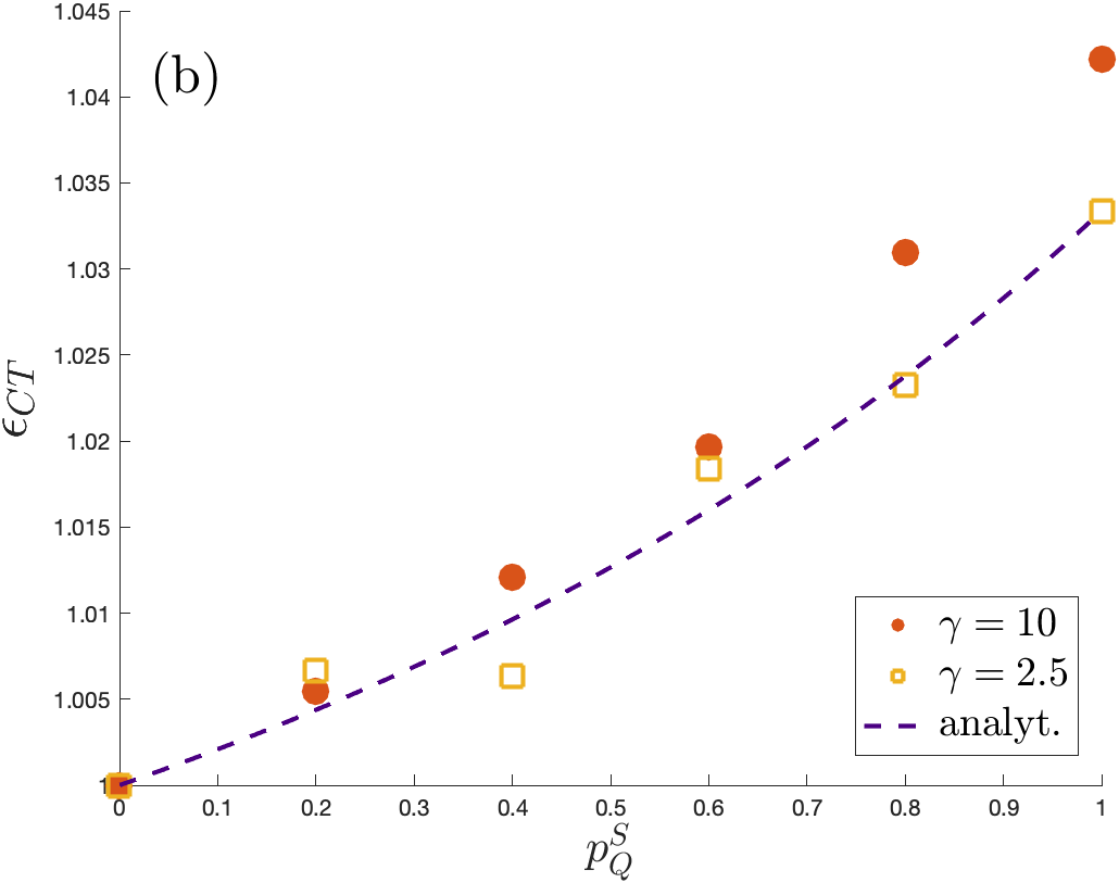
Figure 6: Efficacy of contact tracing in a homogeneous network ($\gamma=10$) and in a strongly heterogeneous network ($\gamma=2.5$) (analytical prediction, numerical estimates for both $\gamma=2.5$ and $\gamma=10$). (a) $\epsilon_{CT}$ as a function of $q_{A}$, with $p_{Q}^{S}=0.9$. (b) $\epsilon_{CT}$ as a function of $p_{Q}^{S}$, with $q_{A}=0.5$. Parameter values: $\mu=\mu_{Q}=1$, $\mu_{U}=4$, $p_{CT}=1$.

In Fig. 6 we show that there is a good agreement between numerical simulations and analytical results.

To perform numerical simulations one needs to specify how the symptomatic/asymptomatic status and the compliance to isolation/quarantine are chosen for each individual. To obtain the results presented in Fig. 6 we have assumed that the choice is annealed, in the sense that, for a given individual at each infection event, the development of an asymptomatic form of infection and the decision to isolate are drawn randomly with the corresponding probabilities. A possibly more realistic alternative is that the probability of developing an asymptomatic form of infection and the probability of self-isolating are individual-based. This corresponds to the quenched case, where a given individual always develops the same form of infection (whether symptomatic or asymptomatic) and always takes the same decision concerning isolation (whether it is to isolate or not to isolate). The immune history of individuals is indeed known to play a role in the probability of developing asymptomatic forms of infection Wang et al. (2023) while personal conditions and beliefs concerning self-isolation from the community likely determine compliance at an individual level Smith et al. (2020).

In Fig. 7 we compare the results we obtain in all possible scenarios of quenched or annealed treatment of the development of an asymptomatic form of infection and of the decision of isolating or not.

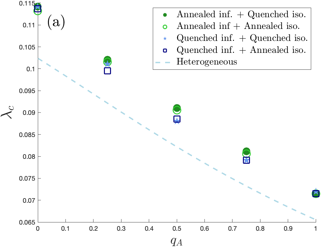
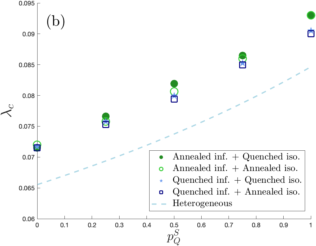
Figure 7: Role of quenchedness (numerical predictions and Heterogeneous mean-field estimates achieved by substituting the homogeneous mean-field topological factor $1/\langle k\rangle$ by $\langle k\rangle/\langle k^{2}\rangle$. (a) $\lambda_{c}$ vs $q_{A}$ for all quenched-annealed combinations, with $p_{Q}^{S}=0.9$. (b) $\lambda_{c}$ vs $p_{Q}^{S}$ for all quenched-annealed combinations, with $q_{A}=0.5$. Parameter values: $\mu=\mu_{Q}=1$, $\mu_{U}=4$, $p_{CT}=1$.

The figures show minimal differences between the various cases, even for a strongly heterogeneous degree distribution.

V A more realistic model for In-host Disease Progression

The stylized model we considered analytically does not only oversimplify the contact network, it also makes unrealistic assumptions concerning the way the disease progresses within infected individuals. In particular, the assumption that infection and recovery transitions are Poissonian and the constant infectiousness over the course of infection are unrealistic for the modelling of COVID-19. Moreover, the latent period during which newly infected individuals are not infectious yet and the pre-symptomatic period are not considered at all. These assumptions might strongly affect the efficacy of the contact tracing and case isolation measures. The model also neglects the fact that the contact tracing measure is able to isolate not only asymptomatic contacts but also symptomatic contacts in their pre-symptomatic phase.

In this section we check whether our conclusions on the efficacy of the contact tracing measure also hold in a much more complex and realistic model of disease progression. We consider the propagation of the Omicron variant of SARS-CoV-2 on the branching process model for disease propagation introduced in de Meijere et al. (2023). Such a model takes into account different transmissibilities for symptomatic and asymptomatic individuals, an evolution of infectiousness over the course of the infection (through a distribution of generation intervals) with a latent period, and a pre-symptomatic period (through a distribution of incubation periods). It also models different levels of immunity across the population (different numbers of doses of vaccine administered to each individual with a waning of protection against infection and symptomatic infection informed by available estimates for the Omicron variant), time varying test sensitivity (sensitivity of antigenic tests varying over the course of infection) and imperfect adherence to the measures (delay to isolation, partial contact reduction during the isolation period, imperfect share of successfully traced contacts, imperfect compliance to testing and to isolation, anticipated exit from isolation as a consequence of fatigue).

For a better comparison with our analytical results, we cancel the effects of heterogeneous immunity across the population (all individuals are equally susceptible to infection, all individuals being considered as unvaccinated), the effect of being asymptomatic on the potential to further transmit the disease (same transmissibility for symptomatic and asymptomatic individuals) and the role played by testing (perfect test sensitivity, perfect compliance and vanishing delay to testing). We fix our baseline parameters to conditions that favor the performance of CT: vanishing delay between information of being infected and isolation, perfect isolation from the community during the isolation period, long isolation duration (population mean of 11 days, i.e. 1.6 times the infectious period that we use as a proxy of the time for recovery), perfect tracing capacity, perfect compliance to recommendations in terms of isolation duration.

In order to have a quantitative measurement of the efficacy of contact tracing akin to our definition in the mean-field model, we take $\epsilon_{CT}$ as the ratio between two “critical” basic reproduction numbers, determined in the case asymptomatic compliance to isolation is maximum ($p_{Q}^{A}=p_{Q}^{S}$) and in the case where it is minimum ($p_{Q}^{A}=0$). The “critical” basic reproduction number for a given set of parameters is the initial value of $R_{0}$ that generates an effective reproduction number $R_{\textrm{eff}}=1$, when interventions (self-isolation and/or CT) are implemented.

In Fig. 8 we compare the maximum efficacy (as a function of $q_{A}$) of the contact tracing measure as computed within our mean-field model and as estimated through the branching process model. We approximate the time between infection and information of being infected with the mean incubation period of the branching process model. Disregarding the delay between information of being infected and isolation, this implies a ratio $T_{U}/T=0.49$ between the delay from infection to isolation (approximated by the mean incubation period of 3.48 days) and the time for recovery (approximated by the mean infectious period of 7.04 days). The figure shows that even a complex and realistic in-host disease progression model predicts a limited efficacy of the contact tracing measure. Even in extremely favorable conditions, the increase of the epidemic threshold remains smaller than $25\%$, in line with our SIS-based compartmental model.

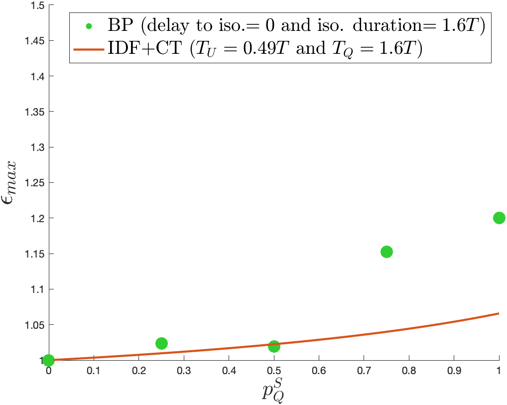
Figure 8: Comparison between estimates of the maximum efficacy (as a function of $p_{Q}^{S}$) of the contact tracing measure in the branching process model of de Meijere et al. (2023) and in our compartmental model (recovery time $T=1$ and tracing capacity $p_{CT}=1$). “delay to iso.” in the BP model refers to the delay between information of infection and isolation.

VI Conclusions

In this work we developed an SIS-based epidemic model for self-isolation and (forward and first-order) contact tracing measures in the presence of imperfect compliance and delays. We find that the quarantine of asymptomatic contacts has a very limited impact on increasing the epidemic threshold. Moreover, it only decreases the total fraction of infected individuals through the achieved increase of the epidemic threshold. It is however especially useful to quarantine asymptomatic patients in case of outbreaks caused by viruses that generate low to intermediate shares of asymptomatic infections, and that propagate in populations where behavioral and logistical delays to isolation are smaller but close to the time for recovery. We find that it is always crucial to incentivate adherence to isolation, especially for symptomatic individuals.

These conclusions are supported by analytical results in a homogeneous mean-field setting, allowing for an explicit characterization of the interplay between disease properties and behavioral conditions. The role of more realistic contact network characteristics and more complex in-host disease progression, involving for instance delayed onset of symptoms is investigated too, with overall conclusions remaining unaffected.

In SIR-like models, the duration of an outbreak and the height of the peak of the fraction of infected individuals are very important observables and the efficacy of CT can be measured by the reduction in their values. In the present SIS-like model, these observables are not defined. The effect of CT on the temporal evolution is given here by the increase of the temporal scale $\tau$ governing the initial exponential growth of the epidemic. Since $\tau\propto 1/(\lambda-\lambda_{c})$, the effect of CT can be ascribed to the increase of the threshold.

In this study we have only considered the effect of forward contact tracing, as the tracing process allows the quarantine of asymptomatic individuals who have been in contact with a symptomatic infector. Backward contact tracing, i.e. the search for the asymptomatic infector of the symptomatic index case, with the goal of quarantining him/her and thus preventing further spreading, is known to be highly effective, in particular in heterogeneous networks Kojaku et al. (2021). It would be interesting to check how the results presented here are modified if also backward contact tracing is in place. A different model where both types of CT are at work indicates that in such a case contact tracing may lead to a stronger increase of the epidemic threshold Mancastroppa et al. (2021). Our model also does not study the tracing of susceptible contacts of index cases (which would represent an interesting quantity to measure the social weight of the intervention) nor the tracing of infected contacts that were not infected by the index case. A model by Lee et al. Lee et al. (2022) focuses on these two aspects of CT, which however do not change the value of the epidemic threshold. Indeed, the former does not isolate infected individuals and the latter necessitates the contact between two infected individuals that becomes irrelevant near the disease-free equilibrium.

The present study focuses on a population with homogeneous infection rates, thus neglecting heterogeneities in immune history (whether provided by previous infections or vaccination) and in age-related immune response. Moreover, the possibility of correlations among individuals with respect to biological and/or behavioral features is disregarded. The existence of clustering in the contact network has been neglected as well. While containment measures such as vaccination and CT are expected to suffer from assortativity in adherence Glaubitz and Fu (2022); Rizi et al. (2022), at least in some regimes Burgio et al. (2021), the contact tracing measure is predicted to benefit from clustering House and Keeling (2010); Burdinski et al. (2022); Kiss et al. (2005). Finally, we make a set of assumptions that might lead to overestimates of the efficacy of the contact tracing measure. Our model neglects the role of diagnostic tests, massively used during the COVID-19 pandemic. It does not distinguish between the intrinsic transmissibilities of asymptomatic and symptomatic individuals. Even symptomatic individuals who do not comply with isolation trace their contacts, which is not realistic. We moreover assume immediate tracing of contacts upon infection.

The analysis of modifications of the current framework, where one or more of these simplyfing assumptions are lifted, constitutes an interesting avenue for further research.

VII List of Transitions

• Spontaneous decays to $S$

  Transition Rate

  $$I\to S \mu$$

  $$U_{S}\to S \mu$$

  $$U_{A}^{+}\to S \mu$$

  $$U_{A}^{-}\to S \mu$$

  $$Q\to S \mu$$

  $$F\to S \mu$$

• Spontaneous decays to $F$

  Transition Rate

  $$Q\to F \mu_{Q}$$

• Transitions from Undecided states

  Transition Rate

  $$U_{S}\to Q \mu_{U}p_{Q}^{S}$$

  $$U_{S}\to I \mu_{U}(1-p_{Q}^{S})$$

  $$U_{A}^{+}\to Q \mu_{U}p_{Q}^{A}$$

  $$U_{A}^{+}\to I \mu_{U}(1-p_{Q}^{A})$$

• Infections by $U_{S}$ nodes

  Transition Rate

  $$S+U_{S}\to U_{A}^{+}+U_{S} \beta q_{A}p_{CT}$$

  $$S+U_{S}\to U_{A}^{-}+U_{S} \beta q_{A}(1-p_{CT})$$

  $$S+U_{S}\to U_{S}+U_{S} \beta(1-q_{A})$$

• Infections by $X=(U_{A}^{+},U_{A}^{-},I,F)$ nodes

  Transition Rate

  $$S+X\to U_{A}^{-}+X \beta q_{A}$$

  $$S+X\to U_{S}+X \beta(1-q_{A})$$

VIII Demonstration that the threshold $\lambda_{c}$ is always real

We want to show that $\chi\leq 1/2$. Let us start from the more restrictive condition $\chi\leq p_{CT}p_{Q}^{A}/2$, which can be written as a second order inequality for $q_{A}$:

$$q_{A}^{2} \left[(p_{Q}^{S})^{2}+4\frac{T_{U}}{TT_{Q}}(T+T_{Q})\right]+$$

$$q_{A}\left[2p_{Q}^{S}\left(\frac{T}{T_{Q}}+\frac{T_{U}}{T}+\frac{T_{U}}{T_{Q}}\right)-4\frac{T_{U}}{TT_{Q}}(T+T_{Q})\right]+$$

$$\left(\frac{T}{T_{Q}}+\frac{T_{U}}{T}+\frac{T_{U}}{T_{Q}}\right)^{2}\geq 0.$$ (8)

We now show that this condition holds for any $q_{A}\in[0,1]$.

The minimum of the left hand side of Eq. (8) (L.H.S.) is always located at values of $q_{A}<1$. Indeed,

$$\text{argmin}_{q_{A}}L.H.S. <1$$

$$-2\frac{T_{U}}{TT_{Q}}(T+T_{Q})-(p_{Q}^{S})^{2} -p_{Q}^{S}(\frac{T}{T_{Q}}+\frac{T_{U}}{T}+\frac{T_{U}}{T_{Q}})<0,$$ (9)

which is always true.

The condition for the minimum of the L.H.S. to be located at $q_{A}>0$ is

$$\text{argmin}_{q_{A}}L.H.S. >0$$

$$p_{Q}^{S} <\frac{2T_{U}(T+T_{Q})}{T^{2}+T_{U}(T+T_{Q})}.$$ (10)

Hence it depends on $p_{Q}^{S}$ whether the minimum is for $q_{A}$ smaller or larger than zero.

In the first case, Eq. (8) is always satisfied between $q_{A}=0$ and $q_{A}=1$, because it is already true for $q_{A}=0$ and the L.H.S. is a growing function of $q_{A}$.

In the other case, Eq. (8) is always satisfied because it is satisfied in the minimum. Indeed, the minimum of the L.H.S. is positive if the following condition on the parameters holds:

$$\left(\frac{T}{T_{Q}}+\frac{T_{U}}{T}+\frac{T_{U}}{T_{Q}}\right)^{2}$$

$$\geq\frac{T_{U}}{TT_{Q}}(T+T_{Q})-p_{Q}^{S}\left(\frac{T}{T_{Q}}+\frac{T_{U}}{T}+\frac{T_{U}}{T_{Q}}\right).$$ (11)

Under the assumption of $\text{argmin}_{q_{A}}L.H.S.>0$ (using Eq. (10)), we find that it is always true because:

$$\left(\frac{T}{T_{Q}}+\frac{T_{U}}{T}+\frac{T_{U}}{T_{Q}}\right)^{2}\geq$$

$$>\frac{T_{U}}{TT_{Q}}(T+T_{Q})-\frac{2T_{U}(T+T_{Q})}{T^{2}+T_{U}(T+T_{Q})}\left(\frac{T}{T_{Q}}+\frac{T_{U}}{T}+\frac{T_{U}}{T_{Q}}\right)$$ (12)

$$=\frac{T_{U}}{TT_{Q}}(T+T_{Q})-2\frac{T_{U}}{TT_{Q}}(T+T_{Q})$$ (13)

$$=-\frac{T_{U}}{TT_{Q}}(T+T_{Q}).$$

We conclude that the condition $\chi\leq p_{CT}p_{Q}^{A}/2$ is always met in the interval $q_{A}\in[0,1]$. When $\text{argmin}_{q_{A}}L.H.S.<0$, the L.H.S. is positive in the interval $q_{A}\in[0,1]$ and when $\text{argmin}_{q_{A}}L.H.S.>0$, we have $\text{min}(L.H.S.)>0$ implying too that $\chi\leq p_{CT}p_{Q}^{A}/2$. Since $p_{Q}^{A},p_{CT}\in[0,1]$, $\chi\leq 1/2$ and the epidemic threshold is real.

IX Critical compliance

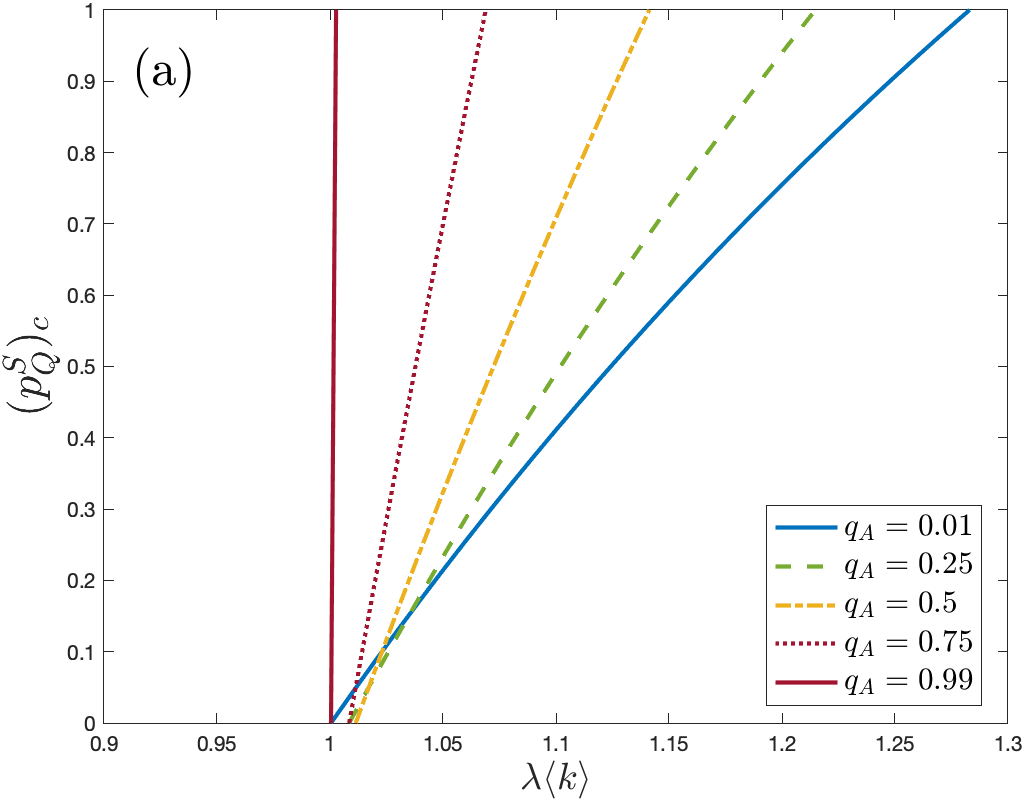
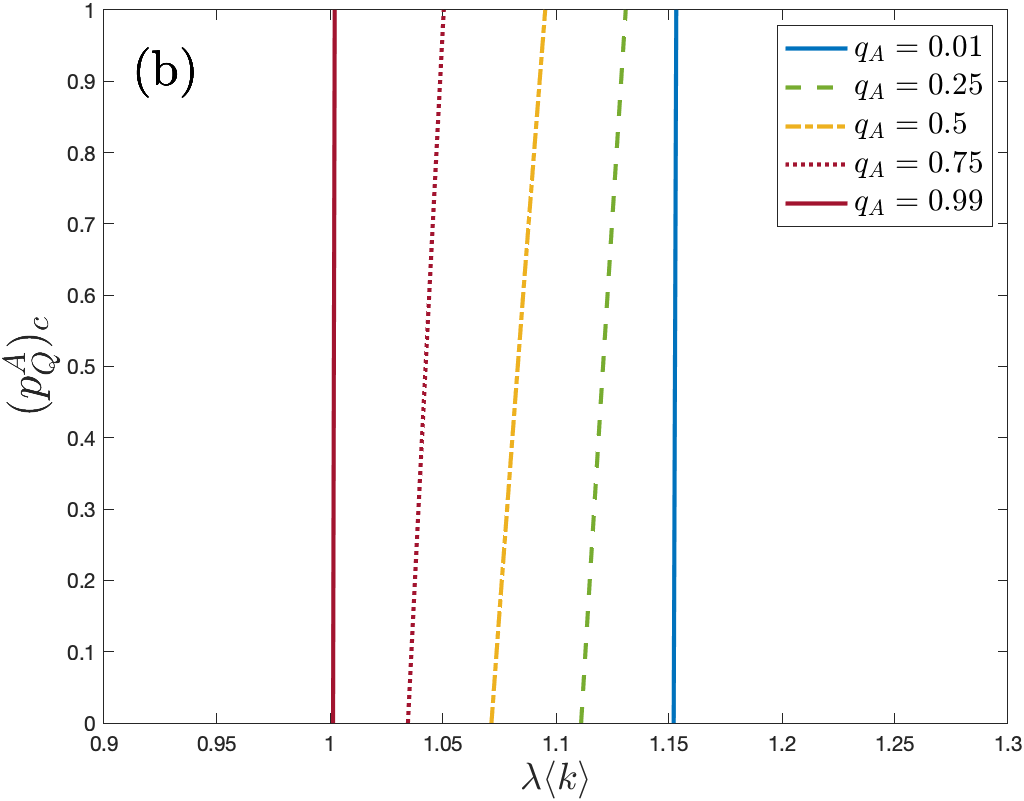
Figure 9: (a) Critical value of the compliance probability of symptomatic individuals against $\lambda\langle k\rangle$ for various values of asymptomatic probability $q_{A}\in[0,1]$ ($p_{Q}^{A}=0.6$). (b) Critical value of the compliance probability of asymptomatic individuals against $\lambda\langle k\rangle$ for various values of asymptomatic probability $q_{A}\in[0,1]$ ($p_{Q}^{S}=0.6$). Parameter values: $\mu=1$, $\mu_{U}=\mu_{Q}=2$.

In this appendix we study the role of the compliance of symptomatic and asymptomatic individuals in containing the spread of the epidemic. Given a pathogen with a specific value of $\lambda$, what are the values of $p_{Q}^{S}$ that are sufficient to make $\lambda<\lambda_{c}$ so that the epidemic becomes subcritical and disappears?

Setting $\lambda=\lambda_{c}$ and inverting Eq. (2), the expression of $p_{Q}^{S}$ that allows the system to reach the epidemic threshold is easily derived

$$(p_{Q}^{S})_{c}=\left[1-\frac{\chi(\lambda/\lambda_{c}^{IDF}(q_{A}))^{2}+2}{2(\lambda\langle k\rangle)}\right]\frac{(1+T_{U}/T)(1+T/T_{Q})}{1-q_{A}}.$$ (14)

This expression for $(p_{Q}^{S})_{c}$ is not a priori limited to the $[0,1]$ interval. Values of $(p_{Q}^{S})_{c}<0$ imply that the system does not require isolation of symptomatic individuals to reach the epidemic threshold. In practice this means that $\lambda$ is already subcritical in the absence of isolation of symptomatic individuals. Values $(p_{Q}^{S})_{c}>1$ mean instead that even the isolation of all symptomatic individuals is not sufficient to drive the system to the disease-free state.

These results can be translated into ranges of values of the virus transmissibility $\lambda\langle k\rangle$ that the isolation of symptomatic individuals is able to contain. Isolation of symptomatic individuals is not necessary when

$$\lambda\langle k\rangle \leq\lambda_{c}^{IDF+CT}(q_{A})|_{p_{Q}^{S}=0}\langle k\rangle$$ (15)

$$=\frac{1-\sqrt{1-2\chi}}{\chi},$$ (16)

as the outbreak would be contained regardless of their isolation. On the other hand, thanks to the isolation of symptomatic individuals, the outbreak can be contained for values of the transmissibility rate $\lambda\langle k\rangle$ larger than the SIS result but as long as

$$\lambda\langle k\rangle \leq\lambda_{c}^{IDF+CT}(q_{A})|_{p_{Q}^{S}=1}\langle k\rangle$$ (17)

$$=\frac{1}{1-a}\cdot\frac{1-\sqrt{1-2\chi}}{\chi},$$ (18)

where $a=\frac{(1-q_{A})}{(1+\frac{T_{U}}{T})(1+\frac{T}{T_{Q}})}$.

In Fig. 9(a) we plot the dependence of $(p_{Q}^{S})_{c}$ on $\lambda\langle k\rangle$ for various values of the probability $q_{A}$ of being asymptomatic. We see that the isolation of symptomatic individuals is the more useful to contain the spread of more transmissible infectious pathogens the lower the share of asymptomatic individuals in the infected population.

We repeat the above reasoning with the compliance $p_{Q}^{A}$ of asymptomatic individuals with isolation mandates. The critical value of $p_{Q}^{A}$ that allows to reach the epidemic threshold is

$$(p_{Q}^{A})_{c} =\frac{1}{\delta}\frac{1}{\lambda\langle k\rangle}\left[\frac{1}{\lambda^{IDF}(q_{A})\langle k\rangle}-\frac{1}{\lambda\langle k\rangle}\right],$$ (19)

where $\delta=\frac{q_{A}(1-q_{A})p_{CT}}{(1+\frac{T}{T_{U}})(1+\frac{T_{U}}{T})(1+\frac{T}{T_{Q}})}$.

The outbreak can be contained by quarantining traced asymptomatics if

$$\lambda_{c}^{IDF+CT}(q_{A})|_{p_{Q}^{A}=0}\leq\lambda\leq\lambda_{c}^{IDF+CT}(q_{A})|_{p_{Q}^{A}=1}$$ (20)

$$\frac{1}{1-ap_{Q}^{S}}\leq\lambda\leq\frac{1}{1-ap_{Q}^{S}}\frac{1-\sqrt{1-2\chi(p_{Q}^{A}=1)}}{\chi(p_{Q}^{A}=1)}.$$ (21)

In Fig. 9(b) we show the dependence of the critical value of $p_{Q}^{A}$ on $\lambda\langle k\rangle$ for various values of $q_{A}\in[0,1]$. A comparison with panel (a) of the same figure shows that for the chosen values of the parameters, the role played by the isolation of symptomatic individuals is significantly larger than the one played by the quarantine of asymptomatic individuals.

References

- Fraser et al. (2004) C. Fraser, S. Rilley, R. M. Anderson, and N. M. Ferguson, PNAS 101, 6146 (2004).
- Ferretti et al. (2020) L. Ferretti, C. Wymant, M. Kendall, L. Zhao, A. Nurtay, L. Abeler-Dörner, M. Parker, D. Bonsall, and C. Fraser, Science 368 (2020), https://doi.org/10.1126/science.abb6936.
- Johansson et al. (2021) M. A. Johansson, T. M. Quandelacy, S. Kada, P. V. Prasad, M. Steele, J. T. Brooks, R. B. Slayton, M. Biggerstaff, and J. C. Butler, JAMA Network Open 4, e2035057 (2021).
- Li et al. (2020) R. Li, S. Pei, B. Chen, Y. Song, T. Zhang, W. Yang, and J. Shaman, Science 368, 489 (2020).
- Groendyke and Combs (2021) C. Groendyke and A. Combs, Epidemiologic Methods 10, 20200030 (2021).
- Riley et al. (2003) S. Riley, C. Fraser, C. A. Donnelly, A. C. Ghani, L. J. Abu-Raddad, A. J. Hedley, G. M. Leung, L.-M. Ho, T.-H. Lam, T. Q. Thach, et al., Science 300, 1961 (2003).
- Lipsitch et al. (2003) M. Lipsitch, T. Cohen, B. Cooper, J. M. Robins, S. Ma, L. James, G. Gopalakrishna, S. K. Chew, C. C. Tan, M. H. Samore, et al., science 300, 1966 (2003).
- Ferguson et al. (2001) N. M. Ferguson, C. A. Donnelly, and R. M. Anderson, Nature 413, 542 (2001).
- Foege et al. (1971) W. H. Foege, J. D. Millar, and J. M. Lane, American journal of epidemiology 94, 311 (1971).
- Riley and Ferguson (2006) S. Riley and N. M. Ferguson, Proceedings of the National Academy of Sciences 103, 12637 (2006).
- Fox et al. (2013) G. J. Fox, S. E. Barry, W. J. Britton, and G. B. Marks, European Respiratory Journal 41, 140 (2013).
- Rutherford and Woo (1988) G. W. Rutherford and J. M. Woo, JAMA 259, 3609 (1988).
- Saurabh and Prateek (2017) S. Saurabh and S. Prateek, African health sciences 17, 225 (2017).
- Swanson et al. (2018) K. C. Swanson, C. Altare, C. S. Wesseh, T. Nyenswah, T. Ahmed, N. Eyal, E. L. Hamblion, J. Lessler, D. H. Peters, and M. Altmann, PLoS neglected tropical diseases 12, e0006762 (2018).
- Shin et al. (2020) Y. Shin, B. Berkowitz, and M. J. Kim, Washington Post 12 (2020).
- Silva and Martin (2020) C. Silva and M. Martin, “U.s. surgeon general blames ’pandemic fatigue’ for recent covid-19 surge,” https://www.npr.org/sections/coronavirus-live-updates/2020/11/14/934986232/u-s-surgeon-general-blames-pandemic-fatigue-for-recent-covid-19-surge?t=1619011823724 (2020).
- Gibney (2020) E. Gibney, Nature 581, 15 (2020).
- Blakely et al. (2020) T. Blakely, J. Thompson, N. Carvalho, L. Bablani, N. Wilson, and M. Stevenson, Medical Journal of Australia 213, 349 (2020).
- Knapton (2020) S. Knapton, “At least 11 countries have reimposed restrictions amid fears of coronavirus second wave,” (2020).
- Mancastroppa et al. (2021) M. Mancastroppa, C. Castellano, A. Vezzani, and R. Burioni, Nat. Commun. 12, 1919 (2021).
- Kerr et al. (2021) C. C. Kerr, D. Mistry, R. M. Stuart, K. Rosenfeld, G. R. Hart, R. C. Nùñez, J. A. Cohen, P. Selvaraj, R. G. Abeysuriya, M. Jastrz\kebski, L. George, B. Hagedorn, J. Panovska-Griffiths, M. Fagalde, J. Duchin, M. Famulare, and D. J. Klein, Nature Communications 12, 2993 (2021).
- Burdinski et al. (2022) A. Burdinski, D. Brockmann, and B. F. Maier, PLOS Digital Health 1, e0000149 (2022).
- Hellewell et al. (2020) J. Hellewell, S. Abbott, A. Gimma, N. I. Bosse, C. I. Jarvis, T. W. Russell, J. D. Munday, A. J. Kucharski, W. J. Edmunds, Centre for the Mathematical Modelling of Infectious Diseases COVID-19 Working Group, S. Funk, and R. M. Eggo, The Lancet Global Health 8, e488 (2020).
- Hasegawa and Nemoto (2017) T. Hasegawa and K. Nemoto, Physical Review E 96 (2017), 10.1103/PhysRevE.96.022311.
- Horstmeyer et al. (2022) L. Horstmeyer, C. Kuehn, and S. Thurner, Bulletin of mathematical biology 84 (2022), https://doi.org/10.1007/s11538-022-01033-3.
- Lee et al. (2022) D.-S. Lee, T.-Z. Liu, R. Zhang, and C.-S. Chang, ArXiv (2022), https://doi.org/10.48550/arXiv.2212.09093.
- Heidecke et al. (2022) J. Heidecke, J. Fuhrmann, and M. V. Barbarossa, ArXiv (2022), https://doi.org/10.48550/arXiv.2207.09551.
- House and Keeling (2010) T. House and M. J. Keeling, PLOS Computational Biology 6, e1000721 (2010).
- Reyna-Lara et al. (2021) A. Reyna-Lara, D. Soriano-Paños, S. Gómez, C. Granell, J. T. Matamalas, B. Steinegger, A. Arenas, and J. Gómez-Gardeñez, Physical Review Research 3 (2021), 10.1103/PhysRevResearch.3.013163.
- Bianconi et al. (2021) G. Bianconi, H. Sun, G. Rapisardi, and A. Arenas, Physical Review Research 3 (2021), 10.1103/PhysRevResearch.3.L012014.
- Kojaku et al. (2021) S. Kojaku, L. Hébert-Dufresne, E. Mones, S. Lehmann, and Y.-Y. Ahn, Nature Physics 17, 652 (2021).
- Burgio et al. (2021) G. Burgio, B. Steinegger, G. Rapisardi, and A. Arenas, Physical Review E 3 (2021), 10.1103/PhysRevResearch.3.033128.
- Rizi et al. (2022) A. K. Rizi, A. Faqeeh, A. Badie-Modiri, and M. Kivelä, Physical Review E 105, 044313 (2022).
- Kiss et al. (2005) I. Z. Kiss, D. M. Green, and R. R. Kao, Proceedings of the Royal Society - Biological Sciences 272, 1407 (2005).
- de Meijere et al. (2021) G. de Meijere, V. Colizza, E. Valdano, and C. Castellano, Physical Review E 104 (2021), https://doi.org/10.1103/PhysRevE.104.044316.
- Cota and Ferreira (2017) W. Cota and S. C. Ferreira, Computer Physics Communications 219, 303 (2017).
- Catanzaro et al. (2005) M. Catanzaro, M. Boguñá, and R. Pastor-Satorras, Phys. Rev. E 71 (2005), 10.1103/PhysRevE.71.027103.
- Ferreira et al. (2012) S. C. Ferreira, C. Castellano, and R. Pastor-Satorras, Phys. Rev. E 86 (2012), 10.1103/PhysRevE.86.041125.
- Wang et al. (2023) B. Wang, P. Andraweera, S. Elliott, H. Mohammed, Z. Lassi, A. Twigger, C. Borgas, S. Gunasekera, S. Ladhani, and H. S. Marshall, The Pediatric Infectious Disease Journal 42, 232 (2023).
- Smith et al. (2020) L. E. Smith, R. Amlôt, H. Lambert, I. Oliver, C. Robin, L. Yardley, and G. J. Rubin, Public Health 187, 41 (2020).
- de Meijere et al. (2023) G. de Meijere, E. Valdano, C. Castellano, M. Debin, C. Kengne-Kuetche, C. Turbelin, H. Noël, J. S. Weitz, D. Paolotti, L. Hermans, N. Hens, and V. Colizza, The Lancet Regional Health - Europe 28, 100614 (2023).
- Glaubitz and Fu (2022) A. Glaubitz and F. Fu, ArXiv (2022), https://doi.org/10.48550/arXiv.2212.13951.