Data-Driven Cooperative Adaptive Cruise Control for Unknown Nonlinear Vehicle Platoons

Abstract

This paper studies cooperative adaptive cruise control (CACC) for vehicle platoons with consideration of the unknown nonlinear vehicle dynamics that are normally ignored in the literature. A unified data-driven CACC design is proposed for platoons of pure automated vehicles (AVs) or of mixed AVs and human-driven vehicles (HVs). The CACC leverages online-collected sufficient data samples of vehicle accelerations, spacing and relative velocities. The data-driven control design is formulated as a semidefinite program (SDP) that can be solved efficiently using off-the-shelf solvers. The efficacy and advantage of the proposed CACC are demonstrated through a comparison with the classic adaptive cruise control (ACC) method on a platoon of pure AVs and a mixed platoon under a representative aggressive driving profile.

I Introduction

Vehicle platoon refers to a convoy of vehicles that travel at the same (longitudinal) velocity whilst maintaining a desired inter-vehicular distance. Previous studies [1, 2, 3] revealed that vehicle platoons have a great potential in reducing traffic congestion, accidents and fuel consumption. An effective control strategy is the key to establish vehicle platoons and has attracted much research attention.

The classic adaptive cruise control (ACC) [4], which has been well-developed and available on the market, enables the ego vehicle to follow its preceding vehicle. But ACC is not sufficient to establish a stable vehicle platoon [5, 6]. This motivated the development of a more advanced platooning control strategy, the cooperative adaptive cruise control (CACC), by using vehicle information shared in the platoon through vehicle-to-vehicle (V2V) wireless communications. Many works have shown that CACC can effectively establish stable platoons with pure automated vehicles (AVs) [7, 8]. Several works [9, 10, 11, 12] have shown that CACC are still effective for a more challenging case when a platoon has mixed AVs and human-driven vehicles (HVs), where the car-following behaviours of HVs are known to be different.

However, most existing CACC approaches hinge on linear vehicle models (i.e. the point-mass model) without considering the nonlinear dynamics. The nonlinear dynamics could be neglected for small-size passenger cars at low speeds but not for medium-size or large-size vehicles such as trucks and heavy-duty vehicles [13]. This limits the practical applicability of existing CACC designs in real traffic systems. Some works have studied CACC for nonlinear vehicle platoons through feedback linearisation based on accurately known vehicle parameters [14, 15, 13]. However, some vehicle parameters may be changing or unknown for CACC design. Another realistic concern is that in the heterogeneous platoon the parameters of other vehicles may be unknown to the ego AV. These make it necessary to develop CACC for platoons with unknown nonlinear vehicle dynamics.

Data-driven CACC that do not rely on the known vehicle dynamics have been recently developed for mixed vehicle platoons, using the methods like adaptive dynamic programming (ADP) [16, 17, 18], data-driven model predictive control (MPC) [12, 19], or reinforcement learning [20]. These methods are only applied to mixed platoons with linearised vehicle models. The CACC designs for pure AVs with nonlinear vehicle models were achieved by combining model-based control with linearisation of the nonlinear dynamics based on a parameter estimation [21] or data-driven feedforward control [22].

This paper proposes a novel data-driven CACC to address unknown nonlinear vehicle dynamics. The design takes inspiration from [23, 24] to represent the unknown platoon dynamics as a polynomial system. The main contributions are summarised as follows:

1. A strategy is developed for learning a nonlinear CACC controller from vehicle data samples through solving a semidefinite program (SDP).

2. The obtained CACC ensures the $H_{\infty}$ robust performance of the platoon against disturbances such as air/mechanical drags and reference velocity changes. In the data-driven control literature, $H_{\infty}$ robustness is either not addressed [24] or studied using sum-of-squares optimisation [23].

3. The proposed strategy is applicable to both pure AVs platoons and mixed platoons.

The rest of this paper is structured as follows. Section II describes the platoon model, Section III presents the data-driven CACC design for pure AVs and Section IV applies it to mixed platoons, Section V reports the simulation results, and Section VI draws the conclusions.

Notations: The interval $[a,b]$ is the set of integers from $a$ to $b$. $\mathrm{diag}(V_{1},\cdots,V_{n})$ denotes a block diagonal matrix with the main diagonals $V_{1},\cdots,V_{2}$. $I_{n}$ is a $n\times n$ identity matrix, $\mathbf{1}_{n}$ is a column of $n$ ones, and $\mathbf{0}$ is a zero matrix whose dimension is omitted unless necessary to be given.

II Platoon Modelling and Preliminaries

This paper considers a platoon with $n$ AVs equipped with V2V wireless communication devices. As in the literature, the design focuses on controlling the longitudinal dynamics of AVs to establish a platoon. To this end, a platooning error system needs to be built. The longitudinal dynamics of the $i$-th AV, $i\in[1,n]$, can be characterised by [14]:

$$\begin{split}\dot{p}_{i}&=v_{i},\\ \dot{v}_{i}&=a_{i},\\ \dot{a}_{i}&=f_{i}(v_{i},a_{i})+u_{i}/(\tau_{i}m_{i}),\end{split}$$ (1)

where $p_{i}$, $v_{i}$, and $u_{i}$ are the vehicle position, velocity, and control effort, respectively. $f_{i}(v_{i},a_{i})=-(a_{i}+R_{i}v_{i}^{2}+d_{i}/m_{i})/\tau_{i}-2R_{i}v_{i}a_{i}.$ $R_{i}=\sigma_{i}M_{i}c_{i}/(2m_{i})$ is the air resistance. $\tau_{i}$, $\sigma_{i}$, $M_{i}$, $c_{i}$, $d_{i}$, and $m_{i}$ are the engine time constant, specific mass of the air, cross-sectional area, drag coefficient, mechanical drag, and mass of the vehicle, respectively.

To facilitate the platooning control design, the nonlinear model (1) is commonly linearised in the literature (see e.g., [14, 15, 13]) using the feedback linearisation control law

$$u_{i}=m_{i}\bar{u}_{i}+0.5\sigma M_{i}c_{i}v_{i}^{2}+d_{i}+\tau_{i}\sigma M_{i}c_{i}v_{i}a_{i},$$ (2)

where $\bar{u}_{i}$ is the new control signal to be designed. However, (2) is applicable only when all the vehicle parameters $\tau_{i}$, $\sigma_{i}$, $M_{i}$, $c_{i}$, $d_{i}$ and $m_{i}$ are known. This is practically restrictive or even unrealistic because the parameters change with the driving environments such as payload, road conditions, weather, etc. It thus motivates us to develop a data-driven CACC for (1) with unknown $\tau_{i}$, $\sigma_{i}$, $M_{i}$, $c_{i}$, $d_{i}$ and $m_{i}$.

This paper aims to design $u_{i}$ for each AV to drive at a given desired constant velocity $v^{*}>0$ whilst maintaining a desired inter-vehicular distance $h^{*}>0$. For the leader, assuming that there is a virtual vehicle ahead of it driving at $v^{*}$, then the inter-vehicular distance is defined as $h_{1}=v^{*}t-p_{1}$. For $i\in[2,n]$, the inter-vehicular distance is defined as $h_{i}=p_{i-1}-p_{i}$. Define the spacing error as $\tilde{h}_{i}=h_{i}-h^{*}$ and velocity error as $\tilde{v}_{i}=v_{i}-v^{*}$, $i\in[1,n]$. Then the platooning error system of the $i$-th vehicle is derived as

$$\begin{split}\dot{\tilde{h}}_{i}&=\tilde{v}_{i-1}-\tilde{v}_{i},\\ \dot{\tilde{v}}_{i}&=a_{i},\\ \dot{a}_{i}&=g_{i}(\tilde{v}_{i},a_{i})+u_{i}/(\tau_{i}m_{i})+w_{i},\end{split}$$ (3)

where $g_{i}(\tilde{v}_{i},a_{i})=-2R_{i}v^{*}\tilde{v}_{i}/\tau_{i}-(1+2\tau_{i}R_{i}v^{*})a_{i}/\tau_{i}-R_{i}\tilde{v}_{i}^{2}/\tau_{i}-2R_{i}\tilde{v}_{i}a_{i}$, $w_{i}=-(m_{i}R_{i}(v^{*})^{2}+d_{i})/(\tau_{i}m_{i})$ and $\tilde{v}_{0}=0$.

The platooning error system (3) can be rewritten as

$$\underbrace{\begin{bmatrix}\dot{\tilde{h}}_{i}\\ \dot{\tilde{v}}_{i}\\ \dot{a}_{i}\end{bmatrix}}_{\dot{x}_{i}} =\underbrace{\begin{bmatrix}0&-1&0\\ 0&0&1\\ 0&-2R_{i}v^{*}/\tau_{i}&-(1+2\tau_{i}R_{i}v^{*})/\tau_{i}\end{bmatrix}}_{A_{i}}\underbrace{\begin{bmatrix}\tilde{h}_{i}\\ \tilde{v}_{i}\\ a_{i}\end{bmatrix}}_{x_{i}}$$

$$+\underbrace{\begin{bmatrix}0&1&0\\ 0&0&0\\ 0&0&0\end{bmatrix}}_{C_{i}}\underbrace{\begin{bmatrix}\tilde{h}_{i-1}\\ \tilde{v}_{i-1}\\ a_{i-1}\end{bmatrix}}_{x_{i-1}}+\underbrace{\begin{bmatrix}0&0\\ 0&0\\ -2R_{i}&-R_{i}/\tau_{i}\end{bmatrix}}_{E_{i}}\underbrace{\begin{bmatrix}\tilde{v}_{i}a_{i}\\ \tilde{v}_{i}^{2}\end{bmatrix}}_{Q_{i}(x_{i})}$$

$$+\underbrace{\begin{bmatrix}0\\ 0\\ 1/(\tau_{i}m_{i})\end{bmatrix}}_{B_{i}}u_{i}+\underbrace{\begin{bmatrix}0\\ 0\\ 1\end{bmatrix}}_{D_{i}}w_{i}.$$ (4)

Define $x\!=\![x_{1}^{\top},\cdots,x_{n}^{\top}]^{\top}$. The overall platooning error system is derived as a polynomial system

$$\dot{x}=A_{c}Z(x)+B_{c}u+D_{c}w,$$ (5)

where $A_{c}=[A_{c1}~{}A_{c2}]$, $Z(x)=[x^{\top},~{}Q(x)^{\top}]^{\top}$, $Q(x)=[Q_{1}(x_{1})^{\top},\cdots,Q_{n}(x_{n})^{\top}]^{\top}$, $w=[w_{1},\cdots,w_{n}]^{\top}$, and

$$A_{c1} =\begin{bmatrix}A_{1}&\mathbf{0}&\cdots&\mathbf{0}\\ C_{2}&A_{2}&\cdots&\mathbf{0}\\ \vdots&\ddots&\ddots&\vdots\\ \mathbf{0}&\mathbf{0}&C_{n}&A_{n}\end{bmatrix},~{}A_{c2}=\mathrm{diag}(E_{1},\cdots,E_{n}),$$

$$B_{c} =\mathrm{diag}(B_{1},\cdots,B_{n}),~{}D_{c}=\mathrm{diag}(D_{1},\cdots,D_{n}).$$

The system dimensions are $x\in\mathbb{R}^{n_{x}\times 1}$, $u\in\mathbb{R}^{n_{u}\times 1}$, $w\in\mathbb{R}^{n_{w}\times 1}$, $A_{c}\in\mathbb{R}^{n_{x}\times n_{z}}$, $Z(x)\in\mathbb{R}^{n_{z}\times 1}$, $B_{c}\in\mathbb{R}^{n_{x}\times n_{u}}$, and $D_{c}\in\mathbb{R}^{n_{x}\times n_{w}}$, with $n_{x}=3n$, $n_{u}=n_{w}=n$ and $n_{z}=5n$.

Discretizing (5) using the forward Euler method with a sample time $t_{s}$ gives the discrete-time polynomial system

$$x(k+1)=AZ(x(k))+Bu(k)+Dw(k),$$ (6)

where $k$ is the sampling step, $A=[I_{n_{x}},\mathbf{0}_{n_{x}\times(n_{z}-n_{x})}]+t_{s}A_{c}$, $B=t_{s}B_{c}$ and $D=t_{s}D_{c}$.

Since the matrices $A$ and $B$ in (6) are unknown, the existing model-based CACC designs [25, 7, 8] are inapplicable. This paper will design a data-driven CACC controller $u(k)=KZ(x(k))$ with a constant gain $K\in\mathbb{R}^{n_{u}\times n_{z}}$ to stabilise the platoon error system (6). This ensures the platoon travel at the desired velocity $v^{*}$ whilst keeping the desired vehicular gap $h^{*}$ between any two consecutive AVs.

The following assumptions are made for the disturbance $w$ and nonlinearity $Q(x)$, which are essential for designing a data-driven controller to ensure robust stability of (6).

Assumption II.1

$|w|\leq\delta\times\mathbf{1}_{n_{w}}$ for some known $\delta>0$.

Assumption II.1 is reasonable because the parameters $m_{i}$, $R_{i}$, $d_{i}$, $\tau_{i}$ and $v^{*}$ are all physically bounded. Suppose that $\underline{m}_{i}\leq m_{i}\leq\overline{m}_{i}$, $\underline{R}_{i}\leq R_{i}\leq\overline{R}_{i}$, $\underline{d}_{i}\leq d_{i}\leq\overline{d}_{i}$ and $\underline{\tau}_{i}\leq\tau_{i}\leq\overline{\tau}_{i}$, $i\in[1,n_{w}]$. The following relations hold: $|w_{i}|=(m_{i}R_{i}(v^{*})^{2}+d_{i})/(\tau_{i}m_{i})\leq(\overline{m}_{i}\overline{R}_{i}(v^{*})^{2}+\overline{d}_{i})/(\underline{\tau}_{i}\underline{m}_{i})=:\delta_{i}.$ Hence, the value of $\delta$ is chosen as $\delta=\max_{i\in[1,n_{w}]}\delta_{i}$.

Assumption II.2

$\underset{|x|\rightarrow 0}{\lim}|Q(x)|/|x|=0.$

Assumption II.2 indicates that the nonlinear function $Q(x)$ approaches the origin faster than the state $x$. This is true because $Q(x)$ contains multiplications of the elements in $x$, which is easily seen from the definition of $Q(x)$ in (5) and (6). Assumption II.2 ensures that the linear dynamics dominate the nonlinear dynamics around the origin.

III Data-driven CACC design

To design the data-driven CACC, we first derive a data-based representation of the platooning error system (6) using online collected vehicle data. At the start of forming the platoon (before the data-driven CACC controller is designed), each AV uses the classic ACC controller [5] to maintain vehicle safety. Then a total number of $T$ samples of vehicle data (including position, velocity, acceleration and control signal) are collected. The collected samples satisfy

$$x(s+1)=AZ(x(s))+Bu(s)+Dw(s),~{}s\in[0,T-1].$$ (7)

These samples are grouped into the data sequences:

$$U_{0}\! =\![u(0),u(1),\dots,u(T-1)]\in\mathbb{R}^{n_{u}\times T},$$ (8a)

$$X_{0}\! =\![x(0),x(1),\dots,x(T-1)]\in\mathbb{R}^{n_{x}\times T},$$ (8b)

$$X_{1}\! =\![x(1),x(2),\dots,x(T)]\in\mathbb{R}^{n_{x}\times T},$$ (8c)

$$\!Z_{0}\! =\![Z(x(0)),Z(x(1)),\dots,Z(x(T-1))]\!\in\!\mathbb{R}^{n_{z}\times T}.$$ (8d)

Furthermore, let the sequence of unknown disturbance be

$$W_{0}=[w(0),w(1),\dots,w(T-1)]\in\mathbb{R}^{n_{w}\times T}.$$ (9)

By using (8) and (9), we take inspiration from [24, Lemma 2] and derive a data-based representation of the platooning error system (6) in Lemma III.1.

Lemma III.1

If there exist matrices $K\in\mathbb{R}^{n_{u}\times n_{z}}$ and $G\in\mathbb{R}^{T\times n_{z}}$ satisfying

$$\begin{bmatrix}K\\ I_{n_{z}}\end{bmatrix}=\begin{bmatrix}U_{0}\\ Z_{0}\end{bmatrix}G,$$ (10)

then the platooning error system (6) under the controller $u(k)=KZ(x(k))$ has the closed-loop dynamics

$$x(k+1)=\bar{A}x(k)+\bar{E}Q(x(k))+Dw(k),$$ (11)

where $\bar{A}=(X_{1}-DW_{0})G_{1}$, $\bar{E}=(X_{1}-DW_{0})G_{2}$, and $G=[G_{1}~{}G_{2}]$ with $G_{1}\in\mathbb{R}^{T\times n_{x}}$ and $G_{2}\in\mathbb{R}^{T\times(n_{z}-n_{x})}$.

Proof:

Substituting $u(k)=KZ(x(k))$ into (6) and using (10) results in

$$x(k+1) =[B~{}A]\begin{bmatrix}K\\ I_{n_{z}}\end{bmatrix}Z(x(k))+Dw(k)$$

$$=[B~{}A]\begin{bmatrix}U_{0}\\ Z_{0}\end{bmatrix}GZ(x(k))+Dw(k)$$

$$=(AZ_{0}+BU_{0})GZ(x(k))+Dw(k).$$ (12)

Since the data sequences $U_{0}$, $X_{0}$, $X_{1}$, $Z_{0}$ and $D_{0}$ satisfy (7), the relation $X_{1}=AZ_{0}+BU_{0}+DW_{0}$ holds. Applying this to (III) and partitioning $G$ as $G=[G_{1}~{}G_{2}]$, where $G_{1}\in\mathbb{R}^{T\times n_{x}}$ and $G_{2}\in\mathbb{R}^{T\times(n_{z}-n_{x})}$, leads to

$$x(k+1) =(X_{1}-DW_{0})GZ(x(k))+Dw(k)$$

$$=(X_{1}-DW_{0})[G_{1}~{}G_{2}]\begin{bmatrix}x(k)\\ Q(x(k))\end{bmatrix}+Dw(k)$$

$$=\bar{A}x(k)+\bar{E}Q(x(k))+Dw(k),$$ (13)

where $\bar{A}=(X_{1}-DW_{0})G_{1}$ and $\bar{E}=(X_{1}-DW_{0})G_{2}$. ∎

Since the data-based closed-loop platooning error system (11) requires the unknown disturbance $w(k)$ and sequence $W_{0}$. Hence, a further discussion on the bounds of $W_{0}$ is recalled from [24, Lemma 4] and provided in Lemmas III.2.

Lemma III.2

Under Assumption II.1, $W_{0}\in\mathcal{W}:=\{W\in\mathbb{R}^{n_{w}\times T}\mid WW^{\top}\preceq\Delta\Delta^{\top}\}$, with $\Delta=\delta\sqrt{T}I_{n_{w}}$. Given any matrices $M\in\mathbb{R}^{n\times T}$ and $N\in\mathbb{R}^{n_{w}\times T}$ and scalar $\epsilon>0$, it holds that $MW^{\top}N+N^{\top}WM\preceq\epsilon^{-1}MM^{\top}+\epsilon N^{\top}\Delta\Delta^{\top}N,~{}\forall W\in\mathcal{W}.$

The proposed data-driven control is stated in Theorem III.1.

Theorem III.1

Under Assumptions II.1 and II.2, the platooning error system (6) is robustly stable by applying the controller $u(k)=KZ(x(k))$ with

$$K=U_{0}[Y~{}G_{2}]\begin{bmatrix}P&\mathbf{0}_{n_{x}\times(n_{z}-n_{x})}\\ \star&I_{n_{z}-n_{x}}\end{bmatrix}^{-1},$$ (14)

if the following problem with the decision variables $P\in\mathbb{R}^{n_{x}\times n_{x}}$, $Y\in\mathbb{R}^{T\times n_{x}}$, $G_{2}\in\mathbb{R}^{T\times(n_{z}-n_{x})}$ and $\gamma$ is feasible:

$$\hskip 45.52458pt\underset{P,Y,G_{2},\gamma}{\min}~{}\gamma$$

$$\text{subject~{}to:}~{}P\succ 0,~{}\gamma>0,$$ (15a)

$$\hskip 45.52458ptZ_{0}Y=\begin{bmatrix}P\\ \mathbf{0}_{(n_{z}-n_{x})\times n_{x}}\end{bmatrix},$$ (15b)

$$\hskip 45.52458ptZ_{0}G_{2}=\begin{bmatrix}\mathbf{0}_{n_{x}\times(n_{z}-n_{x})}\\ I_{n_{z}-n_{x}}\end{bmatrix},$$ (15c)

$$\hskip 45.52458ptX_{1}G_{2}=\mathbf{0},$$ (15d)

$$\begin{bmatrix}P&\mathbf{0}&P&(X_{1}Y)^{\top}&\mathbf{0}&Y^{\top}&\mathbf{0}\\ \star&\gamma I_{n_{w}}&\mathbf{0}&\mathbf{0}&D^{\top}&\mathbf{0}&\mathbf{0}\\ \star&\star&\gamma I_{n_{x}}&\mathbf{0}&\mathbf{0}&\mathbf{0}&\mathbf{0}\\ \star&\star&\star&\frac{\epsilon_{1}}{1+\epsilon_{1}}P&\mathbf{0}&\mathbf{0}&D\Delta\\ \star&\star&\star&\star&\frac{1}{\epsilon_{1}}P&\mathbf{0}&\mathbf{0}\\ \star&\star&\star&\star&\star&\epsilon_{2}I_{T}&\mathbf{0}\\ \star&\star&\star&\star&\star&\star&\frac{1}{\epsilon_{2}}I_{n_{w}}\end{bmatrix}\succ 0,$$ (15e)

where $\epsilon_{1},\epsilon_{2}>0$ are arbitrary scalars given by the user.

Proof:

Suppose the SDP (15) is feasible. Let $G_{1}=YP^{-1}$. The two constraints (15b) and (15c) together yield

$$Z_{0}[G_{1}~{}G_{2}]=I_{n_{z}}.$$ (16)

Combining (16) with (14) gives

$$\begin{bmatrix}K\\ I_{n_{z}}\end{bmatrix}=\begin{bmatrix}U_{0}\\ Z_{0}\end{bmatrix}[G_{1}~{}G_{2}].$$ (17)

The satisfaction of (17) (i.e., (10)) allows the use of Lemma III.1 and leads to the data-based closed-loop dynamics (11). By further using the equality constraint (15d), (11) becomes

$$x(k+1)=\bar{A}x(k)-DW_{0}G_{2}Q(x(k))+Dw(k).$$ (18)

The next step is to prove that (15e) ensures robust asymptotic stability of (18) around the origin. Under Assumption II.2, the closed-loop dynamics are dominated by the linear part. Hence, it is sufficient to analyse only the robust asymptotic stability of the linear closed-loop dynamics

$$x(k+1)=\bar{A}x(k)+Dw(k).$$ (19)

Consider the Lyapunov function $V(k)=x(k)^{\top}P^{-1}x(k)$. According to the Bounded Real Lemma [26], (19) is $H_{\infty}$ robust asymptotically stable if there exists a positive definite matrix $P\in\mathbb{R}^{n_{x}\times n_{x}}$ and a scalar $\gamma>0$ such that

$$V(k+1)-V(k)+\gamma^{-1}x(k)^{\top}x(k)-\gamma w(k)^{\top}w(k)<0.$$ (20)

Applying (19) to (20) and rearranging the inequality gives

$$x(k)^{\top}\left(\bar{A}^{\top}P^{-1}\bar{A}-P^{-1}+\gamma^{-1}I_{n_{x}}\right)x(k)$$

$$+w(k)^{\top}(D^{\top}P^{-1}D-\gamma I_{n_{w}})w(k)+x(k)^{\top}\bar{A}^{\top}P^{-1}Dw(k)$$

$$+w(k)^{\top}D^{\top}P^{-1}\bar{A}x(k)<0.$$ (21)

For any given scalar $\epsilon_{1}>0$, the following inequality holds:

$$x(k)^{\top}\bar{A}^{\top}P^{-1}Dw(k)+w(k)^{\top}D^{\top}P^{-1}\bar{A}x(k)$$

$$\leq{} \epsilon_{1}^{-1}x(k)^{\top}\bar{A}^{\top}P^{-1}\bar{A}x(k)+\epsilon_{1}w(k)^{\top}D^{\top}P^{-1}Dw(k).$$

Then a sufficient condition for (III) is given as

$$x(k)^{\top}\left[(1+\epsilon_{1}^{-1})\bar{A}^{\top}P^{-1}\bar{A}x(k)-P^{-1}+\gamma^{-1}I_{n_{x}}\right]x(k)$$

$$+w(k)^{\top}(\epsilon_{1}D^{\top}P^{-1}D-\gamma I_{n_{w}})w(k)<0.$$ (22)

Define $\xi(k)=[x(k)^{\top},~{}w(k)^{\top}]^{\top}$. The linear closed-loop dynamics (18) are robustly stable if

$$\xi(k)^{\top}\Pi\xi(k)<0,$$ (23)

where $\Pi=\text{diag}(\Pi_{1,1},\Pi_{2,2})$, $\Pi_{1,1}=(1+\epsilon_{1}^{-1})\bar{A}^{\top}P^{-1}\bar{A}-P^{-1}+\gamma^{-1}I_{n_{x}}$ and $\Pi_{2,2}=\epsilon_{1}D^{\top}P^{-1}D-\gamma I_{n_{w}}$.

An equivalent condition to (23) is given as $-\Pi\succ 0$. Applying Schur complement [26] to it yields

$$\begin{bmatrix}P^{-1}&\mathbf{0}&I_{n_{x}}&\bar{A}^{\top}&\mathbf{0}\\ \star&\gamma I_{n_{w}}&\mathbf{0}&\mathbf{0}&D^{\top}\\ \star&\star&\gamma I_{n_{x}}&\mathbf{0}&\mathbf{0}\\ \star&\star&\star&\frac{\epsilon_{1}}{1+\epsilon_{1}}P&\mathbf{0}\\ \star&\star&\star&\star&\frac{1}{\epsilon_{1}}P\end{bmatrix}\succ 0.$$ (24)

Substituting $\bar{A}=(X_{1}-DW_{0})G_{1}$ into (24), multiplying both its sides with $\text{diag}(P,I,I,I,I)$, using $G_{1}=YP^{-1}$, and then after some rearrangement, we can have that

$$\Omega-MW_{0}^{\top}N-N^{\top}W_{0}M^{\top}\succ 0,$$ (25)

$$\text{with}~{}\Omega =\begin{bmatrix}P&\mathbf{0}&P&Y^{\top}X_{1}^{\top}&\mathbf{0}\\ \star&\gamma I_{n_{w}}&\mathbf{0}&\mathbf{0}&D^{\top}\\ \star&\star&\gamma I_{n_{x}}&\mathbf{0}&\mathbf{0}\\ \star&\star&\star&\frac{\epsilon_{1}}{1+\epsilon_{1}}P&\mathbf{0}\\ \star&\star&\star&\star&\frac{1}{\epsilon_{1}}P\end{bmatrix},$$

$$M^{\top} =\left[Y,~{}\mathbf{0}_{T\times n_{w}},~{}\mathbf{0}_{T\times n_{x}},~{}\mathbf{0}_{T\times n_{x}},~{}\mathbf{0}_{T\times n_{x}}\right],$$

$$N =\left[\mathbf{0}_{n_{w}\times n_{x}},~{}\mathbf{0}_{n_{w}\times n_{w}},~{}\mathbf{0}_{n_{w}\times n_{x}},~{}D^{\top},~{}\mathbf{0}_{n_{w}\times n_{x}}\right].$$

By using Lemma III.2, a sufficient condition to (25) is

$$\Omega-\epsilon_{2}^{-1}MM^{\top}-\epsilon_{2}N^{\top}\Delta\Delta^{\top}N\succ 0,$$ (26)

for any given scalar $\epsilon_{2}>0$.

Further applying Schur complement to (26) gives (15e). Therefore, the satisfaction of (15e) leads to that of (20) and thus ensuring the robust asymptotic stability of (19). ∎

A condition ensuring feasibility of the SDP (15) is that $Z_{0}$ has full row rank [24]. This condition is necessary to have (15b) and (15c), i.e. (16), fulfilled and it can be viewed as a condition on the richness of the data.

The design in Theorem III.1 ensures that the linear closed-loop dynamics (18) are robustly stable although the full closed-loop dynamics (18) has nonlinearity $DW_{0}G_{2}Q(x(k))$. The regions of attractions and robust invariant sets of the platooning error system (6) under the proposed controller can be characterised following the results in [24, Secton VI]. It is also worth minimising the effect of nonlinearity during transients. This is achieved via modifying the objective function of the SDP (15) to include the minimisation of both the values of $\gamma$ and $\|G_{2}\|$. Hence, in practice the SDP (15) is reformulated as

$$\underset{P,Y,G_{2},\gamma}{\min}~{}\lambda_{1}\gamma+\lambda_{2}\|G_{2}\|$$

subject to: $$\eqref{const:control 1},\eqref{const:control 2},\eqref{const:control 3},\eqref{const:control 4},\eqref{const:control 5},$$ (27)

where $\lambda_{1}$ and $\lambda_{2}$ are given non-negative scalars.

Remark III.1

The SDP (III) is solved online only once for the entire platoon. To improve platooning performance, it is necessary to re-conduct the data collection and control design whenever a new platoon forms, e.g., due to cut-ins/outs of vehicles. Since the dimensions of decision variables increase with the number of vehicles, the SDP could be expensive to solve for large platoons. In such case, the onboard computational burden can be reduced by (virtually) splitting the platoon into small sub-platoons, for each an SDP problem of s smaller size can be formulated and solved. Moreover, it would be beneficial to solve the SDP using more powerful cloud computing facilities, if applicable.

IV CACC for Nonlinear Mixed Vehicle Platoon

This section applies the data-driven CACC to a mixed vehicle platoon with $n$ vehicles, $n_{\text{av}}$ AVs and $n_{\text{hv}}$ HVs. All vehicles are characterised by unknown nonlinear models and equipped with V2V communication. To ensure controllability of the mixed platoon, the HVs can be at any place in the platoon except as the leader [12]. Let $\mathcal{N}_{\text{av}}$ and $\mathcal{N}_{\text{hv}}$ be the index sets of the AVs and HVs in the platoon, respectively.

Each AV is modelled by the third-order nonlinear system (1). The car-following behaviour of the $i$-th HV, $i\in\mathcal{N}_{\text{hv}}$, is captured by the nonlinear system [12]:

$$\begin{split}\dot{h}_{i}&=v_{i-1}-v_{i},\\ \dot{v}_{i}&=a_{i},\\ \dot{a}_{i}&=\left[\alpha_{i}(V(h_{i})-v_{i})+\beta_{i}(v_{i-1}-v_{i})-a_{i}\right]/\tau_{i},\end{split}$$ (28)

where $h_{i}=p_{i-1}-p_{i}$, $\alpha_{i}$ is the headway gain, and $\beta_{i}$ is the relative velocity gain. $V(h_{i})$ is the spacing-dependent desired velocity given by

$$V(h_{i})=\left\{\begin{array}[]{cl}0,&h_{i}\leq h_{\text{s}}\\ \frac{v_{\text{max}}}{2}[1-\cos(\pi\frac{h_{i}-h_{\text{s}}}{h_{\text{g}}-h_{\text{s}}})],&h_{\text{s}}<h_{i}<h_{\text{g}}\\ v_{\text{max}},&h_{i}\geq h_{\text{g}}\end{array}\right.,$$ (32)

where $h_{\text{s}}$ and $h_{\text{g}}$ are the gaps before the HV intends to stop and to maintain the maximum velocity $v_{\text{max}}$, respectively.

The goal is to design $u_{i}$ for the $i$-th AV, $i\in\mathcal{N}_{\text{av}}$, ensuring the entire mixed vehicle platoon drive at a given desired constant velocity $v^{*}>0$ whilst maintaining a desired inter-vehicular distance $h^{*}>0$. The spacing errors $\tilde{h}_{i}$ and velocity errors $\tilde{v}_{i}$, $i\in[1,n]$, are defined in the same way as in Section II. The platooning error system of the $i$-th AV, $i\in\mathcal{N}_{\text{av}}$, is described by (II). The HV platooning error system of the $i$th HV, $i\in\mathcal{N}_{\text{hv}}$, is derived as

$$\begin{bmatrix}\dot{\tilde{h}}_{i}\\ \dot{\tilde{v}}_{i}\\ \dot{a}_{i}\end{bmatrix}= \underbrace{\begin{bmatrix}0&-1&0\\ 0&0&1\\ 0&-(\alpha_{i}+\beta_{i})/\tau_{i}&-1/\tau_{i}\end{bmatrix}}_{A_{i}}\begin{bmatrix}\tilde{h}_{i}\\ \tilde{v}_{i}\\ a_{i}\end{bmatrix}$$

$$+\underbrace{\begin{bmatrix}0&1&0\\ 0&0&0\\ 0&\beta_{i}/\tau_{i}&0\end{bmatrix}}_{C_{i}}\begin{bmatrix}\tilde{h}_{i-1}\\ \tilde{v}_{i-1}\\ a_{i-1}\end{bmatrix}+\underbrace{\begin{bmatrix}0\\ 0\\ 1\end{bmatrix}}_{D_{i}}w_{i},$$ (33)

where $w_{i}=\alpha_{i}(V(h_{i})-v^{*})/\tau_{i}$. This HV platooning error system is derived without using the linearisation in the literature [16, 17, 18, 12, 19], thus avoiding linearisation errors.

Following Section II, a discrete-time platooning error system of the mixed platoon can be obtained in the form of (6), but with $Q_{j}(x_{j})=\mathbf{0}$, $u_{j}=0$, $B_{j}=\mathbf{0}$, $E_{j}=\mathbf{0}$, for all $j\in\mathcal{N}_{\text{hv}}$.The same Assumptions II.1 and II.2 are made for the mixed vehicle platooning error system, but the disturbance bound $\delta$ is defined differently as follows: For $i\in\mathcal{N}_{\text{av}}$, $\delta_{i}$ are defined as in Assumption II.1. For $i\in\mathcal{N}_{\text{hv}}$, it is derived that $|w_{i}|\leq\alpha_{i}\max\{v_{0},v_{\max}-v_{0}\}/\tau_{i}=:\delta_{i},i\in\mathcal{N}_{\text{hv}}.$ Hence, choosing $\delta=\max_{i\in[1,n_{w}]}\delta_{i}$. The data-driven CACC design for the mixed vehicle platoon follows the same procedure as in Section III and is thus not repeated here.

V Simulation Results

This section reports comparative results of the proposed method and the classic ACC [5] in two simulation cases: 1) a platoon of pure AVs and 2) a mixed vehicle platoon. The classic ACC uses the control gains in the MATLAB example “Adaptive Cruise Control with Sensor Fusion”. Simulations are conducted in MATLAB running on Windows machine with a 12th Gen Intel(R) Core(TM) i7-1270P 2.2 GHz GPU and 16 GB RAM. The SDP problem is solved using the toolbox YALMIP [27] with the solver MOSEK [28].

Case 1: Platoon of pure AVs. This case studies a platoon with 4 AVs whose nominal vehicle parameters are [14]: $\tau_{i}=0.2~{}\mathrm{s}$, $\sigma_{i}=1~{}\mathrm{N/m^{3}}$, $M_{i}=2.2~{}\mathrm{m^{2}}$, $c_{i}=0.35$, $d_{i}=150~{}\mathrm{N}$, and $m_{i}=1500~{}\mathrm{kg}$. To capture the vehicle heterogeneity and parameter uncertainties, a random deviation within $[-10\%,10\%]$ is added to the nominal parameter values. The other platoon parameters are: $h^{*}=20~{}\mathrm{m}$, $t_{s}=0.05~{}\mathrm{s}$, $T=500$. The initial vehicle state $(p_{i},v_{i},a_{i})$, $i\in[1,4]$, are randomly set as: $(65,20,0)$, $(40,15,0)$, $(25,18,0)$ and $(0,15,0)$, respectively. The desired velocity for the platoon to follow is shown in Fig. 1, which combines a 75 s constant speed driving at $v^{*}=20~{}\mathrm{m/s}$ (this period is set for forming the platoon and collecting data to design data-driven CACC) and the SFTP-US06 Drive Cycle. This velocity reference represents an aggressive, high speed and/or high acceleration driving behaviour with rapid speed fluctuations, which can validate the practical effectiveness of the proposed design.

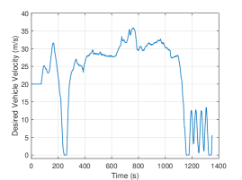
Figure 1: The desired velocity profile for the platoon.

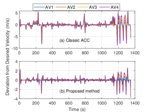
Figure 2: Velocity deviations: Case 1.

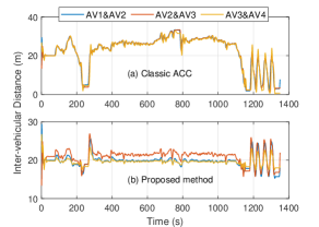
Figure 3: Inter-vehicular distances: Case 1.

When designing controllers for all the 4 AVs using a single SDP problem (III), solving the SDP needs 145.4 s. By splitting the platoon into two sub-platoons (one contains AV1&AV2 and another contains AV3&AV4), the control design is divided into two SDP problems each for a sub-platoon. Solving the two SDPs requires 17.1 s and 11.4 s, respectively. This confirms the discussions in Remark III.1.

The controllers solved from two sub-platoon SDP problems are implemented. Fig. 2 shows that the proposed method enables the platoon to follow the desired velocity profile closely and has smaller velocity deviations than the classic ACC. Consequently, the proposed method keeps the inter-vehicular distances close to the desired value $h^{*}=20~{}\mathrm{m}$, as seen from Fig. 3.

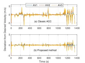
Figure 4: Velocity deviations: Case 2.

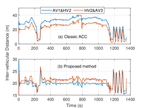
Figure 5: Inter-vehicular distances: Case 2.

Case 2: Mixed vehicle platoon. A mixed platoon with 3 vehicles, 2 AVs at the front and rear and an HV in the middle, is simulated. The AVs parameters are the same as Case 1. The HV parameters are $h_{s}=5~{}\mathrm{m}$, $h_{g}=50~{}\mathrm{m}$, $v_{\max}=40~{}\mathrm{m/s}$, $\tau=0.7~{}\mathrm{s}$, $\alpha=0.2$, and $\beta=0.4$. The initial vehicle state $(p_{i},v_{i},a_{i})$, $i\in[1,3]$, are randomly set as: $(45,20,0)$, $(20,15,0)$ and $(0,20,0)$, respectively. The sampling time, number of data samples, desired inter-vehicular distance and velocity profile are the same as Case 1.

Solving the SDP requires 18.2 s. As shown in Fig. 4 and Fig. 5, compared to the classic ACC, the proposed method enables the platoon to follow the velocity profile more closely whilst having inter-vehicular distances that are closer to the desired value $h^{*}=20~{}\mathrm{m}$.

VI Conclusion

A data-driven CACC is proposed for vehicle platoons with consideration of the unknown nonlinear vehicle dynamics. The controller design is formulated as an SDP problem that can be efficiently solved using off-the-shelf solvers. The proposed data-driven control design is applicable to platoons of pure AVs and also platoons of mixed AVs and HVs. The simulation results demonstrate that the proposed method is more effective than the classic ACC in establishing a stable vehicle platoons under a representative aggressive velocity reference. Future work will focus on incorporating input and safety constraints into the proposed data-driven control design to provide formal guarantee on platoon safety.

References

• [1] B. Van Arem, C. J. Van Driel, and R. Visser, “The impact of cooperative adaptive cruise control on traffic-flow characteristics,” IEEE Trans. Intell. Transp. Syst., vol. 7, no. 4, pp. 429–436, 2006.
• [2] J. Ploeg et al., “Design and experimental evaluation of cooperative adaptive cruise control,” in Proc. ITSC.   IEEE, 2011, pp. 260–265.
• [3] J. Yang et al., “Eco-driving of general mixed platoons with CAVs and HDVs,” IEEE trans. intell. veh., DOI: 10.1109/TIV.2022.3224679, 2022.
• [4] L. Xiao and F. Gao, “A comprehensive review of the development of adaptive cruise control systems,” Veh. Syst. Dyn., vol. 48, no. 10, pp. 1167–1192, 2010.
• [5] S. E. Shladover, D. Su, and X.-Y. Lu, “Impacts of cooperative adaptive cruise control on freeway traffic flow,” Transp. Res. Rec., vol. 2324, no. 1, pp. 63–70, 2012.
• [6] G. Gunter et al., “Are commercially implemented adaptive cruise control systems string stable?” IEEE Trans. Intell. Transp. Syst., vol. 22, no. 11, pp. 6992–7003, 2021.
• [7] J. Guanetti, Y. Kim, and F. Borrelli, “Control of connected and automated vehicles: State of the art and future challenges,” Annu. Rev. Control, vol. 45, pp. 18–40, 2018.
• [8] J. Lan and D. Zhao, “Min-max model predictive vehicle platooning with communication delay,” IEEE Trans. Veh. Technol., vol. 69, no. 11, pp. 12 570–12 584, 2020.
• [9] C. Chen et al., “Mixed platoon control of automated and human-driven vehicles at a signalized intersection: dynamical analysis and optimal control,” arXiv preprint, arXiv:2010.16105, 2020.
• [10] S. Feng et al., “Robust platoon control in mixed traffic flow based on tube model predictive control,” arXiv preprint, arXiv:1910.07477, 2019.
• [11] D. Hajdu, I. G. Jin, T. Insperger, and G. Orosz, “Robust design of connected cruise control among human-driven vehicles,” IEEE Trans. Intell. Transp. Syst., vol. 21, no. 2, pp. 749–761, 2019.
• [12] J. Lan, D. Zhao, and D. Tian, “Data-driven robust predictive control for mixed vehicle platoons using noisy measurement,” IEEE Trans. Intell. Transp. Syst., DOI: 10.1109/TITS.2021.3128406, 2021.
• [13] J. Shen, E. K. H. Kammara, and L. Du, “Nonconvex, fully distributed optimization based CAV platooning control under nonlinear vehicle dynamics,” IEEE Trans. Intell. Transp. Syst., DOI: 10.1109/TITS.2022.3175668, 2022.
• [14] A. Ghasemi, R. Kazemi, and S. Azadi, “Stable decentralized control of a platoon of vehicles with heterogeneous information feedback,” IEEE Trans. Veh. Technol., vol. 62, no. 9, pp. 4299–4308, 2013.
• [15] J. Hu et al., “Cooperative control of heterogeneous connected vehicle platoons: An adaptive leader-following approach,” IEEE Robot. Autom. Lett., vol. 5, no. 2, pp. 977–984, 2020.
• [16] W. Gao, Z.-P. Jiang, and K. Ozbay, “Data-driven adaptive optimal control of connected vehicles,” IEEE Trans. Intell. Transp. Syst., vol. 18, no. 5, pp. 1122–1133, 2016.
• [17] M. Huang, W. Gao, and Z.-P. Jiang, “Connected cruise control with delayed feedback and disturbance: An adaptive dynamic programming approach,” Int. J. Adapt. Control Signal Process., vol. 33, no. 2, pp. 356–370, 2019.
• [18] M. Huang, Z. P. Jiang, and K. Ozbay, “Learning-based adaptive optimal control for connected vehicles in mixed traffic: Robustness to driver reaction time,” IEEE Trans. Cybern., vol. 52, no. 6, pp. 5267–5277, 2020.
• [19] J. Wang, Y. Zheng, K. Li, and Q. Xu, “DeeP-LCC: Data-enabled predictive leading cruise control in mixed traffic flow,” arXiv preprint arXiv:2203.10639, 2022.
• [20] T. Chu and U. Kalabić, “Model-based deep reinforcement learning for CACC in mixed-autonomy vehicle platoon,” in Proc. IEEE Conf. Decis. Control.   IEEE, 2019, pp. 4079–4084.
• [21] Y. Zhu, J. Wu, and H. Su, “V2V-based cooperative control of uncertain, disturbed and constrained nonlinear CAVs platoon,” IEEE Trans. Intell. Transp. Syst., DOI: 10.1109/TITS.2020.3026877, 2020.
• [22] W. Gao and Z.-P. Jiang, “Nonlinear and adaptive suboptimal control of connected vehicles: A global adaptive dynamic programming approach,” J. Intell. Robot. Syst., vol. 85, no. 3, pp. 597–611, 2017.
• [23] R. Strässer, J. Berberich, and F. Allgöwer, “Data-driven control of nonlinear systems: Beyond polynomial dynamics,” in Proc. CDC.   IEEE, 2021, pp. 4344–4351.
• [24] C. De Persis, M. Rotulo, and P. Tesi, “Learning controllers from data via approximate nonlinearity cancellation,” IEEE Trans. Automat. Contr., DOI: 10.1109/TAC.2023.3234889, 2023.
• [25] S. E. Li et al., “Dynamical modeling and distributed control of connected and automated vehicles: Challenges and opportunities,” IEEE Intell. Transp. Syst. Mag., vol. 9, no. 3, pp. 46–58, 2017.
• [26] C. Scherer and S. Weiland, “Linear matrix inequalities in control,” Lecture Notes, Dutch Institute for Systems and Control, Delft, The Netherlands, vol. 3, no. 2, 2000.
• [27] J. Löfberg, “YALMIP: A toolbox for modeling and optimization in MATLAB,” in Proc. CACSD, vol. 3, 2004.
• [28] Mosek ApS, “The MOSEK optimization software.” [Online]. Available: https://www.mosek.com