Low NH₃/H₂O ratio in comet C/2020 F3 (NEOWISE) at $0.7$ au from the Sun

Abstract

Context. A lower-than-solar elemental nitrogen content has been demonstrated for several comets, including 1P/Halley and 67P/Churyumov-Gerasimenko (67P/C-G) with independent in situ measurements of volatile and refractory budgets. The recently discovered semi-refractory ammonium salts in 67P/C-G are thought to be the missing nitrogen reservoir in comets.

Aims. The thermal desorption of ammonium salts from cometary dust particles leads to their decomposition into ammonia (NH₃) and a corresponding acid. The NH₃/H₂O ratio is expected to increase with decreasing heliocentric distance with evidence for this in near-infrared observations. NH₃ has been claimed to be more extended than expected for a nuclear source. Here, the aim is to constrain the NH₃/H₂O ratio in comet C/2020 F3 (NEOWISE) during its July 2020 passage.

Methods. OH emission from comet C/2020 F3 (NEOWISE) was monitored for 2 months with the Nançay Radio Telescope (NRT) and observed from the Green Bank Telescope (GBT) on 24 July and 11 August 2020. Contemporaneously with the 24 July 2020 OH observations, the NH₃ hyperfine lines were targeted with GBT. From the data, the OH and NH₃ production rates were derived directly, and the H₂O production rate was derived indirectly from the OH.

Results. The concurrent GBT and NRT observations allowed the OH quenching radius to be determined at $\left(5.96\pm 0.10\right)\times 10^{4}$ km on 24 July 2020, which is important for accurately deriving $Q(\text{OH})$. C/2020 F3 (NEOWISE) was a highly active comet with $Q(\text{H}_{2}\text{O})\approx 2\times 10^{30}$ molec s^-1 one day before perihelion. The $3\sigma$ upper limit for $Q_{\text{NH}_{3}}/Q_{\text{H}_{2}\text{O}}$ is $<0.29\%$ at $0.7$ au from the Sun.

Conclusions. The obtained NH₃/H₂O ratio is a factor of a few lower than measurements for other comets at such heliocentric distances. The abundance of NH₃ may vary strongly with time depending on the amount of water-poor dust in the coma. Lifted dust can be heated, fragmented, and super-heated; whereby, ammonium salts, if present, can rapidly thermally disintegrate and modify the $\text{NH}_{3}/\text{H}_{2}\text{O}$ ratio.

1 Introduction

Comets are ice-rich, kilometer-sized bodies composed of volatiles, refractories, and semi-refractory compounds. The key characteristic of these minor bodies of our Solar System is their outgassing activity, especially upon their approach toward the Sun. During the approach, the volatile ices in a cometary nucleus are released as gases into a tenuous coma and dust particles are lifted off of the surface through several mechanisms (Jewitt & Hsieh, 2022). Based on their physical properties, it remains unclear if such bodies formed in a protoplanetary disk through hierarchical agglomeration of cometesimals or through pebble accretion (Weissman et al., 2020; Blum et al., 2022). The chemical composition of volatiles does support partial inheritance of ices from the earliest stages of star formation to cometary nuclei (Bockelée-Morvan et al., 2000; Drozdovskaya et al., 2019; Altwegg et al., 2019).

The dominant volatile constituent of comets is water (H₂O; Mumma & Charnley 2011). A typical, although not only, method for remote sensing of cometary water is through observations of OH (Schloerb & Gérard, 1985), which is a primary product of H₂O photodissociation in the coma. OH lines are available in the UV (Feldman et al., 2004; Bodewits et al., 2022), radio (Crovisier et al., 2002a, b), and infrared (IR; Bonev et al. 2006; Bonev & Mumma 2006) regimes. The production rate of H₂O is a fundamental parameter of a comet that must be constrained for each comet individually and over the longest-possible period of time in order to get a handle on the individual time-dependent cometary activity. In turn, this facilitates comparisons of chemical compositions from comet to comet relative to the dominant volatile species, H₂O.

The nitrogen budget of comets has been a long-standing mystery, because even summing all the volatile N measured in the coma with the refractory N measured in the dust leaves a deficiency in N relative to the solar N/C ratio (Geiss, 1988; Rubin et al., 2015; Biver et al., 2022b). The recent discovery of ammonium salts (NH${}_{4}^{+}$X^-) on the dust grains of comet 67P/Churyumov-Gerasimenko (hereafter, 67P/C-G) is thought to have uncovered the missing reservoir of nitrogen in comets (Poch et al., 2020; Altwegg et al., 2020). Their presence was already hypothesized on the basis of data for comet 1P/Halley (Wyckoff et al., 1991) and the salt NH${}^{+}_{4}$CN^- was suggested to be the precursor for NH₃ and HCN release in more recent comets (Mumma et al., 2017, 2018, 2019). Ammonium salts are considered to be semi-volatile with sublimation temperatures in the $160-230$ K range (Bossa et al., 2008; Danger et al., 2011). In the laboratory, it was demonstrated that ammonia (NH₃) is a key product of thermal desorption of ammonium salts that decompose during this process (Hänni et al., 2019; Kruczkiewicz et al., 2021). Consequently, it is expected that as the comet’s heliocentric distance decreases, its ammonium salts desorb and decompose, which in turns leads to an increasing NH₃/H₂O ratio. This trend was demonstrated on the basis of high-resolution IR spectroscopic observations of $30$ comets (fig. $7$b of Dello Russo et al. 2016). To an extent, this is also seen in the NH₃/H₂O ratio measured with the Rosetta Orbiter Spectrometer for Ion and Neutral Analysis (ROSINA; Balsiger et al. 2007) instrument aboard the ESA Rosetta spacecraft during its 2-yr long monitoring of 67P/C-G, although there is quite a bit of scatter in the ratio that is uncorrelated with the latitude and season (fig. $1$a of Altwegg et al. 2020).

Ammonium salts have also been detected on the surface of the dwarf planet Ceres with the Dawn mission (de Sanctis et al., 2015; De Sanctis et al., 2019), but they have not been detected in interstellar ices thus far (Boogert et al., 2015). However, their presence has long been hypothesized (Lewis & Prinn, 1980) and expected based on a suite of laboratory experiments involving the UV irradiation or electron bombardment of NH₃-containing ices (Grim et al., 1989; Bernstein et al., 1995; Muñoz Caro & Schutte, 2003; Gerakines et al., 2004; van Broekhuizen et al., 2004; Bertin et al., 2009; Vinogradoff et al., 2011). It has also been demonstrated in the laboratory that acid-base grain-surface reactions between NH₃ and HNCO, NH₃ and HCN, and NH₃ and HCOOH may form the ammonium cyanate (NH${}^{+}_{4}$OCN^-), ammonium formate (NH${}^{+}_{4}$HCOO^-), and ammonium cyanide (NH${}^{+}_{4}$CN^-) salts, respectively, even at prestellar core temperatures of $\sim 10$ K without energetic processing and increase in efficiency with elevated temperatures (Schutte et al., 1999; Raunier et al., 2003, 2004; Gálvez et al., 2010; Mispelaer et al., 2012; Noble et al., 2013; Bergner et al., 2016). At a warmer temperature of $80$ K, NH₃ and CO₂ have also been experimentally shown to react to produce ammonium carbamate (NH${}^{+}_{4}$H₂NCOO^-; Bossa et al. 2008).

Detections of the NH₃ hyperfine inversion lines, which arise from the oscillation of the nitrogen atom through the plane formed by the three hydrogens, have been challenging to secure on a consistent basis in comets. A possible detection of the $J_{K}=3_{3}-3_{3}$ inversion line at $23.870$ GHz was made in comet C/1983 H1 (IRAS-Araki-Alcock) with the Effelsberg 100-m telescope (Altenhoff et al., 1983). A sensitive search for the same line with the same instrument in comets 1P/Halley and 21P/Giacobini–Zinner was negative (Bird et al., 1987), which was also the case for the earlier comet C/1973 E1 (Kohoutek) (Churchwell et al., 1976). A confirmed detection of the $J_{K}=1_{1}-1_{1}$ and $3_{3}-3_{3}$ inversion lines with high signal-to-noise ratios was obtained in C/1996 B2 (Hyakutake) with the 43-m telescope of the National Radio Astronomy Observatory (NRAO) in Green Bank (Palmer et al., 1996). In comet C/1995 O1 (Hale-Bopp), all inversion transitions from $J_{K}=1_{1}-1_{1}$ to $5_{5}-5_{5}$ were detected with the Effelsberg 100-m telescope (Bird et al., 1997). Some of these were also observed with the NRAO 43-m telescope (Butler et al., 2002) and the 45-m telescope of the Nobeyama Radio Observatory (Hirota et al., 1999). Despite a sensitive search at the Effelsberg 100-m telescope, NH₃ was not detected in comets C/2001 A2 (LINEAR) , C/2001 Q4 (NEAT), and C/2002 T7 (LINEAR), and only marginally detected in comet 153P/Ikeya-Zhang (Bird et al., 2002; Hatchell et al., 2005a). Subsequent rotational lines, which are stronger, lie at submillimeter wavelengths. NH₃ was detected in several comets (Table 5) using the Odin and Herschel satellites through its $J_{K}=1_{0}-0_{0}$ transition at $572$ GHz that is only accessible from space (Biver et al., 2007, 2012). This transition was also monitored in comet 67P/C-G with the Microwave Instrument for the Rosetta Orbiter (MIRO) instrument aboard Rosetta (Gulkis et al., 2007; Biver et al., 2019). At shorter IR wavelengths, NH₃ has been observed in many comets (Table 5) through its vibrational lines near $3\leavevmode\nobreak\ \mu$m, although its unblended lines are sparse and weak in comparison to other species typically observed in the near-IR (Dello Russo et al. 2016, 2022; Bonev et al. 2021 and the many references therein).

In this paper, we present radio observations of comet C/2020 F3 (NEOWISE), hereafter F3 for simplicity, taken at the Nançay Radio Telescope (NRT) and the Green Bank Telescope (GBT) that targeted OH and NH₃ lines (Table 1). The long-period comet F3 originating from the Oort Cloud was a bright naked-eye object in the sky that underwent perihelion on 3 July 2020 and perigee on 22-23 July 2020. A more detailed description of the comet is given in Section 2.1. The OH emission from the comet was monitored nearly continuously for 2 months at the NRT pre- and post-perihelion. GBT observations targeted contemporaneously OH and NH₃ lines post-perihelion on 24 July 2020. Additional OH data were collected at the GBT on 11 August 2020. The GBT observational strategy and data reduction are presented in Section 2.2. The NRT observations are described in Section 2.3. The methods behind the determination of the OH production rate are described in Section 3.1.1. The analysis of OH line profiles in the context of outflow velocities is in Section 3.1.2. GBT and NRT OH observations taken on the same date, a mere $2$ hours apart, are used to constrain the OH quenching radius in Section 3.1.3 based directly on observational data, which is critical for an accurate determination of the OH production rate. The GBT OH observations of 11 August 2020 are analyzed in the context of the Greenstein effect in Section 3.1.4. The OH and H₂O production rates are finally computed in Section 3.1.5. GBT NH₃ observations are analyzed in Section 3.2 and discussed in the context of the NH₃/H₂O ratio as a function of heliocentric distance in Section 4. The conclusions of the work can be found in Section 5.

Table 1: Targeted lines.

Line	Frequency
	(MHz)
OH ${}^{2}\Pi_{3/2}\leavevmode\nobreak\ J=3/2\leavevmode\nobreak\ F=1-2$	$1\leavevmode\nobreak\ 612.2309$
OH ${}^{2}\Pi_{3/2}\leavevmode\nobreak\ J=3/2\leavevmode\nobreak\ F=1-1$	$1\leavevmode\nobreak\ 665.4018$
OH ${}^{2}\Pi_{3/2}\leavevmode\nobreak\ J=3/2\leavevmode\nobreak\ F=2-2$	$1\leavevmode\nobreak\ 667.3590$
OH ${}^{2}\Pi_{3/2}\leavevmode\nobreak\ J=3/2\leavevmode\nobreak\ F=2-1$	$1\leavevmode\nobreak\ 720.5299$
NH3 $J_{K}=1_{1}-1_{1}$	$23\leavevmode\nobreak\ 694.4955$
NH3 $J_{K}=2_{2}-2_{2}$	$23\leavevmode\nobreak\ 722.6333$
NH3 $J_{K}=3_{3}-3_{3}$	$23\leavevmode\nobreak\ 870.1292$
NH3 $J_{K}=4_{4}-4_{4}$	$24\leavevmode\nobreak\ 139.4163$
NH3 $J_{K}=5_{5}-5_{5}$	$24\leavevmode\nobreak\ 532.9887$

2 Observations of comet C/2020 F3 (NEOWISE)

2.1 Comet C/2020 F3 (NEOWISE)

Comet F3 is considered to be the brightest comet in the northern hemisphere since comet C/1995 O1 (Hale-Bopp) in 1997 (Fig. 1). It was a bright naked-eye target in midsummer of 2020 and termed by some as the “Great Comet of 2020”. Comet F3 showed a huge ($\sim 10^{5}$ km), curving, banded dust tail and a much fainter, straight, blue ion tail ($\sim 10^{6}$ km). It was viewed from the International Space Station (ISS) and photographed by countless members of the public. F3 is a long-period comet originating from the Oort Cloud with an orbital period of $\sim 4\leavevmode\nobreak\ 500$ yr and a near-parabolic (eccentricity of $0.999$) trajectory. It was discovered on March 27th, 2020 by the Near Earth Object Wide-field Infrared Survey Explorer (NEOWISE) mission of the Wide-field Infrared Survey Explorer spacecraft (Mainzer et al. 2011). Perihelion took place on July 3rd, 2020 at $0.295$ au from the Sun and perigee occurred in the night from July 22nd to 23rd, 2020 at $0.692$ au from the Earth. Its nucleus was estimated to be approximately $5$ km in diameter (Bauer et al., 2020) with a rotation period of $7.8\pm 0.2$ h (Manzini et al., 2021). Sudden short-lived outbursts have not been reported for comet F3 and none were observed during the extended (from May to September 2020) monitoring campaign of the comet by the Solar Wind ANisotropies (SWAN) camera on the Solar and Heliospheric Observatory (SOHO) spacecraft (Combi et al., 2021). However, strong jet activity is seen in the HST images taken on 8 August 2020 (Program ID: 16418, P.I.: Qicheng Zhang). There were also no signs of disintegration pre-perihelion based on NASA/ESA’s Solar and Heliospheric Observatory (SOHO) LASCO C3 coronagraph observations (Knight & Battams, 2020).

Comet F3 was observed by several facilities in the optical regime. Observations with the High Accuracy Radial velocity Planet Searcher for the Northern hemisphere (HARPS-N) echelle spectrograph on the 360-cm Telescopio Nazionale Galileo (TNG) with a high resolving power ($R$) of $115\leavevmode\nobreak\ 000$ revealed detections of C₂, C₃, CN, CH, NH₂, Na, and [O I] (taken on 26 July and 5 August 2020; Cambianica et al. 2021). Lines of C₂, NH₂, Na, and [O I] were also detected with low resolution, $R=7\leavevmode\nobreak\ 400-9\leavevmode\nobreak\ 300$, observations made with the Échelle spectrograph FLECHAS at the 90-cm telescope of the University Observatory Jena taken on 21, 23, 29, 30, and 31 July 2020 (Bischoff & Mugrauer 2021; Na was detected only on the first two dates). Lines of C₂, C₃, CN, CH, NH₂, Na, and [O I] were also detected with the Tull Coudé Spectrograph at $R=60\leavevmode\nobreak\ 000$ on the 2.7-m Harlan J. Smith Telescope at McDonald Observatory on 24 July and 11 August 2020 (Cochran et al., 2020). Lines of C₂, C₃, CN, NH₂, Na, [O I], K, and H₂O⁺ were also detected with ultra-high resolution spectroscopy at $R=140\leavevmode\nobreak\ 000$ with the EXtreme PREcision Spectrograph (EXPRES) on the 4.3-m Lowell Discovery Telescope on 15 and 16 July 2020 (Ye et al., 2020). Further chemical characterization of comet F3 was executed in the IR. In the $1.1-5.3$ $\mu$m range, data were taken with the long-slit near-IR high-resolution ($R=35\leavevmode\nobreak\ 000-70\leavevmode\nobreak\ 000$) immersion echelle spectrograph iSHELL at the NASA/IRTF facility. The $0.95-5.5$ $\mu$m range was observed with NIRSPEC 2.0 ($R=25\leavevmode\nobreak\ 000-37\leavevmode\nobreak\ 500$) at the Keck Observatory. These near-IR observations of Faggi et al. (2021) led to the detection of $9$ primary volatiles (H₂O, HCN, NH₃, CO, C₂H₂, C₂H₆, CH₄, CH₃OH, and H₂CO) and $3$ product species (CN, NH₂, OH^∗) on several dates in July and August 2020. In the radio, comet F3 was observed with the Institut de Radio Astronomie Millimétrique (IRAM) 30-m and the NOrthern Extended Millimeter Array (NOEMA) telescopes on several dates in July and August with secured detections of HCN, HNC, CH₃OH, CS, H₂CO, CH₃CN, H₂S, and CO (Biver et al., 2022a).

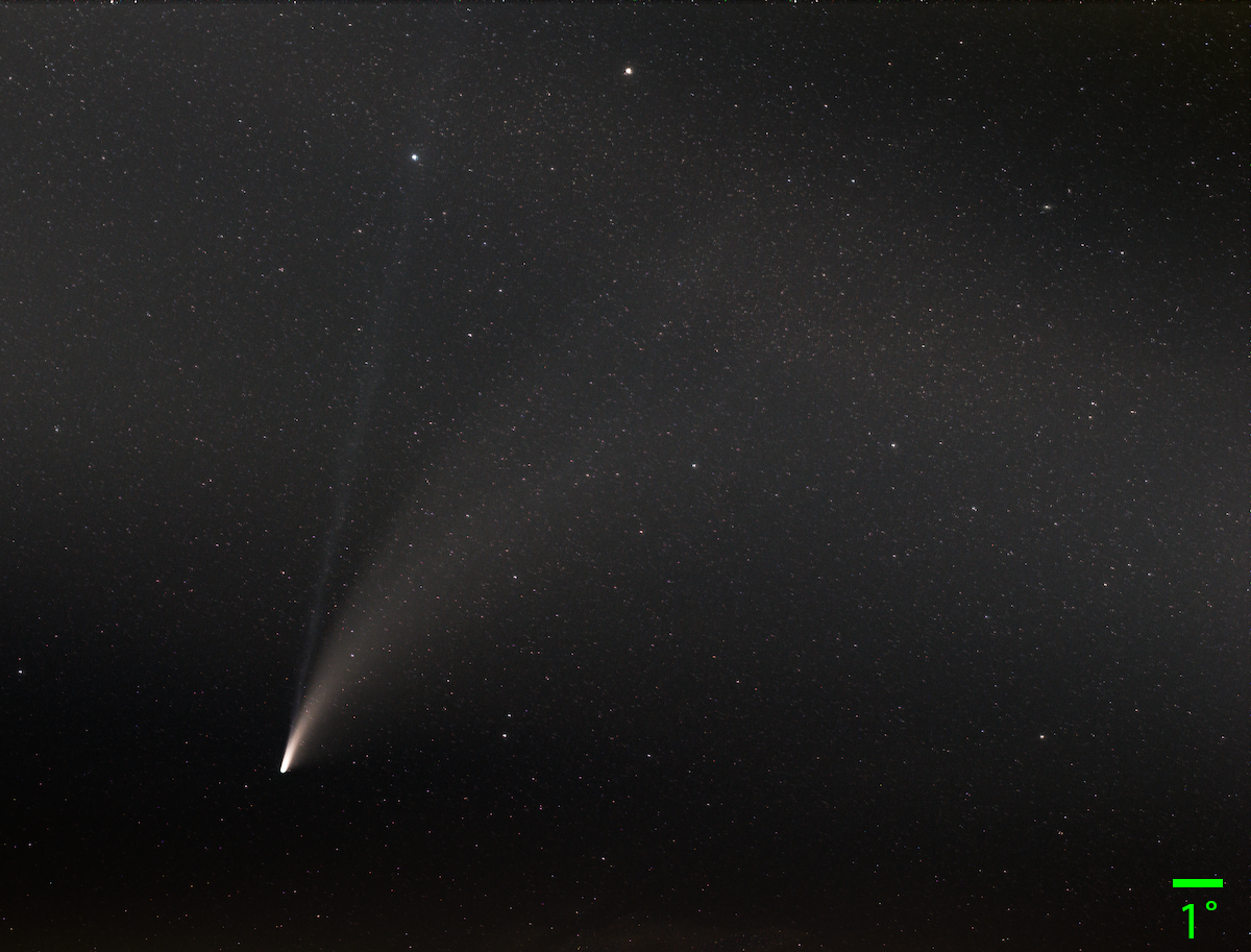
Figure 1: Comet C/2020 F3 (NEOWISE) as seen from the Blue Ridge Mountains outside of White Hall, Virginia on 20 July 2020. The image is an aligned and stacked average of five, 5-minute exposures taken using a Nikon D750 DLSR camera with a $50$ mm $f/1.8$ lens held on an equatorial tracking mount (B. A. McGuire). The image is approximately $29.3^{\circ}\times 22.3^{\circ}$ in total. The $1^{\circ}$ scale is indicated in the lower right corner, which corresponds to $3\times 10^{4}$ km at the geocentric distance of the comet on this date. A finder chart for this image is available at https://nova.astrometry.net/user_images/7997658# (Lang et al., 2010).

2.2 Green Bank Telescope observations

Comet F3 was observed with the Robert C. Byrd 100-m GBT in Green Bank, West Virginia under the project code GBT20A-587. The Director’s Discretionary Time (DDT) proposal was awarded a total amount of $12$ h, which was to be executed in two $6$ h sessions with a separation of at least $3$ days to probe dependencies with heliocentric distance. It was planned for each session to begin with $1$ h of OH observations, followed immediately by $5$ h of NH₃ observations (including $5$ and $40$ min of overheads, respectively). The targeted lines are tabulated in Table 1. Due to an unfortunate overlap of the comet’s perihelion on 3 July 2020 with scheduled maintenance, both sessions were observed post-perihelion.

Table 2: GBT and NRT half-power beam widths (HPBWs) and efficiencies.

Facility	Frequency	$\theta_{\text{HPBW}}$	$\eta_{\text{A}}$	$\eta_{\text{mB}}$
	(GHz)	($\arcmin$)
GBT	$1.67$	$7.55\pm 0.083$	$0.72^{a}$	$0.95^{b}$
GBT	$23.8$	$0.53\pm 0.005$	$0.68^{a}$	$0.91^{b}$
NRT	$1.67$	$3.5\times 19$	$0.46$	$0.65^{c}$

^a Aperture efficiency ($\eta_{\text{A}}$) from the GBO Proposer’s Guide for the GBT of 3 January 2023.
^b Main beam efficiency deduced from $\eta_{\text{mB}}=\eta_{\text{A}}S_{\text{tel}}\Omega/\lambda^{2}$, where $S_{\text{tel}}$ is the GBT surface telescope area ($7\leavevmode\nobreak\ 854$ m²), $\lambda$ is the wavelength, and $\Omega$ is the solid angle of the Gaussian beam defined by the HPBW in radians, which is given by $\Omega=\pi\theta_{\text{HPBW}}^{2}/4\ln 2$.
^c Assuming a conversion factor of $0.85$ K Jy^-1 and an effective area of $7\leavevmode\nobreak\ 000$ m².

2.2.1 Day 1 and 2 OH observations

OH observations were carried out with the L-band receiver coupled with the VErsatile GBT Astronomical Spectrometer (VEGAS) backend (Roshi et al., 2011). For the first session, on day 1 (24.71 July 2020), mode $8$ was used with a $100$ MHz bandwidth, $65\leavevmode\nobreak\ 536$ channels, and a spectral resolution of $1.5$ kHz ($0.3$ km s^-1 at $1\leavevmode\nobreak\ 666.0$ MHz). These were single beam, dual polarization observations carried out with in-band frequency switching with a throw of $25$ MHz (centered on the rest frequency of $1\leavevmode\nobreak\ 666.0$ MHz). For the second session, on day 2 (11.88 August 2020), the signal was routed to four banks of VEGAS in four different modes: mode $8$ (same as day 1), mode $9$ ($100$ MHz bandwidth, $131\leavevmode\nobreak\ 072$ channels, $0.8$ kHz or $0.14$ km s^-1 spectral resolution), mode $11$ ($23.44$ MHz bandwidth, $65\leavevmode\nobreak\ 536$ channels, $0.4$ kHz or $0.07$ km s^-1 spectral resolution), and mode $12$ ($23.44$ MHz bandwidth, $131\leavevmode\nobreak\ 072$ channels, $0.2$ kHz or $0.04$ km s^-1 spectral resolution). At the start of observing on both days, pointing and focus were performed using the Digital Continuum Receiver (DCR) backend toward the calibrator source 1011+4628 across a $80$ MHz bandwidth. The half-power beam width (HPBW) of the GBT at $1.67$ GHz is $(7.55\pm 0.083)\arcmin$ (according to equation $2$ of the Green Bank Observatory (GBO) Proposer’s Guide for the GBT of 3 January 2023).

Day 1 OH observations were executed starting 24.71 July 2020. The total integration time on-source was $46$ min ($23$ scans, $2$ min each). Day 2 observations were taken starting 11.88 August 2020. Due to the separation between the two sessions being $17$ days (much longer than the initially envisioned separation of not much more than $3$ days) and the non-detection of NH₃ at the more favorable smaller heliocentric distance of Day 1 (Section 2.2.2), the remaining allocated time was dedicated solely to OH observations. However, this time, the observations were performed toward three different locations: on-comet, an offset toward the Sun, and an offset away from the Sun. The integration time was $1$ h $26$ min ($43$ scans, $2$ min each) on-comet, $1$ h $38$ min ($49$ scans, $2$ min each) toward-offset, and $1$ h $58$ min ($59$ scans, $2$ min each) away-offset. Total on-source time was $5$ h $2$ min. It was envisioned to probe one-beam offsets from the on-comet position along the Sun-comet trajectory to accurately quantify the quenching radius of OH (analogously to the methods of Colom et al. (1999) for comet C/1995 O1 (Hale-Bopp)). However, due to an error in offset coordinates in the observing script, the probed positions were $\sim 8$ beams away in RA to the northeast (and $<1/5$ of a beam away in Dec to the southwest). Specifically, the toward-offset was RA, Dec (J2000) of -7m30s, +1$\arcmin$20$\arcsec$ and the away-offset was RA, Dec (J2000) of +7m30s, -1$\arcmin$20$\arcsec$.

The OH $1\leavevmode\nobreak\ 665$ and $1\leavevmode\nobreak\ 667$ MHz spectra obtained on Day 1 (24.71 July 2020) at the GBT are shown in Fig. 2. The OH $1\leavevmode\nobreak\ 667$ MHz spectrum obtained on Day 2 (11.88 August 2020) at the GBT is shown in Fig. 3. L-band Day 1 data have been checked for the presence of the ¹⁸OH line at $1\leavevmode\nobreak\ 639.5$ MHz (the strongest of three ¹⁸OH lines in range), but it was not detected. The observed frequency range also covered one line of ¹⁷OH, but based on neither the isotopic ratio of ${}^{18}\text{O}/^{17}\text{O}=3.6$ in the local interstellar medium (ISM; Wilson 1999) nor the measured ${}^{18}\text{O}/^{17}\text{O}=5.3\pm 0.4$ in water of comet 67P/C-G (Schroeder et al., 2019; Müller et al., 2022), it is not expected to be detected if ¹⁸OH is not. The main beam efficiencies ($\eta_{\text{mB}}$) given in Table 2 were used to convert the line areas into the main beam brightness temperature scale through $T_{\text{mB}}=T_{\text{A}}^{*}/\eta_{\text{mB}}$. Table 3 gives line areas in $T_{\text{A}}^{*}$ scale for the OH lines observed at the GBT. The ratio of the line areas of the $1\leavevmode\nobreak\ 667$ and $1\leavevmode\nobreak\ 665$ MHz OH lines observed on 24 July 2020 is $1.93\pm 0.07$, which is consistent, within $2\sigma$, with the statistical ratio of $1.8$.

2.2.2 Day 1 NH₃ observations

NH₃ observations were carried out on Day 1 (starting 24.81 July 2020). The $7$-pixel K-band Focal Plane Array (KFPA) receiver (Masters et al., 2011) was employed with the VEGAS backend. The total integration time on-source was $3$ h $34$ min ($107$ scans, $2$ min each). Mode $24$ was used with a $23.44$ MHz bandwidth, $65\leavevmode\nobreak\ 536$ channels, and a spectral resolution of $0.4$ kHz ($0.005$ km s^-1 at $23.8$ GHz). All seven beams of the KFPA were used and routed to six banks of VEGAS (centered on rest frequencies of $23\leavevmode\nobreak\ 694.50$, $23\leavevmode\nobreak\ 722.63$, $23\leavevmode\nobreak\ 870.13$, $24\leavevmode\nobreak\ 139.42$, $24\leavevmode\nobreak\ 532.99$, $23\leavevmode\nobreak\ 963.9$ MHz). These were dual polarization observations carried out with in-band frequency switching with a throw of $5$ MHz. At the start of observing, pointing and focus were performed using a single spectral window (still with the VEGAS backend) toward the calibrator source 1033+4116 across a $1\leavevmode\nobreak\ 500$ MHz bandwidth (centered on the rest frequency of $24\leavevmode\nobreak\ 010$ MHz). The HPBW of the GBT at $23.8$ GHz is $(0.53\pm 0.005)\arcmin$ (Table 2). The data from all seven beams were inspected for the presence of NH₃ lines individually; however, solely the centermost on-comet beam has been used for the derivation of the upper limits. Table 3 gives the upper limits in $T_{\text{A}}^{*}$ scale on the NH₃ lines observed at the GBT.

2.2.3 GBT data reduction

Initial data processing and calibration were performed using GBTIDL. Day 1 OH and NH₃ observations were visually inspected on a scan-by-scan basis. All scans were considered for the final data products with folding performed using the getfs routine. The final spectra are noise-weighted averages of all the scans and both polarizations for the case of L-band observations. For the KFPA data, only the right polarization has been considered given a known and reported issue with the left polarization at the time these observations were taken. Day 2 OH observations suffered from much more severe Radio Frequency Interference (RFI). Furthermore, a mishap occurred for modes $11$ and $12$, because the adopted $25$ MHz throw exceeded the bandwidth, resulting in there being no overlap between the sig and ref phases. All $151$ scans were visually inspected in the sig and ref phases (for modes $8$ and $9$; and only in the sig phase for modes $11$ and $12$) separately in both polarizations in small regions near the two OH lines. Scans with severe RFI or odd baselines (even if in just one polarization of either of the phases) were discarded. All scans in the ref phase of modes $8$ and $9$ exhibit an RFI close to $(1667.36-25.00)=1642.36$ MHz, which after folding results in an absorption artifact close to the $1\leavevmode\nobreak\ 667.36$ MHz OH line. Consequently, all data in the ref phase from all $4$ modes were discarded in the analysis of the $1\leavevmode\nobreak\ 667.36$ MHz OH line. As a result, calibration of the sig phase had to be done manually on the basis of a line- and RFI-free region, and the application of the noise diode in K factor. With this methodology, any remaining absorption feature must be a real signal rather than an artifact of folding. In the analysis of the $1\leavevmode\nobreak\ 665.40$ MHz OH line, both sig and ref phases were considered from modes $8$ and $9$ with folding using the getfs routine, but only the sig phase from modes $11$ and $12$ was considered with the manual calibration procedure. Finally, for every mode a noise-weighted average was produced. These spectra were then resampled to the coarsest spectral resolution of mode $8$ ($1.5$ kHz). The resampling has been performed with the Flux Conserving Resampler from the specutils Python package, which conserves the flux during the resampling process (Carnall, 2017). The final spectrum per OH line per position is a noise-weighted average of the four modes.

For the Day 1 OH data, baseline subtraction was performed (separately for each line) on a scan-by-scan basis with a first-order polynomial in a region centered on the rest-frequency of the specific OH line, which corresponds to $\pm 54$ km s^-1 ($\pm 300$ kHz or $\pm 200$ channels), while excluding the central $\pm 2$ km s^-1 ($\pm 11$ kHz or $\pm 8$ channels) range that includes the line. For the NH₃ data, baseline subtraction was performed (separately for each line) on a scan-by-scan basis with a first-order polynomial in a region centered on the rest-frequency of the specific NH₃ line, which corresponds to $\pm 8$ km s^-1 ($\pm 633$ kHz or $\pm 1766$ channels), while excluding the central $\pm 2$ km s^-1 ($\pm 158$ kHz or $\pm 442$ channels) range that includes the line. For the Day 2 OH data, baseline subtraction was performed on a scan-by-scan basis with a first-order polynomial in a $0.54-0.76$ (depending on the mode) and $0.2$ MHz wide region near the rest-frequencies of the $1\leavevmode\nobreak\ 665.40$ and $1\leavevmode\nobreak\ 667.36$ MHz OH lines, respectively. The baseline subtraction was performed solely on the sig phase for the cases when it was the only phase used for the final product (all modes for the $1\leavevmode\nobreak\ 667.36$ MHz line, and modes $11$ and $12$ for the $1\leavevmode\nobreak\ 665.40$ MHz line). The observed spectra were corrected by the comet’s velocity on a scan-by-scan basis based on computations (with a step size of $1$ min) from NASA/JPL Horizons On-Line Ephemeris System (EOP files eop.210205.p210429 and eop.210211.p210505).

The system temperature ($T_{\text{sys}}$) on Day 1 in the L-band was in the $16.76-19.41$ K range with a mean of $18.01$ K. $T_{\text{sys}}$ on Day 2 in the L-band was in the $11.14-25.79$, $8.77-27.91$, and $17.36-28.14$ K ranges with means of $20.37$, $20.21$, and $21.65$ K at the on-comet, toward-offset, and away-offset positions, respectively. $T_{\text{sys}}$ on Day 1 for the KFPA was in the $69.55-88.29$ K range with a mean of $76.43$ K (in the central beam of the KFPA), which was on the higher end of expectations. The anticipated RMS based on the GBT Sensitivity Calculator was estimated to be in the $2.7-5.4$ mK km s^-1 range for $T_{\text{sys}}\in\left[50-100\right]$ K in the proposal for the KFPA for a line width of $3$ km s^-1. However, the attained RMS of the observations came out to be $46-48$ mK channel^-1 (in the central beam of the KFPA), which corresponds to $5.6-5.9$ mK km s^-1 for a line width of $3$ km s^-1 (using $\text{RMS}(\text{mK\leavevmode\nobreak\ km\leavevmode\nobreak\ s}^{-1})=\sqrt{n}\times\text{RMS}(\text{mK\leavevmode\nobreak\ channel}^{-1})\times dv$, where $dv$ is the channel width and $n$ is the number of channels spanning the line). Other KFPA beams had comparable $T_{\text{sys}}$ and RMS values, except for the sixth beam, which was a factor of $1.7$ higher. The somewhat higher attained RMS in comparison to the anticipated RMS from the GBT Sensitivity Calculator stems from the actual on-source time being $46$ min shorter than planned and the $T_{\text{sys}}$ values being in the higher range of expectations. All spectra are in terms of the antenna temperature corrected for antenna and atmospheric losses, $T_{\text{A}}^{*}$ (Ulich & Haas, 1976). In the K-band, the calibration uncertainty is generally $\sim 30\%$ for the GBT (McGuire et al., 2020; Sita et al., 2022).

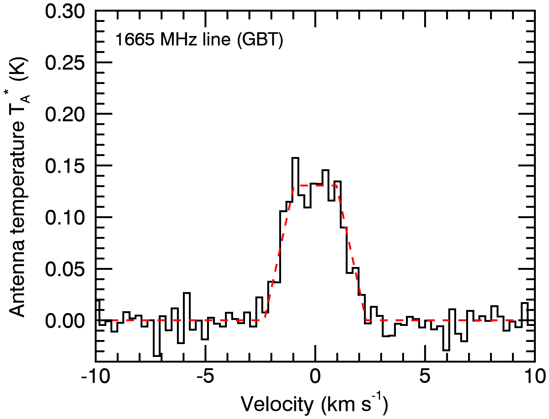
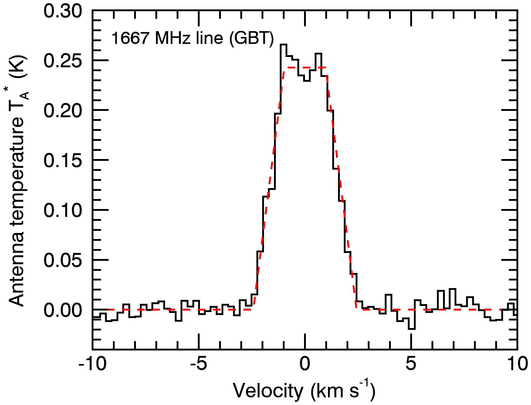
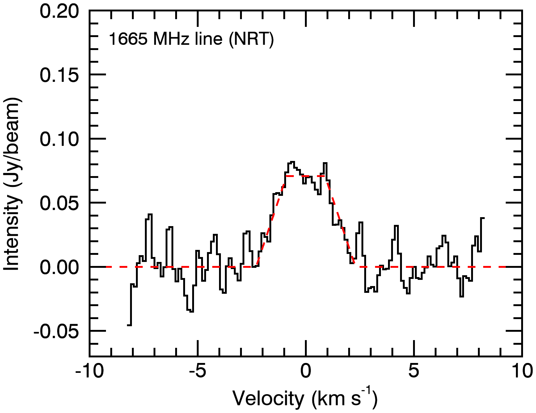
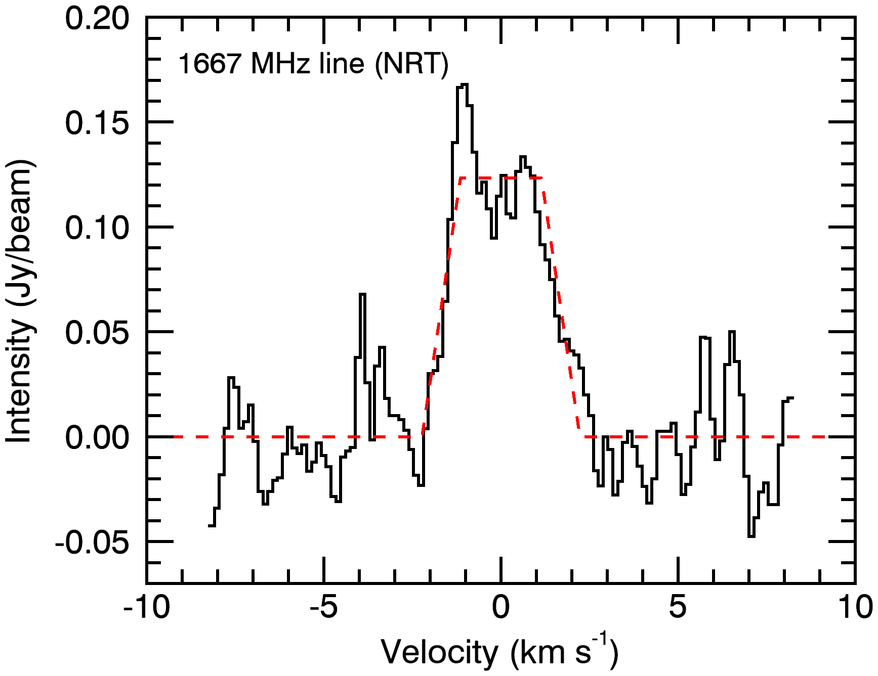
Figure 2: OH $1\leavevmode\nobreak\ 665$ (left) and $1\leavevmode\nobreak\ 667$ MHz (right) lines observed with the GBT (top) and the NRT (bottom) on 24 July 2020 in solid black lines. The red dashed curves show the fitted trapeziums to the spectra based on the methodology of Bockelée-Morvan et al. (1990). For GBT (NRT), the half lower bases of the trapeziums are $2.32\pm 0.07$ ($2.30\pm 0.14$) and $2.43\pm 0.03$ ($2.23\pm 0.11$) km s^-1 for the $1\leavevmode\nobreak\ 665$ and $1\leavevmode\nobreak\ 667$ MHz lines, respectively.

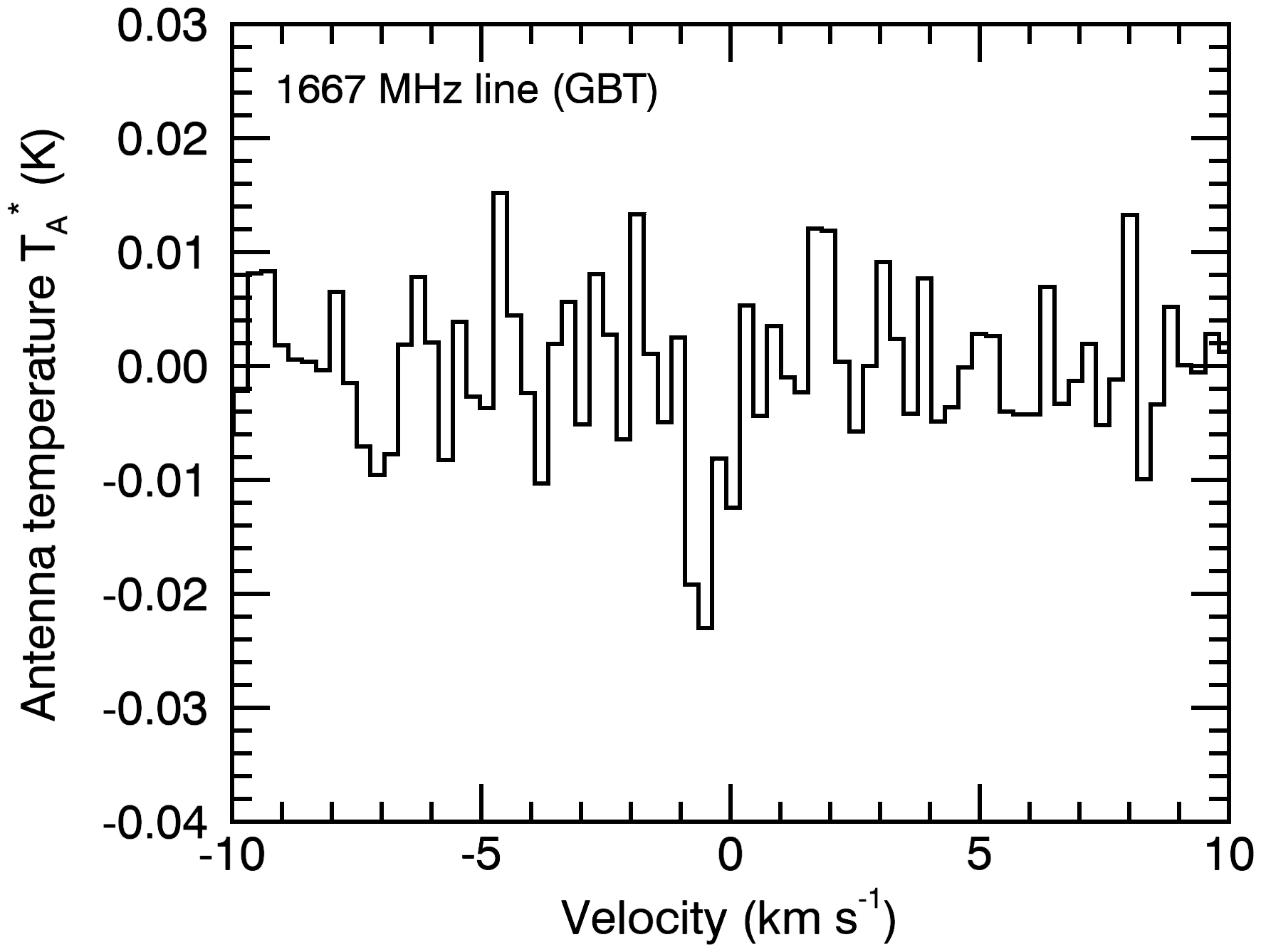
Figure 3: OH $1\leavevmode\nobreak\ 667$ MHz line observed with the GBT on 11.88 August 2020.

2.3 Nançay Radio Telescope observations

Figure 4: Weighted averages of the OH $1\leavevmode\nobreak\ 665$ and $1\leavevmode\nobreak\ 6657$ MHz lines observed at the NRT, normalized to the intensity of the $1\leavevmode\nobreak\ 667$ MHz (Section 2.3). The spectra are integrated over specified periods of time, which are indicated above the plots in yymmdd format. The observations are fitted with trapeziums based on the methodology of Bockelée-Morvan et al. (1990).

Comet F3 was scheduled at the NRT as a Target of Opportunity (ToO) for observations beginning 1 June 2020 and continuing until 27 July 2020. It was observed almost every day during this period, except for 4-17 July 2020 (Table 4). The instrumental characteristics, observing protocol, and data reduction procedure are the same as those used in preceding cometary observations with the NRT. These are described in Crovisier et al. (2002a) and Crovisier et al. (2002b). The NRT is a Meridian telescope, which can observe a given source for $\sim 1$ h. Its RA$\times$Dec beam size is $3.5$′$\times 19$′and its sensitivity is $0.85$ K Jy^-1 at the 18-cm wavelength. The spectrometer, which can accommodate $8$ banks with each having a $195$ kHz bandwidth and $1\leavevmode\nobreak\ 024$ channels, was aimed at the four OH transitions at $1\leavevmode\nobreak\ 665$ and $1\leavevmode\nobreak\ 667$ MHz (main lines) and $1\leavevmode\nobreak\ 612$ and $1\leavevmode\nobreak\ 721$ MHz (satellite lines) in, both, left- and right-hand circular polarizations with a $0.4$ kHz ($0.07$ km s^-1 at $1\leavevmode\nobreak\ 666.0$ MHz) spectral resolution after Hanning smoothing.

Fig. 4 shows the NRT spectra averaged over a few days that were used for kinematic studies based on the line shapes. The depicted spectra are averages of both polarizations and weighted averages of the $1\leavevmode\nobreak\ 665$ and $1\leavevmode\nobreak\ 667$ MHz main lines, converted to the $1\leavevmode\nobreak\ 667$ MHz intensity scale by assuming the statistical ratio of $1.8$. The satellite $1\leavevmode\nobreak\ 612$ MHz line is clearly detected in the NRT data averaged over the 18-27 July observing window. The spectrum containing the $1\leavevmode\nobreak\ 720$ MHz satellite line is noisier; and the detection is only marginal. The four OH $18$-cm lines observed in comet F3 with the NRT averaged from 18 to 27 July 2020 are shown in Fig. 8. The expected statistical relative intensities of the $1\leavevmode\nobreak\ 667:1\leavevmode\nobreak\ 665:1\leavevmode\nobreak\ 612:1\leavevmode\nobreak\ 720$ MHz lines are $9:5:1:1$, which is in good agreement with the observations. The satellite OH lines were tentatively detected at the $1\sigma$ level on 31.8 July 2020 with the $\sim 3\arcmin$ circular beam (at $1\leavevmode\nobreak\ 667$ MHz) of the Arecibo Telescope (Smith et al., 2021).

The NRT spectra of 24.61 July 2020 were recorded nearly simultaneously with the Day 1 GBT observation and are analyzed individually in Section 3.1.3 (sixth line of Table 4). The $1\leavevmode\nobreak\ 665$ and $1\leavevmode\nobreak\ 667$ MHz spectra observed on this date are shown in Fig. 2. The measured $1\leavevmode\nobreak\ 667/1\leavevmode\nobreak\ 665$ MHz line integrated intensity ratio is $1.82\pm 0.13$, which is consistent within uncertainties with the statistical ratio of $1.8$. The other daily spectra are not shown individually. However, in Table 4, daily measurements for July are provided, alongside averages over a few days in June and July. For the dates in June, it was not possible to compute the OH production rate on a daily basis due to the relative weakness of the OH lines (due to a larger geocentric distance). Of particular importance is the entry for 2 July 2020 with its high maser inversion ($i<-0.31$), which allowed the OH production rate near perihelion to be estimated (Section 3.1.5).

3 Results

3.1 OH data analysis

3.1.1 Model for OH production rate determination

In comets, the excitation of OH through UV pumping and subsequent fluorescence leads to population inversion (or anti-inversion) in the sublevels of the $\Lambda$-doublet of the ${}^{2}\Pi_{3/2}\leavevmode\nobreak\ J=3/2$ ground-state. The population inversion ($i$) depends strongly on the comet heliocentric velocity and has been modeled by Despois et al. (1981) and Schleicher & A’Hearn (1988). Depending on the sign of $i$, the four hyperfine components of the $\Lambda$-doublet appear in either emission or absorption. The velocity-integrated flux density (i.e., line area) can be expressed as (e.g., Despois et al., 1981; Schloerb & Gérard, 1985):

$$\int S_{\nu}dv=\frac{A_{\rm ul}kcT_{\rm bg}}{4\pi\Delta^{2}}\frac{2F_{u}+1}{8}\Big{[}i+\frac{i+1}{2}\frac{h\nu}{kT_{\rm bg}}\Big{]}\leavevmode\nobreak\ \Gamma_{\rm OH}.$$ (1)

In this equation, $A_{\rm ul}$ is the Einstein spontaneous coefficient of the line at frequency $\nu$, $F_{\rm u}$ is the statistical weight of the upper level of the transition ($F_{\rm u}=1$ and $2$ for the $1\leavevmode\nobreak\ 667$ and $1\leavevmode\nobreak\ 665$ MHz lines, respectively), $i$ is the inversion of the ground state $\Lambda$-doublet levels, $T_{\rm bg}$ is the background temperature, and $\Delta$ is the Earth-comet distance. $\Gamma_{\rm OH}$ is the number of molecules within the beam, which is proportional to the OH production rate ($Q_{\rm OH}$). The second term inside the brackets corresponds to spontaneous emission and is only significant for small values of $i$. For the 100-m GBT, the area of the $1\leavevmode\nobreak\ 667$ MHz line, expressed in K km s^-1 on the main beam brightness temperature scale, is given by:

$$\int T_{\rm mB}dv=9.157\times 10^{-35}\frac{T_{\rm bg}}{{\Delta^{2}}}\Big{[}i+\frac{i+1}{2}\frac{h\nu}{kT_{\rm bg}}\Big{]}\leavevmode\nobreak\ \Gamma_{\rm OH},$$ (2)

where the geocentric distance is in astronomical units.

In the inner part of the coma, collisions thermalize the populations of the $\Lambda$-doublet and quench the signal. Based on 1P/Halley observations, Gérard (1990) showed that the quenching radius (in km) can be approximated by:

$$r_{\rm q}=4.7\times 10^{4}r_{\rm h}\sqrt{Q_{\rm OH}/10^{29}},$$ (3)

where $Q_{\rm OH}$ is the OH production rate in molec s^-1. For an active comet such as F3, the quenched region can be expected to be comparable to the projected field of view, which is $2.29\times 10^{5}$ km in diameter for the GBT and $\left(1.07\times 10^{5}\right)\times\left(5.80\times 10^{5}\right)$ km for the NRT on 24 July 2020. Hence, collisional quenching is an important factor to consider when deriving OH production rates from the GBT and NRT observations of comet F3. The nearly simultaneous observations (a mere $2$ hours apart) of the comet by these two instruments provide a new opportunity to measure the quenching radius. The very few prior measurements are based on the comparison of 18-cm- and UV-derived OH production rates (Gérard, 1990) and on the analysis of 18-cm observations taken at various offset positions from the comet nucleus (Colom et al., 1999; Schloerb et al., 1997; Gérard et al., 1998).

In order to take into account collisional quenching, it is assumed that the maser inversion is zero for cometocentric distances $r\leq r_{\rm q}$, following Schloerb (1988) and Gérard (1990). More realistic descriptions with a progressive quenching throughout the coma have been investigated by Colom et al. (1999) and Gérard et al. (1998). Equations 1-2 are then no longer valid, but can be replaced by similar equations: $\Gamma_{\rm OH}$ is replaced by the number of unquenched OH radicals within the beam and only the spontaneous emission term (with $i=0$) is considered for the OH radicals within the quenched region. Despois et al. (1981) have shown that in the collisional region the maser inversion is very small, that is on the order of $10^{-4}$ for a kinetic temperature of $300$ K; thus, it can be safely neglected for the purpose of our analysis of comet F3. The calculation of the number of quenched and unquenched OH radicals within the beam is done by volume integration within a Gaussian beam using a description of the distribution of the OH radicals in the coma (see, e.g., Despois et al., 1981).

For the spatial distribution of the OH radicals, the Haser-equivalent model is employed (Combi & Delsemme, 1980). The water and OH radical lifetimes at $1$ au from the Sun are set to $8.5\times 10^{4}$ (for the quiet Sun from Crovisier 1989, considering that the Sun was quiet in summer 2020) and $1.1\times 10^{5}$ s (van Dishoeck & Dalgarno 1984, but poorly constrained as discussed in Schloerb & Gérard 1985), respectively (see also table $3$ in Crovisier et al. 2002a). The OH ejection velocity is set to $v_{\rm e}=0.95$ km s^-1 (Bockelée-Morvan et al., 1990; Crovisier et al., 2002a). The OH parent velocity $v_{\rm p}$ is derived from the OH line profile, as described in Section 3.1.2.

Table 3: GBT observations: line intensities and spectral characteristics.

UT Date	$\Delta$	$r_{\text{h}}$	Line	RMS(1)	Area ($T_{\text{A}}^{*})^{(2)}$	Width(3)	$\Delta v^{(3)}$	$v_{p}$+$v_{e}^{(4)}$
(yyyy/mm/dd)	(au)	(au)		(mK channel-1)	(K km s-1)	(km s-1)	(km s-1)	(km s-1)
2020$/$07$/$24.71	0.696	0.667	OH $1\leavevmode\nobreak\ 665$	$12$	$0.428\pm 0.014$	$2.89\pm 0.11$	$-0.07\pm 0.05$	$2.32\pm 0.07$
2020$/$08$/$11.88	1.078	1.053	OH $1\leavevmode\nobreak\ 665$	$9$	$<0.03$	–	–	–
2020$/$07$/$24.71	0.696	0.667	OH $1\leavevmode\nobreak\ 667$	$10$	$0.827\pm 0.012$	$2.95\pm 0.05$	$-0.05\pm 0.02$	$2.43\pm 0.04$
2020$/$08$/$11.88	1.078	1.053	OH $1\leavevmode\nobreak\ 667$	$9$	$-0.017\pm 0.005$	$0.67\pm 0.27$	$-0.53\pm 0.12$	–
2020$/$07$/$24.81	0.696	0.669	NH3 ($1_{1}-1_{1}$)	$48$	$<0.017$	–	–	–
2020$/$07$/$24.81	0.696	0.669	NH3 ($2_{2}-2_{2}$)	$47$	$<0.016$	–	–	–
2020$/$07$/$24.81	0.696	0.669	NH3 ($3_{3}-3_{3}$)	$47$	$<0.016$	–	–	–
2020$/$07$/$24.81	0.696	0.669	NH3 ($4_{4}-4_{4}$)	$46$	$<0.016$	–	–	–
2020$/$07$/$24.81	0.696	0.669	NH3 ($5_{5}-5_{5}$)	$46$	$<0.016$	–	–	–

⁽¹⁾ For a spectral channel width of $\sim 0.005$ km s^-1 for the NH₃ lines and $\sim 0.3$ km s^-1 for the OH $1\leavevmode\nobreak\ 665$ and $1\leavevmode\nobreak\ 667$ MHz lines.
⁽²⁾ Velocity-integrated flux density (i.e., line area) in the $T_{\text{A}}^{*}$ scale or a $3\sigma$ upper limit. Considered velocity intervals are $\left[-2.5,+2.5\right]$ km s^-1 and $\left[-1.5,1.5\right]$ km s^-1 for the OH and NH₃ lines, respectively. For the OH $1\leavevmode\nobreak\ 667$ MHz line observed on 11.88 August 2020, the line area is that obtained from a Gaussian fit.
⁽³⁾ Velocity offset from a Gaussian fit.
⁽⁴⁾ Half lower bases of the fitted trapezia (Fig. 2).

Table 4: OH observations at NRT: line intensities and spectral characteristics.

UT Date	$\Delta$	$r_{\text{h}}$	$v_{\text{h}}$	$i^{(1)}$	$i^{(2)}$	$T_{\text{bg}}$	Area(3)	$\Delta v^{(4)}$	$v_{p}+v_{e}^{(5)}$	$Q_{\text{OH}}^{(1)}$	$Q_{\text{OH}}^{(2)}$
(yyyy/mm/dd)	(au)	(au)	(km s-1)			(K)	(mJy km s-1)	(km s-1)	(km s-1)	($10^{29}$ molec s-1)	($10^{29}$ molec s-1)
				(Des)	(Sch)					(Des)	(Sch)
2020/07/02.46	1.19	0.30	$-7.2$	$-0.31$	$-0.37$	3.4	$-30\pm 13$	–	–	$18.6\pm 4.8$	$22.0\pm 4.8$
2020/07/18.54	0.72	0.53	38.5	0.20	0.28	3.1	$526\pm 32$	$-0.41\pm 0.14$	–	$21.4\pm 3.8^{(6)}$	$8.47\pm 1.17^{(6)}$
2020/07/19.55	0.71	0.55	38.7	0.22	0.30	3.1	$379\pm 32$	$-0.13\pm 0.16$	–	$6.03\pm 0.93^{(6)}$	$3.69\pm 0.48^{(6)}$
2020/07/20.56	0.70	0.57	38.8	0.23	0.30	3.1	$491\pm 35$	$-0.33\pm 0.13$	–	$8.81\pm 1.62^{(6)}$	$5.14\pm 0.69^{(6)}$
2020/07/23.60	0.69	0.64	38.6	0.21	0.29	3.1	$402\pm 20$	$-0.07\pm 0.09$	–	$5.13\pm 0.53^{(6)}$	$3.00\pm 0.23^{(6)}$
2020/07/24.61	0.70	0.66	38.5	0.20	0.28	3.1	$414\pm 23$	$-0.12\pm 0.09$	$2.25\pm 0.14$	$4.62\pm 0.38$	$3.41\pm 0.25$
2020/07/26.63	0.71	0.71	38.2	0.17	0.25	3.1	$359\pm 19$	$+0.05\pm 0.10$	–	$5.15\pm 0.59^{(6)}$	$2.71\pm 0.23^{(6)}$
2020/07/27.63	0.72	0.73	38.0	0.15	0.23	3.1	$279\pm 19$	$-0.10\pm 0.11$	–	$3.79\pm 0.47^{(6)}$	$2.02\pm 0.20^{(6)}$
2020/06/01-2020/06/12	1.58	0.79	$-37.5$	$-0.24$	$-0.26$	3.4	$-115\pm 5$	$-0.09\pm 0.06$	$2.44\pm 0.08$	$2.32\pm 0.12$	$2.10\pm 0.11$
2020/06/14-2020/06/24	1.47	0.52	$-37.7$	$-0.25$	$-0.26$	3.5	$-165\pm 5$	$-0.20\pm 0.07$	$2.79\pm 0.11$	$8.00\pm 0.49$	$7.32\pm 0.50$
2020/07/02-2020/07/03	1.18	0.30	$-4.8$	$-0.23$	$-0.28$	3.4	$-49\pm 10$	–	–	–	–
2020/07/18-2020/07/20	0.71	0.55	38.6	0.21	0.29	3.1	$459\pm 19$	$-0.28\pm 0.08$	$2.72\pm 0.12$	$10.0\pm 1.1$	$5.30\pm 0.37$
2020/07/23-2020/07/24	0.69	0.65	38.6	0.21	0.29	3.1	$409\pm 14$	$-0.09\pm 0.06$	$2.35\pm 0.10$	$5.03\pm 0.34$	$3.03\pm 0.17$
2020/07/26-2020/07/27	0.72	0.72	38.1	0.16	0.24	3.1	$322\pm 13$	$-0.02\pm 0.08$	$1.94\pm 0.05$	$4.62\pm 0.41$	$2.40\pm 0.15$

⁽¹⁾ Maser inversion from Despois et al. (1981) and corresponding inferred OH production rate.
⁽²⁾ Maser inversion from Schleicher & A’Hearn (1988) and corresponding inferred OH production rate.
⁽³⁾ Weighted average of the $1\leavevmode\nobreak\ 667$ and $1\leavevmode\nobreak\ 665$ MHz lines converted to the $1\leavevmode\nobreak\ 667$ MHz intensity scale, assuming the statistical ratio of $1.8$.
⁽⁴⁾ Velocity offset from a Gaussian fit.
⁽⁵⁾ Half lower bases of the fitted trapezia (Figs. 2 and 4).
⁽⁶⁾ Trapezium fitting was not performed for this date. The assumed $v_{p}$ value is that deduced from the $r_{\text{h}}$ evolution of $v_{p}$ measured from the $2-3$ day averages over the $18-27$ July 2020 period.

3.1.2 Line profiles and H₂O outflow velocity

The observed line shapes have been analyzed in the framework of the trapezium modeling as proposed by Bockelée-Morvan et al. (1990) and subsequently applied to the kinematic studies of the coma of many comets in Tseng et al. (2007). OH is a daughter species of H₂O photodissociation and is assumed here to be emitted isotropically in the rest frame of H₂O. Indeed, some anisotropy may occur since water photodissociation is caused by the unidirectional solar UV radiation (e.g., Crovisier 1990). However, the currently available theoretical work and laboratory data do not permit a complete evaluation of this potential anisotropy. Taking into account collisional quenching, the line width of OH does not provide the velocity of its parent molecule. The maximum radial velocity of OH along the line of sight is $v_{\rm p}$+$v_{\rm e}$, assuming that the OH parent and OH ejection velocity distributions are monokinetic. A trapezium centered on the cometary nucleus is expected when the beam is very large with respect to the OH coma. As shown by Bockelée-Morvan et al. (1990), the half lower base of the fitted trapezium to an OH line is expected to be equal to $v_{\rm p}$+$v_{\rm e}$. Figs. 2 and 4 show the trapezium method applied to the GBT and NRT OH spectra. The derived $v_{\rm p}$+$v_{\rm e}$ values are given in Tables 3 and 4.

The OH parent velocity derived from the GBT $1\leavevmode\nobreak\ 667$ MHz line observed on 24 July 2020 is $v_{\rm p}=1.48\pm 0.04$ km s^-1. The trapezium method applied to the Nançay spectrum of 24 July 2020 yields $v_{\rm p}$ = 1.30 $\pm$ 0.14 km s^-1, which is consistent within $1\sigma$ with the GBT-derived value. A slightly lower $v_{\rm p}$ value measured at NRT is not unexpected, as it could be explained by gas acceleration in the coma. With its $3.5\arcmin\times 19\arcmin$ beam, the NRT field of view is probing OH radicals closer to the surface than the $7.55\arcmin$ GBT beam (at $1\leavevmode\nobreak\ 667$ MHz). As expected, the OH parent expansion velocity $v_{\rm p}$ is observed to increase from $\sim 1.0$ to $\sim 1.8$ km s^-1 when the heliocentric distance $r_{\rm h}$ decreases from $\sim 0.72$ to $\sim 0.52$ au (Table 4). This trend was observed in other comets (Tseng et al., 2007).

3.1.3 Combined analysis of the GBT and NRT OH observations of 24 July 2020

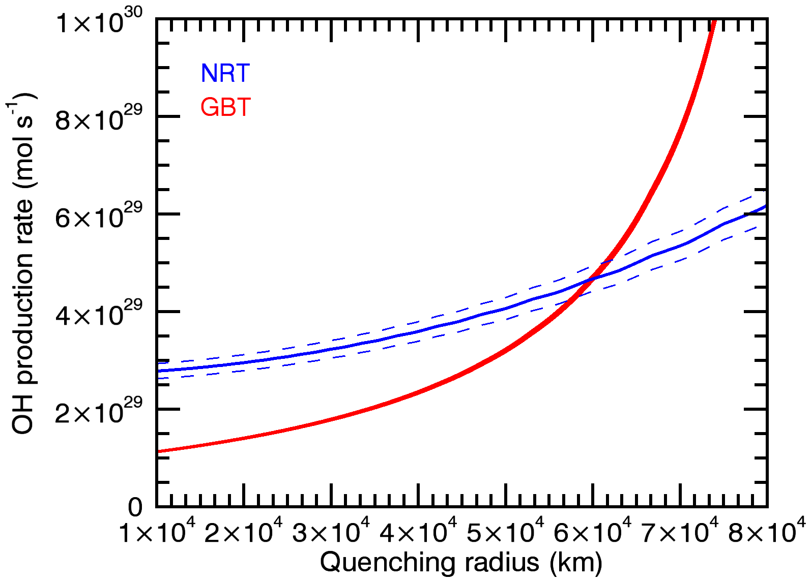
Figure 5: Derived OH production rates from the GBT (red curve) and NRT (blue curves) observations of the OH $1\leavevmode\nobreak\ 667$ MHz line in comet C/2020 F3 (NEOWISE) on 24 July 2020. OH production rates are plotted as a function of the quenching radius. The dashed lines correspond to the $\pm 1\sigma$ uncertainty in the line area measured at NRT. Analogous dashed lines for the GBT are indistinguishable from the solid curve due to the high signal-to-noise ratio of the data. The maser inversion is $i=0.20$ based on Despois et al. (1981), and the background temperature is $T_{\text{bg}}=3.1$ K. The OH spatial distribution is described by the Haser-equivalent model (Combi & Delsemme, 1980).

Due to the significant differences in beam sizes and shapes between the GBT and NRT (of a factor of about two considering the small dimension of the NRT’s elliptical beam), the fractions of quenched OH radicals that the two telescopes sample differ. The quenching radius $r_{\rm q}$ can be determined by searching for the $Q_{\rm OH}$ value that is consistent with data from both facilities. Fig. 5 shows $Q_{\rm OH}$ values derived as a function of $r_{\rm q}$ from the 24 July 2020 GBT and NRT data using the maser inversion of $i=0.20$ based on Despois et al. (1981). For the GBT and NRT calculations, the derived $v_{\rm p}=1.48$ km s^-1 and $v_{\rm p}=1.30$ km s^-1 values are utilized, respectively (Section 3.1.2). The obtained quenching radius is $\left(5.95\pm 0.14\right)\times 10^{4}$ km and the consistent OH production rate is $\left(4.62\pm 0.38\right)\times 10^{29}$ molec s^-1. Using the maser inversion $i=0.28$ based on Schleicher & A’Hearn (1988), the derived $r_{\rm q}$ value is the same ($\left(5.96\pm 0.14\right)\times 10^{4}$ km), but the OH production rate is $\left(3.41\pm 0.25\right)\times 10^{29}$ molec s^-1. The derived quenching radius is consistent with the law provided by Eq. 3, which predicts values of $5.6\times 10^{4}$ and $6.6\times 10^{4}$ km for the two obtained $Q_{\rm OH}$ values. Averaging the production rates inferred with the Despois et al. (1981) and Schleicher & A’Hearn (1988) maser inversion ($i$) models yields an OH production rate of $\left(4.02\pm 0.32\right)\times 10^{29}$ molec s^-1, which is consistent with each model individually within errors. The corresponding averaged water production rate is $\left(4.42\pm 0.35\right)\times 10^{29}$ molec s^-1. The two considered maser inversion models were developed independently and compared in Schloerb & Gérard (1985). The two models use different sources for the solar spectrum. The model of Schleicher & A’Hearn (1988) includes IR pumping (a minor effect). Both models give remarkably similar results, except when the OH inversion is low.

3.1.4 GBT spectrum of 11 August 2020

The GBT on-nucleus data obtained on 11 August 2020 show a marginal absorption line near the frequency of the OH $1\leavevmode\nobreak\ 667$ MHz line at the nucleus-centered beam position (Fig. 3). Unlike the 24 July 2020 spectrum, the line is narrow ($\sim 1$ km s^-1), strongly blueshifted ($\Delta v=-0.53$ km s^-1 from a Gaussian fit, Table 2), and does not show any signal at positive Doppler velocities. This line shape can be explained by the Greenstein effect (Greenstein, 1958). As a result of the motion of the OH radicals in the coma, their heliocentric velocity is shifted with respect to the nucleus heliocentric velocity, adding another component to the maser inversion (Despois et al., 1981). In most instances, the Greenstein effect only affects weakly the shape of the OH lines. However, the effect is striking at heliocentric velocities where the maser inversion changes its sign over a small velocity range, since some radicals have a positive maser inversion, and others have a negative inversion.

The heliocentric velocity of comet F3 at the time when the GBT observations of 11 August 2020 were carried out was $v_{\text{h}}=+34.8$ km s^-1. For the Despois et al. (1981) model, the maser inversion is $i=-0.125$ at this $v_{\text{h}}$, but varies from $-0.240$ to $+0.006$ in the coma assuming that the maximum OH expansion velocity ($v_{\rm p}$+$v_{\rm e}$) is $2$ km s^-1. For the Schleicher & A’Hearn (1988) model, the inversion is in the $\left[-0.16,+0.09\right]$ range with $i=-0.020$ at this value of $v_{\text{h}}$. Taking into account the Sun-comet-Earth angle of $58.8^{\circ}$ (phase angle) and spontaneous emission, it is expected that the line will be in absorption at negative Doppler velocities and will show at positive velocities either weak positive or negative emission depending on the Schleicher et al. or the Despois et al. inversion values, respectively. The low signal-to-noise ratio prevents any conclusion about which model is in better accordance with the observed spectrum.

Equations 1-2 hold in the presence of the Greenstein effect, so they have been used for an attempt to determine the OH production rate on 11 August 2020. For this, the quenching law given by Eq. 3, $T_{\rm bg}=3.1$ K, and $v_{\rm p}=1.2$ km s^-1 have been employed. This $v_{\rm p}$ value is calculated from the value of $1.48$ km s^-1 determined on 24 July (Table 3) and an assumed a $r_{\text{h}}^{-0.5}$ dependence. The Schleicher et al. excitation model cannot explain the observed line intensity (Table 3) with this quenching law. A value of $Q_{\rm OH}$ in the $0.5-3\times 10^{29}$ molec s^-1 range is obtained using the Despois et al. inversion value. If the quenching radius is left as a free parameter, the derived $Q_{\rm OH}$ strongly depends on $r_{\rm q}$ and $i$ values. It becomes necessary to conclude that it is not possible to derive a reliable $Q_{\rm OH}$ value from the 11 August 2020 data. The $1\leavevmode\nobreak\ 665$ MHz spectrum and the $1\leavevmode\nobreak\ 665$, $1\leavevmode\nobreak\ 667$ MHz spectra obtained at offset positions do not show even any marginal hints of lines and were not analyzed.

3.1.5 Evolution of the OH production rate

Table 4 presents the OH production rates determined from the NRT data using the Despois et al. (1981) and the Schleicher & A’Hearn (1988) inversion models. The average spectrum of 2-3 July 2020 observations shows an absorption line consistent with the inversion models. The maser inversion was very low on 3 July 2020. Consequently, as for the GBT data of 11 August 2020 (Section 3.1.4), this observation could not be used for determining a production rate. On the other hand, an OH production rate of $\sim 2\times 10^{30}$ molec s^-1 could be determined for 2 July (i.e., one day before perihelion; Table 4). Despite the maser inversion being large on this date (either $-0.31$ or $-0.37$ depending on the inversion model), the signal was weak due to a large fraction of quenched OH radicals in the beam.

The OH 18-cm lines were observed in emission with the Arecibo 305-m dish on 31.8 July 2020 ($r_{\rm h}=0.82$ au), from which an unexpectedly low OH production rate of $\left(3.6\pm 0.6\right)\times 10^{28}$ molec s^-1 was derived (Smith et al., 2021). However, collisional quenching was not taken into account in the analysis presented in that paper. In this work, the Arecibo data were reanalyzed with collision quenching being taken into account. The inferred values are $Q_{\rm OH}=\left(1.5\pm 0.3\right)\times 10^{29}$ molec s^-1 with the inversion model of Despois et al. (1981) and $\left(2.95\pm 0.05\right)\times 10^{29}$ molec s^-1 with that of Schleicher & A’Hearn (1988). These values are in much closer agreement with the production rate estimated from optical OH line observations for the same observation date of $8.5\times 10^{28}$ molec s^-1 quoted in the Smith et al. (2021) paper (based on D. Schleicher 2021, personal communication).

The derived water production rates ($Q_{\text{H}_{2}\text{O}}=1.1\times Q_{\rm OH}$; Crovisier 1989) are plotted in Fig. 6 together with other water production rate determinations from near-IR water lines observed with long-slit spectroscopy with the iSHELL at NASA/IRTF (Faggi et al., 2021) and from Ly-$\alpha$ observations using SOHO/SWAN (Combi et al., 2021). There is a good agreement between the OH 18-cm and Ly-$\alpha$ $Q_{\text{H}_{2}\text{O}}$ data post-perihelion, but a factor of two discrepancy is observed pre-perihelion. Understanding this is potentially important, but requires dedicated modeling efforts that are beyond the scope of this paper. Near-IR determinations, which were all obtained post-perihelion (see red symbols in Fig. 6), are overall consistent with the OH 18-cm for contemporaneous dates. The large discrepancy between near-IR and Ly-$\alpha$ measurements near-perihelion ($r_{\rm h}<0.4$ au) is discussed in Faggi et al. (2021) and may be related to an extended production of water, for example, from icy grains. Generally, robust comparisons across the UV, IR, and radio domains are challenging due to the significantly different spatial scales being probed (FOV of $30^{\circ}$, $0.3-4\arcsec$, and $32\arcsec-19\arcmin$, respectively).

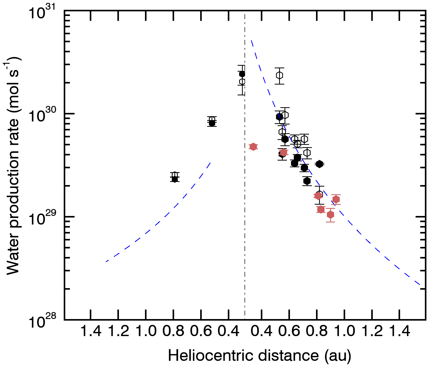
Figure 6: Water production rates of comet C/2020 F3 (NEOWISE). Black dots are values from this work and include the revised value from the Arecibo data: filled and open dots refer to values obtained with the inversion models of Schleicher & A’Hearn (1988) and Despois et al. (1981), respectively. Red dots: values from near-IR observations from Faggi et al. (2021). The dashed blue lines are a fit to the pre- and post-perihelion heliocentric values derived from Ly-$\alpha$ data (Combi et al., 2021).

3.2 NH₃ data analysis

The analysis of the NH₃ lines was performed using the excitation model described in Biver et al. (2012). Since the NH₃ photodissociation lifetime is short ($\sim 2\leavevmode\nobreak\ 700$ s at $r_{\text{h}}=0.7$ au) and the water production rate of comet F3 is high, the excitation of NH₃ is dominated by collisional processes and its rotational levels are in thermal equilibrium. A gas kinetic temperature of $90$ K is assumed, based on constraints from close-in-date CH₃OH observations of this comet at the IRAM $30$-m and NOEMA telescopes (Biver et al., 2022a). An expansion velocity of $1$ km s^-1 is utilized, as derived from the line profiles observed at IRAM $30$-m and NOEMA, which is appropriate as the field of view ($9-34\arcsec$) of these observations matches the size of the expected NH₃ coma.

The NH₃ lines at $23-25$ GHz present a hyperfine structure with several components that are well-separated (by more than $7$ km s^-1) from the central frequencies of the lines (as can be seen in the Cologne Database of Molecular Spectroscopy, CDMS, Müller et al. 2001, 2005; Endres et al. 2016). Each of these components, in turn, harbors closely spaced (by less than $0.03$ km s^-1) quadrupole satellite lines. Two to three such satellite components contribute to the signal in the velocity interval from $-1.5$ to $1.5$ km s^-1 that is chosen for computing the NH₃ line areas in Table 3. The fraction of the intensity in the central hyperfine components is $50/80/89/93/96\leavevmode\nobreak\ \%$ for the $J_{K}=1_{1}-1_{1}/2_{2}-2_{2}/3_{3}-3_{3}/4_{4}-4_{4}/5_{5}-5_{5}$ lines (which can be computed based on the CDMS spectroscopic entry). With this taken into consideration, the modeled line strengths show that the $J_{K}=2_{2}-2_{2}$ and $3_{3}-3_{3}$ lines are, by far, the major contributors to the expected signal in this velocity interval. Based on these two lines and an RMS^-2 weighting, the resulting $3\sigma$ upper limit on the NH₃ production rate is $Q_{\text{NH}_{3}}<1.3\times 10^{27}$ molec s^-1. Using the water production rate of $4.4\times 10^{29}$ molec s^-1 inferred from OH observations on 24 July 2020 (Section 3.1.3, an average of the Despois et al. (1981) and Schleicher & A’Hearn (1988) maser inversion models), the resulting $3\sigma$ upper limit for $Q_{\text{NH}_{3}}/Q_{\text{H}_{2}\text{O}}$ is $<0.29\%$.

Faggi et al. (2021) detected near-IR lines of NH₃ in comet F3 and derived NH₃ abundances relative to water of $0.73\pm 0.10\%$ (on 31 July 2020 at $r_{\text{h}}=0.81$ au, $Q_{\text{H}_{2}\text{O}}=(1.6\pm 0.05)\times 10^{29}$ molec s^-1) and $0.92\pm 0.19\%$ (on 6 August 2020 at $r_{\text{h}}=0.94$ au, $Q_{\text{H}_{2}\text{O}}=(1.5\pm 0.2)\times 10^{29}$ molec s^-1). The discrepancy with our value is puzzling. The measurements of NH₃ in Faggi et al. (2021) were usually performed on one or two very faint spectral lines, which prevented a direct derivation of $T_{\text{rot}}$. Consequently, it was assumed that $T_{\text{rot}}(\text{NH}_{3})=T_{\text{rot}}(\text{H}_{2}\text{O})$. Based on near-IR H₂O observations, the rotational temperature was derived to be $130$ K on 20 July and $90$ K on 31 July. If for the analysis of the GBT NH₃ lines, a $T_{\text{rot}}$ of $130$ K is assumed, then the $3\sigma$ upper limit on the NH₃ production rate is $Q_{\text{NH}_{3}}<1.4\times 10^{27}$ molec s^-1 (based on the $J_{K}=2_{2}-2_{2}$ and $3_{3}-3_{3}$ lines and a RMS^-2 weighting). This is $\sim 11\%$ higher than with a $T_{\text{rot}}$ of $90$ K; however, still not enough to explain the discrepancy with the near-IR values. Possibly, NH₃ displayed abundance variations with time. An increase in abundance relative to H₂O with increasing $r_{\text{h}}$ was observed for CH₃OH, C₂H₆, and CH₄ species in these near-IR observations, while abundances of HCN, C₂H₂, and H₂CO were stable relative to H₂O (Faggi et al., 2021). On the other hand, increases relative to H₂O with increasing $r_{\text{h}}$ were not observed for CH₃OH nor H₂CO in the IRAM $30$-m data (Biver et al., 2022a).

It is not likely that the water production rate has been strongly overestimated in this work, thereby resulting in a low $Q_{\text{NH}_{3}}/Q_{\text{H}_{2}\text{O}}$ ratio. For the 24 July 2020 date in question ($r_{\text{h}}=0.7$ au), here a $Q_{\text{H}_{2}\text{O}}=\left(4.42\pm 0.35\right)\times 10^{29}$ molec s^-1 is used (Section 3.1.3). Unfortunately, near-IR measurements are not available for this exact date. For 20 July 2020 ($r_{\text{h}}=0.56$ au), Faggi et al. (2021) obtain $(4.2\pm 0.2)\times 10^{29}$ molec s^-1, whereas the $Q_{\text{H}_{2}\text{O}}$ value obtained from radio OH observation on this date is $\left(6.3\pm 0.7\right)\times 10^{29}$ molec s^-1 (weighted average of values deduced using the two maser inversion models, Table 4). Hence, the OH-derived value is only slightly (factor of $1.5$) larger than the IR-derived value. If $Q_{\text{H}_{2}\text{O}}$ was a factor of $1.5$ lower than what has been obtained in the current analysis on 24 July 2020, the upper limit for $Q_{\text{NH}_{3}}/Q_{\text{H}_{2}\text{O}}$ would increase to $<0.44\%$, which is still well below the ratio obtained from near-IR.

The OH that is observed in comet F3 at $r_{h}=0.7$ au stems predominantly from H₂O that has exited the nucleus between $\sim 4\times 10^{4}$ s ($\sim 12$ h, lifetime of water) and $\sim 8\times 10^{4}$ s ($\sim 22$ h, time for the OH radicals to reach a distance corresponding to the projected GBT beam radius) earlier. On the other hand, NH₃ would be freshly released and would not survive for more than $\sim 2.7\times 10^{3}$ s ($\sim 45$ min). There is no evidence for strong daily variability in $Q_{\text{H}_{2}\text{O}}$ in the radio observation presented nor when they are compared to the near-IR observation of (Faggi et al. 2021, Fig. 6). Consequently, the discrepancy between near-IR and radio determinations of $Q_{\text{NH}_{3}}/Q_{\text{H}_{2}\text{O}}$ may be related to the temporal variability of $Q_{\text{NH}_{3}}$.

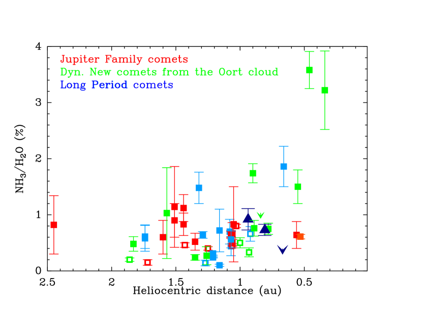
Figure 7: NH₃ abundances relative to water measured in comets from centimeter and submillimeter observations (hollow symbols), and near-IR observations (filled symbols). Different colors are used for Jupiter-family comets, dynamically new comets from the Oort Cloud, and long-period comets originating from the Oort Cloud. Downward-pointing arrowheads are $3\sigma$ upper limits. Dark blue upward-pointing triangles refer to the measurements of comet F3 from Faggi et al. (2021). The dark blue downward-pointing arrowhead is the value derived in this work. All data used for this figure are tabulated in Tables 5 and 6 with the corresponding references.

4 Discussion

Comet F3 was supposed to be a prime target for the investigation of the evolution of the NH₃/H₂O ratio as a function of heliocentric distance. It boasted a high water production rate ($>10^{30}$ molec s^-1 around perihelion), which was firmly quantified during the two month-long monitoring of OH with the NRT. Its heliocentric distance at perihelion ($0.295$ au) and geocentric distance at perigee ($0.692$ au) were short. The GBT observational campaign targeted OH and NH₃ near-simultaneously, thereby ensuring robust constraints on the NH₃/H₂O ratio. However, the NH₃ hyperfine inversion lines at $23-25$ GHz eluded detection like for many other comets in the past (Section 1). The NH₃ abundance relative to water was quantified in several preceding comets (Fig. 7) based on detections of NH₃ at $572$ GHz using Odin, Herschel, and Rosetta/MIRO (Biver et al. 2007, 2012, 2019, and unpublished results from N. Biver, personal communication) and in the near-IR (Dello Russo et al. 2016; Lippi et al. 2021, and other references in Table 5). The upper limit obtained for comet F3 (blue downward-pointing arrowhead in Fig. 7) is in the low range of values measured in comets at $0.7$ au from the Sun.

There is a trend for higher NH₃ abundances at low ($<1$ au) heliocentric distances (Fig. 7), suggesting a possible contribution of NH₃ released from the thermal degradation of compounds on grains at small $r_{\rm h}$. This is supported by the radial profiles of NH₃, which are often more extended than expected for a nuclear source of NH₃ (e.g., DiSanti et al., 2016; Dello Russo et al., 2022). A similar increase at low heliocentric distances is also seen in the $Q(\text{NH}_{3})/Q(\text{C}_{2}\text{H}_{6})$ ratio (fig. $5$ of Mumma et al. 2019). The thermal decomposition of ammonium salts discovered in comet 67P/C-G (Quirico et al., 2016; Altwegg et al., 2020; Poch et al., 2020) has been proposed to explain the excess of NH₃ production at small $r_{\rm h}$ (Mumma et al., 2019). This excess of production is not observed for comet F3, based on the here-obtained NH₃/H₂O upper limit and the NH₃ abundance determined in the near-IR (Faggi et al., 2021). A contributing factor could be the amount of water-poor dust launched into the coma of a comet. At $0.7$ au from the Sun, the equilibrium temperature of dust grains is already above the $\sim 160-230$ K threshold for thermal degradation of some ammonium salts. The increase in the NH₃/H₂O ratio must therefore be correlated with a higher dust density in the coma. Furthermore, given enough dust in the coma, an initial grain size distribution can be altered by fragmentation as it moves outward through the coma, which may lead to an increase in the small grain population as a function of distance from the nucleus. The small grains can be super-heated above the equilibrium temperature; whereby, salts with the highest binding energies would also thermally disintegrate. This dust must be dry, i.e., water-poor, because otherwise the amount of H₂O would increase together with NH₃ and potentially mask the increase in the relative abundance of NH₃.

The dust-to-gas ratio in a cometary coma may vary drastically with outbursts. Comet F3 was not observed to undergo outbursts during its 2022 perihelion passage, but rather to only display strong jet activity (Combi et al. 2021, Section 1). Additional observations of NH₃ at low $r_{\rm h}$ are obviously needed. Although, it is not excluded that enhanced NH₃/H₂O ratios may be short-lived as ammonium salts may not survive for long on dust in the coma following an injection of dust from an outburst. Typically, outbursts are more frequent at smaller heliocentric distances, in agreement with the NH₃/H₂O increasing trend. Continuous monitoring pre- and post-outburst would allow the lifetime of ammonium salts in the coma to be estimated.

Several salts have been identified to be present on the surface of 67P/C-G: NH${}^{+}_{4}$Cl^-, NH${}^{+}_{4}$CN^-, NH${}^{+}_{4}$OCN^-, NH${}^{+}_{4}$HCOO^-, NH${}^{+}_{4}$CH₃COO^-, NH${}^{+}_{4}$SH^-, and NH${}^{+}_{4}$F^- (Altwegg et al., 2020, 2022). As ammonium salts degrade at higher temperatures at smaller heliocentric distances, not only the NH₃/H₂O ratio should display an increasing trend, but also the ratio of the acid-counterparts (HCl, HCN, HOCN, HCOOH, HCOOCH₃) relative to H₂O. However, to what extent each of these individual salts makes a significant contribution relative to the amount of these species already present in the ice in the nucleus is not clear. Modeling work is required to quantify these effects. For the case of the CN radical, it has been shown that it does appear to have a distributed source (e.g., Opitom et al. 2016) and requires an additional parent molecule to match its signal strength in the ROSINA measurements of the inner coma of 67P/C-G (Hänni et al., 2020, 2021), thus likely being a product of ammonium salt thermal degradation. This has also been observed for NH₂, a photodissociation product of NH₃ (Opitom et al., 2019). An important step forward would be the comparison of the ¹⁴N/¹⁵N isotopic ratio in the dust with that in various N-bearing volatiles. It has been shown that the ¹⁴N/¹⁵N isotopic ratio for NH₃, NO, N₂ in 67P/C-G is in the $93-160$ range, which is consistent with the $\sim 140$ measured in HCN, CN, and NH₂ in other comets (Altwegg et al., 2019; Bockelée-Morvan et al., 2015; Biver et al., 2022b). This ratio has not been reported for the dust of 67P/C-G.

5 Conclusions

This paper presents the two month-long monitoring campaign of the OH emission from comet C/2020 F3 (NEOWISE) at the Nançay Radio Telescope, which is used to determine the H₂O production rate. Furthermore, GBT observations of F3 targeting OH lines on two separate days (24 July and 11 August 2020) and the NH₃ line observations contemporaneous with the first date are presented. The main results are as follows.

1. The OH parent expansion velocity ($v_{p}$) increases from $1.0$ to $1.8$ km s^-1 with decreasing heliocentric distance from $0.72$ to $0.52$ au.

2. The OH quenching radius ($r_{q}$) is determined to be $\left(5.96\pm 0.10\right)\times 10^{4}$ km on 24 July 2020 ($r_{\text{h}}=0.7$ au) from the analysis of the concurrent NRT and GBT OH observations. This value consistently explains the OH line intensities measured by the GBT and NRT for an OH production rate ($Q_{\text{OH}}$) of $\left(4.02\pm 0.32\right)\times 10^{29}$ molec s^-1. This $r_{q}$ value is consistent with the Gérard (1990) prescription.

3. The Greenstein effect (Greenstein, 1958) is observationally demonstrated in the OH observations of 11 August 2020 taken at the GBT, yielding a narrow, strongly blueshifted line in absorption. The signal-to-noise ratio of the data is not high enough to distinguish between the Despois et al. (1981) and Schleicher & A’Hearn (1988) maser inversion models.

4. One day before perihelion (2 July 2020), the H₂O production rate ($Q_{\text{H}_{2}\text{O}}$) was very high ($\sim 2\times 10^{30}$ molec s^-1) in comet F3. Pre-perihelion, $Q_{\text{H}_{2}\text{O}}$ increases with decreasing heliocentric distance and agrees within a factor of $2$ with Ly-$\alpha$ observations using SOHO/SWAN of Combi et al. (2021). Post-perihelion, $Q_{\text{H}_{2}\text{O}}$ decreases with the increasing heliocentric distance and is in excellent agreement with Ly-$\alpha$ observations.

5. The $3\sigma$ upper limit for $Q_{\text{NH}_{3}}/Q_{\text{H}_{2}\text{O}}$ is $<0.29\%$ for comet F3 at $0.7$ au from the Sun (post-perihelion on 24 July 2020), which is in the low range of values obtained for other comets at similar heliocentric distances.

6. The differences in the $\text{NH}_{3}/\text{H}_{2}\text{O}$ ratios measured for comet F3 with radio and near-IR observations may hint at this ratio being highly variable with time in a cometary coma.

Appendix A Averaged NRT spectra of comet F3 for 18-27 July 2020

Figure 8: Four OH $18$-cm lines observed in comet F3 with the NRT averaged from 18 to 27 July 2020. The expected statistical relative intensities of the $1\leavevmode\nobreak\ 667:1\leavevmode\nobreak\ 665:1\leavevmode\nobreak\ 612:1\leavevmode\nobreak\ 720$ MHz lines are $9:5:1:1$, which is in good agreement with the displayed observations.

Appendix B Ammonia in comets

NH₃ abundances relative to water measured in comets from ground-based radio and IR observations are tabulated in Table 5, while those obtained with in situ measurements are given in Table 6 with the corresponding references. For Fig. 7, all ground-based values have been used from Table 5 except for the measurement for comet C/1995 O1 (Hale-Bopp) from Hirota et al. (1999) due to its large, unconstraining error bars. From Table 6, only the two reported in lines two and three have been used for Fig. 7. The other measurements for comet 67P/Churyumov-Gerasimenko have been tabulated in order to illustrate that a range of values has been measured at this comet over the 2-year duration of the ESA Rosetta mission with two independent instruments: MIRO and ROSINA. The data point of 1P/Halley has been excluded from Fig. 7, because its error bars are large and do not allow for a meaningful comparison.

Table 5: Abundances of ammonia in comets from ground-based observations.

UT date	$r_{h}$	$Q_{\rm NH_{3}}/Q_{\rm H_{2}O}$	Comet		Reference
$($yyyy/mm/dd.d)	(au)	($\%$)	Type	Name
Radio data ($\lambda\sim$cm)
1996 03 24	1.07	$0.44\pm 0.17$	LPC	C/1996 B2 (Hyakutake)	Wootten et al. (1996a, b); Palmer et al. (1996)
					(A. Wootten & B. Butler, pers. comm.)
1997 03 30	0.92	$0.66\pm 0.13$	LPC	C/1995 O1 (Hale-Bopp)	Bird et al. (1997)
1997 04 20	0.98	$1.8\pm 0.9$	LPC	C/1995 O1 (Hale-Bopp)	Hirota et al. (1999)
1997 05 22	1.27	$0.14\pm 0.05$	LPC	C/1995 O1 (Hale-Bopp)	Butler et al. (2002)
					(A. Wootten & B. Butler, pers. comm.)
2020 07 24.8	0.67	$<0.29$	LPC	C/2020 F3 (NEOWISE)	This paper
Radio data ($\lambda=0.52$ mm)
2004 04 29.8	1.00	$0.50\pm 0.09$	DNC	C/2001 Q4 (NEAT)	Biver et al. (2007)
2004 05 25.9	0.93	$0.33\pm 0.08$	DNC	C/2002 T7 (LINEAR)	Biver et al. (2007)
2010 07 19.1	1.43	$0.46\pm 0.04$	JFC	10P/Tempel 2	Biver et al. (2012)
2010 10 30.6	1.06	$0.45\pm 0.04$	JFC	103P/Hartley 2	Unpublished results from Herschel
					(N. Biver, pers. comm.)
2011 08 14.0	1.03	$0.80\pm 0.03$	JFC	45P/Honda-Mrkos-Pajdušáková	idem
2011 10 08.9	1.86	$0.20\pm 0.03$	DNC	C/2009 P1 (Garradd)	idem
Infrared data
2007 12 23	1.16	$0.72\pm 0.38$	HTC	8P/Tuttle	Lippi et al. (2021)
2007 10 29	2.45	$0.82\pm 0.52$	JFC	17P/Holmes	idem
2005 07 04	1.51	$1.14\pm 0.72$	JFC	9P/Tempel 1	idem
2010 07 26	1.44	$1.12\pm 0.24$	JFC	10P/Tempel 2	idem
2010 10 30	1.07	$0.64\pm 0.06$	JFC	103P/Hartley 2	idem
1999 08 19	1.07	$0.56\pm 0.15$	LPC	C/1999 H1 (Lee)	idem
2005 01 19	1.21	$0.24\pm 0.01$	LPC	C/2004 Q2 (Machholz)	idem
2009 02 01	1.26	$0.27\pm 0.16$	DNC	C/2007 N3 (Lulin)	idem
2008 07 09	0.89	$0.76\pm 0.14$	DNC	C/2007 W1 (Boattini)	idem
2012 01 09	1.57	$1.03\pm 0.81$	DNC	C/2009 P1 (Garradd)	idem
2013 06 20	1.74	$0.58\pm 0.23$	LPC	C/2012 F6 (Lemmon)	idem
2013 10 25	1.32	$1.48\pm 0.28$	LPC	C/2013 R1 (Lovejoy)	idem
2008 08 11	1.35	$0.52\pm 0.15$	JFC	6P/d’Arrest	Dello Russo et al. (2016)
2005 07 04	1.51	$0.9\pm 0.3$	JFC	9P/Tempel 1	idem
2010 07 26	1.44	$0.83\pm 0.2$	JFC	10P/Tempel 2	idem
2010 02 23	1.60	$0.6\pm 0.3$	JFC	81P/Wild 2	idem
2010 10 30	1.07	$0.66\pm 0.06$	JFC	103P/Hartley 2	idem
1999 08 21	1.08	$0.70\pm 0.22$	LPC	C/1999 H1 (Lee)	idem
2005 01 25	1.21	$0.31\pm 0.03$	LPC	C/2004 Q2 (Machholz)	idem
2007 01 28	0.55	$1.5\pm 0.3$	DNC	C/2006 P1 (McNaught)	idem
2009 02 15	1.35	$0.24\pm 0.05$	DNC	C/2007 N3 (Lulin)	idem
2008 07 10	0.90	$1.74\pm 0.17$	DNC	C/2007 W1 (Boattini)	idem
2011 10 13	1.83	$0.48\pm 0.13$	DNC	C/2009 P1 (Garradd)	idem
2013 06 20	1.74	$0.61\pm 0.21$	LPC	C/2012 F6 (Lemmon)	idem
2013 11 07.6	0.84	$<0.93$	DNC	C/2012 S1 (ISON)	DiSanti et al. (2016)
2013 11 19.8	0.46	$3.58\pm 0.33$	DNC	C/2012 S1 (ISON)	idem
2013 11 23.0	0.34	$3.22\pm 0.70$	DNC	C/2012 S1 (ISON)	idem
2013 11 07	1.16	$0.10\pm 0.02$	LPC	C/2013 R1 (Lovejoy)	Dello Russo et al. (2016)
2014 02 03	1.29	$0.64\pm 0.06$	LPC	C/2014 Q2 (Lovejoy)	Dello Russo et al. (2022)
2017 01 08	0.56	$0.64\pm 0.24$	JFC	45P/Honda-Mrkos-Pajdušáková	DiSanti et al. (2017)
2017 02 16	1.05	$0.83\pm 0.67$	JFC	45P/Honda-Mrkos-Pajdušáková	Dello Russo et al. (2020)
2017 03 25	0.53	$0.61\pm 0.04$	ETC	2P/Encke	Roth et al. (2018)
2014 09 05	0.78	$0.75\pm 0.10$	DNC	C/2013 V5 (Oukaimeden)	DiSanti et al. (2018)
2017 04 04	0.66	$1.86\pm 0.36$	LPC	C/2017 E4 (Lovejoy)	Faggi et al. (2018)
2018 12 17	1.06	$0.66\pm 0.20$	JFC	46P/Wirtanen	Bonev et al. (2021)
2018 12 21	1.06	$0.50\pm 0.06$	JFC	46P/Wirtanen	Khan et al. (2021)
2020 07 31.1	0.81	$0.73\pm 0.10$	LPC	C/2020 F3 (NEOWISE)	Faggi et al. (2021)
2020 08 06.3	0.94	$0.92\pm 0.19$	LPC	C/2020 F3 (NEOWISE)	idem

Table 6: Abundances of ammonia in comets from in situ measurements.

UT date	$r_{h}$	Instrument	$Q_{\rm NH_{3}}/Q_{\rm H_{2}O}$	Comet		Reference
$($yyyy/mm/dd.d)	(au)		($\%$)	Type	Name
1986 03 14	0.90	Giotto/NMS	$1.5\pm 0.6$	HTC	1P/Halley	Meier et al. (1994); Rubin et al. (2011)
2015 08 15.0	1.25 (pre-perihelion)	Rosetta/MIRO	$0.40\pm 0.03$	JFC	67P/C-G	Biver et al. (2019)
2015 11 22.2	1.72 (post-perihelion)	Rosetta/MIRO	$0.15\pm 0.05$	JFC	67P/C-G	idem
	$3.2$	Rosetta/ROSINA	$0.06^{\text{N summer}}-0.15^{\text{S winter}}$	JFC	67P/C-G	Le Roy et al. (2015)
	(pre-perihelion, pre-in-equinox)	Rosetta/MIRO	$0.2$	JFC	67P/C-G	Biver et al. (2019)
	$2.0-2.7$	Rosetta/ROSINA	$0.0378\pm 0.0013$	JFC	67P/C-G	Gasc et al. (2017)
	(post-perihelion, pre-out-equinox)	Rosetta/MIRO	$0.1$	JFC	67P/C-G	Biver et al. (2019)
	$3.1-3.5$	Rosetta/ROSINA	$0.0132\pm 0.0013$	JFC	67P/C-G	Gasc et al. (2017)
	(post-perihelion, post-out-equinox)
	Bulk (May 2015)	Rosetta/ROSINA	$0.67\pm 0.20^{\text{S summer}}$	JFC	67P/C-G	Rubin et al. (2019)
	(pre-perihelion, post-in-equinox)
	2-year integrated	Rosetta/ROSINA	$(0.34\pm 0.11)^{\text{S}}-(0.43\pm 0.13)^{\text{N}}$	JFC	67P/C-G	Läuter et al. (2022)
		Rosetta/MIRO	$0.34\pm 0.01$	JFC	67P/C-G