The RS Oph outburst of 2021 monitored in X-rays with NICER

Abstract

The 2021 outburst of the symbiotic recurrent nova RS Oph was monitored with the Neutron Star Interior Composition Explorer Mission (NICER) in the 0.2-12 keV range from day one after the optical maximum, until day 88, producing an unprecedented, detailed view of the outburst development. The X-ray flux preceding the supersoft X-ray phase peaked almost 5 days after optical maximum and originated only in shocked ejecta for 21 to 25 days. The emission was thermal; in the first 5 days only a non-collisional-ionization equilibrium model fits the spectrum, and a transition to equilibrium occurred between days 6 and 12. The ratio of peak X-rays flux measured in the NICER range to that measured with Fermi in the 60 MeV-500 GeV range was about 0.1, and the ratio to the peak flux measured with H.E.S.S. in the 250 GeV-2.5 TeV range was about 100. The central supersoft X-ray source (SSS), namely the shell hydrogen burning white dwarf (WD), became visible in the fourth week, initially with short flares. A huge increase in flux occurred on day 41, but the SSS flux remained variable. A quasi-periodic oscillation every $\simeq$35 s was always observed during the SSS phase, with variations in amplitude and a period drift that appeared to decrease in the end. The SSS has characteristics of a WD of mass $>$1 M_⊙. Thermonuclear burning switched off shortly after day 75, earlier than in 2006 outburst. We discuss implications for the nova physics.

1 Introduction

RS Oph is arguably the best known recurrent symbiotic nova. Classical and recurrent novae are binary systems hosting a WD, and their outbursts are attributed to a thermonuclear runaway (TNR) on the surface of the WD, that is accreting material from its binary companion. The model predict that TNR is usually followed by a radiation driven wind, that is mainly responsible for depleting the accreted envelope (Starrfield et al., 2012; Wolf et al., 2013). The designation recurrent implies that the outburst has been observed repeatedly over intervals shorter than 100 years, although all novae (classical included) are thought to be recurrent, on longer, secular time scales that can greatly vary, depending on the mass accretion rate and the WD mass. The more massive the WD is, the smaller its radius, so the accumulated material is more degenerate and is ignited with lower accreted mass (Yaron et al., 2005; Starrfield et al., 2012; Wolf et al., 2013). Thus, the frequently erupting recurrent novae host rather massive WDs. RS Oph is also a symbiotic system, that is a system with a giant companion, specifically a M0-2 III mass donor (Dobrzycka et al., 1996; Anupama & Mikołajewska, 1999) in a binary with a 453.6 day orbital period (Brandi et al., 2009). Brandi et al. (2009); Mikołajewska & Shara (2017) have studied optical and UV spectra of RS Oph in outburst and at quiescence, presenting compelling evidence that the WD is very massive, in the 1.2-1.4 M_⊙ range, and it is made of carbon and oxygen (CO WD). The effective temperature estimated in the supersoft X-ray phase by Nelson et al. (2008) following the previous eruption in 2006 was about 800,000 K, which is indicative of a mass of at least 1.2 M_⊙. This implies that it must have grown in mass and not have ejected all the accreted material, since the largest mass of newly formed CO WDs is below 1.2 M_⊙ even for very low metallicity M_⊙ (Meng et al., 2008). This has spurred much interest in the possibility that RS Oph is a type Ia supernova progenitor.

RS Oph was observed in outburst in 1898, 1933, 1958, 1967, 1985, and 2006. At least two outbursts may have been missed in 1907 and 1945 when RS Oph was aligned with the Sun (Schaefer, 2004). Schaefer (2004) reported a dimming magnitude in plates of the year 1907, just after the end of the seasonal observing gap, and attributed it to a post-outburst dip observed in other events.

Novae are luminous at all wavelengths from gamma rays to radio, and X-rays have proven to be a very important window to understanding their physics since the ’80ies (after the initial discovery by Oegelman et al., 1984). Early in the nova outburst, the X-rays are attributed to powerful shocks in the outflow. The X-ray grating spectra have been successfully modeled as thermal plasma in collisional ionization equilibrium (see the discussions by Orio, 2012; Peretz et al., 2016; Drake et al., 2016; Orio et al., 2020; Chomiuk et al., 2021). In most novae, the X-ray luminosity in the 0.2-10 keV range peaks at 10³⁴ erg s^-1, but in symbiotic novae, it is even a factor of 100 larger, a fact that has been attributed to the collision of the nova ejecta with the circumstellar red giant wind. The shocks are so powerful that they often cause secondary gamma ray emission (Franckowiak et al., 2018), either by a leptonic mechanism (inverse Compton effect) or by a hadronic mechanism (caused by the acceleration of protons). In the 2006 outburst, the initial X-ray luminosity of RS Oph was close to 10³⁶ erg s^-1.

Later in the outburst, novae become even much more X-ray luminous, emitting X-rays in the supersoft range below 0.8 keV (see review by Orio 2012). In fact, after the thermonuclear flash, the WD atmosphere contracts and returns almost to pre-outburst radius. The peak wavelength of the emission moves from the optical range to the UV and extreme UV and finally, to the soft X-rays within weeks, in a phase of constant bolometric luminosity, still powered by shell burning. The central source appears as a supersoft X-ray source, with peak temperature up to a million K, for a time lasting from days to a few years (Orio, 2012). The first outburst that could be observed in X-rays was the one of 2006, monitored with Swift and RXTE (Bode et al., 2006; Hachisu et al., 2007; Osborne et al., 2011; Sokoloski et al., 2006), and also observed with high spectral resolution with the gratings of Chandra and XMM-Newton (Ness et al., 2007; Nelson et al., 2008; Drake et al., 2009; Ness et al., 2009).

The distance estimates for RS Oph are converging around a value of 2.4-2.6 kpc: from the expansion velocity and resolved radio imaging of 2006 Rupen et al. (2008) derived 2.45$\pm$0.37 pc. The GAIA DR3 distance is 2.44${}^{+0.08}_{-0.16}$ kpc (geometric) and 2.44${}^{+0.21}_{-0.22}$ kpc (photogeometric) (see Bailer-Jones et al., 2021) and assuming that the giant fills its Roche Lobe, using the orbital parameters Brandi et al. (2009), the resulting distance is 3.1+/-0.5 kpc (Barry et al., 2008). The uncertainty on the GAIA distance may be affected by larger statistical uncertainty than estimated, because of the surrounding nebula and the wobble of the long binary period, but with the well determined orbital parameters by Brandi et al. (2009) it seems that historical estimates around 1.6 kpc, based on the intervening neutral hydrogen column density to the source (Bode, 1987; Hjellming et al., 1986), are now obsolete. Even with the lower distance estimate, RS Oph would still be the most intrinsically X-ray luminous nova so far observed.

RS Oph appeared in outburst again on August 9 2021 at 09.542 UT (as announced in http://ooruri.kusastro.kyoto-u.ac.jp/mailarchive/vsnet-alert/26131) and http://www.cbat.eps.harvard.edu/iau/cbet/005000/CBET005013.txt at visual magnitude 4.8. Immediately afterwards, the nova was also detected in hard X-rays with MAXI (Shidatsu et al., 2021), INTEGRAL (Ferrigno et al., 2021) and Swift-BAT (see Page et al., 2022), and at gamma ray energy with the Fermi-LAT (Cheung et al., 2022), H.E.S.S. (H. E. S. S. Collaboration, 2022), and MAGIC (Acciari et al., 2022). Also in gamma rays, like in the X-ray range, RS Oph is the most luminous nova so far observed. The highest energy range was that of H.E.S.S. and MAGIC, from 10 GeV to tens of TeV. The flux peaked only in the lower range of tens of GeV these instruments and the spectrum was fitted with a power law index $>$3, significantly higher than the 1.9 power law index in the spectrum measured with the Fermi-LAT in the 100 MeV-13 GeV range (Cheung et al., 2022).

The 2021 early optical spectrum was described by Munari & Valisa (2021a) as of “He/N” type, with strong Balmer, He I and N II lines. The full width at half maximum of the emission lines was 2900 km s^-1 and blue shifted P-Cyg components of the lines appeared and disappeared within a few days (Mikolajewska et al., 2021; Munari et al., 2021). Acceleration to up to $\simeq$4700 km s^-1 was observed after the first two days, and P-Cyg profiles appeared also in lines of Fe II, O I, and Mg II (Mikolajewska et al., 2021; Pandey et al., 2022). A narrow emission component disappeared within the first few days, while a narrow absorption component persisted for longer (Luna et al., 2021; Shore et al., 2021), and altogether the velocity of the lines indicated deceleration (Munari et al., 2021) a few days after the initial acceleration. Intrinsic linear optical polarization was observed $\sim$1.9 days after outburst (Nikolov & Luna, 2021) while satellite components appeared in the optical spectra after two weeks in H $\alpha$ and H $\beta$, suggesting a bipolar outflow as observed in the radio in 2006 (Rupen et al., 2008). The bipolar outflow was confirmed at radio wavelength by Munari et al. (2022), who found the leading lobes to be expanding at the very high velocity of 7550 km s^-1. High ionization lines appeared around day 18 of the outburst (Shore et al., 2021). A summary and a visual illustration of the optical spectral changes in the first 3 weeks after maximum can be found in Munari & Valisa (2021b).

The AAVSO optical light curve of RS Oph in different bands, from B to I, in 2021 appeared extremely similar to the AAVSO 2006 light curve, with no significant differences (see also Page et al., 2022, Fig. 2). Here, we will assume the same time for the optical maximum as in Page et al. (2022), namely JD 2459435.042 (2021 August 9.542), although the visual AAVSO optical lightcurve shows a plateau that lasted for almost all the following day. The maximum magnitude was V=4.8, the time for a decay by 2 magnitudes t₂ was 7 days and the time for a decay by 3 magnitudes t₃ was 14 days. All the subsequent evolution was smooth, and in the last optical observations on November 14 2021 the nova was at V$\simeq$11.2, like in 2006 at the same post-outburst epoch. Page et al. (2022) already showed, however, that there are substantial differences in the X-ray light curves in the 0.3-10 keV range.

In this article, we describe the evolution of the outburst in the 0.2-12 keV X-ray band of the Neutron Star Interior Composition Explorer camera (NICER) from the second post-outburst day until it was too close to the Sun in November of 2021. The nova was then re-observed again once in 2021 February, when it was returning to quiescence. Section 2 describes the data and Section 3 the general development of the light curve and spectrum we observed, including a comparison with the lightcurve measured in 2006 with the Swift X-ray telescope (XRT). In Section 4 we analyse in detail the X-ray emission in the first month, when the X-ray flux was mainly due to shocks in the nova outflowing material. In Section 5 we examine a phase of transition, in which the WD was emerging as a luminous supersoft X-ray source, but also the shocked material was emitting at softer and softer energy, causing superposition of the two X-ray spectra. Section 6 describes the period of maximum X-ray light. Section 7 examines the aperiodic variability of the supersoft X-ray source (SSS) and Section 8 is dedicated to the analysis of an intriguing quasi-periodic modulation with a semi-period of $\approx$35 s. In Section 9 we examine the final decay. Section 10 is dedicated to a discussion of some interesting and unusual aspects of our results, and Section 11 to conclusions.

2 The NICER monitoring

We started monitoring RS Oph with NICER 1.27 days after the optical maximum. The NICER camera is an external attached payload on the International Space Station (ISS). Although its main task is to perform a fundamental investigation of the extreme physics of neutron stars, measuring their X-ray pulse profiles in order to better constrain the neutron star equation of state, NICER is useful for a variety of astrophysical targets. The excellent response and calibration in the supersoft range is ideal to study the SSS. NICER provides also unprecedented timing-spectroscopy capability, with high throughput and low background (Prigozhin et al., 2016). The instrument is the X-ray Timing Instrument (XTI), designed to detect the soft X-ray (0.2 - 12 keV) band emission from compact sources with both high resolution timing and spectral information. It is a highly modular collection of X-ray concentrator (XRC) optics, each with an associated detector, The XTI collects cosmic X-rays using grazing-incidence, gold-coated aluminum foil optics, equipped with 56 pairs of XRC optic modules and a silicon-drift detector for high timing observations (time-tagging resolution $\leq$ 300 nanoseconds).

The data extraction and analysis was performed with the HEASOFT version 6.29c and its NICERDAS package, with current calibration files. Frequent interruptions of the NICER exposures are due to the obstruction of the Earth or by elements of the International Space Station, and the maximum uninterrupted exposure capacity for NICER is limited to $\simeq$1000 s. Moreover, during the exposures, space weather conditions can also impact the feasibility of the data when there are flares in the background, mostly near the South Atlantic Anomaly. We excluded high background periods using the nicer_-bkg_-estimator tool, which excludes periods of inclement “space weather”. space weather periods, we also used In the first analysis in 2021 we also used for some good time intervals (GTIis) the alternative nibackgen3C50 tool, which offers a different method to exclude high background. Finally, before submitting this paper we repeated the extraction of the first month of observations and of selected later dates, using the SCORPEON method to estimate the background, accounting for the position in the Galaxy and other factors All tools are described in https://heasarc.gsfc.nasa.gov/docs/software/lheasoft/help/nicer.html.

3 The NICER lightcurve

Fig. 1 shows the light curve in different energy ranges, with a logarithmic y-axis. After 2021 October 15 the light curve could only be extracted above 0.3 keV, because of soft flux contamination when it was already close to the Sun. We summarize significant phases and important post-outburst dates in Table 1, for a general outlook at the evolution. A section is dedicated to each stage or important phenomenon in the observed X-ray evolution.

The NICER count rate and flux in this initial phase during the month of 2021 August peaked close to day 5, as observed also with Swift almost in the same energy range (Page et al., 2022). In the gamma ray range, the flux measured with Fermi peaked instead after the second day (60 MeV - 500 GeV, with peak flux at energy of a few GeV), but the flux measured with H.E.S.S. (energy range 250 GeV - 2.5 TeV, with peak flux at a few hundred GeV, see H. E. S. S. Collaboration, 2022) peaked quite close to the peak in the NICER range.

After the first month, especially since day 37, the vast majority of the X-ray flux was measured below 1 keV. Fig. 2 shows the comparison between the light curve observed with NICER and the light curve observed with the Swift X-ray telescope (XRT) in the previous outburst in 2006. The NICER background has not been subtracted in this lightcurve, but the signal was extremely high compared to it. The energy range in this figure is 0.3-10 keV, the same as the XRT, although NICER is calibrated from 0.2 keV (there was little signal in the 10-12 keV range). Unlike the optical light curve, the X-rays reveal substantial differences from the 2006 outburst, especially in the luminous SSS phase. Fig. 3 shows the comparison of the NICER 1-10 keV range and 3-10 keV range lightcurve. Both lightcurves peaked after 5 days, but the count rate above 3 keV decreased very rapidly and was almost null after day 30, while residual flux in the 1-3 keV range was still measured at the end of the monitoring.

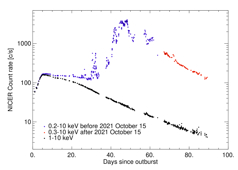
Figure 1: The NICER light curve since optical maximum in the 0.2-10 keV range (black symbols, and red symbols for light curve in the 0.3-10 keV range from 2021 October 15 to avoid contamination from the Sun) and in the 1-10 keV range (blue symbols).

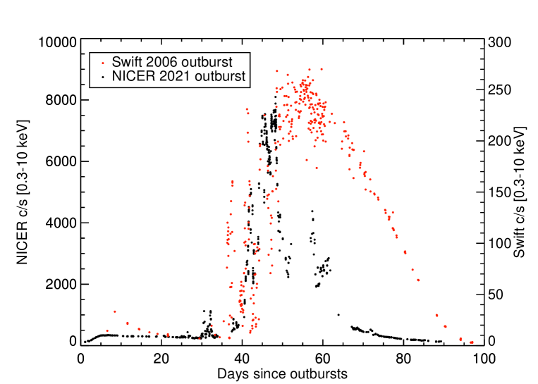
Figure 2: NICER 0.3-10 keV light curve during the 2021 outburst (black dots) compared with the Swift 0.3-10 keV light curve from the previous outburst in 2006 (red dots). The Swift curve was obtained from the online tool at https://www.swift.ac.uk/user_objects/ (Evans et al., 2007). We used PIMMS for the count rate comparison.

During the first 21 days after the outburst, the emission originated in shocked plasma that we attribute to the ejecta and/or ejecta colliding with the red giant wind. Flares of supersoft flux occurred since day 21 post-maximum, and initially they were only short-lasting. The nova became a very luminous, albeit variable, supersoft X-ray source after day 37, with a sharp rise on day 40. The flux of the SSS was overwhelming compared to that of the shocked material, but there was always significant emission also from shocks (the flux up to three orders of magnitude smaller than that of the SSS, but definitely non-negligible). Although there was a similar beginning of the SSS flux in 2006, Fig. 2 shows that in in 2006 there was an extremely luminous flare already on day 35.

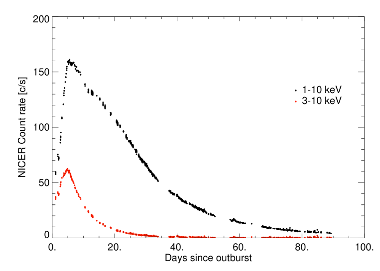
Figure 3: The 1-10 keV NICER light curve is plotted in black and the 3-10 keV light curve in red.

Table 1: Stages of evolution of the outburst as seen in X-rays

X-ray phase	When	Characteristics
NEI shock phase	5 $\leq$ t $\leq$ 11 days	Thermal plasma NOT yet in equilibrium
“Only shocks” phase	day 1 to 21	Thermal plasma emission, L${}_{\rm X,max}=6.8\times 10^{36}$ erg cm-2 s-1
Hot thermal plasma	t $\leq$ 6 days	Initially dominant hot component, kT$\leq$ 40 keV
“Multi-phase” thermal plasma	t $\leq$ 6 days	A second, “cooler” component emerges, with kT$\leq$ 1 keV
First periodic modulation	day 13	Clear modulation with 66.7 s period lasting $\geq$ half hour
Emergence of very luminous soft flux	day 21-25	Additional very “soft” component emerges
		Soft flux possibly only in unresolved emission lines
Soft flares	day 21 to 37	Soft flux increases with sparse, irregular “bursts”
		Soft flux either in emission lines or continuum
Short period modulation	day 26 to 65	$\simeq$ 35 s QPO with decreasing “drift”
Luminous blackbody/atmospheric emission	day 37 to 65	SSS emission of central source (continuum)
Irregular variability	days 40 to 60-65	Changing ionization in absorbing ejecta?
Cooling of central source	days 60-90	Decline to turn-off
Turn-off, end for “sun constraint”	days 70-90	Shocked plasma still measurable

4 Spectral lines and spectral fits: the initial shocks

Fig. 3 illustrates the cooling process of the shocked plasma by comparing the light curves in the 1-10 keV and in the 3-10 keV range. The average spectra of each day during the first week are shown in Fig. 4, while Fig. 5 shows a snapshot of the average spectrum every 4 days for the following 24 days. The panel on the top right in Fig. 4, shows how at the softer energy the flux increased in the first week as new emission lines emerged: Mg XI on the second day, Ne X only the fourth. The plot on the bottom left, illustrates the flux increase between 2.7 keV and 4.7 keV until the sixth day, particularly on the third, followed by cooling only on the 7th day. Cooling is even more evident in the bottom right panel, zooming on the iron feature of the Fe XXV He-like triplet around 6.7 keV. There was a a standstill between the third and fifth day, followed by flux decrease from day 6. The flux in the unresolved Fe XXV helium-like triplet was always much larger than that in the H-like Fe XXVI feature at 6.97 keV. Fig. 5 shows that cooling continued during the whole second week. A complex of lines in the softest range emerged, including unresolved “soft” emission lines, which we attribute mostly to N VI and N VII (NICER’s spectral resolution in the softest range is not sufficient to resolve lines).

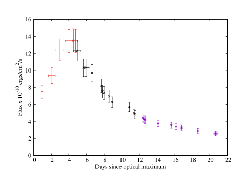
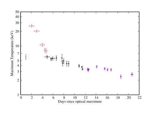
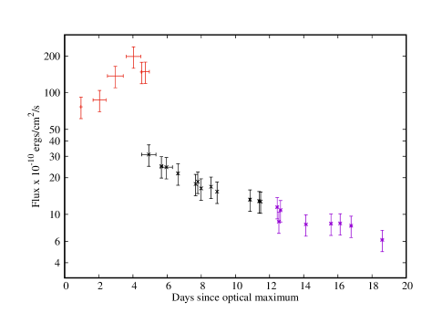
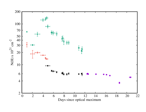
Figure 6: For the first 20 days: in the left upper panel, absorbed flux derived by model fitting, in the left lower panel, absolute flux, in the upper right, plasma temperature of the hotter component (or only component for the red points), in the lower right panel, column density N(H). NEI model fits were used in the first 5.5 days of observations and their parameters are plotted in red. A second component from day 5.5 has a temperature around 0.9 keV in all exposures. The N(H) values in green are the ones of the partially covering absorber (see text for covering fraction) and the 2-component BVAPEC parameters have been plotted in black if there was the partially covering absorber, in purple if this addition was not necessary. The y-axis error bars show the largest of the 2$\sigma$ error in the positive and negative direction, calculated assuming that the other parameters do not vary. The x-axis error bars show the time interval over which the spectrum was integrated. Individual short GTIs were chosen for spectra extraction and fitting when there was significant variability during the day.

Spectral fitting was done by us with the XSPEC tool (Arnaud, 1996), initially with version 12.10 and in the conclusive phase checking the results with version 12.13, after the data were binned with the GRPPHA tool (see Dorman & Arnaud, 2001). While the general evolution of the X-ray spectrum has also been monitored with the Swift XRT and the general trends illustrated in our Fig. 6 were found also by Page et al. (2022), with NICER we obtained a much more detailed picture than with Swift, measuring several emission lines. The NICER monitoring was also denser than the Swift one, with several $\approx$1000 s long GTIs almost every day. Like in the analysis of the Swift XRT spectra (Page et al., 2022), and in that of the high resolution X-ray spectra of the third week (Orio et al., 2022a), we rule out an additional power law model component that could have been produced by non-thermal emission. The unusual strength of the He-like lines in a gas that seems so hot that it should be almost completely ionized, prompted us to explore the possibility of departure from collisional ionization equilibrium, with the VPSHOCK model in XSPEC of parallel shock plasma at constant temperature (initially studied for supernova remnants, see Borkowski et al., 2001). We also explored the addition of a partially covering absorber, that we added to the models to obtain a better fit until day 11. This means that we assumed that one fraction of the emitting surface had additional column density, as may be expected from intrinsic absorption near the source, due to a non-spherically symmetric outflow.

Fig. 6 illustrates the evolution of the absorbing column density N(H) and of the maximum plasma temperature obtained with our spectral fits using XSPEC. The apparent discontinuity in the absolute flux after day 5 is due to switching to the XSPEC BVAPEC model of plasma in collisional ionization equilibrium (CIE) (Brickhouse et al., 2005). The change in the spectrum from NEI to CIE was not abrupt; on the same day around the transition from one model to another, two different models fit almost equally well and this is the case until day 12. However, around day 5.5 the NEI models are no longer necessary, because an equally good result is obtained with two BVAPEC component and a partially covering absorber extended to a fraction that decreased from 60% to about 40%. Starting on day 8, a second soft component appears necessary in both NEI and CIE fits. In the NEI fits, the less hot component turns out to be about 0.3 keV, compared to a value of 0.9-1.0 keV resulting in the CIE case. The hotter component turns out, in fact, to be about 20% hotter in the NEI case, compensating for this difference. The “global” column density and that of the partially covering absorber are both higher in the NEI model than in the CIE one, resulting in a larger absolute flux, up to of few times 10^-8 erg cm^-2 s^-1 and increasing until day 11.

In Table 2 and Fig. 7 we show the parameters of different models fits to the data for a selected GTI of day 7, when also the NEI fit is possible with only a “hot” component. Both fits have the same statistical probability, with a reduced $\chi^{2}\simeq$1.2. The NEI fit, with higher temperature, better predicts the strength of some lines, but we begin to see discrepancy at the softest energy. This discrepancy increased in the fit to the spectra of the following $\simeq$24 hours, when the second, soft component is needed in both the NEI and CIE fits.

Between day 5.5 and day 11 we obtain fits with similar values of $\chi^{2}$/(degrees of freedom) - hereafter reduced $\chi^{2}$ - between 1.0 and 1.4, with both the NEI and CIE model. Guided by the principle of an Occam’s razor, in Fig. 6 we present the main parameters of the BVAPEC fits from day 5.5, because they indicate a decreasing absolute flux with the temperature, in contrast with the result of the VPSHOCK model, which is less intuitive and implies that the absolute luminosity was even above Eddington level during the shock phase. The BVAPEC fits also have fewer free parameters. Moreover, a puzzling issue of the NEI fits is the low value of the electron density and an increasing discrepancy between the value obtained form the ionization time scale and the lower limit obtained from the electron density. All this said, we cannot rule out that the transition to equilibrium occurred only around days 11-12.

It is also interesting that the fraction of the partially covering absorber decreases, and on day 12 it is no longer necessary to obtain a good fit. On day 18, Chandra High Energy Transmission Gratings spectra, in which detailed line ratios were obtained and He-like triplets were resolved, was fitted well with an equilibrium model with two components (Orio et al., 2022a). The same model used for the HETG fits, with almost the same parameters, the NICER spectrum of the GTI closer in time to the Chandra exposure.

While the total flux in the 0.2-12 keV band increased until the end of the 5th day, the maximum plasma temperature peaked already by the third day. However, due to the absorbing column density (complete and partial), the unabsorbed total flux also seems to have increased for the first 4 days (or for even longer assuming a NEI model). We saw in Fig. 4 that the flux in the prominent Fe XXV decreased in intensity only after the fifth day (transition from cyan to pink curve in the figure), consistently with the maximum temperature returned by the fits. In the second and third week, the plasma was constantly cooling, with a rapid “softening” of the spectrum (Fig. 5).

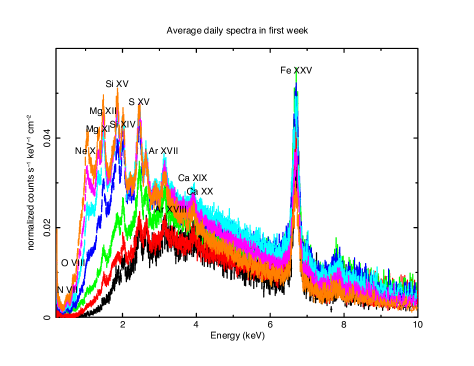
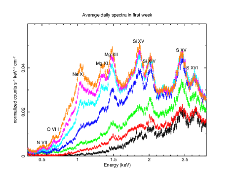
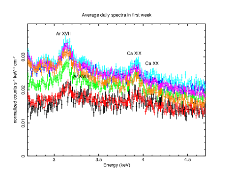
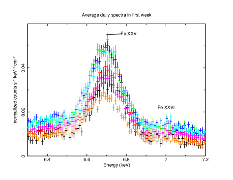
Figure 4: The average count-rate spectra observed with NICER from day 1 to 7.5. The dates are 2021 August 10 (black, observation 4202300101), August 11 (red, obs. 4202300102), August 12 (green, obs. 4202300103), August 13 (dark blue, obs. 4202300104), August 14 (cyan, obs. 4202300105), August 15 (pink, obs. 4202300106) and August 16 (orange, obs. 4202300107). The prominent emission lines are marked.

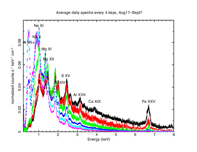
Figure 5: The average daily spectra observed with NICER in the period between days 8 and 29, plotted every 4 days. The colors sequence in order of date is black (2021 August 17), red (August 21), blue (August 25), green (August 29), cyan (September 3), pink (September 7).

In Fig. 7 we show the ratio of the emissivities of Si XIII/Si XIV and S XV/S XVI as a function of temperature derived from the ATOMDB database in collisional ionization equilibrium (CIE) and Non Equilibrium Ionization (NEI) regimes. In the case of non-equilibrium plasma (NEI), we assumed $\tau=10^{11}$ s $\times$ cm^-3 (a value closed to those obtained in the fits, see discussion below). These ratios are more sensitive to temperature in the CIE regime than in the NEI regime. The measurement show that the values returned by fitting Gaussian profiles and subtracting an “ad hoc” continuum for different maximum temperatures obtained with the fits described below, seem to be always above the NEI values for Si and for temperatures higher than about 5 keV also for S.

While the departures from collisional ionization equilibrium explain the unusual line ratios, more than one plasma component at different temperature can also interplay to explain this phenomenon. From the middle of the sixth day, the temperature is in a range such that the spectrum can be fitted in both ways. From day 12, we ruled out that the NEI model is adequate, and we conclude that most likely, equilibrium had been reached.

The abundances of elements from carbon to iron were allowed to vary in these fits, but to avoid too many free parameters, we assumed that they abundances were the same in the two plasma components. Although in both VPSHOCK and BVAPEC, we allowed the abundances to deviate from solar, the results are within rather large, (20-30%) statistical errors. Only nitrogen results constantly enhanced, while iron turns out to be depleted (see Orio et al., 2022a). The abundances of elements of atomic number between carbon and calcium, except nitrogen and iron, in most fits are somewhat enhanced above solar, depending on each element.

There is a caveat in the NEI fits. The upper limit to the ionization time scale, a parameter of the fit, is consistently only a few times 10¹¹ s cm^-3. This implies unusually low electron density, varying from a few 10⁵ to a few 10⁶ cm^-3 for the medium in which the hotter component is produced. Table 2 reports also an lower limit, close to 10⁷ cm^-3, that we would obtain instead from the emission measure assuming that the medium has filled a spherical volume expanding at $\simeq$7550 km s^-1 (from the radio Munari et al., 2022) and that flux has origin in the whole volume. This is consistent with the electron density inferred from the material emitting the flux at radio wavelengths (Munari et al., 2022). This limit is obtained with the highest velocity measured during the outburst, but with the lower velocity of $\simeq$2800 km s^-1 inferred from the optical H$\alpha$ line at the beginning of the outburst (Fajrin et al., 2021), the resulting lower limit on the electron density would be even higher by a factor of 20, so clearly there is a tension between the two values derived from the emission measure and from the ionization time scale.

On day 18 the X-ray flux of RS Oph seemed to originate in very dense clumps of matter, with much higher electron density than the average Orio et al. (2022a), like in V959 Mon, (Peretz et al., 2016) and V3890 Sgr, (Orio et al., 2020). The line ratios diagnostics in the X-ray high resolution spectrum RS Oph on day 18 reveal that the emission originated in clumps of material with electron density possibly as high 10¹² cm^-3 (Orio et al., 2022a). Typical values of the electron density in the nova ejecta in the first days have been estimated to be even close to 10¹¹ cm^-3 both in X-rays (e.g. the recent nova V1674 Her, Sokolovsky et al., 2023) and in optical spectra (e.g. Neff et al., 1978, who found a value of 7.4 $\times 10^{-11}$ cm^-3 for V1500 Cyg). Other published values from optical lines in novae span orders of magnitudes, but were mostly obtained at later post-outburst epochs, in the nebular phase. The electron density distribution was estimated between 10⁵ cm^-3 and $\times 10^{7}$ cm^-3 for the symbiotic nova V 407 Cyg (Shore et al., 2012b); it was still between 10⁶ cm^-3 and 4 $\times 10^{7}$ cm^-3 on day 186 of the outburst of V5668 Sgr (Shore et al., 2018), and it was a few times $10^{7}$ cm^-3 about a month after the outburst for the recurrent nova T Pyx (Shore et al., 2012a). For the latter, we also know it was decreasing on time as t^-3, so it must have been significantly higher in the early days. Thus the NEI fits parameters, taken at face value, imply that the initial shocks producing X-ray flux occur not only in a much lower density medium than the thermal plasma we measured at later dates, but also quite lower than estimated in most other novae.

Another intriguing issue is the very high absolute luminosity: in the BVAPEC model it is large, reaching a few times 10³⁷ erg s^-1, but it is predicted to be even super-Eddington in the NEI model. When we are able to fit the spectra with equilibrium models and without adding a partially covering absorber, namely around day 12, the resulting unabsorbed flux is much smaller, but it still exceeds 10³⁶ erg s^-1 for at least another week. The same order of magnitude of absolute flux is extrapolated from the fits’ parameters of Page et al. (2022, see Table 1 on line.)

We note that from day 12 our model is essentially the same as the one in Page et al. (2022), with corresponding temperatures of the two plasma components, but we obtain the fit with only 5.95 $\times$ 10²¹ cm^-2 already on day 12, less than half the value in Page et al. (2022) for the same day. Because NICER is calibrated from 0.2 keV, the data presented here are more sensitive to the absorption and we suggest that the lower in column density is real, although the decrease may have been less sharp and sudden than what is apparent in the plot. We note that the BVAPEC model used by us differs from the APEC model used by Page et al. (2022) for Swift, because it includes abundances, line width and velocity as parameters. Although the fits were not very sensitive to the blue shift velocity, a small broadening velocity of $\simeq$500-800 km s^-1, consistent with the precise measurements with the X-ray gratings (see Orio et al., 2022a), generally improved the fits. However, the variable abundances are probably the main cause of the difference between our fits and the Swift ones of Page et al. (2022).

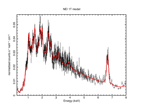
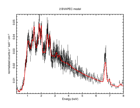
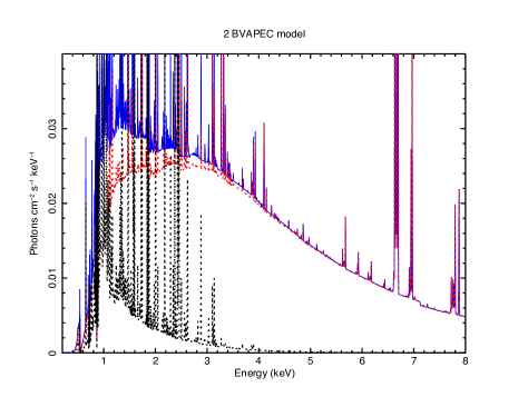
Figure 7: For the 4th GTI of day 7, August 16, the top panels show the fits with a plasma that is not in equilibrium, and with two plasma components at different temperature and in collisional ionization equilibrium, respectively on the left and the right. The bottom panels show the corresponding models before convolution with the instrument response. The fit parameters are in Table 2. The fit on the right shows the “hot” component in red, the “cool” one in black, and the result is shown in blue.

5 The soft flares

Like in 2006, the initial rise of the SSS was marked by short flares of extremely soft flux. On August 28 (day 18), a new phenomenon started. During a very brief GTI that lasted for only 45 s and was interrupted for technical reasons, there was a large increase in flux below 0.6 keV. The quality of the data was checked with more than one method, and the large brightening in this short GTI appears to be due to the source, not to space weather or background. On August 30 (day 21), as Fig. 9 shows, at the beginning of the exposure, the count rate in the 0.2-0.6 keV range was much higher than the average count rate measured two days earlier, but decreased again on that day. An XMM-Newton exposure was started $\simeq$ 3 hours after the end of the NICER observations: the XMM-Newton EPIC pn light curve, shown by Orio et al. (2022a), continued to show a steady decrease. The lightcurve and the spectra at maximum and minimum on day 21 are plotted in the left panels of Fig. 9. The soft energy excess can be fitted either like in Page et al. (2022), by adding a third blackbody component, or instead with an additional BVAPEC component at lower temperature. At energy $>$0.5 keV the spectrum was unchanged and only the softest portion appeared to flare. The grating spectra analyzed by Orio et al. (2021a) indicate that this initial soft excess was more “structured” and complex than a blackbody, and was most likely due to new emission lines appearing in the soft range.

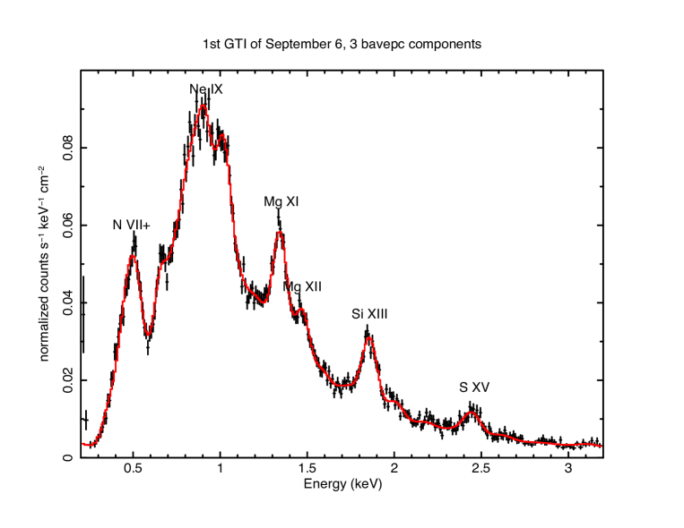
Figure 10: The spectrum of the first GTI of day 28 (2021 September 6), during a “quiet” day after the flare described above. The red line traces the fit with Model 3 of Table 3 (in red).

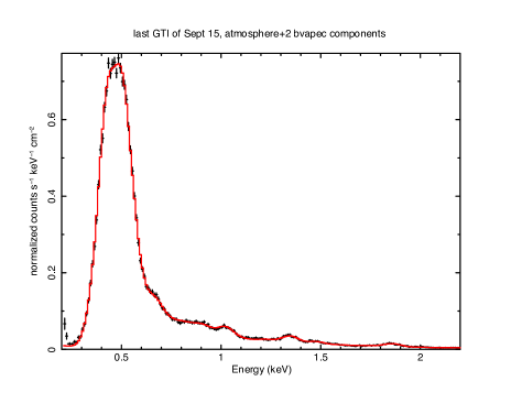
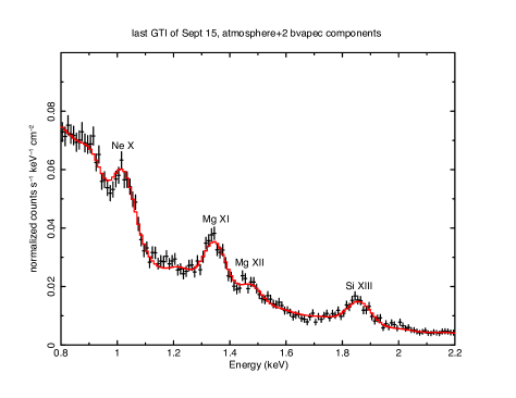
Figure 11: Two portions of the spectrum of a flare on day 37 (2021 September 15). The red line traces the fit with Model 1 in Table 4.

Another, large soft flare was observed the beginning of an exposure on September 5 (day 27), as shown in the plots on the right in Fig. 9. The spectrum observed after the flare on the following day is shown in Fig. 10 and the possible models that fit it are in Table 3. In the following days, there were several more soft flares lasting for up to a few hours. Both during and after the flares, the spectra can be modeled with an equally good fit either by adding to the two CIE plasma components (BVAPEC model) a blackbody affected by the same column density as the thermal plasma and a temperature of 80-90 eV, like in Page et al. (2022), or a third low-temperature BVAPEC thermal component like in Orio et al. (2022a), initially with temperature around 200 eV and cooling to $\simeq$90 eV in the following 10 days. Most fits required an additional absorbing column density for this soft component. Figs. 11 shows that the soft excess on day 37 peaked around 0.5 keV, which corresponds to the N VII H-like line, however adding a third plasma component at low temperature with elevated nitrogen does not fit the spectrum. In fact, the apparent line is too broad to be a single emission line.

The high resolution spectra obtained with XMM-Newton on day 21 (2021 August 30) were taken during the decline, but they do indicate that, at least in this early phase, the larger soft flux was in several emission lines that later seemed to fade or disappear (see Fig. 7 of that article). NICER cannot resolve well emission lines at energy $\leq$0.7 keV keV.

We fitted also the spectra of this phase with enhanced abundances with respect to solar, mostly 2-7 times for all elements except for nitrogen (overabundant by up to a factor of 70) and depleted iron, but the abundances values have large uncertainty. The iron abundance turns out to be consistently depleted by a factor of a few. The nitrogen overabundance indicates mixing with ashes of the CNO burning, but given errors up to 50% in the determination of the abundances of this element, we cannot draw a firm conclusions. Orio et al. (2022a), using high resolution X-ray grating spectra, derived enhanced abundance of nitrogen on day 30 and depleted iron on days 18 and 21. We note that enhanced abundances of the other elements are somewhat unexpected, because the ejecta are being diluted by the interaction with the red giant wind.

We give examples of fits’ parameters in Tables 3 and 4; some of the model fits are also plotted in in Fig. 9, 10 and 11. Table 3 presents as many as three different fits for an out-of-flare GTI, one with a blackbody, the second and the third with different N(H) for one of the components. Table 4 show the parameters that fit the last flare before a more permanent, steep rise on day 37. If we assume additional absorption for the coolest component, its temperature is higher, and the resulting absolute flux is as large as 6 $\times 10^{-9}$ erg s^-1 cm^-2. The absorbed flux in the same exposure was a little over 1.7 $\times 10^{-10}$ erg s^-1 cm^-2. The parameters can be compared with Page et al. (2022). The NICER spectra, with a lower energy range (calibrated and reliable from 0.2 keV instead of 0.3 keV as the Swift XRT) constrain N(H) to be significantly lower than the value obtained by Page et al. (2022) in the same period.

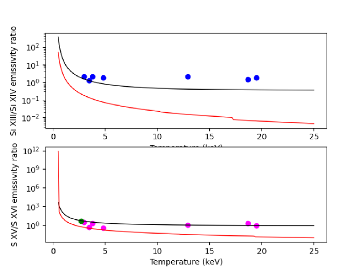
Figure 8: Predicted flux line ratios of Si XIII/Si XIV and S XV/S XVI (including all the merged lines for the He-like triplet) for a single temperature plasma region, under the assumption of collisional ionization equilibrium (CIE, in red) and assuming non-equilibrium (NEI, in black, like in the “VPSHOCK” XSPEC model, with ionization time scale parameter 10¹¹ cm $\times$ s). The dots indicate actual measurements in correlation with the maximum temperature of an acceptable fit to NICER spectra; the green dot in the lower panel shows a measurement with a resolved triplet, with the Chandra HETG grating from Orio et al. (2022a). In that paper a very good fit to the overall spectrum was obtained assuming two regions at different temperature and in CIE, instead of a single region in NEI.

Until the large increase on day 37 (September 16) all fits result in $\chi^{2}$/d.o.f. in the 1.1-1.5 range, either using either a “central source” (blackbody or atmosphere) and two thermal components, (like in Page et al. (2022)) or using three BVAPEC components. For most GTIs, however, the spectra are fitted by assuming at least two different values of the absorbing column densities N(H), and as shown in Table 3, different combinations of temperature and (NH) can give an equally good fit. Table 4 compares fits for the spectrum of a flare of 2021 September 15, day 36. We notice that, around day 33 (September 11), substituting the blackbody with an atmospheric model from Rauch et al. (2010) gives a much better fit, but only if we add also another very soft thermal plasma component with a temperature of 80-90 eV. Thus it is likely that the soft flux at this stage actual due to both emission in a thermal plasma and to the appearance of the SSS continuum. The fits with the atmospheric models indicate that the WD would initially have an effective temperature of 450,000 K, with a bolometric luminosity around 7 $\times 10^{37}$ erg s^-1 (see Table 4). When the source is not flaring, the very soft blackbody or atmospheric component is still necessary in the fit, but and it contributes to the observed flux by only a few %. During the flares, already after day 30 this component contributes by more than 60% to the unabsorbed flux.

Table 2: Parameters of the fit of the fourth GTI of day 7 (2021 August 16) with two different models: a VPSHOCK model in XSPEC of non-equilibrium thermal plasma (Model 1), and two two BVAPEC plasma components (Model 2). This is the last day in which a fit with one temperature can be obtained; a second component then becomes necessary also in the NEI assumption. NEI models no longer fit from day 12. If there was not a large difference in the 2$\sigma$ statistical error in the positive and negative direction, we only report the largest one; the errors are calculated assuming that the other parameters are fixed. n*_e is the value of the electron density resulting from the ionization time scale, while below it we report a lower limit derived from the emission measure.

	Model 1	Model 2
$\chi^{2}$/d.o.f.	1.2	1.2
N(H) $\times 10^{21}$ cm-2	10.7$\pm$0.9	6.8$\pm$0.3
N(H)${}_{\rm part.}\times 10^{21}$ cm-2	47.92$\pm$18.9	58.3$\pm$5.9
Cov. Fract.	0.49$\pm$0.08	0.71$\pm$0.03
T1 (keV)	7.24$\pm$0.54	5.52$\pm$0.51
T2 (keV)	—-	1.04$\pm$0.03
N/N⊙	45${}^{+61}_{-15}$	36${}^{+30}_{-19}$
Fe/Fe⊙	0.6$\pm$0.2	0.4$\pm$0.1
$\tau_{\rm max}$ (s $\times$ cm-3)	3.42$\pm 0.85\times 10^{11}$	–
EM1 cm-3	5.71 $\times 10^{58}$	3.19 $\times 10^{58}$
EM2 cm-3	–	5.96 $\times 10^{57}$
n*e cm-3	6.1 $\times 10^{5}$	–
ne cm-3	$\geq 1.2\times 10^{6}$	$\geq 9.7\times 10^{6}$
F${}_{\rm x,abs}\times 10^{-10}$ erg cm-2 s-1	10.12	9.73
F${}_{\rm x,unabs}\times 10^{-10}$ erg cm-2 s-1	76.12	22.22

Table 3: Parameters of the fit of the first GTI of day 27 (September 6), with three different composite models: a blackbody and two BVAPEC plasma components (Model 1), or three BVAPEC thermal plasma components (Model 2 and 3). In Model 3 all components are affected by the same column density, while in Model 2 the coolest and hottest component are absorbed by N(H)_1,2,3+N(H)_1,3. The flux of the single components is numbered in order of rising temperature. If there was not a large difference in the 2$\sigma$ statistical error in the positive and negative direction, we only report the largest one; the errors are calculated assuming that the other parameters are fixed. The electron density with a star is obtained from the maximum ionization time scale, while the lower limit on the electron density is obtained from the emission measure assuming an expansion velocity of 7550 km s^-1..

	Model 1	Model 2	Model 3
$\chi^{2}$/d.o.f.	1.5	1.3	1.3
N(H)1,2,3 $\times 10^{21}$ cm-2	3.4$\pm$0.2	2.6$\pm$0.1	3.1$\pm$0.3
N(H)1,3 $\times 10^{21}$ cm-2	0	7.9$\pm$0.7	5.7$\pm$0.2
Tbb (eV)	45.2$\pm$0.6	–	–
T1 (eV)	–	290$\pm$80	90$\pm$18
T2 (keV)	0.66$\pm$0.02	0.73$\pm$0.08	0.80$\pm$0.03
T3 (keV)	2.27$\pm$0.30	1.85$\pm$0.30	4.89$\pm$2.30
F(tot) $\times 10^{-10}$ erg cm-2 s-1	1.74$\pm$0.91	1.73$\pm$0.32	1.77$\pm$0.14
F(tot,unabs) $\times 10^{-9}$ erg cm-2 s-1	1.41$\pm$0.59	6.25$\pm$0.77	3.32$\pm$1.17
Fbb $\times 10^{-11}$ erg cm-2 s-1	0.30$\pm$0.02	–	–
F(bb,unabs) $\times 10^{-10}$ erg cm-2 s-1	9.17$\pm$0.73	–	–
F(1) $\times 10^{-11}$ erg cm-2 s-1	–	2.95$\pm$1.48	0.87$\pm$0.80
F(1,un) $\times 10^{-9}$ erg cm-2 s-1	–	5.87$\pm$2.90	2.84$\pm$2.70
F(2) $\times 10^{-11}$ erg cm-2 s-1	5.53$\pm$0.45	9.53$\pm$3.83	13.85$\pm$10.00
F(2,un) $\times 10^{-10}$ erg cm-2 s-1	1.00$\pm$0.08	2.59$\pm$1.04	4.35$\pm$0.35
F(3) $\times 10^{-10}$ erg cm-2 s-1	1.16$\pm$0.12	0.48$\pm$0.24	0.32$\pm$0.15
F(3, un) $\times 10^{-10}$ erg cm-2 s-1	3.89$\pm$0.39	1.22$\pm$0.28	0.43$\pm$0.20

Table 4:

Parameters of the fits to the last, and highest GTIs of day 36 (2021 September 15), with two different composite models: a WD atmosphere and two BVAPEC plasma components (Model 1), or three BVAPEC thermal plasma components (Model 2). The flux of the single components is numbered in order of rising temperature. The second component, of intermediate temperature, has an added column density N(H)₂. The errors are calculated and presented as in Table 2.

	Model 1	Model 2
$\chi^{2}$/d.o.f.	1.1	1.1
N(H)1,2,3 $\times 10^{21}$ cm-2	4.92$\pm$0.04	1.96$\pm$0.10
N(H)2 $\times 10^{21}$ cm-2	–	2.26${}^{+0.70}_{2.20}$
Tatm (K)	450,000$\pm$5,000	–
T1 (eV)	90.5$\pm$89.0	93.1$\pm$5.9
T2 (keV)	–	0.57$\pm$0.04
T3 (keV)	0.62$\pm$0.02	1.38${}^{+0.68}_{-0.21}$
F(tot) $\times 10^{-10}$ erg cm-2 s-1	2.15	2.17
F(tot,unabs) $\times 10^{-8}$ erg cm-2 s-1	14.7${}^{14.0}_{-4.0}$	1.48${}^{+1.45}_{-0.52}$
Fatm $\times 10^{-11}$ erg cm-2 s-1	1.10$\pm$0.60	–
F(atm,unabs) $\times 10^{-7}$ erg cm-2 s-1	1.08$\pm$0.60	–
F(1) $\times 10^{-10}$ erg cm-2 s-1	1.27${}^{+0.42}_{-1.20}$	0.77$\pm$0.09
F(1,un) $\times 10^{-9}$ erg cm-2 s-1	38.3${}^{+35.0}_{-10.7}$	0.48$\pm$0.06
F(2) $\times 10^{-11}$ erg cm-2 s-1	-	8.85${}_{-3.74}^{+23.8}$
F(2, un) $\times 10^{-10}$ erg cm-2 s-1	-	3.93${}_{-1.66}^{+3.7}$
F(3) $\times 10^{-10}$ erg cm-2 s-1	0.77$\pm$0.17	0.53$\pm$0.11
F(3, un) $\times 10^{-10}$ erg cm-2 s-1	379$\pm$65	1.23$\pm$0.02

In the 2006 outburst, flaring was observed on day 27 post-maximum during a long exposure with XMM-Newton in the supersoft region, and the high resolution spectrum showed that it was due to the appearance of prominent emission lines (Nelson et al., 2008). Also in 2021, it is likely that even for several days, the first manifestation of the SSS presence is in an emission line spectrum, due to material that is either photoionized or shock-ionized quite close the WD. However, due to the degeneracy in the combination of column density and temperature in the fit, we cannot exactly determine when the WD becomes visible. It is important to notice that the flares do not appear to be due to increasing blackbody/atmospheric temperature, neither to decreasing column density; actually the fits improve with even increased column density in the flares’ spectra, as if new material has been emitted in parallel to the emergence of the SSS, and is contributing to some more intrinsic absorption.

6 The “stormy” luminous supersoft X-ray phase

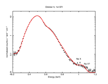
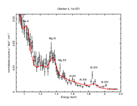
Figure 13: The spectrum of RS Oph observed with NICER in the first $\simeq$1000 s long GTI of day 57 (2021 October 5), fitted with a blackbody at a temperature of 37 eV, absorbing column density N(H)=4.3 10²¹ cm^-2 with non-solar abundances of C and O (C/C_⊙=4.9, N/N_⊙=2.5), two components of BVAPEC thermal plasma at 81 eV and 462 eV. The flux is 1.74 $\times 10^{-9}$ erg s^-1, of which the BVAPEC thermal plasma contributes only less than 2%. The total unabsorbed luminosity would be about 2 $\times 10^{40}$ erg s^-1 (a blackbody overestimates the luminosity, see text for the discussion).

The supersoft X-ray phase was quite different from the 2006 outburst. It was less luminous, shorter lived and with more episodes of irregular, large variability, that occurred even within hours, as shown in Fig. 12. Fig. 13 shows the spectrum at peak. The less soft portion of the spectrum still shows the presence of the shocked thermal plasma, that by this time had cooled to temperatures below 0.5 keV.

One challenge posed by the luminous supersoft X-ray spectra of novae in general, and specifically of RS Oph in 2006 and 2021, is that most high resolution X-ray spectra obtained with the Chandra and XMM-Newton gratings show blue-shifted absorption lines (Rauch et al., 2010; Ness et al., 2011; Orio et al., 2021b; Ness et al., 2022a, e.g.), indicating that we are not simply observing an atmosphere at rest. The blue-shift can be large, corresponding to even 2000 km s^-1 for many features of some novae; this is in contrast with a key assumption in the models, that by the time the central WD becomes observable, mass loss has ceased (Kato & Hachisu, 2020, e.g.). Reasonable fits to the SSS spectra have been obtained in the following semi-empirical ways:

$\bullet$ We can assume that we observe a small shell of material near the WD atmosphere that has recently been detached and is expanding, thus modeling the spectrum with a photoionization code for X-ray astronomy, assuming that the photoionizing source is a blackbody, whose temperature is a fit parameter. This has been done with varying results (Ness et al., 2011; Orio et al., 2021b; Ness et al., 2022b; Milla & Paerels, 2023). Sometimes, many shells have to be included to fit the spectra, introducing many variable parameters (Ness et al., 2011, see), so the parameterization becomes more uncertain. This approach relies entirely on modeling the absorption features and edges, but the features are not resolved in this range with a broad band spectrum like NICER’s.

$\bullet$ van Rossum (2012) computed a model inspired by the physics of the winds of massive stars for nova V4743 Sgr and made a grid of models publicly available. In this model the blue-shift of the lines is parameterized by mass outflow rate and effective effective temperature. The model predicts how the the line profiles change with blue-shift (wind velocity), but it does not give satisfactory results for other novae (Orio et al., 2018). We cannot not measure absorption line profiles with NICER, so we did not try this model.

$\bullet$ A third, common approach is an atmospheric model (Rauch et al., 2010), assuming in first approximation that all the absorption features keep the basic profile of the atmosphere “at rest”, even if they are generated in a wind. The features are then assumed to be blue-shifted with the velocity as a free parameter. In other words, one assumes that the photoionized source is the WD and that the structure of the absorption spectrum does not change in material that is being detached, but is very still close to the WD. This approach often yields a good fit, including the departure from a blackbody continuum that is always observed. It has been used in the literature to fit the broad-band X–ray spectra of novae, using the shape of the continuum and sometimes adding absorption edges. Osborne et al. (2011); Page et al. (2022) for instance experimented with it fitting RS Oph XRT’s spectra of 2006 and 2021. Nelson et al. (2008) fitted the high resolution 2006 spectra of RS Oph with a peak temperature of about 800,000 K; however, not all spectral features were explained, also because there is a limited available grid of abundances, that may not be suitable for RS Oph or other novae.

$\bullet$ For broad band spectra, another possibility is to assume a blackbody and include absorption edges that change or “cut” the shape of the continuum. This has been done by Osborne et al. (2011); Page et al. (2022) for RS Oph. Page et al. (2022) found that the Swift XRT spectra of 2006 have much deeper absorption edges than the 2021 ones. They fitted the SSS phase adding two components of thermal plasma to a blackbody, modified by “ad hoc” absorption edges, similar to those of a WD atmosphere. However, also in the luminous SSS phase the NICER spectra give a more complex picture than the Swift XRT ones. One reason is that, as an imaging telescope, Swift XRT yields data that are strongly affected by pile-up for such a luminous and soft source. The spectra examined in (Page et al., 2022) are obtained by cutting off the central region of the point spread function, to avoid the effects of pile-up. We did not find spectra of exactly overlapping GTIs for Swift XRT and NICER, but if we consider a spectrum taken on 2021 October 5 approximately 3 hours after and before exposures by NICER, we observe in Fig. 14 how the spectrum extracted from the “non-piled up annulus” is much “flatter” than the the NICER ones, so if one simply assumes that the flux has been reduced by a constant factor, the translation makes the wings of the spectral distribution excessively broad. Thus, a straightforward spectral fit tends to converge towards a higher value of the column density N(H) and a higher blackbody (or atmospheric) temperature than the value we obtained fitting the NICER spectrum. The inclusion of absorption edges corrects this effect, but it is empirical and may not necessarily have physical meaning. Correcting the pile-up corrected Swift spectrum assuming that the flux is reduced by an energy-dependent factor may be a complex task.

Given all the above considerations, we limited our attempts to fit the NICER spectra to a blackbody and to the atmospheric model (Rauch et al., 2010), with the addition of a CIE (BVAPEC) model thermal plasma. This thermal plasma has flux at least 3 orders of magnitude smaller than the central source, but it modifies the SSS continuum. In fact, in the portion of the spectrum in which the continuum is low, emission lines are still prominent, and resolved above 1 keV (see panel on the right in Fig. 14). We experimented with several models in the public grid of the Tübingen non-local-thermodynamic-equilibrium atmosphere TMAP(see http://astro.uni-tuebingen.de/#rauch/TMAP/TMAP.html and Rauch (2003); Rauch et al. (2010)). Tübingen grid 003 model was found to be a reasonable fit to the 2006 high resolution spectra (Nelson et al., 2008). Similarly, (Osborne et al., 2011) found that this particular model reproduced the continuum for several Swift XRT broad band spectra of 2006. However, we did not obtain a rigorous fit for the NICER spectra of 2021 with this model, neither with the others in the grid. One reason is the extreme difficulty in making the fit converge in XSPEC with two components at such different flux magnitude. Like Page et al. (2022) we found that including the thermal plasma (with much lower flux than the “central source”) is essential also where it overlaps with the strong SSS continuum, because it modifies it.

At peak luminosity the best of the fits with this model to several spectra around the peak (second half of September 2022) returns an effective temperature of about 750,000 K, much higher than obtained for day 37 in Table 4, but slightly lower than obtained by fitting the high resolution spectra in 2006 (Nelson et al., 2008). We obtained column density N(H)=4.7 $\times$ 10²¹ cm^-2 and bolometric luminosity 2 $\times 10^{38}$ erg s^-1. At least one plasma component at 217 eV is necessary to improve the fit; a second thermal component around 80 eV improves the fit even more.

Ness et al. (2022a) find that an absorbing medium with varying ionization states can explain the SSS irregular variability. For an XSPEC global fit we did not have a model with varying ionization states, but the TBVARABS model allows to test instead varying the abundances of the absorbing medium. If there is circumstellar absorption of the red giant wind and wind mixed with ejecta, it is reasonable to expect non-solar abundances. The fit with TBVARABS, a blackbody and additional thermal plasma is closer to the observed spectrum and is shown in Fig. 14. In TBVARABS we let the abundances of carbon and oxygen vary and found that we much improve the fit if they are enhanced (the first 4.9 times solar, the second 2.5 times solar, and slightly depleted oxygen (0.82 times solar). The resulting column density N(H) is still higher than for the same day in Page et al. (2022)’s fits, 4.3 $\times 10^{21}$ cm^-2, and the temperatures of the two thermal components are 81 eV and 462 eV, respectively. The blackbody has a temperature of 36.6 eV (only $\simeq$425,000 K), but its bolometric luminosity would have to be much over Eddington level, namely about 2 $\times 10^{40}$ erg s^-1 (a blackbody is known to overestimate the luminosity, e.g. Heise et al., 1994). We do not consider this a realistic fit, but it is an experiment to guide a future analysis in which the XMM-Newton RGS grating spectra (see Ness et al., 2022a) will be the starting point. A rigorous model for the SSS spectrum should first rely on the high resolution spectra, and we leave it for future work. We focus in the following sections on other results we obtained with NICER alone for the SSS phase, its duration and variability.

7 The aperiodic large-amplitude variability

An interesting characteristic of the SSS phase is the large irregular variability (even by a factor of 100%, see Fig. 12) over time scales of hours and days. Even if our fits are only qualitative, we notice that we cannot fit the spectra taken in exposures with high count rate by simply increasing temperature or emission measure, or decreasing column density N(H), used for the fit to low count rate spectra. The NICER data are not compatible with changes in the emitting region size or in the temperature; our qualitative fits with atmospheric models to the spectra of days 40-67 always converge towards T${}_{\rm eff}\simeq$750,000 K, no matter what the count rate is. However, given that our model fits for this phase are still qualitative and not rigorous, we refer here to the discussion of the high resolution X-ray spectra of RS Oph by Ness et al. (2022a), who compared a high resolution XMM-Newton RGS spectrum of RS Oph obtained in 2021, with those of 2006 at different times after the outburst. They discussed three different possibile scenarios:

1. The spectrum during the SSS phase has variable flux, either because of an “eclipsing”, opaque intervening body, or because the WD photospheric radius changes at constant temperature,

2. The central source has varying temperature.

3. The absorption varies on short time scales along the line of sight. Given that varying the column density N(H) does not explain the variability, Ness et al. (2022a) explored the effect of changing ionization stages in the ejecta and in the pre-existing wind.

The last scenario, according to Ness et al. (2022a), is the correct one. In fact, these authors’ physical model of multi-ionization photoelectric absorption does explains the observed variability, while they can fit the high resolution spectra with a central source of constant temperature and flux. This is consistent either with a turbulent, clumpy outflow in which different clumps may have different ionization stages, or perhaps it may be explained by varying conditions in the red giant wind.

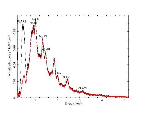
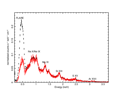
Figure 9: Top: the light curves observed over few hours on day 21 (2021 August 30; left) and day 27 (2021 September 5; right). On day 21, new observations were resumed with XMM-Newton after about 3 hours. The light curve during that exposure shows a continuing decline in flux for the whole day (Orio et al., 2022a). The $\simeq$ 35 s QPO on day 27 was very pronounced during this day. The bottom panels compare spectra during high and low count rate intervals. On the left the spectrum measured on August 30 during the initial GTIs with higher count rate (black, first 130 minutes) compared with that of the last GITs with lower count rate on day 21 (red, last $\simeq$360 minutes) and on the right, the spectrum of the third GTI of day 27 (in black, it lasted for about 400 s) and that of the GTI before the last (in red).

Figure 12: The light curve (0.2-1 keV range, non-background subtracted) for the days of largest supersoft luminosity, between days 44 and 50, and in more detail for 2021 September 18-19 (day 46 of the outburst.

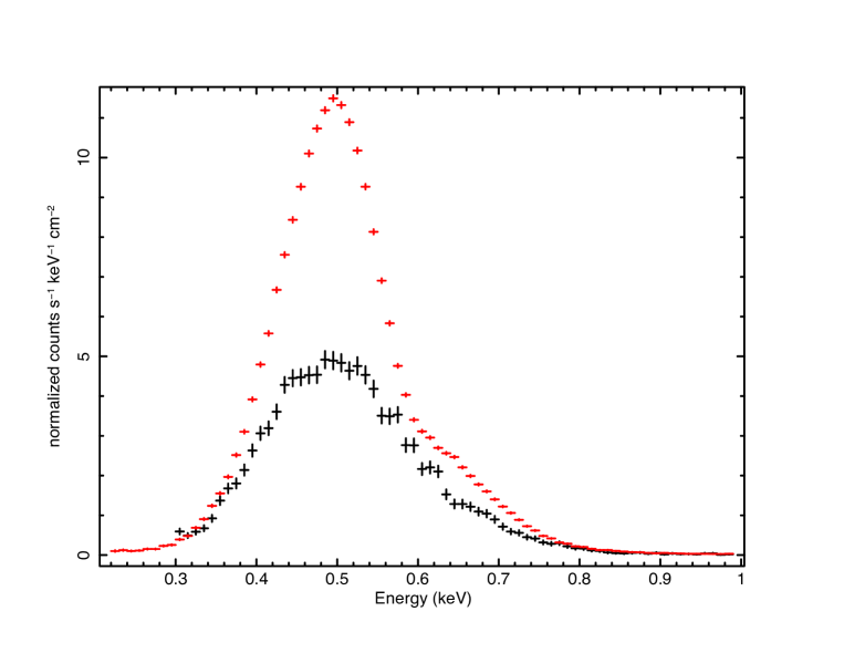
Figure 14: Comparison between the RS Oph spectra below 1 keV obtained on day 57 (2021 October 5) with NICER at 1:37:27 (red) and and the pile-up corrected Swift XRT spectrum of the same day during a 1 ks GTI starting at 4:37:22 (in black), extracted from an annulus around the center of the PSF with the https://www.swift.ac.uk/user_objects/ webtool.

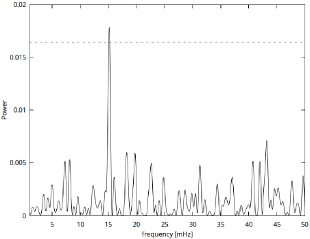
Figure 15: Lomb-Scargle periodogram of the light curve of the 7th GTI of observation 4202300113, 2021 August 22 (day 13). The dashed line shows the 99.99% confidence level.

Figure 16: Two examples illustrating how the modulation with the $\simeq$35 s period is evident even visually. On the left, a portion of the RS Oph NICER lightcurve on 2021/9/18 (day 40) and on the right, a portion of the NICER lightcurve on 2021/9/19 (day 41), both measured in the 0.2-0.6 keV range with 1 s bins.

We also investigated another possibility: that dust may have caused the variability and contributed to the observed X-ray spectrum. RS Oph is not known to have ever formed a significant amount of dusti in previous oitbursts, but there was evidence of dust 2 days after the 2021 optical maximum (Y. Nikolov, private communication). In any case, with such a large supersoft luminosity, even a small amount of dust may affect the X-ray light curve and spectrum. The variability time scale is hours, and the flux amplitude variation is very large, up to 100%. We refer to work done a few years ago by Corrales et al. (2016); Smith et al. (2016); Heinz et al. (2016). Dust scattering may cause variability, because the scattered X-rays traverse a longer path than the X-rays directly received from the source, creating an echo of the X-ray flux of the source. However, amplitude variations of order 100% are not caused by interstellar dust scattering (i.e., scattering from dust not intrinsic to the source), since scattering cross sections are generally very small and the scattered component will emit little flux compared to the flux from the source itself, given the column density towards the source. Dust scattering on time scales of hours for reasonable scattering angles of order $\theta_{\rm sc}\lesssim 300\arcsec$ (above which the scattering cross section at soft energies drops precipitously, see Draine, 2003) would imply that the dust is at distance of several hundred parsecs or more, given the relation between distance $d$ from source to dust and time delay $\Delta t$:

$$d\approx\frac{c\Delta t\cos{\theta_{\rm sc}}}{1-\cos{\theta_{\rm sc}}}$$ (1)

In addition, by virtue of being an echo, if the source is variable, dust scattering by intervening static clouds cannot produce variability on time scales shorter than the intrinsic source variability.

The observed variability time scale can be created if the scatterer itself is moving rapidly enough, relative to the line of sight, for the scattering angle to change by more than $\sim 300\arcsec$. In this case, the variability does not arise from a dust scattering echo but from the dynamically changing scattering geometry. In this scenario, dust clouds in the outflow or in the circumstellar environment of RS Oph would need to move rapidly enough, be numerous enough, and each scatter enough of the source flux to create not only the observed time scale, but also the repeated nature and amplitude of the observed variability, respectively. To produce the observed amplitude of the variability (about 100%), a scattering cloud would need to have a scattering optical depth of order unity: if the scattering optical depth is too small, the scattering amplitude cannot be as large as 100%, but if it is too large, multiple scattering and photo-electric absorption would only attenuate the signal. Furthermore, the clouds would need to subtend a solid angle of order $(300")^{2}$ beyond which the scattering cross section decreases rapidly and below which too small a fraction of the source flux would be scattered. To produce the frequent rapid changes would require many such clouds passing close to the line-of-sight within the observation. The required velocities transverse to the line of sight (and thus perpendicular to the nova outflow) would need to exceed

$$v_{\perp}\gtrsim 60\,{\rm km\,s^{-1}}\frac{d}{1\,{\rm AU}}$$ (2)

Dust scattering, in concert with photo-electric absorption (i.e., X-ray extinction) due to short-term occultations by intervening clouds, could explain strong variability along with associated spectral changes, but there are also other considerations. The time scale of hours implies a dust cloud at a distance of the order of a parsec, but on the other hand, at such a distance the dynamical time scale of a dust cloud is too long to cause changes in the overall scattering geometry within hours. If we assume that the absorber must pass in front of the source, it would be at a distance of the order of 1 AU, matching the orbital separation, but at such a distance the variability time scale would be even longer, of the order of the orbital period.

In summary, the combination of the observed variability and amplitude time scales is difficult to reconcile with stochastic dust extinction by dynamically intervening clouds, and is inconsistent with the signatures of dust scattering halos and echoes.

8 The $\simeq$35 s pulsation (and a possible precursor)

On day 13 (2021 August 22, observation id. 4202300113, 7th GTI) we measured a periodic modulation with a 15 mHz frequency. The duration of the exposure is 1831 seconds ($\approx$27 cycles of a 66.7 s period). The power of the peak has high confidence, with a false alarm probability (FAP) $<0.0001$. Given the confidence and exposure duration, the signal is real. The Lomb-Scargle (LS) periodogram (Scargle, 1982) is shown in Fig. 15. This was the first and only case of a clearly measured periodicity until day 26 (2021 September 4). The measured frequency is just a little more than half the frequency corresponding to the $\simeq$ 35 s period measured during the SSS phase, discussed in the rest of this Section, so it is definitely intriguing.

A quasi-periodic modulation with a $\simeq$35 s was measured in 2006 for a large portion of the supersoft X-ray phase. This modulation appeared again on 2021 September 4 (Pei et al., 2021), and a drift in the period was evident from the beginning. As announced in Astronomer’s Telegram 14901 (Pei et al., 2021), the period was 36.7$\pm$0.1 s on September 4, but on day 27 (2021 September 5 it was instead measured to be 34.88$\pm$0.02 s, with a larger amplitude (up to 10%) than on the previous day. The errors in the periods were derived from the statistical uncertainty on the frequency, estimated in this case and in the following text by fitting a Gaussian to the periodogram peak, and considering 1$\sigma$. It is remarkable that, like in 2006, the pulsation appeared for the first time during significant flaring activity (see Fig. 9). High spectral resolution obtained with the XMM-Newton RGS gratings in 2006 revealed that a soft flare on day 26 of the outburst was still due mainly to flux in emission lines, not in the stellar continuum (Nelson et al., 2008).

Initially, this oscillation was not always measurable in all exposures, but we suggest that this was due to varying amplitude. However, the modulation became very evident two days later, and after September 17, it was measured during all the supersoft X-ray phase until mid October 2021. Fig. 16 illustrates how definite the modulation was.

Table 5: Continuous exposure intervals used for the power spectra: beginning, end (modified Julian date) and duration of exposure.

MJD start	MJD end	exp. time (s)
59475.89615288	59475.90808478	1030.917
59476.02445090	59476.03723922	1104.911
59476.28358148	59476.29551339	1030.916
59476.86411679	59476.87704398	1116.909
59476.92874031	59476.94163277	1113.909
59476.99323651	59477.00617528	1117.909
59477.05788317	59477.07055575	1094.911
59477.31609947	59477.32937384	1146.906
59477.96195267	59477.97454424	1087.911
59478.09104925	59478.10425418	1140.906
59478.15563804	59478.16843792	1105.909
59478.28476934	59478.29761551	1109.909
59479.38282513	59479.39565972	1108.908
59480.22254893	59480.23435352	1019.916
59481.46442242	59481.47946711	1299.861
59481.59649327	59481.60871416	1055.886
59482.16387018	59482.17855635	1268.885
59482.22881776	59482.24243922	1176.894
59482.69076498	59482.70643463	1353.858
59482.82094946	59482.83561227	1266.866
59483.59621204	59483.61063182	1245.869
59483.65833582	59483.67520907	1457.849
59483.72554014	59483.73979790	1231.871
59483.77891468	59483.80438673	2200.785

8.1 Power spectra of the longest continuous exposure

We first performed a barycentric correction, and since in order to study the timing properties it is useful to have as long an uninterrupted interval as possible, we performed the analysis on good time intervals (GTI) that were at least 1000 s long (there were 24 such intervals). These GTIs are reported in Table 5. We considered events in the 0.3 - 0.9 keV range. We generated light curves sampled at 8 Hz. We note that the mean count rate of each interval ranged from a low of 409 s^-1 to a high of 3526 s^-1. We padded the light curves to a length of 2400 s, using the mean value, so that the power spectra are all defined on the same frequency grid. We then computed the average power spectrum of all the intervals. The fundamental and 1st overtone frequencies of the quasi-periodic oscillation (QPO) are clearly seen in the power spectrum in Fig. 17. We fitted a model including a power-law and two Lorentzian functions to model the QPO (fundamental and 1st overtone) and found a good fit. Fig. 17 also shows this best fitting model (red curve). The ratio of the overtone to to fundamental frequency is 1.9989$\pm$0.0087, consistent with a factor of 2. The coherence (Q=$\nu_{0}/\delta\nu$) (where $\nu_{0}$ is the measured frequency and $\delta\nu$ the relative statistical uncertainty, defined above) for the fundamental is 10.53$\pm$0.22, and for of the overtone it is 9.53$\pm$1.1. The individual power spectra show a good deal of variation: some have a single peak, while others show a multi-peaked structure, sometimes with two or three clear peaks. Fig. 18 compares two power spectra (9th and 22nd GTIs in Table 5), one with a single main peak and another with three. The frequency can wander from about 0.025 to 0.033 Hz over periods of 1200 s.

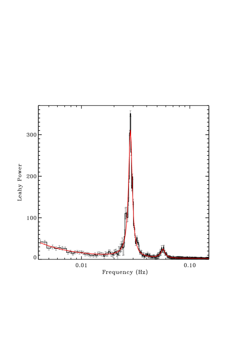
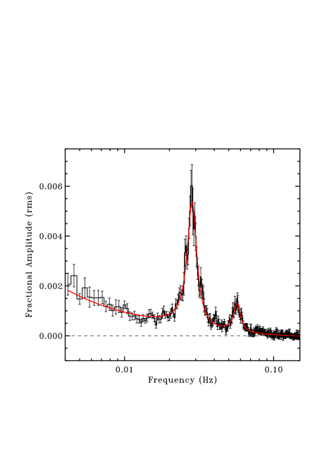
Figure 17: On the left, the power spectrum of the 24 continuous exposures longer than 1000 s (those in Table 5), and the best fit with the model parameters in Table 6. On the right, the average rms spectrum, computed by dividing each power spectrum by the mean count rate in each GTI and fitted with a two Lorentzian model.

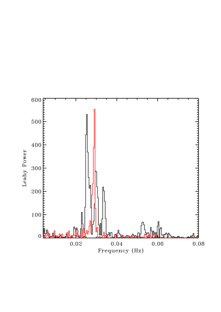
Figure 18: Comparison of the power spectra of the 9th GTIs (black) and the 22nd (red) of Table 5. Note that for purposes of comparison the spectrum for GTI 22 has been reduced by a factor of 2.5 to fit within the plotted range.

The light curves also suggest that the oscillation amplitude changes over periods of a few hundred seconds, ranging from a fractional amplitude (the sine wave amplitude relative to the mean) from less than 2% to a maximum of about 10%. In Fig. 17 we also show in the right-hand panel the average rms spectrum, computed by dividing each power spectrum by the mean count rate in each GTI and fitted with a two Lorentzian model. The parameters of the Lorentzian and first overtone are reported in Table 6. The rms amplitudes obtained from integrating the two Lorentzians are 9.41% and 3.08% (fractional rms) for the fundamental and 1st overtone, respectively. For several of the intervals with relatively ample oscillations with a single main peak in the power spectrum, the light curve can be folded at the best frequency, and an average QPO pulse profile is obtained. An example of this for the 17th GTI of Table 5 is shown in Fig. 19. The phase folded light curve shape slightly deviates from a simple sine wave, as a component at the first overtone frequency is required to adequately fit the data. In this case the relative amplitude of the fundamental and first overtone is 7.3.

Table 6: Model parameters for the fundamental and 1st overtone QPO peaks obtained from a fit to the average power spectrum shown in Fig. 17 (left).

QPO Component	$P_{max}$ (Leahy Power)	$\nu_{0}$ (mHz)	$\delta\nu$ (mHz)
Fundamental	$306.14\pm 4.31$	$28.316\pm 0.021$	$2.690\pm 0.055$
1st Overtone	$21.14\pm 1.70$	$56.600\pm 0.242$	$5.936\pm 0.679$

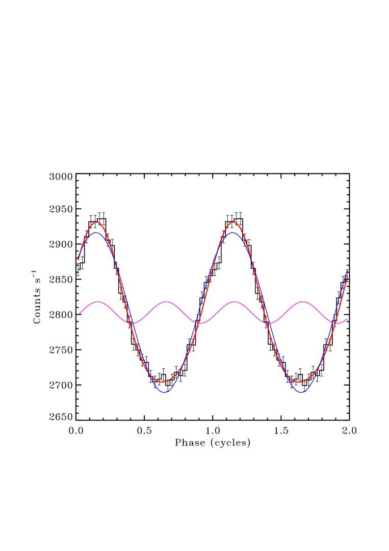
Figure 19: Folded QPO pulse profile for the 17th GTI of Table 5 fitted with a model that includes a sine function at the fundamental and the first overtone with relative amplitude of 7.3. The full model (red), fundamental (blue), and first overtone components (magenta) are also shown.

8.2 Statistical modeling of the short-term variability evolution

We have described above how in some GTIs the frequency seems stable, but in the majority of them, we measure a QPO rather than a stable period, given the apparent wandering of the frequency. Is it really a “QPO”? Sometimes the drift of the measured frequency is not real, but it is an artifact of the changing amplitude as in the case shown in Dobrotka & Ness (2017). In order to evaluate this possibility, we performed a statistical analysis, like previously done in Orio et al. (2021a) for N LMC 2009 and in Orio et al. (2022b) for CAL 83.

For this analysis we considered the light curves in the 0.2-0.6 keV range, in which the amplitude of the oscillation is the largest, and we used all continuous exposure times after the SSS emerged, longer than 700 s (that is, GTIs with at least 20 cycles). To detect and remove outlier points, we used the Hampel filter. For the light curve of each exposure, we computed an LS periodogram. We simulated the light curves using a sinusoidal function:

$$\psi=\phi+P_{a}\sin(2\pi t/P_{p}),$$ (3)

where $\phi$ is the mean GTI count rate, $P_{a}$ and $P_{p}$ are polynomials representing the amplitude and the period, respectively. Amplitude and period were obtained by generating a distribution of Gaussian points around their mean values in the selected GTIs. The mean modulation amplitude for each GTI was estimated from the phase-folded light curve by simple sine fitting, while the period was chosen randomly in the 20-40 mHz interval. We fitted the Gaussian random points with 25 degree polynomials, our input functions $P_{a}$ and $P_{p}$. When the modulated amplitude function $P_{a}$ turned out to be negative, we assumed P_a = 0 (a negative amplitude is meaningless), indicating that the modulation was below detection threshold for a while.

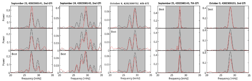
Figure 20: Examples of each type of variability with the best simulations (red lines) for the corresponding class of models. the top panels show stable periodicity with variable amplitude, the middle panels variable periodicity with stable amplitude, and in the bottom panels both parameters are assumed to be variable. For each observations, the best type of simulation is the one with the label ”Best”. We compare these simulations with the LS periodograms with $FAP>0.01$, traced in black. The sum of residual squares was calculated over the 10 mHz shaded interval around the peak.

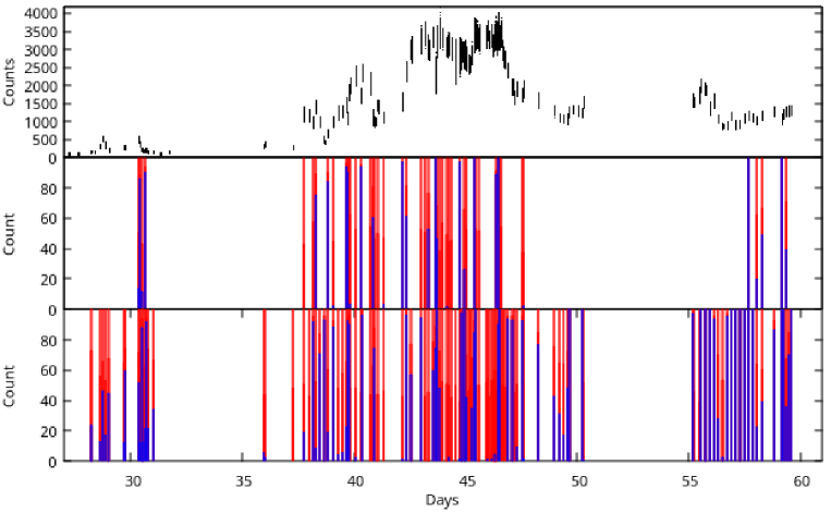
Figure 21: To visualize how the variability patterns changed during the NICER monitoring, the stacked bars show the number of best simulations (chosen from the best hundred out of 100,000) with each type of variability for each GTI: the number of best simulations with stable period and variable amplitude is plotted in blue, while the number of best simulations with variable period (or variable period and amplitude) is plotted in red. The upper panel represents the light curve for reference. The bottom panel shows the results for GTIs in which the signal was detected with $FAP<0.1$ and the middle panel shows the result for GTI exposures with $FAP<0.001$.

For three modes of variability (namely constant period with variable amplitude, variable period with constant amplitude, and variable both amplitude and period), and for each GTI, we run 100,000 simulations with relative LS periodograms to compare with the actual LS periodogram of each GTI exposure. We selected the best simulations for each GTI, by calculating the sum of square residuals in a 10 mHz interval around the highest peak (see shaded area in Fig. 20, that shows relevant examples). We chose GTI exposures done between days 30 and 60, in which the variability was well detected, and we selected those for which the periodogram has false alarm probability FAP$<$0.001. We chose the 100 best simulations (with lower residual squares) for every GTI, and plotted a stacked bar chart to visualize the fraction of simulations with and without varying frequency. This is shown in the middle panel of Fig. 21.

We considered that focusing only on the high confidence detections can lead to artificial selection of cases with non-varying amplitude, and we wanted to avoid a possible selection effect due to the fact that, if the amplitude varies, the peak power and its confidence may also decrease. Thus, we repeated the statistical analysis for GTI exposures done between day 26 and 60 with a minimal duration of 350 s (at least 10 cycles) and a less confident detection of the signal, FAP$<$0.1, increasing the number of examined GTIs. Because the GTIs with low confidence detection can be misleading due to random “noisy” peaks, we excluded those with periodograms that did not show the dominant feature around the 35 s periodicity. At the beginning, around day 30, there are solutions with both stable and variable period. Including the lower confidence data, the variability of the period is more obvious in the period of highest SSS flux, with practically no stable period solutions around days 41 and 44. Between days 55 and 60 the period seems to have stabilized, while the amplitude of the oscillation may have remained variable. We concluded that the 35 s period was becoming stable over the short time scale of minutes of the single GTIs in the late outburst phase, but it was indeed drifting over such scales early as the SSS emerged, and at peak SSS flux. Fig. 20 shows examples of the simulations for different dates. Periodograms with stable periodicity have a typical single peak (see September 25th and October 9th). These simulations generate blue bars in Fig. 21. We see in the top panel for October 8th that the simulations with stable period and variable amplitude split the signal into two peaks, but the solution with variable frequency (middle panel) is a better match. Both simulated solutions are very similar, and the difference is in the amplitude of the peaks. Both models, with variable or stable frequency, may describe the observed periodograms relatively well and can be counted among the selected best 100 cases. For this reason there are partially blue and partially red bars for most dates in Fig. 21, but a GTI like the one whose power spectrum is plotted in black in Fig. 18 generates almost only blue bars in Fig. 21.

8.3 Long-term variability of the 35 s signal

In addition to testing the drift of the period on time scales of minutes of the individual GTIs, we also wanted to investigate whether the mean period appears to be stable on long term time scales and/or whether there is any trend towards longer or shorter periods. We selected the most stable GTIs, namely those with at least 90 (out of 100) stable-period-simulations fitting the measured periodogram, defined by almost entirely blue bars in the middle panel of Fig. 21. This left us with only 8 GTIs (out of the 24 in Table 5) for which we can assume that there was no significant frequency drift. We evaluated the statistical error of the frequency by fitting Gaussians to the periodogram peaks and considering 1$\sigma$. The result is plotted in the top panel of Fig. 22. There is no clear trend: we notice that there is still variability on this time scale of days, although there is only a significantly different (larger) frequency at the beginning, on day 30. We also calculated a periodogram (to compare with the average power spectrum of the 24 GTIs of Table 5, shown above in Fig. 17) using only these ”most stable, bluest” GTIs, and the result is shown in the middle panel. The frequency measured using all the 8 stable-period GTIs is 27.8862$\pm$0.0012 mHz, corresponding to an average period of 35.86 s. Using instead all the GTIs of Table 5 (all long, uninterrupted ones), as reported above we obtained a fundamental frequency of 23.316$\pm$0.021 mHz, corresponding to a 35.316 s period. The frequency of the combined “mostly red/drifting” GTIs is instead 28.5062$\pm$0.0009 mHz, corresponding to an average period of 35.08 s. When we compared the phased light curves of the stable GTIs with the “red” ones with large period drifts on time scales of minutes, in the bottom panel for Fig. 21, we found a much smaller amplitude (and a less definite shape) of the modulation for the “red” GTIs, the ones with a significant period drift, supporting the conclusion that the drift in period in those GTIs is real and we can really define this modulation a QPO. To summarize, we suggest that the period drift on short time scales of minutes is real, and that it was also not stable over time scales of days. The only long term trend we could assess as the days passed is that fewer GTIs showed the period drift. Although comparing the frequency obtained from the power spectrum of the single GTIs does not yield conclusive results, this decreasing drift may mean that the QPO was becoming a fixed period at the later epochs.

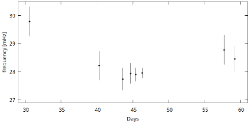
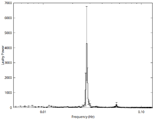
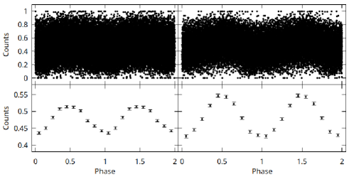
Figure 22: The top panel compares the frequency measured for the 8 GTIs without significant period drift. The middle panel shows the periodogram measured for these 8 GTIs, yielding a period of 35.87 s (see text). The bottom panel shows the phased light curves, with a 1 s bin, of the drifting-period “red GTIs on the left, and that of the 8 stable-period “blue” GTIs on the right. The data points were folded in the bottom panel with the 35.08 s period and with the 35.87 s periods, respectively. The count rate was normalized by the highest measured, and below we binned the data in bins of 0.1 times the phase (10 per cycle) and plotted the average count rate in each bin.

9 The final decline

The around-peak count rate was measured between day 45 and 59, still with significant variability, and after day 55 it decreased. Daily observations had to be interrupted twice for technical reasons, once between days 51 and 57 (September 29 and October 5) and again between days 64 and 67 (October 12 and October 15). Although on day 51 a new moderate rise was measured, after day 67 there was a constant decrease with lower irregular variability amplitude.

As the angular distance to the Sun decreased ($\leq 60^{\rm o}$), there was significant optical loading in the softer energies. After day 67 we had to disregard the 0.2-0.3 range, and towards the end of October the optical loading became more and more severe with spurious flux leaking up to 0.4-0.5 keV. The exposure ceased early in November, with the last one on November 6 (day 89). Thus, like the optical monitoring, X-ray monitoring had to end sooner in 2006 than in 2021 for the Sun constraint.

As the luminous supersoft X-ray source was fading, emission lines were still clearly detected with NICER, with a spectrum indicating decreasing plasma temperature. As the SSS was becoming less and less luminous, like in the initial phases of the rise, discriminating between the contribution of an atmosphere and a luminous component of very soft plasma was not possible, also because we could not resolve and measure emission lines in the softest range above the still strong continuum. While on day 67 in 2021 the NICER estimated flux was only 2.15 $\times 10^{-10}$ erg cm^-2 s^-1, on day 67 of the 2006 outburst (2006 April 20) the measured X-ray flux with the Chandra LETG grating was still 3.8 $\times 10^{-9}$ erg cm^-2 s^-1, a factor of 47 higher (Nelson et al., 2008). Our model fits to the NICER data (see Table 2) show that this very large difference is not explained with larger column density in 2021. Indeed, the absolute flux must have been much lower at this stage in 2021 than in 2006.

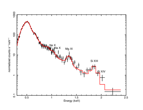
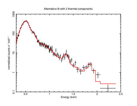
Figure 23: The average spectrum observed on 2021 October 28, and the fit with two composite model: a stellar atmosphere and a BVAPEC thermal component (left), and two BVAPEC thermal components (left). Both fits yield $\chi^{2}$/d.o.f.=1.4, and are virtually indistinguishable.

Two models for October 28 (day 80) are shown in Fig. 23 We constrained the column density value to be at or above 2 $\times 10^{21}$ cm^-2, and thus the fit to the softest portion (0.3-0.5 keV) is not perfect, but we attribute the discrepancy mainly to the optical loading contamination. Another imperfection of the fit may be due to strong He-like lines of Na X (the Na abundance is not included vary in the XSPEC BVAPEC model). However, both fits are statistically reasonably good, with $\chi$/d.o.f=1.5. At a distance of 2.4 kpc distance. the thermal plasma would have a very large absolute luminosity of 6.1 $\times 10^{35}$ erg s^-1, close to the value obtained for the early days of the outburst, when the emission was much “harder”. This seems hardly consistent with the previously observed flux decrease of the cooling shocked plasma, and it would imply considerable renewed mass ejection should have occurred long after after the initial outburst, which seems unlikely, also because there are no signatures of such an event in the optical spectra,

On the other hand, the atmospheric component would emit 2.3 $\times 10^{35}$ erg s^-1, but the effective temperature resulting from the fit is 564,000 K. With this temperature, most of the WD bolometric luminosity is emitted the X-rays, but the radius of the emitting region with this luminosity would be only 5.7 $\times 10^{7}$ cm, only a small fraction of a WD radius. Recent observational estimates of WD radii are found in Bédard et al. (2017): for instance, the radius of a WD of 1.13 M_⊙ is about 5.3 $\times 10^{8}$ cm^-2. The WD of RS Oph may be even more massive, but it is very unlikely that its radius is so small. This may imply that we are not seeing the whole area of the WD emitting as an SSS, either because of new, large clumps that are opaque to soft X-rays, which seems unlikely at this stage, or because only part of the surface is emitting as an SSS.

Above $\simeq$ 1 keV, where the SSS continuum is not dominant and the spectral resolution of NICER is quite good, the spectrum still shows prominent emission lines. There is evidence that in 2006, the emission due to shocks faded much later than the SSS. In fact, A late-epoch high resolution X-ray spectrum measured with the Chandra LETG and HRC-S camera on 2006 June 4 (day 104 of the outburst) (Nelson et al., 2008) is shown in Fig. 24. The figure also shows a fit, that constrains the column density to be N(H)$\leq 2\times 10^{21}$ cm^-2. Two components of thermal plasma in equilibrium are assumed, at $\simeq$240 and $\simeq$630 eV (the fit with two regions explains most, but not all emission lines, however we did not want to introduce many free parameters). It is clear that there was still a considerable region of shocked material even at such post-outburst epochs in 2006, so the emission of the shocks faded much later than the SSS.

10 Discussion

We summarize and discuss in this section some important points resulting from our data analysis.

$\bullet$ The rise of the X-ray light curve in the 0.2-10 keV range due to the optically thin thermal emission of shock-heated plasma lasted until the 5th post-outburst day, and a slow decline followed until the beginning of a “mixed” phase in the fourth week, when supersoft flux started to emerge. Our spectral fits imply that the peak of the plasma temperature was close to 27 keV already at the end of the second day, as the unabsorbed and absorbed flux were still rising.

$\bullet$ In the first week, the spectrum can always be fitted with temperature higher than 5 keV. The total flux in He-like features is quite higher than that in the H-like lines, while at such high temperature the emitting plasma should be almost completely ionized if it is in CIE. We experimented with several combination of models and found that we cannot fit the early X-ray spectra with two or more regions in CIE. We suggest that the plasma was not in equilibrium until at least day 5. Between days 6 and 12, we could fit the spectra equally well with a combination of two thermal plasma regions at different temperature, either in CIE or NEI, but we find the BVAPEC model more likely to be realistic, because the NEI assumption requires a very high column density parameter, so the absolute flux turns out to be super-Eddington. Moreover, we obtain inconsistent values for the electron density. We also found that until day 12, the best fits are obtained assuming also a partially covering absorber with large column density, covering from 70% to 40% of the surface, slowly decreasing in time.

$\bullet$ Towards the end of the third week, three components are necessary for spectral fits. Two of these components are still modeled with the BVAPEC thermal plasma in CIE. In the following two weeks, the emerging SSS flux can be fitted equally well by adding a third component, which may be stellar (blackbody or atmospheric model), or a thermal plasma at temperature kT$\leq$100 eV. In the initial SSS rise, either we did not observe emission from all the WD surface, or only new layers of less hot, either shocked or photoionized ejected material near the WD were becoming visible before the WD itself. Our data do not have the spectral resolution to distinguish between the two cases.

$\bullet$ The large SSS variability at peak luminosity, with soft flares lasting for a few hours, is not explained with varying column density. The best fits to the initial in-flare and out-of-fare spectra seem to imply that the SSS flux suddenly increased for short periods because a larger emission region became visible. After a large rise around day 37, the circumstellar material became permanently optically thin for soft X-rays and the soft X-ray flux was consistent with an origin from all the WD surface. However, aperiodic variability persisted. We refer to Ness et al. (2022a), who compared a high resolution X-ray SSS spectrum of 2021 with two taken in 2006, concluding that the SSS variability is due to changes in the ionization stage of the absorbing medium near the source. Variations in an O I absorption edge explain most spectral differences; they may be due to a inhomogeneous outflow from the nova. The NICER data confirm that we cannot attribute the flux variations to other phenomena, specifically not to variations in blackbody/atmospheric temperature, changes in column density, or a dust scattering halo.

$\bullet$ Page et al. (2022) suggested that the Swift XRT spectra indicate that after day 60 were “hotter, with smaller effective radii and lower wind absorption”. The model by Page et al. (2022) does not yield a good fit to the more structured NICER spectra, so we cannot support this conclusion. On the other hand, the example of a comparison shown in Fig. 12 of a NICER spectrum and a pile-up corrected Swift XRT one for day 57 of the outburst demonstrates that the spectrum extracted from a smaller region than the whole PSF, omitting the PSF center, results in a fit (either with an atmospheric or a blackbody model) converging at higher column density and temperature than the fit the NICER spectrum of the same day. Thus, the parameters derived from the Swift XRT spectra in this phase may be an artifact of the “partial” extraction region method, that is necessary to avoid pile-up, but does not provide an estimate of the actual flux for the normalization of the adopted model.

$\bullet$ The NICER spectra indicate a general trend of SSS cooling, albeit a moderate one, on day 67 after an interruption in the monitoring. The decrease in luminosity does not appear in the model fits to be only due to cooling, and we inferred that the SSS emitting region was shrinking. There is also no indication that the decline in luminosity was due to a sudden increase in column density, a possibility discussed - but not found to be supported by the data - by Page et al. (2022). We note that several novae, particularly magnetic ones (intermediate polars) which may already have hotter polar regions at the onset of the outburst, have been found to fade at almost constant temperature in the X-rays: V2491 Cyg (Page, 2012), V4743 Sgr (Zemko et al., 2016), V407 Lup (Aydi et al., 2018), V1674 Her (Orio et al., 2022b).

Page et al. (2022); Ness et al. (2022a) discussed how the [Fe X] coronal emission line detected in optical mimicked the light curve and the decay of the SSS in 2006 (but there are only sparse data for the actual trend of this line in 2006) and how this may indicate the same cooling time and duration of the central photoionizing source in 2006 and 2021, despite the faster decay of the SSS. The line is due to a ${}^{2}P_{1/2}=>^{2}P_{3/2}$ transition of Fe⁹⁺, a ion with a ionization potential of 233.6 eV. It indicates high temperature and it can be either formed by photoionization very close to the central source, or by shock ionization anywhere in the ejecta. The evolution of the [Fe X] line flux was accurately monitored in 2021 (see Page et al., 2022) and does not follow the SSS light curve of 2021. Ness et al. (2022a) thus suggested that the SSS decline of the in 2021 may not have been more rapid than in 2006, and that part of the SSS emitting region may have been blocked from the line of sight at late epochs. The reasoning is that the [Fe X] line is due to photoionization by the central source in the ejecta, while occulting blobs of matter obscured only the supersoft X-rays. The complex geometry that would be required for the SSS flux to be photoionizing (visible) ejecta that should be very close to it, without being observable any more along the line of sight, is not discussed in the paper. We suggest instead a simpler interpretation: still shocked ejecta present during the SSS turn-off in 2021 (as well as even later in 2006) indicate shock ionization, rather than photoionization also for the [Fe X] line at this stage in the outburst. We do not rule out a large contribution of photoionization in the formation of this line in earlier phases, but we suggest that the [Fe X] line is not due photoionization by a still hot central source (due to hidden, ongoing nuclear burning) during the late decline.

We concluded that the SSS did actually turn off after day 60. In Fig. 24, we supported our conclusion by presenting the Chandra HRC-S+LETG high resolution spectrum of RS Oph on day 114 of the outburst, 2006 June 6 (see also Nelson et al., 2008). At the same epoch in the outburst, RS Oph was close to the Sun in 2021 and could not be observed. Several emission lines in the X-ray range were still consistent with being due to shock ionization and we suggest that the [Fe X] line most likely originated in the same medium. Furthermore, still as late as on day 201 in the 1985 outburst, when the [Fe X] line had already disappeared, many other lines in the optical range were still due to shock ionization (Contini et al., 1995).

On day 67 of the 2021 outburst, October 15, the absorbed flux obtained in our fits is about 2.5 $\times 10^{-10}$ erg cm^-2 s^-1, while on day 67 of 2006 (April 20 2006) the measured flux with the LETG Chandra X-ray grating was still 3.8 $\times 10^{-9}$ erg cm^-2 s^-1 (Nelson et al., 2008), a factor of 15 higher than at earlier epoch in 2006, too large a difference to be explained with partial obscuration by an opaque cloud or clump. Furthermore, even if we did not achieve rigorous spectral fits for the SSS in the most luminous period, the “qualitatively best” fits are consistent with cooling after day 67. We could not prolong the observations during complete turn off of the SSS, as it was possible back in 2006, but the constant decrease rate in SSS flux and the large difference with respect to the 2006 flux at the same post-outburst stage indicate that, when our NICER observations ended at day 89, the SSS was already switching off and the SSS phase was quite shorter in 2021 than in 2006.

$\bullet$ We would like to compare RS Oph with the ”sister system” V3890 Sgr. V3890 Sgr is a symbiotic at a distance of 4.2 kpc, with a later spectral type M giant than RS Oph, M5 III (Anupama & Mikołajewska, 1999). Its recurrent nova outbursts were observed in 1962, 1990 and 2019. The main known differences from RS Oph are the longer recurrence time, about 29 years, and the more rapid development and turn-off in X-rays, despite an optical light curve that was very similar to RS Oph. Given the shorter recurrence time of RS Oph, we may expect it had a larger average mass accretion rate. The X-ray spectrum of the shocked plasma of V3890 Sgr on day 7 was well fitted with two thermal components in collisional ionization equilibrium at temperatures of 1 keV and 4 keV (Orio et al., 2020), close to values obtained for RS Oph around day 10-11. The SSS in V3890 Sgr rose to maximum already on the 9th day and declined within 26 days (Singh et al. 2021; Ness et al. 2022b); the effective temperature was between 820,000 K and 950,000 K (Singh et al. 2021). Thus the SSS was shorter lived and probably hotter than in RS Oph, and the models predict that these parameters indicate an even higher mass WD than the (already high) mass of the RS Oph WD. Both should be quite close to the Chandrasekhar mass (Yaron et al. 2005)

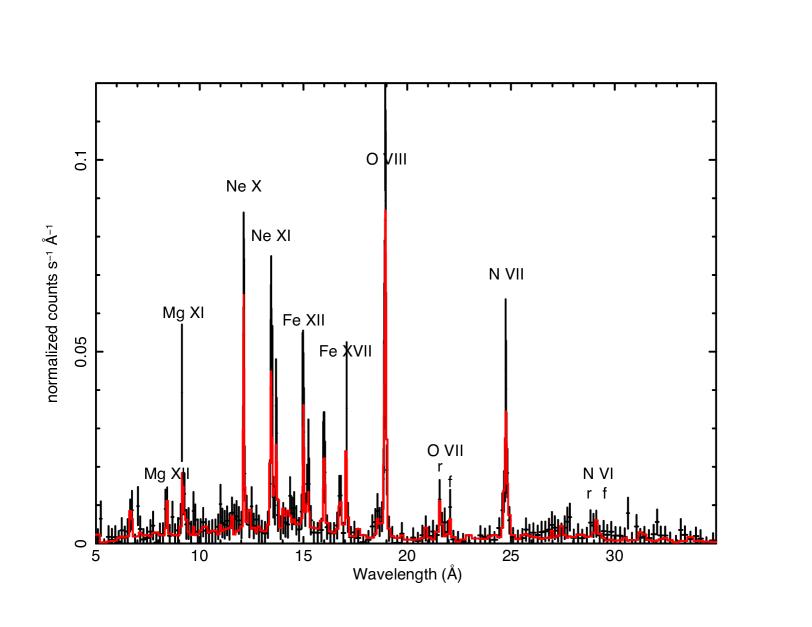
Figure 24: The spectrum observed with the Chandra LETG grating and the HRC-S camera on 2006 June 6, and a fit with two components at thermal plasma at 240 eV and 630 eV, with N(H)=2.2 $\times 10^{21}$ cm^-2 and moderately enhanced abundances except for iron (which is only 15% the solar abundance).

11 Conclusions

RS Oph was monitored with NICER in its 2021 nova outburst from the second day of the outburst until day 89, when it was too close to the Sun. Monitoring occurred in $\simeq$1 ks exposures almost every day, and often several times a day, producing an exquisite dataset of high quality. Because this was the second outburst of this recurrent nova monitored in X-rays, we can also learn much from the comparison between outbursts. Moreover, other observations were done at all wavelengths, from high energy gamma rays to radio.

1. With RS Oph, we obtained for the first time simultaneous data with high S/N in both X-rays and gamma rays. In the first three weeks, the X-ray rise to maximum took about four days, while in optical and in gamma rays in the Fermi range (peaking around 1 GeV, see Cheung et al., 2022) the peak was observed at the end of the second day. The AAVSO light curve shows an extremely rapid rise from optical magnitude V$\simeq$9 to almost V$\simeq$5 magnitude within few hours, and a subsequent rise to V$\simeq$4.2 within the next day. The flux observed with the H.E.S.S. Cherenkov telescope, on the other hand, reached maximum on the fourth day, with peak energy about 100 GeV (H. E. S. S. Collaboration, 2022). If we consider the shock temperature instead of the X-ray flux, the best model fits indicate that the plasma temperature was already peaking at $\simeq$27 keV at the end of day 2.

The gamma rays in novae have been attributed to either inverse Compton effect or proton acceleration following the powerful shocks between different ejecta, or between the ejecta and the circumstellar environment. Typical nova outflow velocities are such that the regions of the shocks emit X-rays. It is reasonable to assume radiative shocks (see Diesing et al., 2022), in which the velocity of the shock speed is proportional to the temperature as kT $\simeq$ 1.2 (v/1000 km s${}^{-1})^{2}$ (Mabey et al., 2020). The maximum temperature of 27 keV that we obtained, corresponds to a shock velocity around 4750 km s^-1. Diesing et al. (2022), among others, suggested that in symbiotic novae like RS Oph with dense pre-existing red giant wind are likely to be due to proton accelerations. This is the so-called “hadronic” mechanism in which protons collide with neutrons or ions, and pions are generated. The neutral pions decay, producing gamma rays. Secondary X-ray emission, namely the X-ray tails of the phenomena emitting gamma rays, is predicted with a non-thermal component, but Vurm & Metzger (2018) find that only a small fraction, of order 10${}^{-4}-10^{-3}$ the gamma ray luminosity is radiated in X-rays above 10 keV (and even much less is radiated below 10 keV). Nelson et al. (2019), among others, pointed out that all X-rays emission (primary and secondary) must have been in a very absorbing medium because very little or no X-ray flux was detected simultaneously with the gamma rays before this recent outburst of RS Oph.

Diesing et al. (2022) found that the Fermi and H.E.S.S. light curves are not compatible with an origin in the same shock, and that two or more shocks must have occurred. Given the time scales, the X-rays we measured with NICER below 12 keV are more compatible with H.E.S.S. We notice that the flux ratio of the maximum NICER flux to the peak H.E.S.S. flux (integrated from about 250 GeV and 2.5 TeV) is about 100, and the ratio of soft X-rays to the Fermi flux (integrated between 60 MeV and 500 GeV) is almost an order of magnitude higher than the flux measured with NICER. However, there is no signature for RS Oph of the predicted, accompanying non-thermal emission in the NICER and NuSTAR ranges (see Luna et al., 2021, for the latter,) namely the “tail” of the gamma-ray flux at lower energy. This implies that, despite the high thermal X-ray flux compared to the gamma-ray flux, the lower limit ratio of non-thermal X-rays to gamma rays flux (measured in the Fermi energy range) is orders of magnitude lower than indicated by upper limits and detections measured for many classical novae (Metzger et al., 2015; Nelson et al., 2018b, a, 2019; Sokolovsky et al., 2023) and even less than the factor of 10${}^{-4}-10^{-3}$ expected for the secondary emission above 3 keV. It is thus possible that the X-rays we observed were altogether from a completely different region than the original shocks that caused particle acceleration.

2. Modeling the shocks observed in X–rays, their the nature and sites is critically dependent on accurate estimates of the plasma temperature. For most GTIs in the first 5.5 days, we find a good fit only by modeling the spectrum as a thermal plasma that has not yet reached CIE. We obtain fits that are compatible with the ones to the SWIFT XRT spectra, requiring two thermal components, only from day 6 and can completely rule out the NEI models only from day 12. However, we caution that the NEI models yield values of the electron density obtained from the ionization time scale, that are not consistent with the lower limits given by the emission measures, even assuming the extremely high velocity inferred in the radio in the first days (the optical spectra indicate a lower peak velocity, around 2800 km s^-1). With Swift the emission lines were either not resolved, or resolved with a small S/N ratio, so CIE models yielded a good fit from the beginning, but NICER presents a more complex picture.

3. It is not surprising that the spectra of the shocked gas cannot be fitted with only one region at uniform temperature already from day 2, because two or more plasma temperatures have often been found necessary to fit the early X-ray spectra of both recurrent and classical novae (Drake et al., 2016; Peretz et al., 2016; Orio et al., 2020). For classical novae, the shocks are thought to be due to colliding winds from the nova at different velocity; perhaps at the intersection of a fast polar outflow with a slower expanding torus of material around the WD (e.g. Chomiuk et al., 2021), while for symbiotic novae the shock has been mainly attributed to the impact of the fast nova wind with the less dense and much slower pre-existing red giant wind, especially in the equatorial plane (see Orlando et al., 2009). However, in RS Oph the scenario may be even much more complex, with multiple shock sites. In symbiotics, in fact, shocks may also occur near the red giant, which subtends a large angle, and/or in the impact with the accretion disk (when present). Diesing et al. (2022) invoke two different shocked region to explain the gamma rays of RS Oph in different energy ranges, that of Fermi and that of the Cherenkov telescopes. At the same time, as outlined above, the absence of even a low-flux non-thermal component in the 3-79 keV range of NuSTAR, namely the “low energy tail” of the flux measured in the gamma rays exposures (done while high gamma ray flux was still detected Luna et al. 2021), suggests that the shocks we observed with NICER may even not be related to those that caused the gamma ray emission. It is also very interesting to note that, by examining the coronal lines of [Fe X], [Fe XIV] and [Ca XV] in published optical spectra of RS Oph in the outbursts of 1958 and 1969, Cassinelli (private communication) found that the ratios of the fluxes in these forbidden lines are not consistent with each other, indicating out at an origin in at least two different region of shocks, with material at different velocity and temperature.

4. Towards the end of the third week a third plasma component is necessary for the fit, and the spectrum became difficult to interpret as the supersoft flux increased. For a period of at least 10 days, fits with a blackbody (or a WD atmosphere) as third component are equally good as the fits with a third thermal component in the softest range, around 80-90 eV. This outlines the possibility of confusion and related uncertainty in determining an exact SSS turn-on time with broad-band X-ray spectra. X-ray grating spectra of RS Oph published by Orio et al. (2022a) show that supersoft flux on day 21 was due to an emission line spectrum. On day 26(September 4), the 35 s pulsation appeared, probably indicating that at this stage the stellar surface became visible, at least partially. We thus conclude that the ejecta became optically thin to the WD emission between these two post-outburst dates, day 21 and 26 (August 30 and September 4). The general assumption is that the source of the supersoft flux is the WD atmosphere, or layers being detached from it, but still very close to the WD (e.g. Rauch et al., 2010). The material is extremely hot because nuclear burning is still ongoing at the bottom of the accreted envelope, with only a thin layer above it. The time it takes for the SSS to become detectable may be interesting quantity because, at least in an “ideal world” in which the ejecta are spherically symmetric and are outflowing with constant velocity, is proportional to the mass of the ejecta, which cause intrinsic absorption before they expand enough to be transparent to the SSS.

5. The turn-off time is probably an even more important quantity, because the models predict that it should be directly proportional to the leftover hydrogen mass, which is roughly directly proportional to the initially accreted envelope. Moreover, the models also predict that WD mass is inversely proportional to the effective temperature, because a thinner layer is left on a more massive WDs (Yaron et al., 2005; Starrfield et al., 2012; Wolf et al., 2013). We find that the blackbody temperature for the SSS fits with variable abundance in the interstellar medium is in the 35-40 eV ($\approx$ 405,000-470,000 K) range (consistently also with Swift, for which of ad-hoc absorption edges were superimposed on the blackbody Page et al., 2022). According to Wolf et al. (2013) this is the peak temperature of a 1 M_⊙ WD after the outburst. However, the effective temperature of the WD atmosphere is quite higher than a blackbody of with the same X-ray luminosity (see Heise et al., 1994; Starrfield et al., 2012; Wolf et al., 2013); although we could not obtain a rigorous fit with the (limited) public model grid, the fits tend to converge at about $\simeq$750,000 K ($\simeq$65 eV), predicted to be the peak temperature of a 1.2 M$\odot$ WD (Wolf et al., 2013).

We also established that between days 75 and 89 the SSS was already cooling off and its flux was rapidly decreasing. We presented evidence that this has to be interpreted as a real switching-off of nuclear burning, rather than a temporary obscuration by increased, large column density (a possibility hypothesized by Page et al., 2022; Ness et al., 2022a). A turn-off time around 85 days in the models is associated with a WD mass close to 1.3 M_⊙ (Wolf et al., 2013). After day day 67, we also found evidence that the cooling was accompanied by a shrinking of the emitting region. At this stage, we did not observe irregular variability any more, and there was only a constant decrease in X-ray luminosity. The fact that shocked plasma was still detected until the last day (day 89) and was present even later in outburst phase in 2006, points out at the [Fe X] coronal emission line in the optical region as having its origin - at least in the late outburst phase - in shocked ejecta, instead of being an indicator of a central photoionizing source.

6. Another example of very similar optical light curves, yet with quite a different development in X-rays, is the one of V3890 Sgr, described in Section 10. Therefore, it is not entirely surprising that the X-ray lightcurves of RS Oph in 2006 and in 2021 were different. The previous RS Oph outburst occurred after 21 years, the recent one after 15: probably, the bottom shell of the WD envelope was sufficiently hot and electron-degenerate to allow the thermonuclear runaway with a smaller envelope mass. It is possible that recurrent novae explode with lower and lower accreted mass as they evolve in time. In fact, we note that also the recurrent nova U Sco in its 2022 outburst had a more rapid SSS phase than in 2010 (Zhang et al. 2023, article in preparation).

The fact that the optical light curves of RS Oph in 2006 and 2021 were virtually “clones” of each other, while the X-ray light curve shows a much shorter SSS phase, is extremely interesting because the SSS is the only indication we have of thermonuclear burning. The mass ejected following the thermonuclear runaway in RS Oph may have been quite smaller than in 2006, but the almost identical optical peak luminosity and decay rate indicate that there must be another important mechanism powering the optical luminosity. This mechanism is likely to be the reprocessing of the X-ray flux into optical light, inferred for nova V906 Car by Aydi et al. (2020) and previously also suggested for nova V1324 Sco Metzger et al. (2014). Although detailed calculations are not available yet, Metzger et al. (2015) presented a phenomenological estimate, confirming this scenario. We suggest that also in RS Oph powerful shocks, like those we probed in X-rays but not necessarily in the same sites, are fundamental in shaping also the optical characteristics and parameters. This implies that the optical decay rate (specifically, the time for optical decay by 2 and 3 magnitudes, t₂ and t₃) may not be indicative of the nova absolute luminosity (hence, its distance) and of the WD mass as previously thought. Furthermore, mass loss via Roche Lobe overflow in the common envelope phase may have contributed to the optical phenomenology, even if the accumulated envelope was smaller (possibly, because the temperature on the WD surface increased after the previous outbursts), while the initial radiation driven wind carried away a lower amount of mass in 2021 (see nova mass loss models by Shen & Quataert, 2022).

7. The $\simeq$35 s quasi-periodic pulsation, identical in the 2006 and 2021 outbursts, must be an intrinsic property and is most likely related to the WD and/or its shell thermonuclear burning. The coincidence of a QPO of exactly the same duration of $\simeq$35 s in another nova in the SSS phase (KT Eri, see Ness et al., 2015) is suggestive of a stellar pulsation. While in other X-ray data (of RS Oph in 2006 and other novae, see Ness et al., 2015) the period of the SSS flux oscillations does not appear to be clearly detectable in the whole SSS phase, NICER has demonstrated that although the amplitude varies (yielding a non-detection with less sensitive instruments), the semi-periodicity is always present as long as the SSS is luminous. With a statistical analysis, we also found evidence that the period drift decreased toward the end of the SSS phase and the period tended to stability.

Finally, we would like to conclude pointing out the characteristics of NICER that allowed gathering this beautiful and very useful data set: high S/N without pile-up problems that make it very suitable to study the SSS, the possibility to study some emission line ratios, and the timing capabilities. In the future, NICER will continue to prove an invaluable instrument to examine the nova mysteries connected to fundamental physical processes.

References

- Acciari et al. (2022) Acciari, V. A., Ansoldi, S., Antonelli, L. A., et al. 2022, Nature Astronomy, 6, 689, doi: 10.1038/s41550-022-01640-z
- Anupama & Mikołajewska (1999) Anupama, G. C., & Mikołajewska, J. 1999, A&A, 344, 177. https://arxiv.org/abs/astro-ph/9812432
- Arnaud (1996) Arnaud, K. A. 1996, in Astronomical Society of the Pacific Conference Series, Vol. 101, Astronomical Data Analysis Software and Systems V, ed. G. H. Jacoby & J. Barnes, 17
- Aydi et al. (2018) Aydi, E., Orio, M., Beardmore, A. P., et al. 2018, MNRAS, 480, 572, doi: 10.1093/mnras/sty1759
- Aydi et al. (2020) Aydi, E., Sokolovsky, K. V., Chomiuk, L., et al. 2020, Nature Astronomy, 4, 776, doi: 10.1038/s41550-020-1070-y
- Bailer-Jones et al. (2021) Bailer-Jones, C. A. L., Rybizki, J., Fouesneau, M., Demleitner, M., & Andrae, R. 2021, AJ, 161, 147, doi: 10.3847/1538-3881/abd806
- Barry et al. (2008) Barry, R. K., Mukai, K., Sokoloski, J. L., et al. 2008, in Astronomical Society of the Pacific Conference Series, Vol. 401, RS Ophiuchi (2006) and the Recurrent Nova Phenomenon, ed. A. Evans, M. F. Bode, T. J. O’Brien, & M. J. Darnley, 52
- Bédard et al. (2017) Bédard, A., Bergeron, P., & Fontaine, G. 2017, ApJ, 848, 11, doi: 10.3847/1538-4357/aa8bb6
- Bode (1987) Bode, M. F. 1987, RS Ophiuchi (1985) and the recurrent nova phenomenon. Proceedings of the Manchester Conference, held at Manchester, UK, 16 - 18 December 1985.
- Bode et al. (2006) Bode, M. F., O’Brien, T. J., Osborne, J. P., et al. 2006, ApJ, 652, 629, doi: 10.1086/507980
- Borkowski et al. (2001) Borkowski, K. J., Lyerly, W. J., & Reynolds, S. P. 2001, ApJ, 548, 820, doi: 10.1086/319011
- Brandi et al. (2009) Brandi, E., Quiroga, C., Mikołajewska, J., Ferrer, O. E., & García, L. G. 2009, A&A, 497, 815, doi: 10.1051/0004-6361/200811417
- Brickhouse et al. (2005) Brickhouse, N. S., Desai, P., Hoogerwerf, R., Liedahl, D. A., & Smith, R. K. 2005, in American Institute of Physics Conference Series, Vol. 774, X-ray Diagnostics of Astrophysical Plasmas: Theory, Experiment, and Observation, ed. R. Smith, 405–407, doi: 10.1063/1.1960961
- Cheung et al. (2022) Cheung, C. C., Johnson, T. J., Jean, P., et al. 2022, arXiv e-prints, arXiv:2207.02921. https://arxiv.org/abs/2207.02921
- Chomiuk et al. (2021) Chomiuk, L., Metzger, B. D., & Shen, K. J. 2021, ARA&A, 59, 391, doi: 10.1146/annurev-astro-112420-114502
- Contini et al. (1995) Contini, M., Orio, M., & Prialnik, D. 1995, MNRAS, 275, 195, doi: 10.1093/mnras/275.1.195
- Corrales et al. (2016) Corrales, L. R., García, J., Wilms, J., & Baganoff, F. 2016, MNRAS, 458, 1345, doi: 10.1093/mnras/stw376
- Diesing et al. (2022) Diesing, R., Metzger, B. D., Aydi, E., et al. 2022, arXiv e-prints, arXiv:2211.02059. https://arxiv.org/abs/2211.02059
- Dobrotka & Ness (2017) Dobrotka, A., & Ness, J. U. 2017, MNRAS, 467, 4865, doi: 10.1093/mnras/stx442
- Dobrzycka et al. (1996) Dobrzycka, D., Kenyon, S. J., Proga, D., Mikolajewska, J., & Wade, R. A. 1996, AJ, 111, 2090, doi: 10.1086/117945
- Dorman & Arnaud (2001) Dorman, B., & Arnaud, K. A. 2001, in Astronomical Society of the Pacific Conference Series, Vol. 238, Astronomical Data Analysis Software and Systems X, ed. J. Harnden, F. R., F. A. Primini, & H. E. Payne, 415
- Draine (2003) Draine, B. T. 2003, ApJ, 598, 1026, doi: 10.1086/379123
- Drake et al. (2009) Drake, J. J., Laming, J. M., Ness, J. U., et al. 2009, ApJ, 691, 418, doi: 10.1088/0004-637X/691/1/418
- Drake et al. (2016) Drake, J. J., Delgado, L., Laming, J. M., et al. 2016, ApJ, 825, 95, doi: 10.3847/0004-637X/825/2/95
- Evans et al. (2007) Evans, P. A., Beardmore, A. P., Page, K. L., et al. 2007, A&A, 469, 379, doi: 10.1051/0004-6361:20077530
- Fajrin et al. (2021) Fajrin, M., Imaduddin, I., Malasan, H. L., et al. 2021, The Astronomer’s Telegram, 14909, 1
- Ferrigno et al. (2021) Ferrigno, C., Savchenko, V., Bozzo, E., et al. 2021, The Astronomer’s Telegram, 14855, 1
- Franckowiak et al. (2018) Franckowiak, A., Jean, P., Wood, M., Cheung, C. C., & Buson, S. 2018, A&A, 609, A120, doi: 10.1051/0004-6361/201731516
- Fruscione et al. (2006) Fruscione, A., McDowell, J. C., Allen, G. E., et al. 2006, in Society of Photo-Optical Instrumentation Engineers (SPIE) Conference Series, Vol. 6270, Society of Photo-Optical Instrumentation Engineers (SPIE) Conference Series, ed. D. R. Silva & R. E. Doxsey, 62701V, doi: 10.1117/12.671760
- H. E. S. S. Collaboration (2022) H. E. S. S. Collaboration. 2022, Science, 376, 77, doi: 10.1126/science.abn0567
- Hachisu et al. (2007) Hachisu, I., Kato, M., & Luna, G. J. M. 2007, ApJ, 659, L153, doi: 10.1086/516838
- Heinz et al. (2016) Heinz, S., Corrales, L., Smith, R., et al. 2016, ApJ, 825, 15, doi: 10.3847/0004-637X/825/1/15
- Heise et al. (1994) Heise, J., van Teeseling, A., & Kahabka, P. 1994, A&A, 288, L45
- Hjellming et al. (1986) Hjellming, R. M., van Gorkom, J. H., Taylor, A. R., et al. 1986, ApJ, 305, L71, doi: 10.1086/184687
- Kato & Hachisu (2020) Kato, M., & Hachisu, I. 2020, PASJ, 72, 82, doi: 10.1093/pasj/psaa071
- Luna et al. (2021) Luna, G. J. M., Carrera, R., Enoto, T., et al. 2021, The Astronomer’s Telegram, 14873, 1
- Mabey et al. (2020) Mabey, P., Michel, T., Albertazzi, B., et al. 2020, Physics of Plasmas, 27, 083302, doi: 10.1063/5.0008301
- Meng et al. (2008) Meng, X., Chen, X., & Han, Z. 2008, A&A, 487, 625, doi: 10.1051/0004-6361:20078841
- Metzger et al. (2015) Metzger, B. D., Finzell, T., Vurm, I., et al. 2015, MNRAS, 450, 2739, doi: 10.1093/mnras/stv742
- Metzger et al. (2014) Metzger, B. D., Hascoët, R., Vurm, I., et al. 2014, MNRAS, 442, 713, doi: 10.1093/mnras/stu844
- Mikolajewska et al. (2021) Mikolajewska, J., Aydi, E., Buckley, D., Galan, C., & Orio, M. 2021, The Astronomer’s Telegram, 14852, 1
- Mikołajewska & Shara (2017) Mikołajewska, J., & Shara, M. M. 2017, ApJ, 847, 99, doi: 10.3847/1538-4357/aa87b6
- Milla & Paerels (2023) Milla, J., & Paerels, F. 2023, ApJ, 943, 31, doi: 10.3847/1538-4357/aca966
- Munari et al. (2022) Munari, U., Giroletti, M., Marcote, B., et al. 2022, A&A, 666, L6, doi: 10.1051/0004-6361/202244821
- Munari & Valisa (2021a) Munari, U., & Valisa, P. 2021a, The Astronomer’s Telegram, 14840, 1
- Munari & Valisa (2021b) —. 2021b, arXiv e-prints, arXiv:2109.01101. https://arxiv.org/abs/2109.01101
- Munari et al. (2021) Munari, U., Valisa, P., & Ochner, P. 2021, The Astronomer’s Telegram, 14895, 1
- Neff et al. (1978) Neff, J. S., Smith, V. V., & Ketelsen, D. A. 1978, ApJS, 38, 89, doi: 10.1086/190548
- Nelson et al. (2018a) Nelson, T., Mukai, K., Sokoloski, J. L., et al. 2018a, The Astronomer’s Telegram, 11608, 1
- Nelson et al. (2008) Nelson, T., Orio, M., Cassinelli, J. P., et al. 2008, ApJ, 673, 1067, doi: 10.1086/524054
- Nelson et al. (2018b) Nelson, T., Kuin, P., Mukai, K., et al. 2018b, The Astronomer’s Telegram, 11377, 1
- Nelson et al. (2019) Nelson, T., Mukai, K., Li, K.-L., et al. 2019, ApJ, 872, 86, doi: 10.3847/1538-4357/aafb6d
- Ness et al. (2007) Ness, J. U., Starrfield, S., Beardmore, A. P., et al. 2007, ApJ, 665, 1334, doi: 10.1086/519676
- Ness et al. (2009) Ness, J. U., Drake, J. J., Starrfield, S., et al. 2009, AJ, 137, 3414, doi: 10.1088/0004-6256/137/2/3414
- Ness et al. (2011) Ness, J. U., Osborne, J. P., Dobrotka, A., et al. 2011, ApJ, 733, 70, doi: 10.1088/0004-637X/733/1/70
- Ness et al. (2015) Ness, J. U., Beardmore, A. P., Osborne, J. P., et al. 2015, A&A, 578, A39, doi: 10.1051/0004-6361/201425178
- Ness et al. (2022a) Ness, J. U., Beardmore, A. P., Bode, M. F., et al. 2022a, arXiv e-prints, arXiv:2212.07169. https://arxiv.org/abs/2212.07169
- Ness et al. (2022b) Ness, J. U., Beardmore, A. P., Bezak, P., et al. 2022b, A&A, 658, A169, doi: 10.1051/0004-6361/202142037
- Nikolov & Luna (2021) Nikolov, Y., & Luna, G. J. M. 2021, The Astronomer’s Telegram, 14863, 1
- Oegelman et al. (1984) Oegelman, H., Beuermann, K., & Krautter, J. 1984, ApJ, 287, L31, doi: 10.1086/184391
- Orio (2012) Orio, M. 2012, Bulletin of the Astronomical Society of India, 40, 333. https://arxiv.org/abs/1210.4331
- Orio et al. (2018) Orio, M., Ness, J. U., Dobrotka, A., et al. 2018, ApJ, 862, 164, doi: 10.3847/1538-4357/aacf06
- Orio et al. (2020) Orio, M., Drake, J. J., Ness, J. U., et al. 2020, ApJ, 895, 80, doi: 10.3847/1538-4357/ab8c4d
- Orio et al. (2021a) Orio, M., Dobrotka, A., Pinto, C., et al. 2021a, MNRAS, 505, 3113, doi: 10.1093/mnras/stab1391
- Orio et al. (2021b) —. 2021b, MNRAS, 505, 3113, doi: 10.1093/mnras/stab1391
- Orio et al. (2022a) Orio, M., Behar, E., Luna, G. J. M., et al. 2022a, ApJ, 938, 34, doi: 10.3847/1538-4357/ac8f46
- Orio et al. (2022b) Orio, M., Gendreau, K., Giese, M., et al. 2022b, ApJ, 932, 45, doi: 10.3847/1538-4357/ac63be
- Orlando et al. (2009) Orlando, S., Drake, J. J., & Laming, J. M. 2009, A&A, 493, 1049, doi: 10.1051/0004-6361:200810109
- Osborne et al. (2011) Osborne, J. P., Page, K. L., Beardmore, A. P., et al. 2011, ApJ, 727, 124, doi: 10.1088/0004-637X/727/2/124
- Page (2012) Page, K. L. 2012, Mem. Soc. Astron. Italiana, 83, 815
- Page et al. (2022) Page, K. L., Beardmore, A. P., Osborne, J. P., et al. 2022, MNRAS, 514, 1557, doi: 10.1093/mnras/stac1295
- Pandey et al. (2022) Pandey, R., Habtie, G. R., Bandyopadhyay, R., et al. 2022, MNRAS, doi: 10.1093/mnras/stac2079
- Pei et al. (2021) Pei, S., Orio, M., Gendreau, K., et al. 2021, The Astronomer’s Telegram, 14901, 1
- Peretz et al. (2016) Peretz, U., Orio, M., Behar, E., et al. 2016, ApJ, 829, 2, doi: 10.3847/0004-637X/829/1/2
- Prigozhin et al. (2016) Prigozhin, G., Gendreau, K., Doty, J. P., et al. 2016, in Society of Photo-Optical Instrumentation Engineers (SPIE) Conference Series, Vol. 9905, Space Telescopes and Instrumentation 2016: Ultraviolet to Gamma Ray, ed. J.-W. A. den Herder, T. Takahashi, & M. Bautz, 99051I, doi: 10.1117/12.2231718
- Rauch (2003) Rauch, T. 2003, A&A, 403, 709, doi: 10.1051/0004-6361:20030412
- Rauch et al. (2010) Rauch, T., Orio, M., Gonzales-Riestra, R., et al. 2010, ApJ, 717, 363, doi: 10.1088/0004-637X/717/1/363
- Rupen et al. (2008) Rupen, M. P., Mioduszewski, A. J., & Sokoloski, J. L. 2008, ApJ, 688, 559, doi: 10.1086/525555
- Scargle (1982) Scargle, J. D. 1982, ApJ, 263, 835, doi: 10.1086/160554
- Schaefer (2004) Schaefer, B. E. 2004, IAU Circ., 8396, 2
- Shen & Quataert (2022) Shen, K. J., & Quataert, E. 2022, ApJ, 938, 31, doi: 10.3847/1538-4357/ac9136
- Shidatsu et al. (2021) Shidatsu, M., Negoro, H., Mihara, T., et al. 2021, The Astronomer’s Telegram, 14846, 1
- Shore et al. (2012a) Shore, S. N., Augusteijn, T., Ederoclite, A., & Uthas, H. 2012a, The spectroscopic evolution of the recurrent nova T Pyxidis during its 2011 outburst (Corrigendum). I. The optically thick phase and the origin of moving lines in novae, Astronomy & Astrophysics, Volume 537, id.C2, 1 pp., doi: 10.1051/0004-6361/201117721e
- Shore et al. (2018) Shore, S. N., Kuin, N. P., Mason, E., & De Gennaro Aquino, I. 2018, A&A, 619, A104, doi: 10.1051/0004-6361/201833204
- Shore et al. (2021) Shore, S. N., Teyssier, F., & Thizy, O. 2021, The Astronomer’s Telegram, 14881, 1
- Shore et al. (2012b) Shore, S. N., Wahlgren, G. M., Augusteijn, T., et al. 2012b, A&A, 540, A55, doi: 10.1051/0004-6361/201118060
- Smith et al. (2016) Smith, R. K., Valencic, L. A., & Corrales, L. 2016, ApJ, 818, 143, doi: 10.3847/0004-637X/818/2/143
- Sokoloski et al. (2006) Sokoloski, J. L., Luna, G. J. M., Mukai, K., & Kenyon, S. J. 2006, Nature, 442, 276, doi: 10.1038/nature04893
- Sokolovsky et al. (2023) Sokolovsky, K. V., Johnson, T. J., Buson, S., et al. 2023, MNRAS, 521, 5453, doi: 10.1093/mnras/stad887
- Starrfield et al. (2012) Starrfield, S., Timmes, F. X., Iliadis, C., et al. 2012, Baltic Astronomy, 21, 76, doi: 10.1515/astro-2017-0361
- van Rossum (2012) van Rossum, D. R. 2012, ApJ, 756, 43, doi: 10.1088/0004-637X/756/1/43
- Vurm & Metzger (2018) Vurm, I., & Metzger, B. D. 2018, ApJ, 852, 62, doi: 10.3847/1538-4357/aa9c4a
- Wolf et al. (2013) Wolf, W. M., Bildsten, L., Brooks, J., & Paxton, B. 2013, ApJ, 777, 136, doi: 10.1088/0004-637X/777/2/136
- Yaron et al. (2005) Yaron, O., Prialnik, D., Shara, M. M., & Kovetz, A. 2005, ApJ, 623, 398, doi: 10.1086/428435
- Zemko et al. (2016) Zemko, P., Orio, M., Mukai, K., et al. 2016, MNRAS, 460, 2744, doi: 10.1093/mnras/stw1199