Bidding efficiently in Simultaneous Ascending Auctions with budget and eligibility constraints using Simultaneous Move Monte Carlo Tree Search

Abstract

For decades, Simultaneous Ascending Auction (SAA) has been the most popular mechanism used for spectrum auctions. It has recently been employed by many countries for the allocation of 5G licences. Although SAA presents relatively simple rules, it induces a complex strategical game for which the optimal bidding strategy is unknown. Considering the fact that sometimes billions of euros are at stake in a SAA, establishing an efficient bidding strategy is crucial. In this work, we model the auction as a $n$-player simultaneous move game with complete information and propose the first efficient bidding algorithm that tackles simultaneously its four main strategical issues: the exposure problem, the own price effect, budget constraints and the eligibility management problem. Our solution, called $SMS^{\alpha}$, is based on Simultaneous Move Monte Carlo Tree Search (SM-MCTS) and relies on a new method for the prediction of closing prices. By introducing scalarised rewards in $SMS^{\alpha}$, we give the possibility to bidders to define their own level of risk-aversion. Through extensive numerical experiments on instances of realistic size, we show that $SMS^{\alpha}$ largely outperforms state-of-the-art algorithms, notably by achieving higher expected utility while taking less risks.

I Introduction

In order to provide high quality service and develop wireless communication networks, mobile operators need to have access to a wide range of frequencies. These frequencies are obtained in the form of licences. A licence is defined by four features: its frequency band, its geographic coverage, its period of usage and its restrictions on use. Nowadays, spectrum licences are mainly assigned through auctions. Simultaneous Ascending Auction (SAA), also known as Simultaneous Multi Round Auction (SMRA), has been the privileged mechanism used for spectrum auction since its introduction in 1994 by the US Federal Communications Commission (FCC) for the allocation of wireless spectrum rights. For instance, it has been used in Portugal [1], Germany [7], Italy [12] and the UK [21] to sell 5G licences. SAA is also expected to play a central role in future spectrum allocations, e.g. for 6G licenses. The popularity of SAA is mainly due to the relative simplicity of its rules and the generation of substantial revenue for the regulator. Both of its creators, Paul Milgrom and Robert Wilson, received the 2020 Sveriges Riksbank Prize in Economic Sciences in Memory of Alfred Nobel mainly for their contributions to SAA. Establishing an efficient bidding strategy for SAA is crucial for mobile operators, especially considering the large amount of money involved, e.g. Deutsche Telekom spent 2.17 billion euros in the 5G German SAA. This is the aim of this work.

SAA has a dynamic multi-round auction mechanism where bidders submit their bids simultaneously on all licences each round. It offers the freedom to adjust bids throughout the auction while taking into account the latest information about the likelihood of winning different sets of licences. Hence, a great number of bidding strategies can be applied. Unfortunately, selecting the most efficient one is a difficult task. Indeed, SAA induces a $n$-player simultaneous move game with incomplete information with a large state space for the solution of which no generic exact game resolution method is known [23].

In addition to the complexities tied to its general game properties, SAA presents a number of complex strategical issues. Its four main strategical issues are the exposure problem, the own price effect, budget constraints and the eligibility management problem. The exposure problem corresponds to the situation where a bidder pursues a set of complementary licences but ends up by paying more than its valuation for the ones it actually wins. The own price effect refers to the fact that bidding on a licence inevitably increases its price and, hence, decreases the utility of all bidders willing to acquire it. On the contrary, it is in the interest of all bidders to keep prices as low as possible. Budget constraints correspond to a fix budget that caps the maximum amount that a bidder can bid during an auction and, thus, can hugely impact an auction’s outcome. The eligibility management problem is introduced by activity rules which penalise bidders that do not maintain a certain level of bidding activity. At the beginning of the auction, each bidder is given a certain level of eligibility. Each round a bidder fails to satisfy the activity rule, its eligibility is reduced. As bidders are forbidden to bid on sets of licences which exceed their eligibility, managing efficiently one’s eligibility during the course of an auction is crucial to obtain a favourable outcome. In this work, we propose the first efficient bidding algorithm which tackles simultaneously the four strategical issues of SAA.

I-A Related works

Most works on SAA, such as [19, 10, 11], have focused on its mechanism design, its efficiency and the revenue it generates for the regulator. Only a few works have addressed the bidder’s point of view. These studies generally consider one of the two following formats of SAA: its original format [11] and its corresponding clock format defined hereafter. In neither of these formats, an efficient bidding strategy tackling simultaneously its four main strategical issues has yet been proposed. Generally, research has focused on trying to solve one of these strategical issues in specific simplified versions of these formats. Moreover, the solutions proposed can often only be applied to small instances.

As the original format of SAA is generally too complex to draw theoretical guarantees, a simplified clock format of SAA [13] with two types of bidders (local and global) is often considered. It presents the advantage of being a tractable model where bidders have continuous and differentiable expected utilities. Standard optimisation methods can then be applied to derive an equilibrium.

In the literature, the clock format is mainly used to analyse the exposure problem. Global bidders all have super-additive value functions. Goeree et al [13] consider the case of identical licences for which they compute the optimal dropout level of each global bidder using a Bayesian framework. They extend their work to a larger class of value functions (regional complementarities) but with only two global bidders. By modifying the initial clock format of SAA with a pause system that enables jump bidding, Zheng [31] builds a continuation equilibrium which fully eliminates the exposure problem in the case of two licences and one global bidder. Using a different pause system, Brusco and Lopomo [6] study the effect of binding public budget constraints on the structure of the unique noncollusive equilibria in the case of two licences and two global bidders. They show that such constraints can be a great source of inefficiency.

Regarding the original format of SAA, Wellman et al. [30] propose an algorithm which uses probabilistic predictions of closing prices to tackle exposure. Results seemed promising but were only obtained for a specific class of super-additive value functions.

The own price effect has also been studied in the original format of SAA. In a simple example of SAA with two licences between two bidders having the same public value function, Milgrom [19] describes a collusive equilibrium. This work was then pursued by Brusco and Lopomo [5] who build a collusive equilibrium based on signalling for SAA with two licences between two bidders having super-additive value functions. Similarly to the algorithm built to tackle exposure, Wellman et al. [30] propose an algorithm to tackle the own price effect based on the probabilistic prediction of closing prices when all licences are identical and bidders have subadditive value functions. However, obtained results were unsatisfactory as they are significantly inferior to a simple demand reduction algorithm.

Regarding budget constraints and the eligibility management problem, little work has been done in the original format of SAA. However, it is commonly accepted that one should gradually reduce its eligibility to avoid being trapped in a vulnerable position if other bidders do not behave as expected  [29].

In our previous work [22], we presented a bidding strategy computed by Monte Carlo Tree Search (MCTS) that we applied to a deterministic version of the original format of SAA with complete information. In this paper, we extend our work to simultaneous moves, budget constraints, activity rules, scalarised rewards and larger instances. All four MCTS phases have been modified.

I-B Contributions

In this paper, we consider the original format of SAA with complete information for which we propose the first bidding algorithm, named $SMS^{\alpha}$, tackling simultaneously its four main strategical issues. We make the following contributions:

• We model the auction as a $n$-player simultaneous move game with complete information that we name SAA-c. No specific assumption is made on the bidders’ value functions.

• We present an efficient bidding strategy ($SMS^{\alpha}$) that tackles simultaneously the exposure problem, the own price effect, budget constraints and the eligibility management problem in SAA-c. $SMS^{\alpha}$ is based on a Simultaneous Move Monte Carlo Tree Search (SM-MCTS) [27]. To the best of knowledge, it is the first algorithm that tackles the four main strategical issues of SAA.

• We introduce a hyperparameter $\alpha$ in $SMS^{\alpha}$ which allows a bidder to arbitrate between expected utility and risk-aversion.

• We propose a new method based on the convergence of a specific sequence for the prediction of closing prices in SAA-c. This prediction is then used to enhance the expansion and rollout phase of $SMS^{\alpha}$.

• Through typical examples taken from the literature and extensive numerical experiments on instances of realistic size, we show that $SMS^{\alpha}$ outperforms state-of-the-art algorithms by achieving higher expected utility and tackling better the exposure problem and the own price effect in budget and eligibility constrained environments.

The remainder of this paper is organised as follows. In Section II, we define our model SAA-c and provide its game and strategical complexities. We then introduce our performance indicators. In Section III, we present our method for the prediction of closing prices. In Section IV, we present our algorithm $SMS^{\alpha}$. In Section V, we show on typical examples taken from the literature the empirical convergence of our method for the prediction of closing prices and that $SMS^{\alpha}$ tackles efficiently the four main strategical issues. Then, by comparing $SMS^{\alpha}$ to state-of-the-art algorithms, we show through extensive numerical experiments on instances of realistic size the major increase in performance of our solution.

II Simultaneous Ascending Auction

II-A Simultaneous Ascending Auction model with complete information

Simultaneous Ascending Auction (SAA) [19, 11, 30] is one of the most commonly used mechanism design where $m$ indivisible goods are sold via separate and concurrent English auctions between $n$ players. Bidding occurs in multiple rounds. At each round, players submit their bids simultaneously. The player having submitted the highest bid on an item $j$ becomes its temporary winner. If several players have submitted the same highest bid on item $j$, then the temporary winner is uniformly chosen at random amongst them. The bid price of item $j$, noted $P_{j}$, is then set to the highest bid placed on it. The new temporary winners and bid prices are revealed to all players at the end of each round. The auction closes if no new bids have been submitted during a round. The items are then sold at their current bid price to their corresponding temporary winners.

In our model, at the beginning of the auction, the bid price of each item is set to $0$. New bids are constrained to $P_{j}+\varepsilon$ where $\varepsilon$ is a fixed bid increment. This reduction of the bidding space is common in the literature on SAA [13, 30, 22]. We make the classical assumption that players won’t bid on items that they are currently temporarily winning [30, 22]. Hence, in our model, a winner will always pay an item at most $\varepsilon$ above its opponents’ highest bid.

Activity rules are introduced in SAA to penalise bidders which do not maintain a certain level of bidding activity. In our model, bidders are subject to the following simplified activity rule: the number of items temporarily won plus the number of new bids (also known as eligibility) by a bidder can never rise [13, 20]. For instance, suppose a bidder $i$ is temporarily winning a set of items $Y$ and bids on a set of items $X$ at a given round. Its eligibility is defined as $e_{i}=|Y|+|X|$ and is revealed to all bidders at the end of the round. In the next round, if bidder $i$ is temporarily winning a set of items $Y^{\prime}$, it can only bid on a set of items $X^{\prime}$ of size $|X^{\prime}|\leq e_{i}-|Y^{\prime}|$. Its eligibility is then set to $e^{\prime}_{i}=|X^{\prime}|+|Y^{\prime}|\leq e_{i}$. At the beginning of the auction, the eligibility of each player is set to $m$.

We assume that the value function $v_{i}$ and budget $b_{i}$ of each player $i$ are common knowledge [25, 26, 22]. In the general case, players have rarely access to such knowledge in auctions. However, this hypothesis is relevant in spectrum auctions as telecommunication companies generally have a precise estimation of their opponents’ value function as well as their financial resources. We assume that none of the players is allowed to bid on a set of items that it can not pay given its budget.

This simplified version of SAA induces an $n$-player simultaneous move game with complete information that we name SAA-c.

II-B Budgets, Utility and Value functions

A player $i$ in SAA-c is defined by its budget $b_{i}$, its value function $v_{i}$ and its utility function $\sigma_{i}$. Without loss of generality, $b_{i}$ and $v_{i}$ are chosen independently. If the current bid price vector is $P$, a player $i$ temporarily winning a set of items $Y$ with current eligibility $e_{i}$ can bid on a set of items $X$ if and only if

$$\begin{cases}|X|+|Y|\leq e_{i}\\ \sum_{j\in X}(P_{j}+\varepsilon)\leq b_{i}-\sum_{j\in Y}P_{j}\end{cases}$$ (1)

At the end of the auction, the utility obtained by player $i$ after winning the set of items $X$ at bid price vector $P$ is:

$$\sigma_{i}(X,P)=v_{i}(X)-\sum_{j\in X}P_{j}$$ (2)

To respect common reinforcement learning conventions, we will sometimes denote by $R^{\pi}$ the random variable corresponding to the utility obtained by playing policy $\pi$.

Value functions are assumed to be normalised ($v_{i}(\emptyset)=0$), finite and verify the free disposal condition, i.e. for any two sets of goods $X$ and $Y$ such that $X\subset Y$, then $v(X)\leq v(Y)$ [17, 19]. Two disjoint sets $X$ and $Y$ of goods are said to be complements if $v(X+Y)>v(X)+v(Y)$ [30].

II-C Extensive form

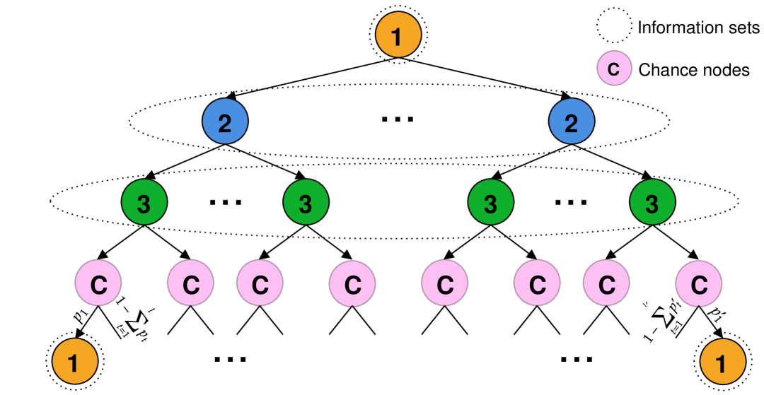
Figure 1: Extensive form of a three player SAA-c game with information sets and chance nodes

The standard representation for multi-round games is a tree representation named extensive form [18]. The game tree is a finite rooted directed tree admitting two types of nodes: decision nodes and chance nodes. At each decision node, a player has the choice between many actions represented each by a directed edge. A chance node has a fixed probabilistic distribution assigned over its outgoing edges. An information set is a set of decision nodes which are indistinguishable for the concerned player at the current position of the game [9]. This means that a player, given its current information, does not know exactly at which decision node it is playing. It only knows that it is playing at one of the decision nodes of the corresponding information set. Games where information sets are not all singletons are known as imperfect information games [24].

We represent the SAA-c game in this form with the decision nodes representing the different states of the game and the chance nodes representing the random draws of temporary winners in case of ties. At each decision node, an outgoing edge represents a set of items on which the concerned player bids if it selects this edge. Each decision node or state is defined by five features: the concerned player, the eligibility vector revealed at the end of the last round, the temporary winner of each item, the current bid price vector and the bids already submitted during the current round. The four first features are common knowledge and the last feature is hidden information for the concerned player. Therefore, all decision nodes which differ only by the last feature belong to the same information set. In Figure 1, we represent an SAA-c game between three players with their information sets and chance nodes.

II-D Game and strategical complexities

II-D1 Game complexities

To highlight the complexity of the SAA-c game, we focus on two metrics: information set space complexity and game tree complexity [28]. We define the first as the number of different information sets which can be legally reached in the game. It acts as a lower bound of the state space complexity [28]. The second corresponds to the number of different paths in its extensive form. We compute both complexities for a given number of rounds $R$, unlimited budgets and without any activity rule.

Theorem 2.1.

Let $\Gamma$ be an instance of the SAA-c game with no activity rule. Let $n$, $m$ and $R$ be respectively the number of players, the number of items and the number of rounds in $\Gamma$. Suppose that all players have unlimited budgets. The number of possible information sets in $\Gamma$ is:

$$n(Rn+1)^{m}$$ (3)

Proof.

Each information set is defined by three components: the player to bid, the temporary winner and bid price of each item. If no player has bidded on an item, then it remains unsold and is handed back to the auctioneer. Otherwise, its bid price is included in $\{\varepsilon,2\varepsilon,...,R\varepsilon\}$ and the item is allocated to one of the $n$ players. Therefore, the number of different allocations and bid prices of an item in $\Gamma$ is $Rn+1$. Under the unlimited budget assumption, all items are mutually independent. Thus, the number of different allocations and bid prices for all items is $(Rn+1)^{m}$. As there are $n$ different players who can bid, the number of possible information sets is:

$$n(Rn+1)^{m}$$

∎

Theorem 2.2.

Let $\Gamma$ be an instance of the SAA-c game with no activity rule. Let $n$, $m$ and $R$ be respectively the number of players, the number of items, and the number of rounds in $\Gamma$. Suppose that all players have unlimited budgets. A lower bound of the game tree complexity of $\Gamma$ is:

$$\Omega(2^{m(n-1)R})$$ (4)

Proof.

We consider $\Gamma$ with a deterministic tie-breaking rule. This eliminates chance nodes and reduces the number of paths in the game’s extensive form. Let’s first compute a lower bound of the number of different branches created in $\Gamma$ during a given round.

Suppose player $i$ is the temporary winner of $m_{i}$ items. Thus, during this given round, player $i$ can bid $2^{m-m_{i}}$ different ways as it can either bid or not bid on each of the remaining $m-m_{i}$ items. Hence, during this round, there are $2^{nm-\sum_{i=1}^{n}m_{i}}$ different bidding scenarios. Thus, this given round creates $2^{nm-\sum_{i=1}^{n}m_{i}}-1$ new branches all leading to non-terminal nodes of $\Gamma$. Moreover, as $\sum_{i=1}^{n}m_{i}\leq m$, the number of different branches created during any round is lower bounded by $2^{m(n-1)}-1$.

A lower bound of the game tree complexity of $\Gamma$ can then easily be calculated by induction. Indeed, every non-terminal node of $\Gamma$ starting a bidding round induces at least $2^{m(n-1)}-1$ new branches during this round. Therefore, the game tree complexity of $\Gamma$ is lower bounded by:

$$\sum_{l=0}^{R}(2^{m(n-1)}-1)^{l}=\frac{(2^{m(n-1)}-1)^{R+1}-1}{2^{m(n-1)}}$$ (5)

Thus, a lower bound of the game tree complexity of $\Gamma$ is $\Omega(2^{m(n-1)R})$. ∎

Example.

An SAA for 12 spectrum licences (5G) between 5 telecommunication companies was held in Italy in 2018 and ended after 171 rounds [12]. The number of possible information sets as well as a lower bound of the game tree complexity of the corresponding SAA-c game with no activity rule are respectively $10^{35}$ and $10^{2470}$.

Adding activity rules decreases the game tree complexity as a bidder can no longer bid on a set of items which exceeds its eligibility. However, it increases the information set space complexity as a new feature (eligibility) is added to every information set.

II-D2 Strategical complexities

SAA-c game also admits a number of strategical issues. The four main ones are presented below.

• Exposure: It is a phenomenon which happens when a player tries to acquire a set of complementary items but ends up by paying too much for the subset it actually wins at the end of the auction. Hence, the player obtains a negative utility. For instance, Table I presents a well-studied example, see e.g. [30], in a 2-item SAA-c game with a bid increment of $1$ between two players with unlimited budgets (referred to as Example 1). Player 1 considers both items as perfect substitutes, i.e. it values both items equally and desires to acquire only one of the two, while player 2 considers them as perfect complements, i.e. each item is worthless without the other and desires to acquire both of them. If player 1 is temporarily winning no items and the bid price of the cheapest item is lower than $11$, it should bid on it. Otherwise, it should pass. Hence, if player 2 decides to bid on both items, it will end up exposed as it won’t be able to obtain both items for a price inferior to 22. Moreover, if after a few rounds, player 2 decides to give up an item, it will still end up by paying for the other item and, hence, incur a loss.

  TABLE I: Example of exposure ($\varepsilon=1$)

  	$v(\{1\})$	$v(\{2\})$	$v(\{1,2\})$
  Player 1	12	12	12
  Player 2	0	0	20

• Own price effect: Competing on an item causes inevitably the rise of its bid price and, hence, the decrease in utility of all players wishing to acquire it. Thus, players have all a strong interest in maintaining the bid price of all items as low as possible. To avoid this rise, a player can concede items to its opponents hoping that they will not bid on the items it is temporarily winning in exchange. This strategy is known as demand reduction [29, 3]. Dividing items between players to avoid this issue is called collusion [5]. No communication is allowed between players. In SAA-c, players should be able to use the common knowledge of valuations and budgets to agree on a same fair split of items to tackle this issue without any communication.

• Budget constraints: Capping the maximum amount a bidder can spend during an auction can highly impact the auction’s outcome. Indeed, it can prevent players from bidding on certain sets of items and be a source of exposure. Moreover, given this information, players can drastically change their bidding strategy. For instance, in the auction presented in Table I, if player 1 and 2 have respectively a fixed budget of $8$ and $20$, player 2 should bid on both items as this situation no longer presents any risk of exposure.

• Eligibility management: Managing efficiently its own eligibility is essential to ensure a favourable outcome. Bidding on a high number of items to maintain high eligibility induces the own price effect. However, reducing its eligibility to form collusions can trap a bidder in a vulnerable position if the other bidders do not behave as expected. Hence, a tradeoff must be found.

II-E Performance indicators

The natural metric used to measure the performance of a strategy is the expected utility. However, given the fact that a specific instance of a spectrum auction (i.e. same frequency bands, same operators, etc …) is generally only held once and an operator just participates to a few different instances, comparing strategies only on the basis of their expected utility is not sufficient. Indeed, given the huge amount of money involved, potential losses due to exposure should also be taken into account. To measure this risk, we decompose the expected utility as follows:

$$\begin{split}\operatorname{\mathbb{E}}(R^{\pi})=\text{I\kern-1.49994ptP}(R^{\pi}\geq 0)\operatorname{\mathbb{E}}(R^{\pi}|R^{\pi}\geq 0)+\underbrace{\text{I\kern-1.49994ptP}(R^{\pi}\textless 0)\operatorname{\mathbb{E}}(R^{\pi}|R^{\pi}\textless 0)}_{\text{Exposure}}\end{split}$$ (6)

where $\pi$ is a policy and $R^{\pi}$ is a random reward obtained by playing $\pi$ in a SAA-c game. We introduce the term $-\text{I\kern-1.49994ptP}(R^{\pi}\textless 0)\operatorname{\mathbb{E}}(R^{\pi}|R^{\pi}\textless 0)$ as a metric of potential exposure which should be minimised. We name it expected exposure and estimate it by taking the opposite of all losses incurred by a strategy divided by the number of plays. Moreover, we define the exposure frequency as $\text{I\kern-1.49994ptP}(R^{\pi}\textless 0)$. This is estimated by the number of times a strategy incurs a loss divided by the number of plays. To analyse the own price effect, we consider the average price payed per item won. However, by only acquiring undesired items at reasonably low price, a bidder can obtain a low average price payed per item won. Hence, we complement this metric by the ratio of items won.

III Predicting closing prices

$SMS^{\alpha}$ is based on a SM-MCTS whose expansion and rollout phases rely on the following bidding strategy and prediction of closing prices, i.e., an estimation of the price of each item at the end of the auction.

III-A Constrained point-price prediction bidding

We start by extending the definition of point-price prediction bidding (PP) [30] to budget and eligibility constrained environments.

Definition 3.1.

In a SAA-c game with $m$ objects and a current bid price vector $P$, a point-price prediction bidder with budget $b$, a current eligibility $e$, an initial prediction of closing prices $P^{init}$ and a set of temporarily won items $Y$ computes the subset of goods

$$X^{*}=\underset{\begin{subarray}{c}X\subset\{\emptyset\}\cup\{1,...,m\}\backslash Y\\ \sum_{j\in X\cup Y}\rho_{j}(P^{init},P,Y)\leq b\\ |X|+|Y|\leq e\end{subarray}}{\text{arg max}}\;\sigma(X\cup Y,\rho(P^{init},P,Y))$$ (7)

breaking ties in favour of smaller subsets and lower-numbered goods. It then bids $P_{j}+\varepsilon$ on all items $j$ belonging to $X^{*}$. The function $\rho:(P^{init},P,Y)\rightarrow\mathbb{R_{+}}^{m}$ maps an initial prediction of closing prices, a current bid price vector and a set of items temporarily won to an estimation of closing prices. For any item $j$, it follows the below update rule:

$$\rho_{j}(P^{init},P,Y)=\left\{\begin{array}[]{ll}\max(P^{init}_{j},P_{j})&\text{if }j\in Y\\ \max(P^{init}_{j},P_{j}+\varepsilon)&\text{otherwise}\\ \end{array}\right.$$ (8)

A point-price prediction bidder only considers sets of items within budget $b$ given its prediction of closing prices $\rho(P^{init},P,Y)$, i.e., only sets of items $X$ such that $\sum_{j\in X\cup Y}\rho_{j}(P^{init},P,Y)\leq b$. Moreover, it can only bid on sets of items which does not exceed its eligibility $e$.

If closing prices are correctly estimated and independent of the bidding strategy, then playing PP is optimal for a player. However, in practice, closing prices are usually tightly related to a player’s bidding strategy. Playing PP with a null prediction of closing prices ($P^{init}=0$) is known as straightforward bidding (SB) [19]. The efficiency of the bidding strategy PP highly depends on the accuracy of the initial prediction of closing prices $P^{init}$. For instance, if $P^{init}$ largely underestimates the actual closing price of each item, then when the current bid price $P\geq P^{init}$ component-wise, playing PP with initial prediction $P^{init}$ gives the same strategy as SB. However, if $P^{init}$ overestimates too much the actual closing price of each item, then the bidder might stop playing prematurely in order to avoid exposure.

III-B Computing an initial prediction of closing prices

Several methods exist in the literature for computing an initial prediction of closing prices $P^{init}$ in budget constrained environments. However, they all seem to present some limitations in SAA-c. For instance, the well known Walrasian price equilibrium [2] do not always exist when preferences exhibit complementarities as it is the case in Example 1. Standard tâtonnement processes, such as the one used to compute expected price equilibrium [30], return the same price vector regardless of the auction’s specificities (e.g., bid increment $\varepsilon$). The final prediction is then completely independent of the auction mechanism of SAA-c which is problematic. Computing an initial prediction by using only the outcomes of a single strategy profile is relevant only if bidders actually play according to this strategy profile. For instance, simulating SAA-c games where all bidders play SB and using the average closing prices as initial prediction is relevant if the actual bidders play SB. We propose hereafter a prediction method based on the convergence of a specific sequence which aims at tackling all of these issues.

Conjecture 3.1.

Let $\Gamma$ be an instance of an SAA-c game. Let $f_{\Gamma}(P)$ be a random variable returning the closing prices of $\Gamma$ when all bidders play PP with initial prediction $P$. The sequence $p_{t+1}=\frac{1}{t+1}\operatorname{\mathbb{E}}[f_{\Gamma}(p_{t})]+(1-\frac{1}{t+1})p_{t}$ with $p_{0}$ the null vector of prices converges to a unique element $p^{*}$.

The fact that $f_{\Gamma}$ is a random variable comes from the tie-breaking rule which introduces stochasticity in $\Gamma$. By taking its expectation $\operatorname{\mathbb{E}}[f_{\Gamma}(p_{t})]$ at each iteration $t$, we ensure our deterministic sequence $p_{t}$ to always converge to the same fixed point $p^{*}$. Hence, all players using our method share the same prediction of closing prices $p^{*}$. In practice, we perform a Monte-Carlo estimation of $\operatorname{\mathbb{E}}[f_{\Gamma}(p_{t})]$ by simulating many SAA-c games. In small instances, it is possible to obtain a closed-form expression of $\operatorname{\mathbb{E}}[f_{\Gamma}(p_{t})]$ and, from that, prove the convergence of sequence $p_{t}$.

Example.

Suppose that both players play PP with $P^{init}=p_{0}$ in Example 1. During the first round, player 1 bids on item 1 and player 2 bids on both items. There is $50\%$ chance that player 1 temporarily wins item 1 and $50\%$ chance that player 2 temporarily wins item 1. If player 1 wins item 1 during the first round, player 2 bids on item 1 during the second round while player 1 passes. In the third round, player 1 bids on item 2 while player 2 passes. In the fourth round, player 2 bids on item 2 while player 1 passes. Hence, the bid price of item 1 (respectively item 2) is odd (respectively even) if temporarily won by player 1. When the bid price $P=(12,11)$ and both items are temporarily won by player 2, player 1 drops out of the auction as, by definition of PP, it prefers smaller subsets of items for a same predicted utility. If player 2 wins item 1 during the first round, the bid price of item 1 (respectively item 2) is even (respectively even) if temporarily won by player 1. The closing price are then $P=(11,11)$. Therefore, $f_{\Gamma}(p_{0})$ has 50% chance of returning $(12,11)$ and 50% chance of returning $(11,11)$. Hence, $\operatorname{\mathbb{E}}[f_{\Gamma}(p_{0})]=(11.5,11)$. By performing a similar analysis, we can show that $\forall p\in\mathbb{R}^{2},\operatorname{\mathbb{E}}[f_{\Gamma}(p)]\in[0,11.5]^{2}$ and obtain the following closed-form expression for any $p\in[0,11.5]^{2}$:

$${\operatorname{\mathbb{E}}[f_{\Gamma}}(p)]=\left\{\begin{array}[]{ll}(1,0)&\text{if }p_{1}+p_{2}\geq 20\text{ and }p_{1}\leq p_{2}\\ (0,1)&\text{if }p_{1}+p_{2}\geq 20\text{ and }p_{1}>p_{2}\\ (11.5,11)&\text{if }p_{1}+p_{2}<20\text{ and }p_{1}\leq p_{2}\\ (11,11.5)&\text{if }p_{1}+p_{2}<20\text{ and }p_{1}>p_{2}\\ \end{array}\right.$$ (9)

From there, it is easy to show that sequence $p_{t}$ converges to $p^{*}=(10,10)$ in Example 1.

The general proof of the conjecture is left for future work.

Computing an initial prediction of closing prices as above has mainly three advantages compared to other methods in the literature. (1) We observe that this sequence converges in all undertaken SAA-c game instances. (2) This method takes into account the auction’s mechanism through $f_{\Gamma}$. (3) This prediction of closing price is not based only on the outcomes of a single specific strategy profile. Indeed, depending on the value of $p_{t}$, different strategy profiles are used across iterations. At a fixed iteration $t$, a single strategy profile is used to compute $\operatorname{\mathbb{E}}[f_{\Gamma}(p_{t})]$ as the strategy returned by PP only depends on its initial prediction $P^{init}=p_{t}$.

IV SM-MCTS bidding strategy

IV-A Brief presentation of MCTS

Given the large state space and game tree complexities, it is practically impossible to explore the SAA-c game tree exhaustively as soon as we depart from very small instances. Thus, only a small portion of the game tree, called the search tree, can be explored. MCTS is a search technique that builds iteratively a search tree using simulations through a process named search iteration (see Figure 2). Each search iteration is divided into four steps. (1) The selection phase selects a path from the root to a leaf node of the search tree. (2) The expansion phase chooses one or more children to be added to the search tree from the selected leaf node according to the available actions. (3) The simulation phase simulates the outcome of the game from the newly added node. (4) The backpropagation phase propagates backwards the outcome of the game from the newly added node to the root in order to update the diverse statistics stored in each selected node of the search tree. This process is repeated until some predefined computational budget (time, memory, iteration constraint) is reached. Before running $SMS^{\alpha}$, we compute our initial prediction of closing prices $p^{*}$ as presented in Section III-B.

Figure 2: MCTS scheme

IV-B Scalarised rewards

Maximising the expected utility while minimising the risk of exposure can be antithetical. Indeed, taking risks can either be highly beneficial or lead to exposure depending on how the other players react. To do so, we introduce a new scalarised reward incorporating both targets. For any strategy $\pi$, we define:

$$R_{\alpha}^{\pi}=(1+\alpha\mathbb{1}_{R^{\pi}<0})R^{\pi}$$ (10)

where $\alpha$ is a hyperparameter which controls the risk aversion of $SMS^{\alpha}$. Note that

$$\operatorname{\mathbb{E}}(R_{\alpha}^{\pi})=\operatorname{\mathbb{E}}(R^{\pi})+\alpha\text{I\kern-1.49994ptP}(R^{\pi}\textless 0)\operatorname{\mathbb{E}}(R^{\pi}|R^{\pi}\textless 0)$$ (11)

where $\text{I\kern-1.49994ptP}(R^{\pi}\textless 0)\operatorname{\mathbb{E}}(R^{\pi}|R^{\pi}\textless 0)$ is the term corresponding to the losses induced by exposure in Equation 6. Moreover, we define for any vector of price $P$ and any set of items $X$, $\sigma^{\alpha}(X,P)=(1+\alpha\mathbb{1}_{\sigma(X,P)<0})\sigma(X,P)$ which is a modified utility taking into account both of our objectives.

The use of a linear scalarization function is a classical approach in multi-objective optimisation, multi-objective reinforcement learning [4], constrained MDP [15] or POMDP [16].

IV-C Search tree structure

In order to maintain the simultaneous nature of SAA-c in the selection phase of $SMS^{\alpha}$, we use a Simultaneous Move MCTS (SM-MCTS) [27] (Figure 3). At each selection step, we select an $n$-tuple where each index $i$ corresponds to the action maximising the selection index of player $i$ given only its information set. By doing so, bids are selected simultaneously and independently. Each selection step corresponds to a complete bidding round of SAA-c. Hence, the depth of our search tree corresponds to how many rounds ahead $SMS^{\alpha}$ can foresee. The search tree nodes are defined by the eligibility of each bidder, the temporary winner and current bid price of each item. The vertices correspond to players’ joint actions. Chance nodes are explicitly included in the search tree to break ties. The main advantage of SM-MCTS compared to applying MCTS on a serialised game tree, i.e. turning SAA-c into a purely sequential game, is that, to complete a bidding round of SAA-c, the number of selection steps is reduced from $n$ to $1$. Hence, by using SM-MCTS, the number of players $n$ is no longer a burden for planning a bidding strategy over many rounds. Moreover, statistics are stored per information set and no longer per state which reduces memory consumption.

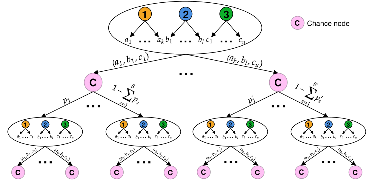
Figure 3: SM-MCTS tree structure with explicit chance nodes for SAA-c game with 3 players

IV-D Selection

At each selection step, players are asked to bid on the set of items which maximises their selection index. The selection phases ends when a terminal state of the SAA-c game or a non-expanded node, i.e. configuration of temporal winners, bid prices and eligibilities not yet added to the search tree, is reached. Our selection index is a direct application of the Upper Confidence bound applied to Trees (UCT) [14] to scalarised rewards. Unlike usual applications of UCT, the size of the scalarised reward support is unknown so we proceed to an online estimation of it. Each player $i$ chooses to bid on the set of items $x_{i}$ with highest score $q_{x_{i}}$ at information set $I_{i}$:

$$\begin{split}q_{x_{i}}=\frac{r^{\alpha}_{x_{i}}}{n_{x_{i}}}+\max(c^{\alpha}_{x_{i}}-a^{\alpha}_{x_{i}},\varepsilon)\sqrt{\frac{2\log(\sum_{x^{\prime}_{i}}n_{x^{\prime}_{i}})}{n_{x_{i}}}}\end{split}$$ (12)

where $r^{\alpha}_{x_{i}}$ is the sum of scalarised rewards obtained after bidding on $x_{i}$ at $I_{i}$, $n_{x_{i}}$ is the number of times player $i$ has bidded on $x_{i}$ at $I_{i}$, $\varepsilon$ is the bid increment, $a^{\alpha}_{x_{i}}$ is the estimated lower bound and $c^{\alpha}_{x_{i}}$ is the estimated higher bound of the scalarised reward support when bidding on $x_{i}$ at $I_{i}$. Thus, $\max(c^{\alpha}_{x_{i}}-a^{\alpha}_{x_{i}},\varepsilon)$ acts like the size of scalarised reward support when bidding on $x_{i}$ at $I_{i}$.

IV-E Expansion

The high branching factor due to the exponential growth of the game tree’s width with the number of items $m$ prevents in-depth inspection of promising branches. Thus, it is necessary to reduce the action space at each information set of the search tree [24]. To do so, each time a non-expanded node is added to the search tree, we select a maximum number $N_{act}$ of promising actions per information set. Passing its turn without bidding on any item is always included in the $N_{act}$ selected actions. This enables $SMS^{\alpha}$ to obtain shallow terminal nodes in its search tree which correspond to collusions between bidders and, thus, reduces the own price effect. The remaining $N_{act}-1$ actions correspond to the moves leading to the $N_{act}-1$ highest predicted utilities in strategy PP with initial prediction $p^{*}$. More formally, for each player $i$ at information set $I_{i}$ temporarily winning set of items $Y_{i}$ with eligibility $e_{i}$, the action of bidding on set of items $X_{i}$ is selected if $\sigma_{i}^{\alpha}(Y_{i}\cup X_{i},\rho(p^{*},P,Y_{i}))$ is one of the $N_{act}-1$ highest values with $P$ the current bid price. Only sets of items $X_{i}$ verifying $\sum_{j\in X_{i}\cup Y_{i}}\rho_{j}(p^{*},P,Y_{i})\leq b_{i}$ and $|X_{i}|+|Y_{i}|\leq e_{i}$ are considered. Statistics for each action are then initialised as follows:

• $r^{\alpha}_{x_{i}}\leftarrow 0$

• $n_{x_{i}}\leftarrow 0$

• $a^{\alpha}_{x_{i}}\leftarrow+\infty$

• $c^{\alpha}_{x_{i}}\leftarrow-\infty$

IV-F Rollout

From the newly added node, an SAA-c game is simulated until the game ends. Players are asked to bid at each round of the rollout. The default strategy is usually to bid on a random set of items. However, it leads to absurd outcomes in this case with very high prices as player rarely all pass. Therefore, we propose an alternative approach. At the beginning of each rollout phase, we set $p^{*}_{i}=p^{*}+\eta_{i}$ with $\eta_{i}\sim U([-\varepsilon,\varepsilon]^{m})$. Each player $i$ then plays PP with initial prediction of closing prices $p^{*}_{i}$ during the entire rollout. Noise is added to our initial prediction $p^{*}$ to diversify players’ bidding strategy and, hence, improve the quality of our sampling. At the end of the rollout, an $n$-tuple is returned corresponding to the scalarised utility obtained by each player.

IV-G Backpropagation

The results obtained during the rollout phase are propagated backwards to update the statistics of the selected nodes. Let $V^{\alpha}_{i}$ be the scalarised utility obtained by player $i$ at the end of the rollout. Let $x_{i}$ be the set of items on which player $i$ bidded at information state $I_{i}$ for one of the selected nodes. The statistics stored for $I_{i}$ are updated as follows:

• $r^{\alpha}_{x_{i}}\leftarrow r^{\alpha}_{x_{i}}+V^{\alpha}_{i}$

• $n_{x_{i}}\leftarrow n_{x_{i}}+1$

• $a^{\alpha}_{x_{i}}\leftarrow\min(a^{\alpha}_{x_{i}},V^{\alpha}_{i})$

• $c^{\alpha}_{x_{i}}\leftarrow\max(c^{\alpha}_{x_{i}},V^{\alpha}_{i})$

IV-H Transposition table

Transposition tables are a common search enhancement used to considerably reduce the size of the search tree and improve performance of MCTS within the same computational budget [8]. By using such tables, we prevent the expansion of redundant nodes in our search tree and share the same statistics between transposed information states. This results in a significant improvement in performance of $SMS^{\alpha}$ for a same amount of thinking time.

To identify each information set in the search tree, our hash function is based on two functions $h_{1}$ and $h_{2}$. The first returns a different integer for each combination of bid prices and allocations. The second returns a different integer for each eligibility vector. Hence, our hash function assigns a unique value to each information set in the search tree. More precisely, due to computational constraints, we can only assign a unique value for every node in the search tree with a depth lower than $R_{max}$. $R_{max}$ is a hyperparameter corresponding to an upper bound of the maximal depth (or rounds) in the final search tree. An example of function $h_{1}$ assigning a different integer for each combination of bid prices and allocations in a search tree of maximal depth $R_{max}$ is given in Algorithm 1. It uses as inputs the bid price vector $P^{0}$ at the root of the search tree, the bid price vector $P$ and the temporary winner $A_{j}$ of each item $j$ at a given node. If $A_{j}=0$, then item $j$ is temporarily allocated to the auctioneer.

In practice, given the thinking time constraints in our experimental results, choosing $R_{max}=10$ is more than sufficient to guarantee a final search tree with maximal depth lower than $R_{max}$. Hence, our hash function acts as a perfect hash function as no type-1 error or type-2 error occurs [32].

Algorithm 1 Example of function $h_{1}$

Inputs Game: $n$, $m$, $\varepsilon$

Inputs Root Node: Bid price vector $P^{0}$

Inputs Node: Bid price vector $P$, Allocation vector $A$

Hyperparameter: $R_{max}$

$h=0$

$step=R_{max}\times n$

for $j=1,2,...,m$ do

     if $A_{j}>0$ then $h+=(R_{max}\times(A_{j}-1)+\frac{P_{j}-P^{0}_{j}}{\varepsilon})step^{j-1}$

     end if

end for

return h

IV-I Final move selection

The final move which is returned by $SMS^{\alpha}$ is the action which maximises the player’s expected scalarised reward at the root node. More formally, $SMS^{\alpha}$ returns $\underset{x_{i}}{\text{arg max}}\frac{r_{x_{i}}^{\alpha}}{n_{x_{i}}}$ for player $i$.

V Experiments

In this section, we start by analysing the convergence rates of sequence $p_{t}$, notably through Example 1. Then, we show that our algorithm $SMS^{\alpha}$ largely outperforms state-of-the-art existing bidding algorithms in SAA-c, mainly by tackling own price effect and exposure more efficiently. This is first shown through typical examples taken from the literature and, then, through extensive experiments on instances of realistic size. We compare $SMS^{\alpha}$ to the following four strategies:

• $MS^{\lambda}$: An MCTS algorithm described in [22] which relies on two risk-aversion hyperparameters $\lambda^{r}$ and $\lambda^{o}$.

• EPE: A PP strategy using expected price equilibrium [30] as initial prediction.

• SCPD: A distribution price prediction strategy using self-confirming price distribution [30] as initial distribution prediction.

• SB: Straightforward bidding [19].

The four strategies $MS^{\lambda}$, EPE, SCPD and SB initially rely on the definition of PP for unconstrained environments [30]. We extend them to budget and eligibility constrained environments in the same way as it is done in Definition 3.1. In all experiments, none of the bidders are aware of their opponents’ strategy.

Each algorithm is given respectively $150$ seconds of thinking time. Initial prediction of closing prices are done offline before the auction starts and, therefore, are excluded from the thinking time. This step usually takes a few minutes. All experiments are run on a server consisting of Intel®Xeon®E5-2699 v4 2.2GHz processors. In all upcoming experiments, the hyperparameter $\alpha$ of $SMS^{\alpha}$ takes the value $7$ and the risk-aversion hyperparameters $\lambda^{r}$ and $\lambda^{o}$ of $MS^{\lambda}$ both take the value $0.025$. These hyperparameters are obtained by grid-search. The maximum number of expanded actions per information set $N_{act}$ of $SMS^{\alpha}$ is set to $20$.

V-A Convergence of sequence $p_{t}$

One of the main advantages of using our method to compute an initial prediction is the convergence of sequence $p_{t}$. Even though this convergence has only been observed and not proven, it is possible to derive rates of convergence in small instances. For instance, in Example 1, it can be shown that $\forall t\geq 1$, $p_{t}$ belongs to the diamond defined by the points $(10-\frac{10}{t},10-\frac{9}{t})$, $(10-\frac{9}{t},10-\frac{10}{t})$, $(10+\frac{7}{4t},10+\frac{3}{4t})$ and $(10+\frac{3}{4t},10+\frac{7}{4t})$ which converges to $p^{*}=(10,10)$. We represent in Figure 4 the sequence $p_{t}^{1}$ with its corresponding lower bound and upper bound.

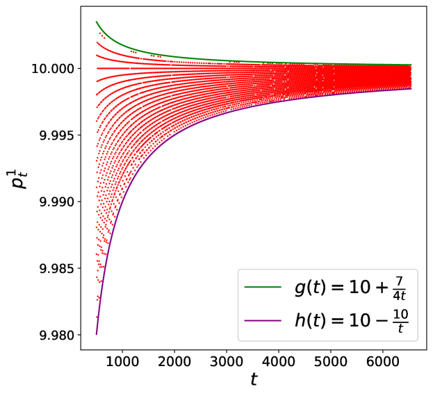
Figure 4: Convergence of sequence $p_{t}^{1}$ with its respective upper bound $g(t)$ and lower bound $h(t)$ in Example 1.

In larger instances, we observe similar rates of convergence. However, computing such bounds seems unrealistic as obtaining a closed-form expression of $\operatorname{\mathbb{E}}[f_{\Gamma}(p_{t})]$ seems untractable.

V-B Test experiments

One of the greatest advantages that MCTS methods have over other bidding algorithms is the capacity to judge pertinently in which situations adopting a demand reduction strategy is more beneficial. Indeed, through the use of its search tree, an MCTS method is capable of determining if it is more profitable to concede items to its opponents to keep prices low or to bid greedily. To highlight this feature, we propose the following experiment in a 2-item auction between two players with additive value functions. Each player values each item at $l=10$. Player 1 has a budget $b_{1}\geq 20$. Given that, the optimal strategy for player 2 is to bid on the cheapest item if it is not temporarily winning any item. Otherwise, it should pass. The optimal strategy for player 1 fully depends on its opponent’s budget $b_{2}$. For an infinitesimal bid increment $\varepsilon$,

• If $b_{2}\leq\frac{l}{2}$, player 1’s optimal strategy is to play straightforwardly and it obtains an expected utility of $l-2b_{2}$.

• If $b_{2}\geq\frac{l}{2}$, player 1’s should adopt a demand reduction strategy and it obtains an expected utility of $l$.

We plot in Figure 5 the expected utility $\operatorname{\mathbb{E}}(\sigma_{1})$ of player 1 for each strategy given player 2’s budget $b_{2}$. The three algorithms SB, EPE, SCPD always suggest to player 1 to bid greedily and never propose a demand reduction strategy even when it is highly profitable ($b_{2}>\frac{l}{2}$). However, both MCTS methods perfectly adopt the appropriate strategy. This experiment highlights the fact that $SMS^{\alpha}$ selects the most profitable strategy and tackles own price effect, at least in simple budget and eligibility constrained environments.

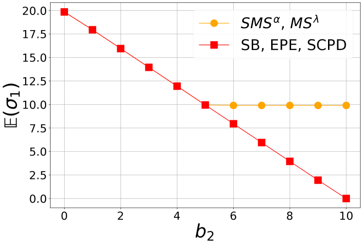
Figure 5: Evolution of player 1’s expected utility $\operatorname{\mathbb{E}}(\sigma_{1})$ depending on strategy versus player 2’s budget $b_{2}$ given that player 2 plays optimally ($\varepsilon=0.1$).

Furthermore, $SMS^{\alpha}$ is capable of avoiding obvious exposure. To highlight this feature, we use the SAA-c game presented in Example 1 where player 2’s budget $b_{2}=16$. The optimal strategy for player 1 is to play straightforwardly. Similarly to the preceding experiment, the optimal strategy for player 2 fully depends on its opponent’s budget $b_{1}$.

• If $b_{1}<8$, player 2’s optimal strategy is to play straightforwardly.

• If $b_{1}\geq 8$, player 2’s optimal strategy is to drop out of the auction to avoid exposure.

We plot in Figure 6 the expected utility $\operatorname{\mathbb{E}}(\sigma_{2})$ of player 2 for each strategy given player 1’s budget $b_{1}$. The two algorithms SCPD and SB always suggest to player 2 to bid straightforwardly leading player 2 to exposure when $b_{1}\geq 8$. $MS^{\lambda}$ never leads player 2 to exposure. However, it suggests to drop out prematurely of the auction in some situations with no risk of exposure and, hence, incurs a loss of easy profit ($b_{1}=7$). $SMS^{\alpha}$ and $EPE$ perfectly adopt the optimal strategy. This experiment highlights the fact that $SMS^{\alpha}$ perfectly adopts the most profitable strategy and tackles efficiently exposure, at least in simple budget and eligibility constrained environments.

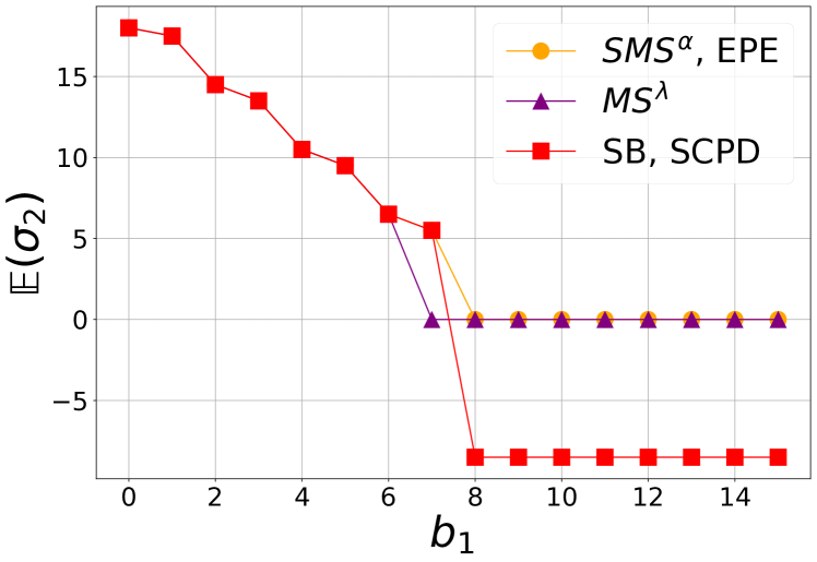
Figure 6: Evolution of player 2’s expected utility $\operatorname{\mathbb{E}}(\sigma_{2})$ depending on strategy versus player 1’s budget $b_{1}$ given that player 1 plays optimally in Example 1 ($\varepsilon=1$).

V-C Extensive experiments

In this section, we study instances of realistic size with $n=4$ and $m=11$. Each experimental result has been run on 1000 different SAA-c instances. With the exception of [22], all experimental results in the literature are obtained for specific settings of SAA, i.e., using value functions with some specific property such as superadditivity [13, 30, 23]. Hence, it is difficult to conclude on the effectiveness of a method in more generic settings. Therefore, we propose a more general approach to generate value functions by making no additional assumption on its form. Budgets are drawn randomly.

Setting.

Let $\Gamma$ be an instance of SAA-c with $n$ bidders, $m$ items and bid increment $\varepsilon$. Each player $i$ has a budget $b_{i}\sim U([b_{min},b_{max}])$ with $U$ the uniform distribution. Its value function $v_{i}$ is built as follows: $v_{i}(\emptyset)=0$ and, for any set of goods $X$,

$$v_{i}(X)\sim U([\max_{j\in X}v_{i}(X\backslash\{j\}),V+\max_{j\in X}v_{i}(X\backslash\{j\})+v_{i}(\{j\})])$$ (13)

Drawing value functions through a uniform distribution is widely used for creating auction instances [30, 23]. In our setting, the lower-bound ensures that $v_{i}$ respects the free disposal [19] condition. The upper-bound caps the maximum surplus of complementarity possibly gained by adding an item $j$ to the set of goods $X\backslash\{j\}$ by $V$. As valuations are always finite, any value function can be represented by our setting for a sufficiently large $V$. For $V=0$, only subadditive functions are considered. For $V>0$, goods can either be complements or substitutes. In our experimental results, value functions and budgets are generated for each instance as above with $\varepsilon=1$, $b_{min}=10$, $b_{max}=40$ and $V=5$.

In the upcoming analysis, the average price payed per item won, the ratio of items won, the expected exposure and the exposure frequency are obtained by confronting a strategy $A$ to a strategy $B$. To facilitate our study, each measure of $A$ against $B$ is obtained by averaging the results obtained for the three following strategy profiles: ($A$,$B$,$B$,$B$), ($A$,$A$,$B$,$B$) and ($A$,$A$,$A$,$B$). For instance, if $A=SMS^{\alpha}$ and $B=\text{SB}$, the average price payed per item won by $SMS^{\alpha}$ in these three strategy profiles is respectively: $5.96$, $5.46$ and $4.62$. Hence, the average price payer per item won by $SMS^{\alpha}$ against $SB$ is $5.35$.

V-C1 Expected Utility

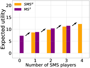
(a) $SMS^{\alpha}$ vs $MS^{\lambda}$

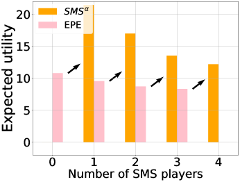
(b) $SMS^{\alpha}$ vs EPE

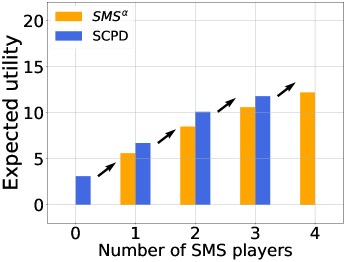
(c) $SMS^{\alpha}$ vs SCPD

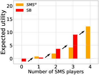
(d) $SMS^{\alpha}$ vs SB

Figure 7: Normal-form expected utility for a SAA-c game with five strategies

To facilitate our analysis, we study the normal form game in expected utility where each player has the choice between playing $SMS^{\alpha}$ or another strategy $A$. The same empirical game analysis approach was employed by Wellman et al. in [30]. More precisely, we map each strategy profile to the estimated expected utility obtained by each player in the 1000 SAA-c instances. The four resulting empirical games for each possible strategy $A$ are given in Figure 7.

For example, in Figure 7b, if all bidders play EPE, each bidder obtains an expected utility of $10.8$. In the case of three EPE bidders and one $SMS^{\alpha}$ bidder, the $SMS^{\alpha}$ bidder obtains an expected utility of $21.5$. Hence, if all bidders play EPE, a bidder can double its expected utility by switching to $SMS^{\alpha}$. Therefore, deviating to $SMS^{\alpha}$ is profitable if all bidders play EPE. This is also the case for the three other possible deviations in Figure 7b. Hence, in the empirical game where bidders have the choice between playing $SMS^{\alpha}$ or EPE, each bidder has interest in playing $SMS^{\alpha}$. We can clearly see that all deviations to $SMS^{\alpha}$ are also strictly profitable in the three other empirical games. Hence, in each empirical game, a bidder should play $SMS^{\alpha}$ to maximise its expected utility. Therefore, the strategy profile ($SMS^{\alpha}$, $SMS^{\alpha}$, $SMS^{\alpha}$, $SMS^{\alpha}$) is a Nash equilibrium of the normal-form SAA-c game in expected utility with strategy set {$SMS^{\alpha}$, $MS^{\lambda}$, EPE, SCPD, SB}.

Moreover, the strategy profile where all bidders play $SMS^{\alpha}$ has a significantly higher expected utility than any other strategy profile where all bidders play the same strategy. This is mainly due to the fact that $SMS^{\alpha}$ tackles efficiently the own price effect. For instance, in Figure 7, the expected utility of the strategy profile where all bidders play $SMS^{\alpha}$ is respectively $1.13$, $1.68$ and $3.94$ times higher than the ones where all bidders play EPE, $MS^{\lambda}$ and SCPD.

The fact that the expected utility obtained by the strategy profile where all bidders play EPE is relatively close to the one where all bidders play $SMS^{\alpha}$ can be explained as follows. To compute their expected price equilibrium as initial prediction of closing prices, all EPE bidders in our experiments share the same initial price vector and adjustment parameter in their tâtonnement process. This tâtonnement process is independent of the auction’s mechanism and only relies on the estimated valuations of the players. Hence, as SAA-c is a game with complete information, all EPE bidders share the same initial prediction of closing prices and can therefore split up the items between them more or less efficiently.

Not all algorithms have the ability of achieving good coordination between bidders. For instance, the strategy profile where all bidders play SB leads to a negative expected utility. Hence, in this specific case, bidders would have preferred not to participate in the auction. This highlights the fact that playing SB is a very risky strategy and mainly leads to exposure.

The high performance of $SMS^{\alpha}$ is mostly due to the three following factors:

• its ability to judge if performing demand reduction or bidding greedily is more beneficial given each bidder’s budget and eligibility.

• its ability to tackle the own price effect without putting itself in a vulnerable position because of eligibility constraints.

• its ability to avoid exposure in a budget and eligibility constrained environment.

V-C2 Own Price Effect

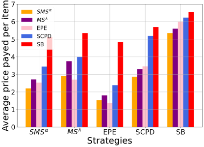
(a) Average price per item won

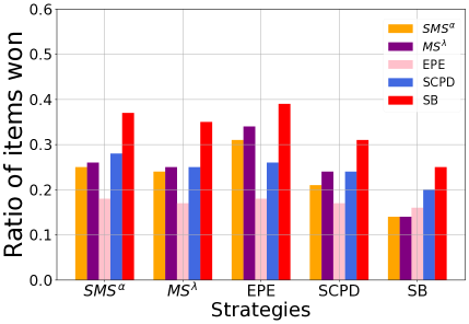
(b) Ratio items won

Figure 8: Own price effect analysis for a SAA-c game with five strategies

To analyse own price effect, we plot in Figure 8a the average price payed per item won by each strategy $A$ against every strategy $B$ displayed on the x-axis. For instance, if $A=SMS^{\alpha}$ and $B=\text{EPE}$, the average price payed per item won by $SMS^{\alpha}$ against EPE is $1.53$. It corresponds to the orange bar above index EPE on the x-axis. If $A=\text{EPE}$ and $B=SMS^{\alpha}$, then the average price payed per item won by EPE against $SMS^{\alpha}$ is $2.53$. It corresponds to the pink bar above index $SMS^{\alpha}$ on the x-axis.

In Figure 8a, we can clearly see that $SMS^{\alpha}$ acquires items at a lower price in average than the other strategies against $SMS^{\alpha}$, SCPD and SB. For instance, $SMS^{\alpha}$ spends $13.3\%$, $17.1\%$, $44.9\%$ and $49.8\%$ less per item won against SCPD than $MS^{\lambda}$, EPE, SCPD and SB respectively. Moreover, against $MS^{\lambda}$ and EPE, only EPE spends slightly less than $SMS^{\alpha}$ per item won.

To ensure that $SMS^{\alpha}$ bidders do not obtain low average prices by only purchasing undesired items, we plot in Figure 8b the ratio of items won by playing each strategy $A$ against every strategy $B$ on the x-axis. For instance, if $A=SMS^{\alpha}$ and $B=\text{EPE}$, the ratio of items won by $SMS^{\alpha}$ against EPE is $0.31$. It corresponds to the orange bar above index EPE on the x-axis in Figure 8b. If $A=\text{EPE}$ and $B=SMS^{\alpha}$, the ratio of items won by EPE against $SMS^{\alpha}$ is $0.18$. It corresponds to the pink bar above index $SMS^{\alpha}$ on the x-axis in Figure 8b. We see that each $SMS^{\alpha}$ bidder obtains at least one fifth of the items in average against every strategy except against SB. Hence, $SMS^{\alpha}$ is competitive.

Regarding strategy profiles where all bidders play the same strategy, the one corresponding to $SMS^{\alpha}$ has an average price payed per item won $1.70$, $2.35$ and $2.98$ times lower than $MS^{\lambda}$, SCPD and SB respectively. Moreover, by looking at Figure 8b, we can see that all items are allocated when all bidders play $SMS^{\alpha}$. Being capable of splitting up all items at a relatively low price explains why the expected utility of the strategy profile where all bidders play $SMS^{\alpha}$ is significantly higher than the ones where all bidders play a same other strategy. Only obtaining items at a low price is not sufficient. For instance, when all bidders play EPE, the average price payed per item won is $1.6$ times lower than when all bidders play $SMS^{\alpha}$. However, only $72\%$ of all items are allocated. Hence, this strategy profile achieves a lower expected utility than if all bidders had played $SMS^{\alpha}$.

Moreover, the fact that the average price per item won when all bidders play EPE is relatively close to $\varepsilon$ raises an important strategical issue. Indeed, to obtain such low price, EPE bidders drastically reduce their eligibility during the first round without considering the fact that they might end up in a vulnerable position. Hence, a EPE bidder can easily be deceived. This explains why a bidder doubles its expected utility if it decides to play $SMS^{\alpha}$ instead of EPE when all its opponents are playing EPE in Figure 7b. After the first round, $SMS^{\alpha}$ easily takes advantage of the weak position of its opponents. By gradually decreasing its eligibility, a $SMS^{\alpha}$ bidder tackles efficiently the own price effect and avoids putting itself in vulnerable positions.

V-D Exposure

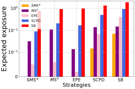
(a) Expected exposure

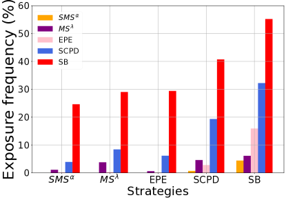
(b) Exposure frequency

Figure 9: Exposure analysis for a SAA-c game with five strategies

To analyse exposure, we plot in Figure 9a the expected exposure of each strategy $A$ against every strategy $B$ displayed on the x-axis. Similarly, we plot in Figure 9b the exposure frequency of each strategy $A$ against every strategy $B$ displayed on the x-axis. For instance, if $A=SMS^{\alpha}$ and $B=\text{SB}$, the expected exposure and exposure frequency of $SMS^{\alpha}$ against $SB$ are respectively $0.07$ and $4.4\%$. They both correspond respectively to the orange bar above index SB on the x-axis in Figure 9a and Figure 9b.

Firstly, in the situation where all bidders decide to play the same strategy, $SMS^{\alpha}$ has the remarkable property of never leading to exposure. This is not the case for the four other strategies. Secondly, $SMS^{\alpha}$ is the only strategy which never suffers from exposure against $MS^{\lambda}$ and EPE. Thirdly, even against SCDP and SB, $SMS^{\alpha}$ is rarely exposed. It has the lowest expected exposure and exposure frequency. For instance, $SMS^{\alpha}$ induces $9.3$, $4.5$, $34$ and $90$ times less expected exposure against SCPD than $MS^{\lambda}$, EPE, SCPD and SB respectively. Moreover, regarding exposure frequency, by playing $SMS^{\alpha}$ a bidder has $6.6$, $4$, $27.6$ and $58.1$ times less chance of ending up exposed against SCPD than $MS^{\lambda}$, EPE, SCPD and SB respectively.

Hence, not only does $SMS^{\alpha}$ achieve higher expected utility than state-of-the-art algorithms but it also takes less risks.

V-E Influence of $\alpha$

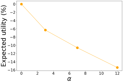
(a) Decrease in expected utility (%) when deviating from $SMS^{0}$ to $SMS^{\alpha}$ when all opponents play $SMS^{\alpha}$

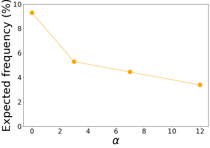
(b) Exposure frequency ($\%$) of $SMS^{\alpha}$ against SB versus $\alpha$

Figure 10: Impact of $\alpha$ on $SMS^{\alpha}$

Our strategy $SMS^{\alpha}$ is based on a risk-aversion hyperparameter $\alpha$. To show its impact on $SMS^{\alpha}$’s performance, we compare $SMS^{\alpha}$ for the following values of $\alpha$: $0$, $3$, $7$ and $12$.

Our first experiment is to study the impact of $\alpha$ on the expected utility of $SMS^{\alpha}$. We plot in Figure 10a the relative difference in expected utility between playing $SMS^{0}$ and $SMS^{\alpha}$ when all other bidders are playing $SMS^{\alpha}$. We observe that switching from $SMS^{0}$ to $SMS^{\alpha}$ leads to a loss in expected utility for any value $\alpha>0$. Moreover, this loss is an increasing function of $\alpha$. Similar results are obtained for the other three deviations in the empirical game where a bidder has the choice between either playing $SMS^{0}$ or $SMS^{\alpha}$. The fact that deviating to the risk-neutral strategy $SMS^{0}$ is always profitable and that the relative expected loss incurred by switching to $SMS^{\alpha}$ increases with $\alpha$ is far from surprising. Indeed, by increasing $\alpha$, a $SMS^{\alpha}$ bidder prefers bidding on sets of items which generates less utility but with less chance of leading to exposure.

To highlight the fact that increasing $\alpha$ leads to less exposure, we plot the exposure frequency of $SMS^{\alpha}$ against SB for different values of $\alpha$ in Figure 10b. We clearly see that the exposure frequency decreases when $\alpha$ grows. Indeed, an $SMS^{0}$ bidder has respectively $1.8$, $2.1$ and $2.7$ more chance of being exposed against SB than $SMS^{3}$, $SMS^{7}$ and $SMS^{12}$.

Moreover, increasing $\alpha$ also tackles the own price effect. For instance, the average price per item won when all bidders play $SMS^{\alpha}$ is respectively $3.11$, $2.48$, $2.21$ and $2$ for $\alpha$ equal to $0$, $3$, $7$ and $12$. This is a natural effect of risk-aversion where a bidder tends to avoid a rise in price. This mainly explains why we observe an increase in expected utility for the strategy profile where all bidders play $SMS^{\alpha}$ when $\alpha$ grows. For example, the expected utility when all bidders play $SMS^{12}$ is $1.36$ times greater than the expected utility when all bidders play $SMS^{0}$.

By increasing $\alpha$, $SMS^{\alpha}$ tackles more efficiently the exposure problem and own price effect. Thus, it minimises the risk of incurring a loss if bidders do not behave as expected. However, the main drawback is that it decreases one’s expected utility. The hyperparameter $\alpha$ thus allows the bidder to arbitrate between expected utility and risk-aversion.

VI Conclusions and Future Work

This paper introduces the first efficient bidding strategy that tackles simultaneously the exposure problem, the own price effect, budget constraints and the eligibility management problem in a simplified version of SAA (SAA-c). Our solution $SMS^{\alpha}$ largely outperforms state-of-the-art algorithms on instances of realistic size in generic settings.

It is a SM-MCTS whose expansion and rollout phase relies on a new method for the prediction of closing prices. This method is based on a specific sequence that has the advantage of converging in practice in all undertaken SAA-c instances, taking into account the auction’s mechanism and not relying solely on the outcomes of single specific strategy profile. We introduce scalarised rewards in $SMS^{\alpha}$ through a hyperparameter $\alpha$ giving the freedom to bidders to arbitrate between expected utility and risk-aversion. Increasing $\alpha$ reduces exposure and own price effect but decreases one’s expected utility.

In this paper, we have considered an auction where valuations and budgets are common knowledge. In order to apply $SMS^{\alpha}$ to incomplete information frameworks and, thus, deal with probability distributions, a simple approach is to compute their expectation and then consider the corresponding SAA-c game. We believe that, by updating beliefs each round and by better exploiting the probability distributions, further enhancements can be achieved. Future works should be guided in this direction.

References

- [1] ANACOM. Anacom commences procedure to amend the 5g auction regulation in order to prohibit use of smaller bidding increments. https://www.anacom.pt/render.jsp?contentId=1695741, 2021.
- [2] Kenneth Joseph Arrow, Frank Hahn, et al. General competitive analysis. 1971.
- [3] Lawrence M Ausubel, Peter Cramton, Marek Pycia, Marzena Rostek, and Marek Weretka. Demand reduction and inefficiency in multi-unit auctions. The Review of Economic Studies, 81(4):1366–1400, 2014.
- [4] Leon Barrett and Srini Narayanan. Learning all optimal policies with multiple criteria. In Proceedings of the 25th international conference on Machine learning, pages 41–47, 2008.
- [5] Sandro Brusco and Giuseppe Lopomo. Collusion via signalling in simultaneous ascending bid auctions with heterogeneous objects, with and without complementarities. The Review of Economic Studies, 69(2):407–436, 2002.
- [6] Sandro Brusco and Giuseppe Lopomo. Simultaneous ascending auctions with complementarities and known budget constraints. Economic Theory, 38(1):105–124, 2009.
- [7] Bundesnetzagentur. Spectrum for wireless access for the provision of telecommunications services. https://www.bundesnetzagentur.de/EN/Areas/Telecommunications/Companies/FrequencyManagement/ElectronicCommunicationsServices/ElectronicCommunicationServices_node.html, 2022.
- [8] Benjamin E Childs, James H Brodeur, and Levente Kocsis. Transpositions and move groups in monte carlo tree search. In 2008 IEEE Symposium On Computational Intelligence and Games, pages 389–395. IEEE, 2008.
- [9] Peter I Cowling, Edward J Powley, and Daniel Whitehouse. Information set monte carlo tree search. IEEE Transactions on Computational Intelligence and AI in Games, 4(2):120–143, 2012.
- [10] Peter Cramton et al. Spectrum auctions. Handbook of telecommunications economics, 1:605–639, 2002.
- [11] Peter Cramton et al. Simultaneous ascending auctions. Combinatorial auctions, pages 99–114, 2006.
- [12] European 5G Observatory. Italian 5g spectrum auction. https://5gobservatory.eu/italian-5g-spectrum-auction-2/, 2018.
- [13] Jacob K Goeree and Yuanchuan Lien. An equilibrium analysis of the simultaneous ascending auction. Journal of Economic Theory, 153:506–533, 2014.
- [14] Levente Kocsis and Csaba Szepesvári. Bandit based monte-carlo planning. In European conference on machine learning, pages 282–293. Springer, 2006.
- [15] Jongmin Lee, Geon hyeong Kim, Pascal Poupart, and Kee-Eung Kim. Monte-carlo tree search for constrained mdps. In IJCAI 2018, 2018.
- [16] Jongmin Lee, Geon-Hyeong Kim, Pascal Poupart, and Kee-Eung Kim. Monte-carlo tree search for constrained pomdps. Advances in Neural Information Processing Systems, 31, 2018.
- [17] Benny Lehmann, Daniel Lehmann, and Noam Nisan. Combinatorial auctions with decreasing marginal utilities. Games and Economic Behavior, 55(2):270–296, 2006.
- [18] Michael Maschler, Shmuel Zamir, and Eilon Solan. Game theory. Cambridge University Press, 2020.
- [19] Paul Milgrom. Putting auction theory to work: The simultaneous ascending auction. Journal of political economy, 108(2):245–272, 2000.
- [20] Paul Milgrom and Paul Robert Milgrom. Putting auction theory to work. Cambridge University Press, 2004.
- [21] Ofcom. Award of the 700 mhz and 3.6-3.8 ghz spectrum bands. Technical report, Ofcom, 2020. https://www.ofcom.org.uk/__data/assets/pdf_file/0020/192413/statement-award-700mhz-3.6-3.8ghz-spectrum.pdf.
- [22] Alexandre Pacaud, Marceau Coupechoux, and Aurelien Bechler. Monte carlo tree search bidding strategy for simultaneous ascending auctions. In 2022 20th International Symposium on Modeling and Optimization in Mobile, Ad hoc, and Wireless Networks (WiOpt), pages 322–329. IEEE, 2022.
- [23] Daniel M Reeves, Michael P Wellman, Jeffrey K MacKie-Mason, and Anna Osepayshvili. Exploring bidding strategies for market-based scheduling. Decision Support Systems, 39(1):67–85, 2005.
- [24] Maciej Świechowski, Konrad Godlewski, Bartosz Sawicki, and Jacek Mańdziuk. Monte carlo tree search: A review of recent modifications and applications. Artificial Intelligence Review, pages 1–66, 2022.
- [25] Balazs Szentes and Robert W Rosenthal. Beyond chopsticks: Symmetric equilibria in majority auction games. Games and Economic Behavior, 45(2):278–295, 2003.
- [26] Balázs Szentes and Robert W Rosenthal. Three-object two-bidder simultaneous auctions: chopsticks and tetrahedra. Games and Economic Behavior, 44(1):114–133, 2003.
- [27] Mandy JW Tak, Marc Lanctot, and Mark HM Winands. Monte carlo tree search variants for simultaneous move games. In 2014 IEEE Conference on Computational Intelligence and Games, pages 1–8. IEEE, 2014.
- [28] H Jaap Van Den Herik, Jos WHM Uiterwijk, and Jack Van Rijswijck. Games solved: Now and in the future. Artificial Intelligence, 134(1-2):277–311, 2002.
- [29] Robert J Weber. Making more from less: Strategic demand reduction in the fcc spectrum auctions. Journal of Economics & Management Strategy, 6(3):529–548, 1997.
- [30] Michael P Wellman, Anna Osepayshvilli, Jeffrey K MacKie-Mason, and Daniel Reeves. Bidding strategies for simultaneous ascending auctions. B.E. J. Theoret. Econom, 2008.
- [31] Charles Z Zheng. Jump bidding and overconcentration in decentralized simultaneous ascending auctions. Games and Economic Behavior, 76(2):648–664, 2012.
- [32] Albert L Zobrist. A new hashing method with application for game playing. ICGA Journal, 13(2):69–73, 1990.