Robust stabilization of $2\times 2$ first-order hyperbolic PDEs with uncertain input delay

Abstract

A backstepping-based compensator design is developed for a system of $2\times 2$ first-order linear hyperbolic partial differential equations (PDE) in the presence of an uncertain long input delay at boundary. We introduce a transport PDE to represent the delayed input, which leads to three coupled first-order hyperbolic PDEs. A novel backstepping transformation, composed of two Volterra transformations and an affine Volterra transformation, is introduced for the predictive control design. The resulting kernel equations from the affine Volterra transformation are two coupled first-order PDEs and each with two boundary conditions, which brings challenges to the well-posedness analysis. We solve the challenge by using the method of characteristics and the successive approximation. To analyze the sensitivity of the closed-loop system to uncertain input delay, we introduce a neutral system which captures the control effect resulted from the delay uncertainty. It is proved that the proposed control is robust to small delay variations. Numerical examples illustrate the performance of the proposed compensator.

1 Introduction

The compensator design for distributed parameter systems (DPS) with delay, which is molded by PDEs, has been given much concern and study [1, 2, 3]. Delays widely exist in industrial process fields and common phenomena, yet even minor delays may destabilize the system or cause accidents. Hence, the compensation control of delay is an active topic. The main methods of spectrum decomposition [1, 4], Lyapunov function technique [5], fuzzy control [6], Hilbert space theory [7], and backstepping approach [8] are utilized to stabilize such systems with delay.

As well known, unbounded control operators based on the backstepping method have been considered for both hyperbolic equations [9], heat equations [10, 11], wave equations, and some high-dimensional PDE systems[12], where delays are compensated. Not only delay compensation design, but also a series of problems in DPS can be solved by backstepping method: motion planning [13], adaptive controller design [14, 15] and output regulation problem [16, 17], etc. Among them is a class of PDE systems, $2\times 2$ first-order hyperbolic PDEs, which can be used to describe various industrial processes and phenomena, such as traffic flow [18], hydraulics and river dynamics [19, 20], pipeline networks [21] and so on. [22] stabilizes $2\times 2$ linear system by backstepping method, which is the foundation of subsequent works, and further, extending to quasi-linear system in [23]. The more general stabilization problem of a class of $m+1$ and $m+n$ hyperbolic PDEs system are addressed in [24, 25]. The disturbance rejection and observer design for hyperbolic systems have been focused on in [26, 27] and [28], respectively. An event-triggered boundary control is proposed in [29], where the sensor delay is compensated.

The delay-compensated control design is more challenging for uncertain coupled hyperbolic systems. One way for robustly stabilizing a $2\times 2$ linear hyperbolic system against possible actuator delay by preserving a small amount of the proximal reflection is presented in [30]. Similarly, a $m+n$ hyperbolic PDEs system is considered in [31]. An underactuated cascade network of $n$ systems of two heterodirectional hyperbolic PDEs is considered in [32], which utilizes a two-step integral transformation to move the in-domain coupling terms to the boundary. In addition, the method of combining with a low-pass filter and a controller based on prediction is proposed in [33], for solving the robust stabilization problem of an underactuated network of two subsystems of heterodirectional $n+m$ hyperbolic system. The method for recursively handling multiple cascaded subsystems is also applied to stabilize systems that concatenate multiple hyperbolic PDEs and an ODE [34, 35].

Another approach to address uncertain delays is to design adaptive control laws using existing stability results. For instance, the $2\times 2$ hyperbolic system with input delay and sensor delay is equivalent to a delay-free system in [36] through a series of transformations; then the existing adaptive control law can be employed.

This paper provides a distinctive way of stabilization of the $2\times 2$ hyperbolic system subject to an uncertain input delay. First, the exact system is taken into account. A transport PDE is introduced to represent the delayed input, which results in three coupled cascade first-order hyperbolic PDEs. Unlike the existing references which apply multi-step transformation in the control design, such as [30], we propose a more direct way to solve the delay-compensation problem by introducing a single-step backstepping transformation composed of two Volterra transformations and an affine Volterra transformation. The affine Volterra transformation includes both the integration of the states and that of the delayed actuator state governed by the transport PDE. The resulting kernel equations of the affine Volterra transformation are coupled both in the domain equations and in the boundary conditions. Besides, there are two boundary conditions for each kernel, which leads to each kernel being defined in multiple subregions. Due to these two facts, it is challenging to prove the well-posedness of the kernel equations. The challenge is solved by combining the method of characteristics and the successive approximation.

In line with the transformation, the control law consists of the feedback of the states and the feedback of historical control input. The finite-time stability of closed-loop systems with delay-compensated control is proved. Furthermore, we analyze the robustness of the delay-compensated control for the uncertain input delay through the equivalent neutral system. Finally, compared with the controller without delay compensation, the control effect of the proposed compensator is illustrated.

The contribution of this paper is summarized as:

1. Compared to the results in [30, 34, 35] about robust stabilization of hyperbolic system with small actuator delay, we propose an arbitrary long delay-compensated control design method and analyze the robustness of the controller with small delay variation.

2. We develop a novel single-step backstepping transformation that is more straightforward than the multi-step transformation used in [32, 36] because it avoids multi-step inverse transformation to reach the final form of the control law. The resulting kernel equations appear more complicated form than that of [22] due to each kernel equation having two boundary conditions. We combine the method of characteristics and the successive approximation to prove that the kernel equations, where each kernel function is defined in multiple subregions, are well-posed.

This paper is organized as follows. Section 2 gives the problem formulation. The backstepping-based compensation controller is established in Section 3. In Section 4, well-posedness of the kernels is discussed, which is one of the main technical contribution of this paper. The finite-time stability of the closed-loop system that is subjected to exact input delay is summarized in section 5. In Section 6, we prove that the proposed control law still stabilizes the hyperbolic system if there is small variation in the input delay, which also is one of the technical contributions of this paper. The simulation results are presented in Section 7 to validate the effectiveness of the proposed compensator. The paper ends with concluding remarks and a discussion of the future work in Section 8.

2 Problem formulation

Consider the following $2\times 2$ first-order linear hyperbolic PDEs with input delay $\tau\in R^{+}$,

$$\partial_{t}u_{1}(x,t)= ~{}-\varepsilon_{1}(x)\partial_{x}u_{1}(x,t)+c_{1}(x)u_{2}(x,t),$$ (1a)

$$\partial_{t}u_{2}(x,t)= ~{}\varepsilon_{2}(x)\partial_{x}u_{2}(x,t)+c_{2}(x)u_{1}(x,t),$$ (1b)

$$u_{1}(0,t)= ~{}qu_{2}(0,t),$$ (1c)

$$u_{2}(1,t)= ~{}U(t-\tau),$$ (1d)

$$U(t-h)= ~{}0,\quad h\in[0,\tau],$$ (1e)

for $(x,t)\in[0,1]\times\mathbb{R}^{+}$, with the initial conditions,

$$u_{1}(x,0)=u_{10}(x)\in\mathbb{C}([0,1]),$$ (2a)

$$u_{2}(x,0)=u_{20}(x)\in\mathbb{C}([0,1]),$$ (2b)

and where the coefficients $q\in\mathbb{R}^{+}$, $\varepsilon_{1}(x)$, $\varepsilon_{2}(x),c_{1}(x)$, $c_{2}(x)\in\mathbb{C}([0,1])$ and transport velocities $\varepsilon_{1}(x),\,\varepsilon_{2}(x)\textgreater 0$. Here, $\partial_{x}u(x,t)={\partial u}/{\partial x}$ and $\partial_{t}u(x,t)={\partial u}/{\partial t}$ are represented in a compact form of partial derivative.

The control objective of this paper is to design a compensated controller to ensure that the closed-loop system is exponentially stable, in particular, reaching the zero-equilibrium state in finite time. Based on the relation between the first-order hyperbolic PDE and delay equations [37], a transport PDE is introduced to express the input delay, so the system (1) is rewritten as follows:

$$\partial_{t}u_{1}(x,t) =-\varepsilon_{1}(x)\partial_{x}u_{1}(x,t)+c_{1}(x)u_{2}(x,t),$$ (3a)

$$\partial_{t}u_{2}(x,t) =\varepsilon_{2}(x)\partial_{x}u_{2}(x,t)+c_{2}(x)u_{1}(x,t),$$ (3b)

$$u_{1}(0,t) =qu_{2}(0,t),$$ (3c)

$$u_{2}(1,t) =v(0,t),$$ (3d)

$$\tau\partial_{t}v(x,t) =\partial_{x}v(x,t),$$ (3e)

$$v(1,t) =U(t),$$ (3f)

with the initial condition $v(x,0)=v_{0}(x)\in\mathbb{C}([0,1])$.

3 Controller design

3.1 Backstepping control design

Following the backstepping approach [38], we introduce two Volterra transformations and an affine Volterra transformation integral transformation as follows:

$$w_{1}(x,t)= ~{}u_{1}(x,t)-\int_{0}^{x}K^{11}(x,y)u_{1}(y,t)\,\mathrm{d}y$$

$$~{}-\int_{0}^{x}K^{12}(x,y)u_{2}(y,t)\,\mathrm{d}y,$$ (4a)

$$w_{2}(x,t)= ~{}u_{2}(x,t)-\int_{0}^{x}\!K^{21}(x,y)u_{1}(y,t)\,\mathrm{d}y$$

$$~{}-\int_{0}^{x}K^{22}(x,y)u_{2}(y,t)\,\mathrm{d}y,$$ (4b)

$$z(x,t)= ~{}v(x,t)-\int_{0}^{x}p(x-y)v(y,t)\,\mathrm{d}y$$ (4c)

$$-\int_{0}^{1} \alpha_{1}(x,y)u_{1}(y,t)\,\mathrm{d}y-\int_{0}^{1}\alpha_{2}(x,y)u_{2}(y,t)\,\mathrm{d}y,$$

where the kernel functions $K^{ij}(x,y)$, $i,j=1,2$, are to be defined on the triangular domain $\mathcal{T}_{1}=\left\{(x,y)\in\mathbb{R}^{2}:0\leq y\leq x\leq 1\right\}$, the kernel functions $\alpha_{1}(x,y)$, $\alpha_{2}(x,y)$ are to be defined on the rectangle domain $\mathcal{T}_{2}=\left\{(x,y)\in\mathbb{R}^{2}:0\leq x,\,y\leq 1\right\}$, and the kernel function $p(x)\in L^{2}([0,1])$.

Then, we find sufficient conditions on these functions, such that transformations (4) map system (3) to the following system

$$\partial_{t}w_{1}(x,t) =-\varepsilon_{1}(x)\partial_{x}w_{1}(x,t),$$ (5a)

$$\partial_{t}w_{2}(x,t) =\varepsilon_{2}(x)\partial_{x}w_{2}(x,t),$$ (5b)

$$w_{1}(0,t) =qw_{2}(0,t),$$ (5c)

$$w_{2}(1,t) =z(0,t),$$ (5d)

$$\tau\partial_{t}z(x,t) =\partial_{x}z(x,t),$$ (5e)

$$z(1,t) =0.$$ (5f)

Combined with system (3), differentiate the mapping (4) with respect to space and time respectively, and then substitute it into the target system (5), one obtains that the kernels $K^{ij}$, $i,j=1,2$, satisfy a set of hyperbolic PDEs given in [23], and the kernels $\alpha_{1}$, $\alpha_{2}$ satisfy:

$$\frac{1}{\tau}\partial_{x}\alpha_{1}-\varepsilon_{1}(y) \partial_{y}\alpha_{1}=\varepsilon_{1}^{\prime}(y)\alpha_{1}(x,y)+c_{2}(y)\alpha_{2},$$ (6a)

$$\frac{1}{\tau}\partial_{x}\alpha_{2}+\varepsilon_{2}(y) \partial_{y}\alpha_{2}=-\varepsilon_{2}^{\prime}(y)\alpha_{2}+c_{1}(y)\alpha_{1},$$ (6b)

with the boundary conditions

$$\alpha_{1}(x,1)= ~{}0,$$ (7a)

$$\varepsilon_{2}(0)\alpha_{2}(x,0)= ~{}q\varepsilon_{1}(0)\alpha_{1}(x,0),$$ (7b)

$$\alpha_{1}(0,y)= ~{}K^{21}(1,y),$$ (7c)

$$\alpha_{2}(0,y)= ~{}K^{22}(1,y).$$ (7d)

After solving $\alpha_{2}(x,y)$, the kernel $p(x)$ has the following form

$$p(x)=\tau\varepsilon_{2}(1)\alpha_{2}(x,1).$$ (8)

After obtaining all the kernels, we discuss the form of compensator. Substituting boundary conditions (3f) and (5f) into transformation (4c), the controller is obtained in the following form:

$$U(t)= ~{}\int_{0}^{1}p(1-y)v(y,t)\,\mathrm{d}y+\int_{0}^{1}\alpha_{1}(1,y)u_{1}(y,t)\,\mathrm{d}y$$

$$~{}+\int_{0}^{1}\alpha_{2}(1,y)u_{2}(y,t)\,\mathrm{d}y.$$ (9)

Then, using the method of characteristics and variable substitution for (3.1), the controller with delay compensation can be written in the following form:

$$U(t)= \int_{0}^{1}\alpha_{1}(1,y)u_{1}(y,t)\,\mathrm{d}y+\int_{0}^{1}\alpha_{2}(1,y)u_{2}(y,t)\,\mathrm{d}y$$

$$\int_{t-\tau}^{t}p\left(\frac{t-y}{\tau}\right)U(y)\,\mathrm{d}y.$$ (10)

4 Well-posedness of the kernel functions

The well-posedness of the kernel functions $K^{ij}$, $i,j=1,2$ have given in [23]. Here we discuss the well-posedness of $\alpha_{1}$ and $\alpha_{2}$, because they have two boundary conditions which make them different from kernels $K^{ij}$ or $L^{ij}$ with only one boundary condition in a triangle domain. Define a general form of equations $\alpha_{1}$-$\alpha_{2}$ as follows:

$$\frac{\partial_{x}F_{1}}{\tau}-\varepsilon_{1}(y)\partial_{y}F =g_{1}(x,y)+\sum_{k=1}^{2}C_{1k}(x,y)F_{k},$$ (11a)

$$\frac{\partial_{x}F_{2}}{\tau}+\varepsilon_{2}(y)\partial_{y}F_{2} =\!g_{2}(x,y)+\sum_{k=1}^{2}C_{2k}(x,y)F_{k},$$ (11b)

evolving in the domain $\mathcal{T}_{2}$, with boundary conditions

$$F_{1}(x,1) =0,$$ (12a)

$$F_{1}(0,y) =h_{1}(y),$$ (12b)

$$F_{2}(x,0) =q_{1}(x)F_{1}(x,0),$$ (12c)

$$F_{2}(0,y) =h_{2}(y).$$ (12d)

The well-posedness of equations (11) and (12) is presented in the following theorem.

Theorem 1.

Consider the hyperbolic system (11) with the boundary condition (12). Under the assumptions $q_{1}(x),h_{i}(x)\in\mathbb{C}([0,1])$, $\varepsilon_{i}(x)\in\mathbb{C}([0,1])$ with $\varepsilon_{i}(x)\textgreater 0$ and $C_{ij}(x,y)\in\mathcal{T}_{2}$, $i,j=1,2$, there exists a unique solution $F_{k}\in\mathbb{C}(\mathcal{T}_{2})$, $k=1,2$.

The proof of this theorem is divided into two steps. First, we transform the coupled equations into integral equations using the method of characteristics, which is presented in Section 4.1, and then solve it by successive approximation method, which is presented in Section 4.2.

4.1 Integral equation

First, define

$$\phi_{1}(x)=\int_{0}^{x}\frac{1}{\varepsilon_{1}(\zeta)}\,\mathrm{d}\zeta,\quad\phi_{2}(x)=\int_{0}^{x}\frac{1}{\varepsilon_{2}(\zeta)}\,\mathrm{d}\zeta.$$ (13)

Note that since the propagation velocities $\varepsilon_{1}(x)$ and $\varepsilon_{2}(x)$ are both positive, all $\phi_{i}(x)$, $i=1,2$ functions are monotonically increasing and invertible. Also, it holds that $\phi_{i},\phi_{i}^{-1}\in\mathbb{C}([0,1])$.

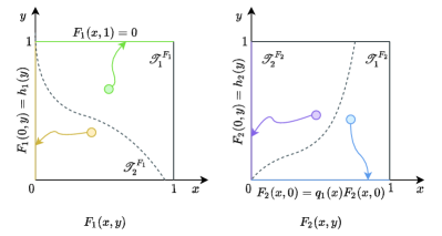
Figure 1: Diagram of characteristic curves. Different color curves represent characteristic curves affected by corresponding boundary conditions.

The characteristic curves of $F_{1}(x,y)$ and $F_{2}(x,y)$ are depicted in Fig. 1. According to the distribution of the characteristic curves, $F_{1}(x,y)$ is defined in two regions $\mathcal{T}^{F_{1}}_{1}$ and $\mathcal{T}^{F_{1}}_{2}$, and $F_{2}(x,y)$ in $\mathcal{T}^{F_{2}}_{1}$ and $\mathcal{T}^{F_{2}}_{2}$, which are shown in Fig. 1. It is means that, for instance, when solving the characteristic (14a)–(14b) backward from a given point in $\mathcal{T}^{F_{1}}_{1}$, one “hits” the boundary depicted in green on Fig. 1.

(1) Characteristics of the $F_{1}(x,y)$: For $(x,y)\in\mathcal{T}_{2}$, define the characteristic curves as follows, along which the system (11a) becomes a family of ordinary differential equations,

$$x_{11}(x,y,s)= ~{}x+\frac{s-\phi_{1}(1)+\phi_{1}(y)}{\tau},s\in[0,s_{11}]$$ (14a)

$$y_{11}(x,y,s)= ~{}\phi_{1}^{-1}(\phi_{1}(1)-s),\qquad\quad\,s\in[0,s_{11}]$$ (14b)

$$x_{12}(x,y,s)= ~{}\frac{s}{\tau},\qquad\qquad\qquad\qquad\,\,\,\,\,s\in[0,s_{12}]$$ (14c)

$$y_{12}(x,y,s)= ~{}\phi_{1}^{-1}(\tau x+\phi_{1}(y)-s),\,\,\,\,\,s\in[0,s_{12}]$$ (14d)

where the argument $s\in[0,s_{1j}]$, $j=1,\,2$, with $s_{1j}$ defined as

$$s_{11}(x,y)= ~{}\phi_{1}(1)-\phi_{1}(y),$$ (15a)

$$s_{12}(x,y)= ~{}\tau x.$$ (15b)

(2) Characteristics of the $F_{2}(x,y)$: For $(x,y)\in\mathcal{T}_{2}$, define the characteristic curves as follows, along which the system (11b) becomes a family of ordinary differential equations,

$$x_{21}(x,y,s)= ~{}x+\frac{s}{\tau}-\frac{\phi_{2}(y)}{\tau}, s\in[0,s_{21}]$$ (16a)

$$y_{21}(x,y,s)= ~{}\phi_{2}^{-1}(s), s\in[0,s_{21}]$$ (16b)

$$x_{22}(x,y,s)= ~{}\frac{s}{\tau}, s\in[0,s_{22}]$$ (16c)

$$y_{22}(x,y,s)= ~{}\phi_{2}^{-1}(\tau x+\phi_{2}(y)-s), s\in[0,s_{22}]$$ (16d)

where the argument $s\in[0,s_{2j}]$, $j=1,\,2$, with $s_{2j}$ defined as

$$s_{21}(x,y)= ~{}\phi_{2}(y),$$ (17a)

$$s_{22}(x,y)= ~{}\tau x.$$ (17b)

Integrating (11a) along the characteristic curves defined by (14a)–(14b) and (14c)–(14d), respectively, and considering boundary conditions (12a) and (12b), respectively, the solution of $F_{1}(x,y)$ is yielded,
a) for each $(x,y)\in\mathcal{T}^{F_{1}}_{1}$,

$$F_{1}(x,y) =G_{11}(x,y)+I_{11}[F](x,y),$$ (18)

b) for each $(x,y)\in\mathcal{T}^{F_{1}}_{2}$,

$$F_{1}(x,y) =H_{1}(x,y)+G_{12}(x,y)+I_{12}[F](x,y),$$ (19)

where $F$ is denoted $F=\begin{bmatrix}F_{1}&F_{2}\end{bmatrix}^{\mathrm{T}}$, and the functions $H_{1}$, $G_{1j}$ and $I_{1j}$, for $j=1,\,2$, will be defined later.

Similarly, integrating (11b) along the characteristic curves defined by (16a)–(16b) and (16c)–(16d), respectively, and considering boundary conditions (12c) and (12d), respectively, the solution of $F_{2}(x,y)$ is yielded,
a) for each $(x,y)\in\mathcal{T}^{F_{2}}_{1}$,

$$F_{2}=Q_{1}(x)F_{1}(x,0)+G_{21}(x,y)+I_{21}[F](x,y),$$ (20)

b) for each $(x,y)\in\mathcal{T}^{F_{2}}_{2}$,

$$F_{2} =H_{2}(x,y)+G_{22}(x,y)+I_{22}[F](x,y),$$ (21)

where the functions $H_{i}$, $G_{ij}$ and $I_{ij}$, $i,\,j=1,\,2$ are defined as

$$H_{i}(x,y)=h_{i}\big{(}y_{i2}(x,y,0)\big{)},$$ (22a)

$$G_{ij}(x,y)=\!\int_{0}^{s_{ij}(x,y)}\!\!\!\!\!\!g_{i}\big{(}x_{ij}(x,y,s),y_{ij}(x,y,s)\big{)}\,\mathrm{d}s,$$ (22b)

$$I_{ij}[F](x,y)=\sum_{k=1}^{2}\int_{0}^{s_{ij}(x,y)}C_{ik}\big{(}x_{ij}(x,y,s),y_{ij}(x,y,s)\big{)}\cdot$$

$$\quad\quad\quad\quad\quad F_{k}\big{(}x_{ij}(x,y,s),y_{ij}(x,y,s)\big{)}\,\mathrm{d}s.$$ (22c)

Then, according to (18) and (19), substituting $F_{1}(x,0)$ to (20), the integral form of $F_{2}$ is rewritten as:
a) for each $(x,y)\in\mathcal{T}^{F_{1}}_{1}\cap\mathcal{T}^{F_{2}}_{1}$,

$$F_{2}(x,y)= \psi_{1}(x,y)+Q_{11}[F](x,y)+G_{21}(x,y)$$

$$~{}+I_{21}[F](x,y),$$ (23)

b) for each $(x,y)\in\mathcal{T}^{F_{1}}_{2}\cap\mathcal{T}^{F_{2}}_{1}$,

$$F_{2}(x,y)= ~{}\psi_{2}(x,y)+Q_{12}[F](x,y)+G_{21}(x,y)$$

$$~{}+I_{21}[F](x,y),$$ (24)

c) for each $(x,y)\in\mathcal{T}^{F_{2}}_{2}$,

$$F_{2}(x,y)=H_{2}(x,y)+G_{22}(x,y)+I_{22}[F](x,y),$$ (25)

where

$$\psi_{1}= ~{}q_{1}(x_{21}(x,y,0))G_{11}(x_{21}(x,y,0),0),$$ (26a)

$$\psi_{2}= ~{}q_{1}(x_{22}(x,y,0))H_{1}(x_{22}(x,y,0),0)$$

$$~{}+q_{1}(x_{22}(x,y,0))G_{12}(x_{22}(x,y,0),0),$$ (26b)

$$Q_{11}[F]= ~{}q_{1}(x_{21}(x,y,0))I_{11}[F](x_{21}(x,y,0),0),$$ (26c)

$$Q_{12}[F]= ~{}q_{1}(x_{22}(x,y,0))I_{12}[F](x_{22}(x,y,0),0).$$ (26d)

4.2 Convergence of the successive approximation series

Before proceeding, we first give the following lemmas.

Lemma 1.

If $(x,y)\in\mathcal{T}_{2}$ and $s\in[0,s_{ij}]$, it holds that $(x_{ij}(x,y,s),y_{ij}(x,y,s))\in\mathcal{T}_{2}$ for $i,\,j=1,\,2$. Also, under the assumptions of Theorem 1, $x_{ij}$, $y_{ij}$, and $s_{ij}$ are continuous in their domains of definition since they are defined as compositions of continuous functions. Moreover, the following inequalities are verified:

$$x_{11}(x,y,s) \leq x,\quad y_{11}(x,y,s)\geq y,$$ (27a)

$$x_{12}(x,y,s) \leq x,\quad y_{12}(x,y,s)\geq y,$$ (27b)

$$x_{21}(x,y,s) \leq x,\quad y_{21}(x,y,s)\leq y,$$ (27c)

$$x_{22}(x,y,s) \leq x,\quad y_{22}(x,y,s)\geq y.$$ (27d)

The proof of this lemma is obvious, so it is omitted. This lemma is used in the proof of Lemma 2.

Lemma 2.

For $n\in\mathbb{R}^{+}$, $i,\,j=1,2$, the following inequalities hold:

$$\int_{0}^{s_{ij}(x,y)}x_{ij}^{n}(x,y,s)\,\mathrm{d}s\leq M_{\varepsilon}\frac{x^{n+1}}{n+1},$$ (28)

Similar to Lemma A.4 of [23], we can obtain this lemma by utilizing variable substitution and Lemma 1.

In this section, the successive approximation method is employed to prove that there is a solution of the system (11) with the boundary condition (12). We start by defining the recursive equations for (18)–(19) and (23)–(25) as follows, with $n=0,1,2,\cdots,+\infty$,

$$F_{1}^{n+1}(x,y)=\begin{cases}I_{11}[F^{n}](x,y),&\mathcal{T}^{F_{1}}_{1},\\ I_{12}[F^{n}](x,y),&\mathcal{T}^{F_{1}}_{2},\end{cases}$$ (29a)

$$F_{2}^{n+1}(x,y)=$$ (29b)

$$\begin{cases}Q_{11}(x)[F^{n}](x,y)+I_{21}[F^{n}](x,y),&\mathcal{T}^{F_{1}}_{1}\cap\mathcal{T}^{F_{2}}_{1},\\ Q_{12}(x)[F^{n}](x,y)+I_{21}[F^{n}](x,y),&\mathcal{T}^{F_{1}}_{2}\cap\mathcal{T}^{F_{2}}_{1},\\ I_{22}[F^{n}](x,y),&\mathcal{T}^{F_{2}}_{2},\end{cases}$$

with an initial function

$$F_{1}^{0}(x,y) =\begin{cases}G_{11}(x,y),&\mathcal{T}^{F_{1}}_{1},\\ H_{1}(x,y)+G_{12}(x,y),&\mathcal{T}^{F_{1}}_{2},\end{cases}$$ (30a)

$$F_{2}^{0}(x,y) =\begin{cases}\psi_{1}(x,y)+G_{21}(x,y),&\mathcal{T}^{F_{1}}_{1}\cap\mathcal{T}^{F_{2}}_{1},\\ \psi_{2}(x,y)+G_{21}(x,y),&\mathcal{T}^{F_{1}}_{2}\cap\mathcal{T}^{F_{2}}_{1},\\ H_{2}(x,y)+G_{22}(x,y),&\mathcal{T}^{F_{2}}_{2}.\end{cases}$$ (30b)

It is easy to see that, if $\sum_{n=0}^{+\infty}F^{n}(x,y)$ converges, then $F(x,y)$ can be alternatively written as $F(x,y)=\sum_{n=0}^{+\infty}F^{n}(x,y)$, where $F^{n}$ is denoted as $F^{n}=\begin{bmatrix}F_{1}^{n}&F_{2}^{n}\end{bmatrix}^{\mathrm{T}}$.

Next, we discuss the convergence of series by successive approximation. Define

$$\bar{C}_{ij}= ~{}\max_{(x,y)\in\mathcal{T}_{ij}}\left\{|C_{ij}(x,y)|,\,|\partial_{x}C_{ij}(x,y)|\right\},$$ (31a)

$$\bar{q}= ~{}\max_{(x)\in[0,1]}\left\{|q_{1}(x)|,\,|\partial_{x}q_{1}(x)|\right\},$$ (31b)

$$M_{0}= ~{}\max\Bigg{\{}|F_{1}^{0}|,\,|F_{2}^{0}|,\,2\sum_{k=1}^{2}\bar{C}_{ik}|F_{k}^{0}|,$$ (31c)

$$~{}\qquad\qquad\left(2\bar{q}\sum_{k=1}^{2}\bar{C}_{1k}+\sum_{k=1}^{2}\bar{C}_{2k}\right)|F_{k}^{0}|\Bigg{\}},$$ (31d)

$$M_{\varepsilon}= ~{}\max\left\{\tau,\,\frac{1}{\varepsilon_{1}(x)},\,\frac{1}{\varepsilon_{2}(x)}\right\},$$ (31e)

$$\bar{C}= ~{}\max\left\{3\bar{q}\sum_{k=1}^{2}\!\bar{C}_{1k}\!+\!2\sum_{k=1}^{2}\!\bar{C}_{2k},\,3\sum_{k=1}^{2}\!\bar{C}_{ik},\right\}\!,$$ (31f)

with $i,j=1,2$. Assume that for $n\in N^{+}$,

$$\left|F^{n}(x,y)\right|\leq M_{0}\frac{(\bar{C}M_{\varepsilon}x)^{n}}{n!},$$ (32)

holds, using induction method, we discuss whether $F^{n+1}(x,y)$ satisfies the above inequalities in different domain. From (29) and (32), using Lemma 2, we have:
(1) for $F_{1}^{n+1}$ on $\mathcal{T}_{1}^{F_{1}}$,

$$~{}\left|F_{1}^{n+1}(x,y)\right|=\left|I_{11}[F^{n}](x,y)\right|$$

$$\leq ~{}\sum_{k=1}^{2}\int_{0}^{s_{11}(x,y)}\Big{|}C_{1k}\big{(}x_{11}(x,y,s),y_{11}(x,y,s)\big{)}\cdot$$

$$~{}\qquad\qquad F_{k}^{n}\big{(}x_{11}(x,y,s),y_{11}(x,y,s)\big{)}\Big{|}\,\mathrm{d}s$$

$$\leq ~{}M_{0}\frac{(\bar{C}M_{\varepsilon})^{n}}{n!}\sum_{k=1}^{2}\bar{C}_{1k}\int_{0}^{s_{11}(x,y)}x_{11}^{n}(x,y,s)\,\mathrm{d}s$$

$$\leq ~{}M_{0}\frac{(\bar{C}M_{\varepsilon}x)^{n+1}}{(n+1)!},$$ (33)

(2) for $F_{1}^{n+1}$ on $\mathcal{T}_{2}^{F_{1}}$,

$$~{}\left|F_{1}^{n+1}(x,y)\right|=\left|I_{12}[F^{n}](x,y)\right|$$

$$\leq ~{}\sum_{k=1}^{2}\int_{0}^{s_{12}(x,y)}\Big{|}C_{1k}\big{(}x_{12}(x,y,s),y_{12}(x,y,s)\big{)}\cdot$$

$$~{}\qquad\qquad F_{k}^{n}\big{(}x_{12}(x,y,s),y_{12}(x,y,s)\big{)}\Big{|}\,\mathrm{d}s$$

$$\leq ~{}M_{0}\frac{(\bar{C}M_{\varepsilon})^{n}}{n!}\sum_{k=1}^{2}\bar{C}_{1k}\int_{0}^{s_{12}(x,y)}x_{12}^{n}(x,y,s)\,\mathrm{d}s$$

$$\leq ~{}M_{0}\frac{(\bar{C}M_{\varepsilon}x)^{n+1}}{(n+1)!},$$ (34)

(3) for $F_{2}^{n+1}$ on $\mathcal{T}_{1}^{F_{2}}\cap\mathcal{T}_{1}^{F_{1}}$,

$$~{}\left|F_{2}^{n+1}(x,y)\right|=\left|Q_{11}(x)[F^{n}](x,y)+I_{21}[F^{n}](x,y)\right|$$

$$\leq ~{}\left|q_{1}(x_{21}(x,y,0))I_{11}[F^{n}](x_{21}(x,y,0),0)\right|$$

$$+\sum_{k=1}^{2}\int_{0}^{s_{21}(x,y)}\Big{|}C_{2k}\big{(}x_{21}(x,y,s),y_{21}(x,y,s)\big{)}\cdot$$

$$~{}\qquad\qquad F_{k}^{n}\big{(}x_{21}(x,y,s),y_{21}(x,y,s)\big{)}\Big{|}\,\mathrm{d}s$$

$$\leq ~{}\bar{q}\sum_{k=1}^{2}\int_{0}^{s_{21}(x_{21}(x,y,0),0)}\Big{|}C_{1k}\big{(}x_{21}(x,y,0),0\big{)}\cdot$$

$$~{}\qquad\qquad\qquad\qquad F_{k}\big{(}x_{21}(x,y,0),0\big{)}\Big{|}\,\mathrm{d}s$$

$$~{}+\sum_{k=1}^{2}\int_{0}^{s_{21}(x,y)}\Big{|}C_{2k}\big{(}x_{21}(x,y,s),y_{21}(x,y,s)\big{)}\cdot$$

$$~{}\qquad\qquad\qquad F_{k}^{n}\big{(}x_{21}(x,y,s),y_{21}(x,y,s)\big{)}\Big{|}\,\mathrm{d}s$$

$$\leq ~{}\bar{q}M_{0}\frac{\bar{C}^{n}M_{\varepsilon}^{n+1}}{n!}\sum_{k=1}^{2}\bar{C}_{1k}x_{21}^{n+1}(x,y,0)$$

$$~{}+M_{0}\frac{(\bar{C}^{n}M_{\varepsilon}^{n+1})}{n!}\sum_{k=1}^{2}\bar{C}_{2k}x^{n+1}$$

$$\leq ~{}\left(\bar{q}\sum_{k=1}^{2}\bar{C}_{1k}+\sum_{k=1}^{2}\bar{C}_{2k}\right)M_{0}\frac{\bar{C}^{n}M_{\varepsilon}^{n+1}x^{n+1}}{(n+1)!}$$

$$\leq ~{}M_{0}\frac{(\bar{C}M_{\varepsilon}x)^{n+1}}{(n+1)!},$$ (35)

(4) for $F_{2}^{n+1}$ on $\mathcal{T}_{1}^{F_{2}}\cap\mathcal{T}_{2}^{F_{1}}$,

$$~{}\left|F_{2}^{n+1}(x,y)\right|=\left|Q_{12}(x)[F^{n}](x,y)+I_{21}[F^{n}](x,y)\right|$$

$$\leq ~{}\left|q_{1}(x_{22}(x,y,0))I_{12}[F](x_{22}(x,y,0),0)\right|$$

$$~{}+\sum_{k=1}^{2}\int_{0}^{s_{21}(x,y)}\Big{|}C_{2k}\big{(}x_{21}(x,y,s),y_{21}(x,y,s)\big{)}\cdot$$

$$~{}\qquad\qquad\qquad F_{k}^{n}\big{(}x_{21}(x,y,s),y_{21}(x,y,s)\big{)}\Big{|}\,\mathrm{d}s$$

$$\leq ~{}M_{0}\frac{(\bar{C}M_{\varepsilon}x)^{n+1}}{(n+1)!},$$ (36)

(5) for $F_{2}^{n+1}$ on $\mathcal{T}_{2}^{F_{2}}$,

$$~{}\left|F_{2}^{n+1}(x,y)\right|=\left|I_{22}[F^{n}](x,y)\right|$$

$$~{}\leq\sum_{k=1}^{2}\int_{0}^{s_{22}(x,y)}\Big{|}C_{2k}\big{(}x_{22}(x,y,s),y_{22}(x,y,s)\big{)}\cdot$$

$$~{}\qquad\qquad\qquad F_{k}^{n}\big{(}x_{22}(x,y,s),y_{22}(x,y,s)\big{)}\Big{|}\,\mathrm{d}s$$

$$\leq ~{}M_{0}\frac{(\bar{C}M_{\varepsilon})^{n}}{n!}\sum_{k=1}^{2}\bar{C}_{2k}\int_{0}^{s_{22}(x,y)}x_{22}^{n}(x,y,s)\,\mathrm{d}s$$

$$\leq ~{}M_{0}\frac{(\bar{C}M_{\varepsilon}x)^{n+1}}{(n+1)!}.$$ (37)

Thus, by induction we have proved that (32) holds. Once the assumed value (32) is proved, it conclude that the series is bounded and converges uniformly,

$$\left|\sum_{n=0}^{+\infty}F^{n}(x,y)\right|\leq\sum_{n=0}^{+\infty}M_{0}\frac{(\bar{C}M_{\varepsilon}x)^{n}}{n!}=M_{0}\rm{e}^{\bar{C}M_{\varepsilon}x}.$$ (38)

Thus, it is proved that the system (11) with the boundary condition (12) has a bounded solution $F(x,y)$.

Next, we discuss the uniqueness of solution, assuming that two different solutions of (11)–(12) are denoted by $F(x,y)$ and $F^{\prime}(x,y)$. Define $\tilde{F}(x,y)=F(x,y)-F^{\prime}(x,y)$. Due to the linearity of (11)–(12), $\tilde{F}(x,y)$ also verifies (11)–(12), with $q_{1}(x)=0$, $g_{i}(x,y)=0$ and $h_{i}(y)=0$, $i=1,\,2$. It is easy to get that $M_{0}=0$ for $\tilde{F}(x,y)$, so we get $\tilde{F}(x,y)=0$, which means $F(x,y)=F^{\prime}(x,y)$. Thus, Theorem 1 is proved.

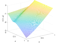
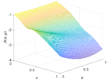
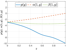
(a) $\alpha_{1}(x,y)$.	(b) $\alpha_{2}(x,y)$.	(c) Control gains $p(t)$, $\alpha_{1}(1,y)$ and $\alpha_{2}(1,y)$.

Figure 2: The numerical solution of kernel function.

5 Finite-time Stability

In this section, we will establish the closed-loop stability. Before discussing the stability, we first give the invertibility of integration transformations; then the equivalence between the target system and the cascaded system is constructed. Finally, the finite-time stability of the closed-loop system is obtained.

First, we present the inverse transformation $(w_{1},w_{2},z)\rightarrow(u_{1},u_{2},v)$, of transformation (4) as follows:

$$u_{1}(x,t)= ~{}w_{1}(x,t)+\int_{0}^{x}L^{11}(x,y)w_{1}(y,t)\,\mathrm{d}y$$

$$~{}+\int_{0}^{x}L^{12}(x,y)w_{2}(y,t)\,\mathrm{d}y,$$ (39a)

$$u_{2}(x,t)= ~{}w_{2}(x,t)+\int_{0}^{x}L^{21}(x,y)w_{1}(y,t)\,\mathrm{d}y$$

$$~{}+\int_{0}^{x}L^{22}(x,y)w_{2}(y,t)\,\mathrm{d}y,$$ (39b)

$$v(x,t)= ~{}z(x,t)+\int_{0}^{x}\mu(x-y)z(y,t)\,\mathrm{d}y$$ (39c)

$$+\int_{0}^{1} \beta_{1}(x,y)w_{1}(y,t)\,\mathrm{d}y+\int_{0}^{1}\beta_{2}(x,y)w_{2}(y,t)\,\mathrm{d}y.$$

Well as the process in Section 3.1, using the integral by parts, we obtain the kernel functions $L^{ij}$, $i,j=1,2$ satisfy a set of hyperbolic PDEs given in [23], and the kernels $\beta_{1}(x,y)$, $\beta_{2}(x,y)$ satisfy:

$$\!\frac{1}{\tau}\partial_{x}\beta_{1}(x,y)+\varepsilon_{1}(y)\partial_{y}\beta_{1}(x,y)= \!-\varepsilon_{1}^{\prime}(y)\beta_{1}(x,y),$$ (40a)

$$\!\frac{1}{\tau}\partial_{x}\beta_{2}(x,y)-\varepsilon_{2}(y)\partial_{y}\beta_{2}(x,y)= ~{}\varepsilon_{2}^{\prime}(y)\beta_{2}(x,y),$$ (40b)

$$\beta_{1}(x,1)= ~{}0,$$ (40c)

$$\varepsilon_{2}(0)\beta_{2}(x,0)= ~{}q\varepsilon_{1}(0)\beta_{1}(x,0),$$ (40d)

$$\beta_{1}(0,y)= ~{}L^{21}(1,y),$$ (40e)

$$\beta_{2}(0,y)= ~{}L^{22}(1,y).$$ (40f)

Then, according to the solution of $\beta_{2}(x,y)$, we get that

$$\mu(x)=\tau\varepsilon_{2}(1)\beta_{2}(x,1).$$ (41)

Second, the stability of target system (5) is established by the following Lemma 3.

Lemma 3.

Consider the system (5) with initial conditions $w_{10}$, $w_{20}$ and $z_{0}\in L^{2}([0,1])$, then the system is finite-time stable, that is, its zero equilibrium is reached in finite-time $t=t_{F}$, where $t_{F}=\tau+\int_{0}^{1}\frac{1}{\varepsilon_{1}(y)}+\frac{1}{\varepsilon_{2}(y)}\,\mathrm{d}y$.

We give the explicit solution of (5) by the method of characteristics as follows,

$$w_{1} =\left\{\begin{aligned} &w_{10}\big{(}\phi_{1}^{-1}[\phi_{1}(x)-t]\big{)},&t\leq\phi_{1}(x),\\ &qw_{2}(0,t-\phi_{1}(x)),&t\textgreater\phi_{1}(x),\end{aligned}\right.$$ (42a)

$$w_{2} =\left\{\begin{aligned} &w_{20}\big{(}\phi_{2}^{-1}[t+\phi_{2}(x)]\big{)},&t\leq\phi_{2}(1)-\phi_{2}(x),\\ &z(0,t+\phi_{2}(x)-\phi_{2}(1)),&t\textgreater\phi_{2}(1)-\phi_{2}(x),\end{aligned}\right.$$ (42b)

$$z =\left\{\begin{aligned} &z_{0}\big{(}x+t/\tau\big{)},&t\leq\tau(1-x),\\ &0,&t\textgreater\tau,\end{aligned}\right.$$ (42c)

which concludes that the target system converges in finite time $t_{F}$ defined in Lemma 3. Thus, this lemma has been proven. Through the above lemmas, the main result of this paper can be obtained as follows:

Theorem 5.2.

Consider the system (3) with the control law (3.1). For any initial condition $u_{10}(x)$, $u_{20}(x)$, $v_{0}(x)\in L^{2}([0,1])$, then the system is finite-time stable, that is, its zero equilibrium is reached in finite-time $t=t_{F}$, where $t_{F}$ is given by Lemma 3.

Note that the finite-time stability of system (1) with control (3.1), which is equivalent to system (3) and (3.1).

6 Robustness analysis

In this section, the delay-robustness is considered. Suppose that $\bar{\tau}=\tau+\Delta\tau>0$ is the uncertain delay which deviates from the true value $\tau$ by $\Delta\tau$. We map cascaded system (3) by transformation (4) to a new system which has same dynamics with (5a)–(5e), except the boundary condition:

$$z(1,t)= ~{}U(t)-\int_{0}^{1}\mu(1-y)z(y,t)\,\mathrm{d}y$$ (43)

$$-\int_{0}^{1}\beta_{1} (1,y)w_{1}(y,t)\,\mathrm{d}y-\int_{0}^{1}\beta_{2}(1,y)w_{2}(y,t)\,\mathrm{d}y,$$

where the inverse transformation (39) is used. Applying the method of characteristics on (5a)–(5e) and (43) yields,

$$w_{1}(x,t)= ~{}qz\left(1,t-\phi_{1}(x)-\phi_{2}(1)-\tau\right),$$ (44a)

$$w_{2}(x,t)= ~{}z\left(1,t-\phi_{2}(1)+\phi_{2}(x)-\tau\right),$$ (44b)

$$z(x,t)= ~{}z(1,t-\tau(1-x)).$$ (44c)

Substituting (44) into (43), we have

$$z(1,t)= ~{}U(t)-\int_{0}^{1}\mu(y)z\left(1,t-\tau y\right)\,\mathrm{d}y$$

$$-\int_{0}^{1} \beta_{1}(1,y)qz\left(1,t-\phi_{1}(y)-\phi_{2}(1)-\tau\right)\,\mathrm{d}y$$

$$-\int_{0}^{1} \beta_{2}(1,y)z\left(1,t-\phi_{2}(1)+\phi_{2}(y)-\tau\right)\,\mathrm{d}y.$$ (45)

Remark 6.3.

If one knows the exact delay $\tau$, then $z(1,t)=0$, which implies the (5a)–(5e) and (43) is a finite-time stable system. However, the exact value of the delay is unknown, so the actual control $U(t)$ adopts $\bar{\tau}$ which deviates from the true delay by a small value $\Delta\tau$. As a result, $z(1,t)$ captures the difference between the actual used control $U(t)$ and the desired control (3.1).

Theorem 6.4.

Consider the control law adopting $\bar{\tau}$:

$$U(t)= ~{}\int_{0}^{1}\bar{p}(1-y)v(y,t)\,\mathrm{d}y+\int_{0}^{1}\bar{\alpha}_{1}(1,y)u_{1}(y,t)\,\mathrm{d}y$$

$$~{}+\int_{0}^{1}\bar{\alpha}_{2}(1,y)u_{2}(y,t)\,\mathrm{d}y,$$ (46)

where the functions $\bar{p}(\cdot)$ and $\bar{\alpha}_{i}(\cdot,\cdot)$, $i=1,2$, are defined in the same way as $p(\cdot)$ and $\alpha_{i}(\cdot,\cdot)$ substituting $\tau$ by $\bar{\tau}$ in (6)–(8). There exist $\Delta\tau_{0}$ such that $|\bar{\tau}-\tau|\leq\Delta\tau_{0}$, the control (6.4) robustly stabilizes the system (3).

Suppose $|\Delta\tau|=|\bar{\tau}-\tau|>0$. The function $\bar{\mu}(\cdot)$ and $\bar{\beta}_{i}(\cdot,\cdot)$, $i=1,2$, are defined by substituting $\bar{\tau}$ for $\tau$ in (40)–(41). Then, use the similar process as (43)–(6) for (6.4), and substitute the result into (6), which gives

$$z(1,t)= \int_{0}^{1}\bar{\mu}(y)z\left(1,t-\bar{\tau}y\right)\,\mathrm{d}y-\int_{0}^{1}\mu(y)z\left(1,t-\tau y\right)\,\mathrm{d}y$$

$$+\int_{0}^{1} \bar{\beta}_{1}(1,y)qz\left(1,t-\phi_{1}(y)-\phi_{2}(1)-\bar{\tau}\right)\,\mathrm{d}y$$

$$-\int_{0}^{1} \beta_{1}(1,y)qz\left(1,t-\phi_{1}(y)-\phi_{2}(1)-\tau\right)\,\mathrm{d}y$$

$$+\int_{0}^{1} \bar{\beta}_{2}(1,y)z\left(1,t-\phi_{2}(1)+\phi_{2}(y)-\bar{\tau}\right)\,\mathrm{d}y$$

$$-\int_{0}^{1} \beta_{2}(1,y)z\left(1,t-\phi_{2}(1)+\phi_{2}(y)-\tau\right)\,\mathrm{d}y.$$ (47)

Taking the Laplace transform of (6), we get characteristic equation $P(s)=1-\sum_{i=1}^{6}H_{i}(s)=0$, $i=1,2,\cdots,6$. The functions $H_{i}(s)$ are defined as,

$$H_{1}(s)= \int_{0}^{1}\mu(y)\mathrm{e}^{-\tau ys}(\mathrm{e}^{-\Delta\tau ys}-1)\,\mathrm{d}y,$$

$$H_{2}(s)= \int_{0}^{1}\Delta\mu(y)\mathrm{e}^{-\bar{\tau}ys}\,\mathrm{d}y,$$

$$H_{3}(s)= \int_{0}^{1}q\beta_{1}(1,y)\mathrm{e}^{-(\phi_{1}(y)+\phi_{2}(1)+\tau)s}(\mathrm{e}^{-\Delta\tau s}-1)\,\mathrm{d}y,$$

$$H_{4}(s)= \int_{0}^{1}q\Delta\beta_{1}(1,y)\mathrm{e}^{-(\phi_{1}(y)+\phi_{2}(1)+\bar{\tau})s}\,\mathrm{d}y,$$

$$H_{5}(s)= \int_{0}^{1}\beta_{2}(1,y)\mathrm{e}^{-(\phi_{2}(1)-\phi_{2}(y)+\tau)s}(\mathrm{e}^{-\Delta\tau s}-1)\,\mathrm{d}y,$$

$$H_{6}(s)= \int_{0}^{1}\Delta\beta_{2}(1,y)\mathrm{e}^{-(\phi_{2}(1)-\phi_{2}(y)+\bar{\tau})s}\,\mathrm{d}y,$$

where $\Delta\mu(y)=\bar{\mu}(u)-\mu(y)$, $\Delta\beta_{1}(1,y)=\bar{\beta}_{1}(1,y)-\beta_{1}(1,y)$ and $\Delta\beta_{2}(1,y)=\bar{\beta}_{2}(1,y)-\beta_{2}(1,y)$. Due to Riemann-Lebesgues’ lemma, we have

$$\forall|s|>M_{0},\quad\int_{0}^{1}\mu(y)\mathrm{e}^{-\tau ys}\,\mathrm{d}y\textless\frac{\xi}{6},$$ (48)

where $\xi\textless 1$. Then, consider the case of $s\leq M_{0}$,

$$|H_{1}(s)|\leq\int_{0}^{1}|\mu(y)|\mathrm{e}^{-\tau ys}(\mathrm{e}^{|\Delta\tau|ys}-1)\ \,\mathrm{d}y.$$ (49)

Since the continuity with respect to $\tau$, we can choose $\Delta\tau\leq\Delta\tau_{0}$ small enough such that (49) less than $\frac{\xi}{6}$. Hence, $\forall s\in\mathbb{C}$, $\forall\Delta\tau\leq\Delta\tau_{0}$, such that $|H_{1}(s)|\textless\frac{\xi}{6}$. Similarly, we have $|H_{3}(s)|\textless\frac{\xi}{6}$ and $|H_{5}(s)|\textless\frac{\xi}{6}$.

Since the continuity of $\mu$, $\beta_{1}$ and $\beta_{2}$, we can choose $\Delta\tau\leq\Delta\tau_{0}$ small enough such that $|H_{2}(s)|\textless\frac{\xi}{6}$, $|H_{4}(s)|\textless\frac{\xi}{6}$ and $|H_{6}(s)|\textless\frac{\xi}{6}$. Consequently, we have

$$|P(s)|\geq 1-\sum_{i=1}^{6}|H_{i}(s)|>0.$$ (50)

It means that for $0<|\Delta\tau|\leq\Delta\tau_{0}$, $P(s)=0$ does not have any roots on the complex right-open plane. As a result, (6) is asymptotically stable, which implies the system (1) with control (3.1) is robust stable due to the invertibility of the transformation (4).

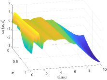
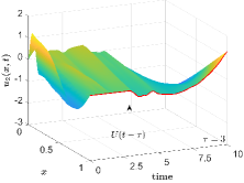
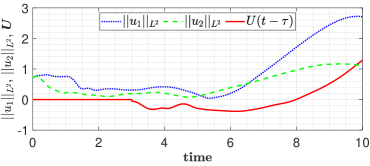
(a) The evolution of $u_{1}$.	(b) The evolution of $u_{2}$.	(c) The $L_{2}$-norm and control effort.
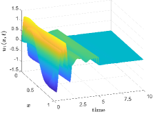
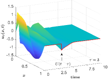
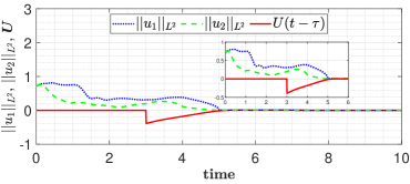
(d) The evolution of $u_{1}$.	(e) The evolution of $u_{2}$.	(f) The $L_{2}$-norm and control effort.

Figure 3: Top (a)–(b): The close-loop response of $2\times 2$ hyperbolic system without delay compensation. Bottom (c)–(d): The response under the delay compensator (3.1).

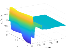
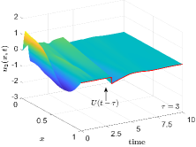
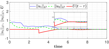
(a) The evolution of $u_{1}$.	(b) The evolution of $u_{2}$.	(c) The $L_{2}$-norm and control effort.

Figure 4: The close-loop response under the delay compensator (3.1) in presence of delay uncertainty, where $\Delta\tau=0.2s$.

7 Simulation

To illustrate Theorem 5.2 and Theorem 6.4, in particular the role played the proposed compensator, the following examples are considered. The parameters in $2\times 2$ first-order system (1) are set as $\varepsilon_{1}=1$, $\varepsilon_{2}=1$, $c_{1}=1$, $c_{2}=1$, $q=1$ and $\tau=3s$. The initial state is set as $u_{10}(x)=\sin(2\pi x)$, $u_{20}(x)=\sin(2\pi x)$. The upwind scheme is employed in MATLAB, where time step $h_{t}=0.01$ and space step $h_{x}=0.01$. The kernel function $K^{ij}(x,y)$ can be solved explicitly using the technique in [39]. Further, the kernel functions $\alpha_{1}(x,y)$, $\alpha_{2}(x,y)$ in (6)–(7) and $p(y)$ in (8) can be solved by using the finite difference method, and their numerical solutions are presented in Fig. 2. In Fig.3(a)–(c), the delayed system evolution under the nominal controller from [22] indicates that a compensator is necessary. It is easy to see that a closed-loop system without delay compensation cannot converge. Meanwhile, the system evolution under the proposed input delay compensator (3.1) is shown in Fig. 3(d)–(e). Through simulation, it was proved that the system controlled by the compensation controller converges to the zero equilibrium in $t_{F}=5s$, which agrees with Theorem 5.2 perfectly. Subsequently, Fig. 4 depicts the evolution of the closed-loop system in presence of an uncertain input delay. The input delay is $\tau=3s$ in the actual system, but the parameter used in the compensator with delay variation $\Delta\tau=0.2s$. As expected in Theorem 6.4, the closed-loop system is robustly stable.

8 Conclusion

In this paper, we propose a backstepping-based input-delay-compensated boundary controller to stabilize a $2\times 2$ hyperbolic system subject to an uncertain input delay. The well-posedness of the kernel function is explored using the method of characteristics and successive approximation method. Therefore, under the action of the proposed compensator, the finite-time stability of the hyperbolic system are guaranteed. Moreover, the robustness of the proposed controller is analyzed using the equivalent neutral equation. Future research issues are to consider compensation control design with non-constant delays, such as spatial- or time-varying delays, or to consider the time-delay compensation problem for more general $m+n$ hyperbolic system.

References

- [1] G. Q. Xu, S. P. Yung, L. K. Li, Stabilization of wave systems with input delay in the boundary control, ESAIM: Control, Optimisation and Calculus of Variations 12 (4) (2006) 770–785.
- [2] H. Lhachemi, C. Prieur, R. Shorten, Robustness of constant-delay predictor feedback for in-domain stabilization of reaction–diffusion PDEs with time-and spatially-varying input delays, Automatica 123 (2021) 109347.
- [3] M. Krstic, A. Smyshlyaev, Backstepping boundary control for first-order hyperbolic PDEs and application to systems with actuator and sensor delays, Systems Control Letters 57 (9) (2008) 750–758.
- [4] A. Braik, A. Beniani, Y. Miloudi, Well-posedness and general decay of solutions for the heat equation with a time varying delay term, Kragujevac Journal of Mathematics 46 (2) (2022) 267–282.
- [5] C. Prieur, F. Mazenc, ISS-Lyapunov functions for time-varying hyperbolic systems of balance laws, Mathematics of Control, Signals, and Systems 24 (1) (2012) 111–134.
- [6] K. Ding, Q. Zhu, Fuzzy intermittent extended dissipative control for delayed distributed parameter systems with stochastic disturbance: a spatial point sampling approach, IEEE Transactions on Fuzzy Systems 30 (6) (2021) 1734–1749.
- [7] D. Khusainov, M. Pokojovy, R. Racke, Strong and mild extrapolated -solutions to the heat equation with constant delay, SIAM Journal on Mathematical Analysis 47 (1) (2015) 427–454.
- [8] M. Krstic, Delay compensation for nonlinear, adaptive, and PDE systems, Springer, 2009.
- [9] J. Zhang, J. Qi, Compensation of spatially-varying state delay for a first-order hyperbolic PIDE using boundary control, Systems Control Letters 157 (2021) 105050.
- [10] M. Krstic, Control of an unstable reaction–diffusion PDE with long input delay, Systems Control Letters 58 (10) (2009) 773–782.
- [11] J. Qi, M. Krstic, Compensation of spatially varying input delay in distributed control of reaction-diffusion PDEs, IEEE Transactions on Automatic Control 66 (9) (2020) 4069–4083.
- [12] J. Qi, S. Wang, J.-A. Fang, M. Diagne, Control of multi-agent systems with input delay via PDE-based method, Automatica 106 (2019) 91–100.
- [13] G. Freudenthaler, T. Meurer, PDE-based multi-agent formation control using flatness and backstepping: Analysis, design and robot experiments, Automatica 115 (2020) 108897.
- [14] H. Anfinsen, O. M. Aamo, Adaptive output feedback stabilization of coupled linear hyperbolic PDEs with uncertain boundary conditions, SIAM Journal on Control and Optimization 55 (6) (2017) 3928–3946.
- [15] S. Wang, M. Diagne, J. Qi, Delay-adaptive predictor feedback control of reaction-advection-diffusion PDEs with a delayed distributed input, IEEE Transactions on Automatic Control 67 (7) (2022) 3762–3769.
- [16] J. Deutscher, A backstepping approach to the output regulation of boundary controlled parabolic PDEs, Automatica 57 (2015) 56–64.
- [17] J. Zhang, J. Qi, S. Dubljevic, B. Shen, Output regulation for a first-order hyperbolic PIDE with state and sensor delays, European Journal of Control 65 (2022) 100643.
- [18] R. M. Colombo, A hyperbolic traffic flow model, Mathematical and computer modelling 35 (5-6) (2002) 683–688.
- [19] V. Dos Santos, C. Prieur, Boundary control of open channels with numerical and experimental validations, IEEE transactions on Control systems technology 16 (6) (2008) 1252–1264.
- [20] G. Bastin, J.-M. Coron, On boundary feedback stabilization of non-uniform linear hyperbolic systems over a bounded interval, Systems Control Letters 60 (11) (2011) 900–906.
- [21] O. M. Aamo, Leak detection, size estimation and localization in pipe flows, IEEE Transactions on Automatic Control 61 (1) (2015) 246–251.
- [22] R. Vazquez, M. Krstic, J.-M. Coron, Backstepping boundary stabilization and state estimation of a linear hyperbolic system, in: 2011 50th IEEE conference on decision and control and european control conference, IEEE, 2011, pp. 4937–4942.
- [23] J.-M. Coron, R. Vazquez, M. Krstic, G. Bastin, Local exponential stabilization of a quasilinear hyperbolic system using backstepping, SIAM Journal on Control and Oprimization 51 (3) (2013) 2005–2035.
- [24] F. Di Meglio, R. Vazquez, M. Krstic, Stabilization of a system of coupled first-order hyperbolic linear PDEs with a single boundary input, IEEE Transactions on Automatic Control 58 (12) (2013) 3097–3111.
- [25] L. Hu, F. Di Meglio, R. Vazquez, M. Krstic, Control of homodirectional and general heterodirectional linear coupled hyperbolic PDEs, IEEE Transactions on Automatic Control 61 (11) (2016) 3301–3314.
- [26] S. Tang, B.-Z. Guo, M. Krstic, Active disturbance rejection control for a hyperbolic system with an input disturbance, IFAC Proceedings Volumes 47 (3) (2014) 11385–11390.
- [27] H. Anfinsen, O. M. Aamo, Disturbance rejection in the interior domain of linear hyperbolic systems, IEEE Transactions on Automatic Control 60 (1) (2014) 186–191.
- [28] A. Irscheid, N. Gehring, J. Deutscher, J. Rudolph, Observer design for linear hyperbolic PDEs that are bidirectionally coupled with nonlinear ODEs, in: 2021 European Control Conference (ECC), IEEE, 2021, pp. 2506–2511.
- [29] J. Wang, M. Krstic, Delay-compensated event-triggered boundary control of hyperbolic PDEs for deep-sea construction, Automatica 138 (2022) 110137.
- [30] J. Auriol, U. J. F. Aarsnes, P. Martin, F. Di Meglio, Delay-robust control design for two heterodirectional linear coupled hyperbolic PDEs, IEEE Transactions on Automatic Control 63 (10) (2018) 3551–3557.
- [31] J. Auriol, F. Di Meglio, An explicit mapping from linear first order hyperbolic PDEs to difference systems, Systems Control Letters 123 (2019) 144–150.
- [32] J. Auriol, Output feedback stabilization of an underactuated cascade network of interconnected linear PDE systems using a backstepping approach, Automatica 117 (2020) 108964.
- [33] J. Auriol, D. B. Pietri, Robust state-feedback stabilization of an underactuated network of interconnected n+m hyperbolic PDE systems, Automatica 136 (2022) 110040.
- [34] J. Auriol, F. Bribiesca-Argomedo, S.-I. Niculescu, J. Redaud, Stabilization of a hyperbolic PDEs–ODE network using a recursive dynamics interconnection framework, in: 2021 European control conference (ECC), IEEE, 2021, pp. 2493–2499.
- [35] J. Redaud, J. Auriol, S.-I. Niculescu, Output-feedback control of an underactuated network of interconnected hyperbolic PDE–ODE systems, Systems Control Letters 154 (2021) 104984.
- [36] H. Anfinsen, O. M. Aamo, Adaptive output-feedback stabilization of linear hyperbolic PDEs with actuator and sensor delay, in: 2018 26th Mediterranean Conference on Control and Automation (MED), IEEE, 2018, pp. 1–6.
- [37] I. Karafyllis, M. Krstic, On the relation of delay equations to first-order hyperbolic partial differential equations, ESAIM: Control, Optimisation and Calculus of Variations 20 (3) (2014) 894–923.
- [38] M. Krstic, A. Smyshlyaev, Boundary control of PDEs: A course on backstepping designs, SIAM, 2008.
- [39] R. Vazquez, M. Krstic, Marcum Q-functions and explicit kernels for stabilization of linear hyperbolic systems with constant coefficients, Systems Control Letters 68 (2014) 33–42.