Attention to Entropic Communication

Abstract

The concept of attention, numerical weights that emphasize the importance of particular data, has proven to be very relevant in artificial intelligence. Relative entropy (RE, aka Kullback-Leibler divergence) plays a central role in communication theory. Here we combine these concepts, attention and RE. RE guides optimal encoding of messages in bandwidth-limited communication as well as optimal message decoding via the maximum entropy principle (MEP). In the coding scenario, RE can be derived from four requirements, namely being analytical, local, proper, and calibrated. Weighted RE, used for attention steering in communications, turns out to be improper. To see how proper attention communication can emerge, we analyze a scenario of a message sender who wants to ensure that the receiver of the message can perform well-informed actions. If the receiver decodes the message using the MEP, the sender only needs to know the receiver’s utility function to inform optimally, but not the receiver’s initial knowledge state. In case only the curvature of the utility function maxima are known, it becomes desirable to accurately communicate an attention function, in this case a by this curvature weighted and re-normalized probability function. Entropic attention communication is here proposed as the desired generalization of entropic communication that permits weighting while being proper, thereby aiding the design of optimal communication protocols in technical applications and helping to understand human communication. For example, our analysis shows how to derive the level of cooperation expected under misaligned interests of otherwise honest communication partners. Key words: information theory; communication theory; entropy; attention; weighted Kullback Leibler Divergence

1 Introduction

1.1 Relative Entropy

The work of Shannon [1] and Jaynes [2, 3, 4, 5, 6] made it clear that entropy and its generalizations [7, 8, 9], in particular to relative entropy [10], have a root in communication theory. Already introduced by [11] in 1906 to thermodynamics, relative entropy plays nowadays a central role in artificial intelligence [12, 13, 14, 15, 16], particularly for variational autoencoder [17, 18, 19, 20], as well as in information field theory [21, 22, 23]. Relative entropy permits to code maximal informative messages and the Maximum Entropy Principle (MEP) [2, 3, 4, 5, 6] to decode such, as detailed in the following.

The relative entropy between two probability densities $\mathcal{P}(s|I_{\text{A}})$ and $\mathcal{P}(s|I_{\text{B}})$ on an unknown signal or situation $s\in\mathcal{S}$

$$\mathcal{D}_{s}(I_{\text{A}},I_{\text{B}}) := \int_{\mathcal{S}}ds\,\mathcal{P}(s|I_{\text{A}})\,\ln\frac{\mathcal{P}(s|I_{\text{A}})}{\mathcal{P}(s|I_{\text{B}})}$$ (1)

measures the amount of information in nits lost by degrading some knowledge $I_{\text{A}}$ to knowledge $I_{\text{B}}$. The letters A and B stand for Alice and Bob, who are communication partners. Alice can use the relative entropy to decide which message she wants to send to Bob in order to inform him best. $I_{\text{A}}$ is Alice’s background information before and after her communication.

We assume that Alice knows how to communicate such that Bob updates his previous knowledge state $I_{0}$ to $I_{\text{B}}$.

The functional form of the relative entropy can be derived from various lines of argumentation [27, 28, 29, 30, 31, 32]. As the most natural information measure relative entropy plays a central role in information theory. It is often used as the quantity to be minimized when deciding which of the possible messages shall be sent through a bandwidth limited communication channel that does not permit the full transfer of $I_{\text{A}}$, but also in other circumstances.

As we will discuss in more detail, relative entropy as specified by Eq. 1 is uniquely determined up to a multiplicative factor as the measure to determine the optimal message to be sent under the requirements of it being analytical (all derivatives w.r.t. to the parameters in $I_{\text{B}}$ exist everywhere), local (only the $s$ that happens will matter in the end), proper (to favor $I_{\text{B}}=I_{\text{A}}$) [33, 34, 8], and calibrated (being zero when $I_{\text{B}}=I_{\text{A}}$). Our derivation is a slight modification of that given in [30].

A number of attempts have been made to introduce weights into the relative entropy [35, 36, 32, 37, 38, 39, 40]. Some of these go back to [41, 42]. Most of them can be summarized by the weighted relative entropy,

$$\mathcal{\widetilde{D}}_{s}^{(w)}(I_{\text{A}},I_{\text{B}}) := \int_{\mathcal{S}}ds\,w(s)\,\mathcal{P}(s|I_{\text{A}})\,\ln\frac{\mathcal{P}(s|I_{\text{A}})}{\mathcal{P}(s|I_{\text{B}})},$$ (2)

with weights $w(s)$, for which $w(s)\geq 0$ holds for all $s\in\mathcal{S}$.

The extension of relative entropy to weighted relative entropy, as given by Eq. 2, appears to be attractive, as it can reflect scenarios in which not all possibilities in $\mathcal{S}$ are equally important. For example, detailed knowledge on the subset of situations $\mathcal{S}_{\text{B dead}}\subset\mathcal{S}$ in which Bob’s decisions do not matter to him are not very relevant for the communication, as he can not gain much practical use from it. Therefore, Alice should not waste valuable communication bandwidth for details within $\mathcal{S}_{\text{B dead}}$, but use it to inform him about the remaining situations $\mathcal{S}_{\text{B alive}}=\mathcal{S}\backslash\mathcal{S}_{\text{B dead}}$ for which being well informed makes a difference to Bob. However, despite being well motivated, weighted relative entropy is not proper in the mathematical sense for non-constant weighting functions, as we will show and was already recognized before [32].

1.2 Relative Attention Entropy

Given the success of attention weighting in artificial intelligence research [43, 44, 45], in particular in transformer networks [45], the question arises whether a form of weighted relative entropy exists that is proper. In order to understand how the weighting should be included we investigate a specific communication scenario, in which weighted and re-normalized probabilities of the form

$$\mathcal{A}^{(w)}(s|I):=\frac{w(s)\,\mathcal{P}(s|I)}{\int_{\mathcal{S}}ds^{\prime}\,w(s^{\prime})\,\mathcal{P}(s^{\prime}|I)}$$ (3)

appear naturally as the central element of communication. We will call a quantity of this form attention function, attention density function, or briefly attention when there is no risk of confusion with other attention concepts (as within this paper).

The corresponding relative attention entropy

$$\mathcal{D}_{s}^{(w)}(I_{\text{A}},I_{\text{B}}) \negmedspace\!:=\negmedspace\! \int_{\mathcal{S}}ds\,\mathcal{A}^{(w)}(s|I_{\text{A}})\,\ln\frac{\mathcal{A}^{(w)}(s|I_{\text{A}})}{\mathcal{A}^{(w)}(s|I_{\text{B}})},$$ (4)

leads to proper communication, in case $w(s)>0$ for all $s\in\mathcal{S}$, as we show in the following. The minimum of the relative attention entropy is given by $\mathcal{A}^{(w)}(s|I_{\text{B}})=\mathcal{A}^{(w)}(s|I_{\text{A}})$, which in case $w(s)>0$ for all $s\in\mathcal{S}$ implies $\mathcal{P}(s|I_{\text{B}})=\mathcal{P}(s|I_{\text{A}})$ since

$$\mathcal{P}(s|I_{\text{B}}) = \frac{\mathcal{A}^{(w)}(s|I_{\text{B}})/w(s)}{\int_{\mathcal{S}}ds^{\prime}\,\mathcal{A}^{(w)}(s^{\prime}|I_{\text{B}})/w(s^{\prime})}$$ (5)

$$= \frac{\mathcal{A}^{(w)}(s|I_{\text{A}})/w(s)}{\int_{\mathcal{S}}ds^{\prime}\,\mathcal{A}^{(w)}(s^{\prime}|I_{\text{A}})/w(s^{\prime})}$$

$$= \frac{\mathcal{P}^{(w)}(s|I_{\text{A}})/\int_{\mathcal{S}}ds\,w(s^{\prime\prime})\mathcal{\,P}(s^{\prime\prime}|I_{\text{A}})}{\int_{\mathcal{S}}ds\,\mathcal{P}^{(w)}(s^{\prime}|I_{\text{A}})/\int_{\mathcal{S}}ds\,w(s^{\prime\prime\prime})\mathcal{\,P}(s^{\prime\prime\prime}|I_{\text{A}})}$$

$$= \mathcal{P}(s|I_{\text{A}}).$$

Here we first turned the attention back into a probability by inversely weighting and re-normalization, then substituted $\mathcal{A}^{(w)}(s|I_{\text{B}})$ by $\mathcal{A}^{(w)}(s|I_{\text{A}})$ thanks to their identity, further substituted the latter by its definition in terms of $\mathcal{P}(s|I_{\text{A}})$, and finally used the normalization $\int_{\mathcal{S}}ds\,\mathcal{P}(s|I_{\text{A}})=1$.

The relative attention entropy differs from weighted relative entropy (Eq. 2) due to the re-normalization in the definition of attention, which leads to an irrelevant re-scaling of weighted relative entropy, since independent of $I_{\text{B}}$, but also to a relevant extra term that depends on $I_{\text{B}}$:

$$\mathcal{D}_{s}^{(w)}(I_{\text{A}},I_{\text{B}}) \negmedspace\!\negmedspace\!\negmedspace\!\negmedspace\!=\negmedspace\!\negmedspace\!\negmedspace\!\negmedspace\! \frac{\mathcal{\widetilde{D}}_{s}^{(w)}(I_{\text{A}},I_{\text{B}})-\!\ln\frac{\int_{\mathcal{S}}\!ds\,w(s)\,\mathcal{P}(s|I_{\text{A}})}{\int_{\mathcal{S}}\!ds\,w(s)\,\mathcal{P}(s|I_{\text{B}})}}{\int_{\mathcal{S}}\!ds\,w(s)\,\mathcal{P}(s|I_{\text{A}})}\!$$

This extra term ensures properness when the attention entropy gets minimized w.r.t. $I_{\text{B}}$. We refrained here to give similar integration variables different names.

We investigate the specific scenario of Alice wanting to inform Bob optimally. From this, we will motivate attention according to Eq. 4. This means that she wants to prepare Bob such that he can decide about an action $a\in\mathbb{A}$ in a for him optimal way. This action has an outcome for Bob that depends on the unknown situation $s$ Alice tries to inform Bob about. The outcome is described by a utility function $u(s,a)$, which both, Alice and Bob want to maximize. The utility depends on both, the unknown situation $s$ and Bob’s action $a$. In the following, we assume $u(s,a)$ to be at least twice differentiable w.r.t. $a$ and to exhibit only one maxima for any given $s.$ In case Alice does not know Bob’s utility function, but its curvature w.r.t. $a$ at its maxima for any given $s$, it will turn out that Alice wants to communicate her attention $\mathcal{A}^{(w)}(s|I_{\text{A}})$ as accurately as possible to Bob, where $w(s)$ is the curvature of the utility w.r.t. $a$. In short, we will show that Alice should inform Bob most precisely about situations in which Bob’s decision requires the largest accuracy and not at all about situations in which his actions do not make any difference. The functional, according to which Alice will fit $I_{\text{B}}$ to $I_{\text{A}}$, will not be the relative attention entropy of Eq. 4, but a different one. However, it motivates attention as an essential element of utility aware communication and shows the path to extend the derivation of relative entropy to that of relative attention entropy.

1.3 Attention Example

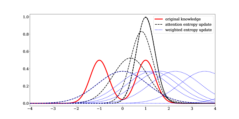
Figure 1: Example of communication based on relative attention entropy and weighted relative entropy as discussed in Sect. 1.3. Alice’s bimodal knowledge state is given by the red solid curve. Bob’s final knowledge state after Alice’s communication is shown for various cases. The dashed black lines correspond to cases in which Alice uses relative attention entropy, and the dotted blue lines to cases she uses weighted relative entropy. Different results for the weight function $w(s)=\exp(\lambda\,s)$ with $\lambda=0$, $1$, $2$, $4,$ $8$, $16$, and $32$ are shown from left two right, respectively. In case $\lambda=0$ relative entropy, relative attention entropy, and weighted relative entropy give the same result, the shown zero centered Gaussian. For $\lambda\geq 8$ the different curves for the relative attention entropy results are visually indistinguishable and indicate the result of the $\lambda\rightarrow\infty$ limit.

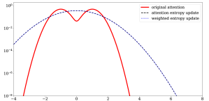
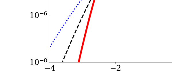
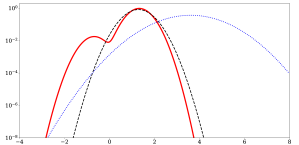
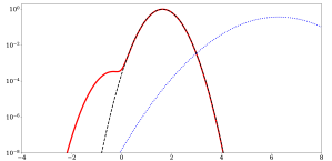
Figure 2: Attention functions corresponding to the cases $\lambda=0,\text{ }1,\text{ }2,\text{ and }4$ of Fig. 1 on logarithmic scale to display the unattended peak of the Alice’s attention. Note that due to the strong exponential focus of the weights on larger $s$-values the attention peaks are displaced to the right w.r.t. the corresponding knowledge peaks.

To illustrate how relative attention entropy works in practice, we investigate an illustrative example. For this we assume that Alice has a bimodal knowledge state

$$\mathcal{P}(s|I_{\text{A}})=\frac{1}{2}\sum_{x\in\{-1,1\}}\mathcal{G}\left(s-x,\sigma_{\text{A}}^{2}\right)$$ (7)

on a situation $s$ about which she wants to inform Bob, which is a superposition of two Gaussians, with

$$\mathcal{G}(s,\sigma^{2}):=\frac{1}{\sqrt{2\pi\sigma^{2}}}\exp\left(-\frac{s^{2}}{2\sigma^{2}}\right).$$ (8)

This is shown in Fig. 1.

Let us assume that Alice believes that the different situations have importance weights $w(s)=e^{\lambda\,s}$ for Bob, with $\lambda$ controlling the inhomogeneity of the weights. We further assume that her communication can only create Gaussian knowledge states in Bob of the form

$$\mathcal{P}(s|I_{\text{B}})=\mathcal{G}\left(s-m,\sigma_{\text{B}}^{2}\right).$$ (9)

The corresponding attentions of Alice and Bob are

$$\mathcal{A}^{(w)}(s|I_{\text{A}}) = \!\negmedspace\!\!\sum_{x\in\{-1,1\}}\negmedspace\!\negmedspace\!\frac{e^{x\,\lambda}\mathcal{G}\left(s-x-\lambda\sigma_{\text{A}}^{2},\sigma_{\text{A}}^{2}\right)}{2\,\cosh\lambda},$$ (10)

$$\mathcal{A}^{(w)}(s|I_{\text{B}}) = \mathcal{G}\left(s-m-\lambda\sigma_{\text{B}}^{2},\sigma_{\text{B}}^{2}\right),$$ (11)

respectively, as shown in App. A, which also covers the details of the following calculations. These functions are displayed in Fig. 2 for smaller values of $\lambda$.

Matching the parameters $m$ and $\sigma_{\text{B}}^{2}$ by minimizing the relative attention entropy in Eq. 4 w.r.t.  those yield

$$m = \tanh\lambda-\frac{\lambda}{\cosh^{2}\lambda},$$ (12)

$$\sigma_{\text{B}}^{2} = \sigma_{\text{A}}^{2}+1-\tanh^{2}\lambda.$$ (13)

The resulting communicated attention weighted knowledge is depicted in Fig. 1 for various values of $\lambda$. The case $\lambda=0$ corresponds to homogeneous weights and therefore to using the non-weighted relative entropy, Eq. 1. In this case Alice communicates a broad knowledge state to Bob that covers both peaks of her knowledge. With increasing $\lambda$ the right peak becomes more important and Alice puts more and more attention on communicating its location and shape more accurately. In the limit of $\lambda\rightarrow\infty$ we have $m=1$ and $\sigma_{\text{B}}^{2}=\sigma_{\text{A}}^{2}$, meaning that Alice communicates exactly this relevant peak at $s=+1$ and completely ignores the for Bob irrelevant one at $s=-1$.

Minimizing the weighted entropy of Eq. 2 instead, yields $\mathcal{P}(s|\widetilde{I_{B}})=\mathcal{G}(s-\widetilde{m},\widetilde{\sigma}_{\text{B}}^{2})$ with

$$\widetilde{m} = \lambda\,\sigma_{\text{A}}^{2}+\tanh\lambda$$ (14)

$$\widetilde{\sigma}_{\text{B}}^{2} = \sigma_{\text{A}}^{2}+1,$$ (15)

which results in poorly adapted communicated knowledge states, as also depicted in Fig. 1. Weighted relative entropy just moves the broad peak centered originally at zero for both entropies in case of no weight ($\lambda=0$) to increasingly more extreme locations, which for $\lambda\rightarrow\infty$ become completely detached from the location of the relevant peak. This detachment is clearly visible in Fig. 1 and Fig. 2.

In order to see how the process of Alice informing Bob works in detail, we have to understand how he decodes messages, as this defines the format of the messages Alice can send. The best way for him to incorporate knowledge sent to him into his own beliefs is by using the MEP, which we assume he does in the following.

1.4 Maximum Entropy Principle

The MEP was derived as a device to optimally decode messages and to incorporate their information into preexisting knowledge [2, 3, 4, 5, 6, 48]. The MEP states that among all possible updated probability distributions that are consistent with the message, the one with the largest entropy should be taken. Requiring that this update should be local, reparametrization invariant (w.r.t. the way the signal or situation $s\in\mathcal{S}$ is expressed), and separable (w.r.t. handling independent dimensions of $s$) enforces the functional form (up to affine transformations) of this entropy to be

$$D_{s}(I_{\text{B}},I_{0})=\int_{\mathcal{S}}ds\,\mathcal{P}(s|I_{\text{B}})\,\ln\frac{\mathcal{P}(s|I_{\text{B}})}{\mathcal{P}(s|I_{0})}$$ (16)

with $I_{0}$ being Bob’s knowledge before and $I_{\text{B}}$ after the update.

We assume that Alice’s message takes the form

$$``\langle f(s)\rangle_{(s|I_{A})}=d".$$ (17)

We call the function $f:\mathcal{S}\rightarrow\mathbb{R}^{n}$ the topic of the communication, as it expresses the specific aspects of $s$ that Alice’s message is about. E.g. in case Alice wants to inform Bob about the first moment of the first component of $s\in\mathbb{R}^{n}$, the topic would be $f(s)=s_{1}$. As Alice communicates it, the topic is known to both, Alice and Bob. Here, $\langle f(s)\rangle_{(s|I_{A})}:=\int_{\mathcal{S}}ds\,f(s)\,\mathcal{P}(s|I_{\text{A}})$ is a compact notation for evaluating this topic as an expectation value. The communicated expectation value of $f$ is called in the following the message data $d$. The word data expresses that a quantity can be regarded as a certain fact, which still might have an uncertain interpretation. In this case it is certain to Bob that Alice claims that $\langle f(s)\rangle_{(s|I_{A})}$ has the value $d$. Under the premise that Alice is honest, this informs Bob about her belief, and if he can assume further that she is also well informed, the data is informative on $s$ itself. Under the premise that Alice is dishonest, $d$ could still inform Bob about what she wants him to believe, and therefore still be data, just on Alice’s intentions and not on her knowledge.

Alice’s message $m$ to Bob therefore consists of the tuple $(f,d).$ Although this message construction might look artificial at a first glance, it actually can express many, if not all real world communications, as we motivate in App. B.

Updating his knowledge according to the MEP after receiving the message implies that Bob extremizes the constrained entropy

$$\!\!\!\!\!\mathcal{E}_{s}(I_{\text{B}},\mu|I_{0},m) \!\!\!\!\!:=\!\!\!\!\! \mathcal{D}_{s}(I_{\text{B}},I_{0})+\mu^{\text{t}}\left(\langle f(s)\rangle_{(s|I_{B})}-d\right)$$ (18)

w.r.t. the arguments $I_{\text{B}}$ and $\mu$. Here, the latter is a Lagrange multiplier that ensures that Alice’s statement, Eq. 17, is imprinted onto Bob’s knowledge $\mathcal{P}(s|I_{\text{B}})$. The MEP and the requirement of normalized probabilities then imply that Bob’s updated knowledge is of the form

$$\mathcal{P}(s|I_{\text{B}}) = \frac{\mathcal{P}(s|I_{0})\,\exp\left(\mu^{\text{t}}f(s)\right)}{\mathcal{Z}(\mu,f)}\text{, with}$$ (19)

$$\mathcal{Z}(\mu,f) := \int\text{d}s\,\mathcal{P}(s|I_{0})\,\exp\left(\mu^{\text{t}}f(s)\right).$$ (20)

The Lagrange multiplier $\mu$ needs to be chosen such that $\langle f(s)\rangle_{(s|I_{\text{B}})}=d$, which can be achieved by requiring

$$\frac{\partial\ln\mathcal{Z}(\mu,f)}{\partial\mu}=d,$$ (21)

since

$$\frac{\partial\ln\mathcal{Z}(\mu,f)}{\partial\mu} = \frac{1}{\mathcal{Z}(\mu,f)}\frac{\partial\mathcal{Z}(\mu,f)}{\partial\mu}$$ (22)

$$= \frac{1}{\mathcal{Z}(\mu,f)}\int\text{d}s\,q(s)\,\exp\left(\mu^{\text{t}}f(s)\right)$$

$$= \langle f(s)\rangle_{(s|I_{\text{B}})}.$$

Thus, the MEP procedure ensures that the communicated moment of Alice’s knowledge state, $\langle f(s)\rangle_{(s|I_{\text{A}})}=d$, gets transferred accurately into Bob’s knowledge,

$$\langle f(s)\rangle_{(s|I_{\text{A}})}=\langle f(s)\rangle_{(s|I_{\text{B}})},$$ (23)

and thus that Bob extracts all information Alice has sent to him. Alice’s communicated expectation for the topic, $d=\langle f(s)\rangle_{(s|I_{\text{A}})}$, is now “imprinted” onto Bob’s knowledge, as $\langle f(s)\rangle_{(s|I_{\text{B}})}=d$ as well after his update.

If Bob decodes Alice’s message via the MEP, she can send a perfectly accurate image of her knowledge if the communication channel bandwidth permits for this. Detailed explanations on this can be found in App. C. Otherwise, she needs to compromise and for this requires a criterion on how to do so.

The protocol of the entropy-based communication between Alice and Bob looks therefore as follows:

Both know:

The situation/signal $s$ is in a set $\mathcal{S}$ of possibilities, on which they have information $I_{\text{A}}$ and $I_{0}$, respectively, implying for each a knowledge state $\mathcal{P}(s|I_{\text{A}})$ and $\mathcal{P}(s|I_{0})$, respectively.

Alice sends:

A function $f:\mathcal{S}\rightarrow\mathbb{R}^{n}$, the message topic, and her expectation for it, $d=\langle f(s)\rangle_{P(s|I_{\text{A}})}$, the message data.

Bob updates:

$I_{0}\rightarrow I{}_{\text{B}}$, according to the MEP, such that his updated knowledge $\mathcal{P}(s|I_{\text{B}})$ has the same expectation value w.r.t. the topic, $d=\langle f(s)\rangle_{P(s|I_{\text{B}})}$.

1.5 Structure of this Work

The remainder of this work is structured as follows. Sect. 2 recapitulates the derivation of relative entropy by [27, 30] and shows that a non-trivially weighted relative entropy is not proper. Sect. 3 then discusses variants of our communication scenario in which Alice’s and Bob’s utility functions are known to them, be them aligned or misaligned. In Sect. 4 we show that attention emerges as the quantity to be communicated most accurately in case Alice wants the best for Bob, but lack’s precise knowledge on Bob’s utility except for its curvature w.r.t  Bob’s action in any situation. This motivates the introduction of attention to entropic communication. In Sect. 5 relative attention entropy is derived in analogy to the derivation of relative entropy. We conclude in Sect. 6 with discussing the relevance of our analysis in technological and socio-psychological contexts.

2 Proper and Weighted Coding

2.1 Proper Coding

In order to see the relation of being proper and relative entropy, we recapitulate its derivation as given by [30] in a modified way. There, it was postulated that Alice uses a loss function $\mathcal{L}(s,I_{\text{A}},I_{\text{B}})$ (negative utility) that depends on the situation $s$ that happens in the end, as well as her and Bob’s knowledge at this point, $I_{\text{A}}$ and $I_{\text{B}}$, respectively. [30] call this function her embarrassment, as it should encode how badly she informed Bob about the situation $s$ that happens in the end. Obviously, Alice wants to minimize this embarrassment.

At the time Alice has to make her choice, she does not know which situation $s=s_{*}$ will happen. She therefore needs to minimize her expected loss

$$\mathcal{L}(I_{\text{A}},I_{\text{B}}) := \left\langle\mathcal{L}(s_{*},I_{\text{A}},I_{\text{B}})\right\rangle_{(s_{*}|I_{\text{A}})}$$ (24)

for deciding which knowledge state Bob $I_{\text{B}}$ should get (via her message $m$). Here we discriminate the related, but different functions labeled by $\mathcal{L}$ via their signatures (their sets of arguments).

General criteria such a loss function should obey were formulated by [30], which we slightly rephrase here as:

Analytical:

Alice’s loss should be an analytic expression of its arguments. An analytic function is an infinitely differentiable function such that it has a converging Taylor series in a neighborhood of any point of its domain. As a consequence, an analytical function is fully determined for all locations of its domain (assuming this is connected) by such a Taylor series around any of the domain positions.

Locality:

In the end, only the case that happens matters. Without loss of generality, let’s assume that $s=s_{*}$ turned out to be the case. Of all statements about $s$, only her prediction $\mathcal{P}(s_{*}|I_{\text{B}})$ that Alice made about $s_{*}$ before $s_{*}$ turned out to be the case, is relevant for her loss.

Properness:

If possible, Alice should favor to transmit her actual knowledge state to Bob, $I_{\text{B}}=I_{\text{A}}$.

Calibration:

The expected loss of being proper shall be zero.

1. Locality implies that $\mathcal{L}(s,I_{\text{A}},I_{\text{B}})$ can only depend on $I_{\text{A}}$ and $I_{\text{B}}$ through $q(s):=\mathcal{P}(s|I_{\text{B}})$ and $p(s):=\mathcal{P}(s|I_{\text{A}})$, meaning

   $$\mathcal{L}(s,I_{\text{A}},I_{\text{B}})=\mathcal{L}(s,p(s),q(s))+\lambda\,\left(1-\int\text{d}s^{\prime}\,q(s^{\prime})\right),$$ (25)

   again using the function signatures to discriminate different $\mathcal{L}^{\prime}$s and introducing a Lagrange multiplier to ensure that $\mathcal{P}(s|I_{\text{B}})$ is normalized.

Properness then requests that the expected loss should be minimal for $q=p$, implying for all possible $s=s_{*}$

$$0 = \left.\frac{\partial\mathcal{L}(I_{\text{A}},I_{\text{B}})}{\partial q(s_{*})}\right|_{q=p}$$ (26)

$$= \frac{\partial}{\partial q(s_{*})}\times$$

$$\left.\left\langle\mathcal{L}(s,p(s),q(s))-\lambda\,\int\text{d}s^{\prime}\,q(s^{\prime})\right\rangle_{(s|I_{\text{A}})}\right|_{q=p}$$

$$= \left.\int\text{d}s\,\delta(s-s_{*})\left[\frac{\partial\mathcal{L}(s,p(s),y)}{\partial y}\right]_{y=q(s)}\!\!\!\!\mathcal{P}(s|I_{\text{A}})\right|_{q=p}\!\!\!\!-\lambda$$

$$= \left.\left[\frac{\partial\mathcal{L}(s,p(s_{*}),y)}{\partial y}\right]_{y=q(s_{*})}\!\!\!\!p(s_{*})\right|_{q=p}\!\!\!\!-\lambda$$

$$= \left.\left[\frac{\partial\mathcal{L}(s,x,y)}{\partial y}\right]_{y=x}x-\lambda\right|_{x=q(s_{*})}.$$

From this

$$\left[\frac{\partial\mathcal{L}(s,x,y)}{\partial y}\right]_{y=x}=\frac{\lambda}{x}$$ (27)

follows, which is solved analytically by

$$\mathcal{L}(s,x,y)=\lambda\,\ln\,y+c(s,x),$$ (28)

as can be verified by insertion. The Lagrange multiplier is unspecified and we choose it to be $\lambda=1$, with the positive sign of $\lambda$ ensuring that $\mathcal{L}$ is actually a minimum and the magnitude $|\lambda|=1$ that the units of this loss are nits ($\lambda=1/\ln 2$ would set the units to bits or shannons).

Calibration requests then that $0=\mathcal{L}(s,x,x)=\ln\,x+c(s,x)$, therefore $c(s,x)=-\ln x$, and thus, by reinsertion this into Eq. 24, we find

$$\mathcal{L}(I_{\text{A}},I_{\text{B}})=\int_{\mathcal{S}}ds\,\mathcal{P}(s|I_{\text{A}})\,\ln\frac{\mathcal{P}(s|I_{\text{A}})}{\mathcal{P}(s|I_{\text{B}})}.$$ (29)

This is the relative entropy $\mathcal{D}_{s}(I_{\text{A}},I_{\text{B}})$ as defined by Eq. 1. We note that calibration is more of an aesthetically requirement, as Alice’s choice is already uniquely determined by any loss functions that is local and proper. Calibration, however, makes the loss reparametrization invariant, as for any diffeomorphism $s^{\prime}=s^{\prime}(s)$ we find $\mathcal{D}_{s^{\prime}}(I_{\text{A}},I_{\text{B}})=\mathcal{D}_{s}(I_{\text{A}},I_{\text{B}})$, as can be verified by a coordinate transformation:

$$\mathcal{D}_{s^{\prime}}(I_{\text{A}},I_{\text{B}}) \!\!\!\!=\!\!\!\! \int_{\mathcal{S}}ds^{\prime}\,\mathcal{P}(s^{\prime}|I_{\text{A}})\,\ln\frac{\mathcal{P}(s^{\prime}|I_{\text{A}})}{\mathcal{P}(s^{\prime}|I_{\text{B}})}$$ (30)

$$\!\!\!\!=\!\!\!\! \int_{\mathcal{S}}ds\,\underbrace{\left|\frac{ds^{\prime}(s)}{ds}\right|\mathcal{P}(s^{\prime}(s)|I_{\text{A}})}_{=\mathcal{P}(s|I_{\text{A}})}\,\ln\frac{\mathcal{P}(s^{\prime}(s)|I_{\text{A}})\left|\frac{ds}{ds^{\prime}}\right|}{\mathcal{P}(s^{\prime}(s)|I_{\text{B}})\left|\frac{ds}{ds^{\prime}}\right|}$$

$$\!\!\!\!=\!\!\!\! \int_{\mathcal{S}}ds\,\mathcal{P}(s|I_{\text{A}})\,\ln\frac{\mathcal{P}(s|I_{\text{A}})}{\mathcal{P}(s|I_{\text{B}})}$$

$$\!\!\!\!=\!\!\!\! \mathcal{D}_{s}(I_{\text{A}},I_{\text{B}})$$

Strictly speaking, Eq. 27 implies Eq. 28 only for an infinitesimal environment of $y=x$. Only thanks to the requirement of the loss being analytic in the full domain of its second argument (added here to the requirement set of [30]), Eq. 28 has to hold at all other locations and Alice’s expected loss becomes uniquely determined to be the relative entropy.

2.2 Weighted Coding

Could one insert weights into the relative entropy by inserting those into the above derivation? One could try to do so by modifying the locality requirement by requiring

$$\mathcal{L}^{(w)}(s,I_{\text{A}},I_{\text{B}}) \!\!\!\!:=\!\!\!\! w(s)\,\mathcal{L}^{(w)}(s,p(s),q(s))$$ (31)

$$+\lambda\,\left(1-\int\text{d}s^{\prime}\,q(s)\right)$$

to have a minimal expectation value for Alice. Propriety requires that

$$\left[\frac{\partial\mathcal{L}^{(w)}(s,x,y)}{\partial y}\right]_{y=x}=\frac{\lambda}{x\,w(s)},$$ (32)

as follows from a calculation along the lines of Eq. 26. This is analytically solved by

$$\mathcal{L}^{(w)}(s,x,y) = \frac{1}{w(s)}\,\ln\,\frac{x}{y},$$ (33)

where we directly ensured calibration and set $\lambda=1$. Alice’s expected weighted loss is therefore (for normalized $q(s)=\mathcal{P}(s|I_{\text{B}})$)

$$\mathcal{L}^{(w)}(I_{\text{A}},I_{\text{B}})\!\!\!\! \!\!\!\!\!\!\!\!\!=\!\!\!\!\!\!\!\!\!\! \!\!\!\!\left\langle\mathcal{L}^{(w)}(s,I_{\text{A}},I_{\text{B}})\right\rangle_{(s|I_{\text{A}})}\!\!\!\!\!\!\!\!+\lambda\,\overbrace{\left(\int\text{d}s^{\prime}\,q(s)-1\right)}^{=0}$$ (34)

$$= \!\!\!\!\left\langle w(s)\,\mathcal{L}^{(w)}(s,\mathcal{P}(s|I_{\text{A}}),\mathcal{P}(s|I_{\text{B}}))\right\rangle_{(s|I_{\text{A}})}$$

$$= \!\!\!\!-\left\langle\,\frac{w(s)}{w(s)}\,\ln\,\frac{\mathcal{P}(s|I_{\text{A}})}{\mathcal{P}(s|I_{\text{B}})}\right\rangle_{(s|I_{\text{A}})}$$

$$= \!\!\!\!\mathcal{L}(I_{\text{A}},I_{\text{B}}),$$

which is exactly the same unweighted relative entropy $\mathcal{D}_{s}(I_{\text{A}},I_{\text{B}})$ as before. Therefore, weights in a relative entropy as a means of deciding on optimal coding are not consistent with our requirements. Since we have modified the locality requirement, and since calibration is not essential, the requirement that prevents weights must be properness.

As weighted relative entropy is not proper [32], we ask whether a different way to introduce weights could be proper. In order to answer this question, we turn to a conceptually simpler setting. For this we introduce the concept of Theory of Mind [49, 50]. This is the representation of a different mind in one’s own mind. As this can be applied recursively (“I think that you think that I think …”) one discriminates Theory of Minds of different orders according to the level of recursion. The above derivation of the relative entropy is based on a second order Theory of Mind construction, namely that Alice does not want Bob to think badly about her informedness (She worries about his beliefs on her thinking). A first order Theory of Mind construction, in which Alice only cares about Bob being well informed for what matters for Bob, might be more instructive to understand how weights might emerge. We now turn to such a scenario.

3 Optimal Communication

3.1 Communication Scenario

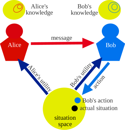
Figure 3: Sketch of the investigated communication scenario. Alice communicates parts of her knowledge to Bob about an unknown situation. After updating according to Alice’s message Bob chooses his action, which for simplicity is here assumed to be a point in situation space $\mathcal{S}$ (for example, the blue point could indicate to which situation his action is best adapted). His action and the unknown situation determine Bob’s resulting utility. Bob chooses his action by maximizing his expected utility given his knowledge after Alice informing him (blue equal probability contours of $\mathcal{P}(s|I_{\text{B}})$ in his mental copy of the situation space). The action and situation also determine a utility for Alice, which may or may not equal Bob’s utility. Alice chooses her message such that her expected utility resulting from Bob’s action is maximized in the light of her situation knowledge $\mathcal{P}(s|I_{\text{A}})$ (red contours). In case she is honest, she can only choose which parts of her knowledge she reveals with her message by deciding on a message topic $f(s)$; the message data is then determined to be $d=\langle f(s)\rangle_{(s|I_{\text{A}})}$.

In the following we investigate the scenario sketched in Fig. 3: Alice is relatively well informed about the situation $s\in\mathcal{S}$ her communication partner Bob will find himself in. In this not perfectly known situation Bob needs to take an action $a\in\mathbb{A}$, which is rewarded by a utility $u_{\text{B}}(s_{*},a)\in\mathbb{R}$ to Bob that depends on the situation $s_{*}\in\mathcal{S}$ that will eventually occur. Bob’s action also implies a utility $u_{\text{A}}(s_{*},a)\in\mathbb{R}$ to Alice. We will eventually assume that Alice’s and Bob’s utility functions are aligned, $u_{\text{A}}(s,a)=u_{\text{B}}(s,a)=:u(s,a)$, and give arguments why this might happen, but for the moment, we keep them separate in order to study the consequences of different interests.

Such misalignments are actually very common. Just imagine that Bob is Alice’s young child, $a$ is the amount of sugar that Bob is going to consume, and $s$ is how well his metabolism handles sugar. There is a lot of anecdotal evidence for $u_{\text{A}}(s,a)\neq u_{\text{B}}(s,a)$ under such conditions.

Alice will communicate through a bandwidth limited channel parts of her knowledge to Bob, who is here assumed to trust Alice fully, so that Bob can perform a more informed decision on his action. As stated before, Alice’s message takes the form $``\langle f(s)\rangle_{(s|I_{A})}=d"$, with $f:\mathcal{S}\rightarrow\mathbb{R}^{n}$, the conversation topic, being a moment function over the set of situations out of a limited set $\mathcal{F}$ of such functions she can choose from.

With increasing set size of $\mathcal{F}$ Alice’s communication channel becomes more flexible and with increasing dimension $n$ of the data space the channel bandwidth increases. Her message $m$ to Bob therefore consists of the tuple $(f,d)\in\mathcal{F}\times\mathbb{R}^{n}$.

In case

$$\langle f(s)\rangle_{(s|I_{A})}=d$$ (35)

actually holds as communicated, Alice is honest, otherwise she lies.

Alice assumes Bob to perform a knowledge update $I_{0}\overset{m}{\rightarrow}I_{\text{B}}$ following the MEP upon receiving her message $m=(f,d)$ such that

$$\langle f(s)\rangle_{(s|I_{\text{B}})} = d.$$ (36)

Thus, by choosing $f$ and $d$ Alice can directly determine certain expectation values of Bob’s knowledge, which then influence Bob’s action.

3.2 Optimal Action

The action Bob chooses optimally is

$$a_{\text{B}} = \underset{a\in\mathbb{A}}{\text{argmax}}\,u_{\text{B}}(a|I_{\text{B}})\text{, with}$$ (37)

$$u_{B}(a|I_{\text{B}}) = \langle u_{\text{B}}(s,a)\rangle_{(s|I_{\text{B}})}.$$ (38)

For simplicity we assume that this action is uniquely determined and that $u_{B}(a|I_{B})$ is twice differentiable w.r.t. $a$. Then, we find that $a_{\text{B}}$ solves

$$0 = \left.\frac{\partial u_{\text{B}}(a|I_{\text{B}})}{\partial a}\right|_{a=a_{\text{B}}}=\left\langle g_{\text{B}}(s,a_{\text{B}})\right\rangle_{(s|I_{\text{B}})}\!\!\text{,}$$ (39)

$$g_{\text{B}}(s,a) := \frac{\partial u_{\text{B}}(s,a)}{\partial a},$$ (40)

meaning that for the action $a_{\text{B}}$ Bob chooses, his expectation for his utility gradient $g_{\text{B}}(s,a)$ w.r.t. his action has to vanish.

From Alice’s perspective, Bob’s optimal action $a$ would be

$$a_{\text{A}} = \underset{a\in\mathbb{A}}{\text{argmax}}\,u_{\text{A}}(a|I_{\text{A}})\text{, with}$$ (41)

$$u_{\text{A}}(a|I_{\text{A}}) = \langle u_{\text{A}}(s,a)\rangle_{(s|I_{\text{A}})},$$ (42)

implying that $a_{\text{A}}$ solves

$$0 = \left.\frac{\partial u_{\text{A}}(a|I_{\text{A}})}{\partial a}\right|_{a=a_{\text{A}}}=\left\langle g_{\text{A}}(s,a_{\text{A}})\right\rangle_{(s|I_{\text{A}})}\!\!,$$ (43)

$$g_{\text{A}}(s,a) := \frac{\partial u_{\text{A}}(s,a)}{\partial a}.$$ (44)

3.3 Dishonest Communication

Let’s first investigate the scenario of Alice being so eager to manipulate Bob’s action to her advantage that she is willing to lie for that. In order that Bob does what Alice finds optimal for herself, $a_{\text{B}}=a_{\text{A}}$, she needs to manipulate Bob’s updated knowledge state $I_{\text{B}}$ such that

$$\left\langle g_{\text{B}}(s,a_{\text{A}})\right\rangle_{(s|I_{\text{B}})}=0,$$ (45)

according to Eq. 39. Thus, it would be advantageously for her if Bob’s expected utility gradient $g_{\text{B}}(s,a_{\text{A}})$ vanishes for the action $a_{\text{A}}$, which Alice prefers him to take, since then he would take this action, $a_{\text{B}}=a_{\text{A}}$. Alice can achieve this by setting his expectation for $g_{\text{B}}(s,a_{\text{A}})$ to zero via communicating him an appropriate deceptive message. Any message $m=(f,d)$ with the topic being $f(s)=g_{\text{B}}(s,a_{\text{A}})+c$ and the data $d=c$ will achieve that Eq. 45 is satisfied. Here $c\in\mathbb{R}^{n}$ is an arbitrary constant Alice might use to ensure $f\in\mathcal{F}$ (if this is possible) or to obscure her manipulation. As her deceptive communication derives from Alice’s knowledge and utility, these quantities imprint onto her message. This happens through the usage of her optimal action $a_{\text{A}}$ in $g_{\text{B}}(s,a)$ in Eq. 45. This by her preferred action is specified by Eq. 41.

Thus, Alice will use a communication topic $f$ that reflects Bob’s interest, as it is built on $g_{\text{B}}(\cdot,a)$, however evaluated for Alice’s preferred action $a_{\text{A}}$ in this scenario. In order for her manipulation to work, she has to make Bob believe that $\left\langle g_{\text{B}}(s,a_{\text{A}})\right\rangle_{(s|I_{\text{B}})}=0$ and hope that this will let him indeed choose $a=a_{\text{A}}$.

Interestingly, Alice does not need to know Bob’s initial knowledge state $I_{0}$ for this, as the MEP update ensures that the relevant moment of Bob’s updated knowledge $I_{\text{B}}$ gets the necessary value, see Eq. 45. Nevertheless, she needs to know his interests $g_{\text{B}}(s,a)$, as through exploiting those she can manipulate his action.

In the likely case of $d\neq\left\langle f(s)\right\rangle_{(s|I_{\text{A}})}$, Alice would be lying. However, lying is risky for Alice, since Bob might detect her lies in the long run, being it for Bob’s knowledge after Alice informing him $\mathcal{P}(s|I_{\text{B}})$ turns out too often to be a bad predictor for $s$, or by other telltale signs of Alice. Bob realizing that Alice lies could have negative consequences for her in the long run, therefore we assume in the following that Alice is always honest. However, she might still follow her own interests.

3.4 Topics under Misaligned Interests

What Alice faces in the general case of differing interests is a complex mathematical problem. Even if Alice is bound to be honest, she still has some influence on Bob by deciding which part of her knowledge she shares. She does not need to give him information that would drive his decision against her own interests. By choosing the conversation topic smartly, Alice could make Bob acting in a way that is beneficial to both of them to some degree.

Let us assume for now that Alice knows both utility functions, Bob’s and her own, as well as Bob’s initial knowledge $\mathcal{P}(s|I_{0})$. For a given $f\in\mathcal{F}$ used as the topic of her honest communication $m=(f,\langle f(s)\rangle_{(s|I_{\text{A}})})$, she can work out Bob’s resulting updated knowledge $I_{\text{B}}$=$I_{\text{B}}(f)$, his action $a$, as well as how advantageous that action would be for her, by calculating and optimizing

$$u_{\text{A}}(f) := \left\langle u_{\text{A}}(s,a_{\text{B}}(f))\right\rangle_{(s|I_{\text{A}})}\text{, with}$$ (46)

$$a_{\text{B}}(f) := \underset{a\in\mathbb{A}}{\text{argmax}}(u_{\text{B}}(a|I_{\text{B}}(f))),$$ (47)

$$u_{\text{B}}(a|I_{\text{B}}) := \left\langle u_{\text{B}}(s,a)\right\rangle_{(s|I_{\text{B}})},$$ (48)

$$\mathcal{P}(s|I_{\text{B}}(f)) = \frac{\mathcal{P}(s|I_{0})\,\exp\left(\mu\,f(s)\right)}{\mathcal{Z}(\mu,f)},$$ (49)

$$\mathcal{Z}(\mu,f) = \int\text{d}s\,\mathcal{P}(s|I_{0})\,\exp\left(\mu\,f(s)\right)\text{, with}$$ (50)

$$\mu=\mu(f):\,d \!\!\!\!\!\!\!\!\!\!\!\!=\!\!\!\!\!\!\!\!\!\!\!\! \frac{\partial\ln\mathcal{Z}(\mu,f)}{\partial\mu}.$$ (51)

The last step here, determining $\mathcal{P}(s|I_{\text{B}})$, is also an optimization problem according to the MEP. Thus, the optimal topic for Alice therefore results from the three fold nested optimization

$$f \!\!=\!\! \underset{f}{\text{argmax}\,}u_{\text{A}}(\underset{a}{\text{argmax}}\,u_{\text{B}}(a|f,\underset{I_{\text{B}}:\langle f(s)\rangle_{I_{\text{B}}}=\langle f(s)\rangle_{I_{\text{A}}}\!\!\!\!\!\!\!\!\!\!\!\!\!\!\!\!\!\!\!\!\!\!\!\!\!\!\!\!\!\!\!}{\text{argmax}}(\mathcal{D}_{s}(I_{\text{B}},I_{0}))).$$

Analytic solutions to this can only be expected in special cases. For future reference and numerical approaches to the problem, we calculate the relevant gradient $\partial u_{\text{A}}/\partial f$ in App. D. Its component for $s_{*}$ is

$$\frac{\text{d}u_{\text{A}}(f)}{\text{d}f(s_{*})}\!\!\!\! = \!\!\!\!-\left\langle g_{\text{A}}(s,a)\right\rangle_{(s|I_{\text{A}})}^{\text{t}}\left[\frac{\partial^{2}u_{\text{B}}(a|I_{\text{B}})}{\partial a\partial a^{\text{t}}}\right]^{-1}\times$$

$$\!\!\!\!\left\{g_{\text{B}}(s_{*},a)\,\mathcal{P}(s_{*}|I_{\text{B}})\,\mu^{\text{t}}-\left\langle g_{\text{B}}(s,a)\delta f(s)^{\text{t}}\right\rangle_{(s|I_{\text{B}})}\right.$$

$$\!\!\!\!\left.\times\left\langle\delta f(s)\,\delta f(s)^{\text{t}}\right\rangle_{(s|I_{\text{B}})}^{-1}\left[\mathcal{P}(s_{*}|I_{\text{B}})-\mathcal{P}(s_{*}|I_{\text{A}})\right]\right\},$$

where $a=a_{\text{B }}(f)$, $\mathcal{P}(s_{*}|I_{\text{B}})=\mathcal{P}(s_{*}|I_{\text{B}}(f))$, and $\mu=\mu(f)$ are given by Eq. 47, 49, and 51, respectively, and $\delta f(s):=f(s)-\left\langle f(s)\right\rangle_{(s|I_{\text{B}})}$. Inspection of the condition $\partial u_{\text{A}}/\partial f=0$ and the terms that could allow for it is instructive, as it hints to the factors that drive Alice’s topic choice. Alice has found a local optimal topic for her communication when either

• $g_{\text{A}}(a|I_{\text{A}}):=\left\langle g_{\text{A}}(s,a)\right\rangle_{(s|I_{\text{A}})}=0$, meaning that Alice’s remaining interest $g_{\text{A}}(a|I_{\text{A}})$ is perfectly satisfied by Bob’s resulting action $a$,

• for any situation $s_{*}$ a sophisticated balance $b(s_{*}):=\left\{\text{terms in curly brackets of Eq.\ \ref{eq:topic_gradient}}\right\}=0$ holds between Bob’s interest $g_{\text{B}}(s_{*},a)$ in that situation and the difference in the probabilities Alice and Bob assign to it, $\mathcal{P}(s_{*}|I_{\text{B}})-\mathcal{P}(s_{*}|I_{\text{A}})$, or

• the not balanced term $b(s_{*})$ is orthogonal to Alice’s remaining interest $g_{\text{A}}(a|I_{\text{A}})$ w.r.t. a metric given by the inverse Hessian of Bob’s expected utility $u_{\text{B}}(a|I_{\text{B}})$ (as derived w.r.t. his action $a$),

and the corresponding location is not a minimum of the expected utility.

Detailed investigation of the general case of misaligned interests are left for future work. Here, only an illustrative example will be examined.

3.5 Example of Misaligned Interests

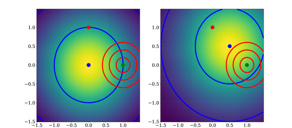
Figure 4: Knowledge states and preferred actions of Alice and Bob in case of misaligned interests before (left) and after (right) the communication. The plane of $s$-values is shown. Bob’s knowledge state initially, $\mathcal{P}(s|I_{0})$ (left), and finally, $\mathcal{P}(s|I_{\text{B}})$ (right), is shown by the background color as well as by the blue contour lines at the 1- and 2-sigma levels. Alice’s more precise knowledge is indicated only via red 1-, 2-, and 3-sigma level contours. The dots mark possible actions for Bob that are optimal for him under his knowledge (blue), under Alice’s knowledge (green), or optimal for Alice (red). Comparing the two panels, especially the movement of Bob’s optimal action (blue dot) between them, shows that Alice informs Bob such that he chooses an action that is a compromise between their interests.

An instructive example of misaligned interests is in order. For this, let us assume that the space of possible situations as well as that of actions have two dimensions, $s,a\in\mathbb{R}^{2}$. Alice’s and Bob’s initial beliefs shall be Gaussian distributions

$$\mathcal{P}(s|I^{\prime}_{\text{A/B}}) = \mathcal{G}(s-\overline{s}_{\text{A/B}},S_{\text{A/B}})\text{, with}$$ (54)

$$\mathcal{G}(s,S) := \frac{1}{||2\pi S||^{\nicefrac{{1}}{{2}}}}\exp\left(-\frac{1}{2}s^{\text{t}}S^{-1}s\right),$$ (55)

$\overline{s}_{\text{A}}=(1,0)^{\text{t}}$, $\overline{s}_{\text{B}}=(0,0)^{\text{t}}$, and $S_{\text{A}}<S_{\text{B}}=\mathbb{1}$ (spectrally), so that Alice is better informed than Bob (since $S_{\text{A}}<S_{\text{B}})$ and the chosen coordinate system is aligned with that knowledge ($s_{1}$-axis is parallel to $\overline{s}_{\text{A}}$). Furthermore, Bob’s utility should be

$$u_{\text{B}}(s,a)=-\left\|s-a\right\|^{2},$$ (56)

so that he wants his action to match the situation. Alice would prefer if he matched a by an angle $\varphi$ rotated target according to her utility

$$u_{\text{A}}(s,a) = -\left\|R\,s-a\right\|^{2}\text{, with}$$ (57)

$$R = \begin{pmatrix}\cos\varphi\,\,&-\sin\varphi\\ \sin\varphi\,&\cos\varphi\end{pmatrix}$$ (58)

establishing a misalignment of their interests.

In this situation, Bob’s expected utility is

$$u_{\text{B}}(a|I_{\text{B}})=-\left\langle s^{\text{t}}s\right\rangle_{(s|I_{\text{B}})}+2a^{\text{t}}\left\langle s\right\rangle_{(s|I_{\text{B}})}-a^{\text{t}}a,$$ (59)

from which his action

$$a_{\text{B}}=\left\langle s\right\rangle_{(s|I_{\text{B}})}$$ (60)

follows. Thus, the first moment of Bob’s belief on $s$ determines fully his action and therefore Alice only needs to inform him about that. Let us therefore assume that Alice will use a topic of the form $f(s)=\tau^{\text{t}}\,s$, with $\tau=(\cos\alpha,\sin\alpha)^{\text{t}}$ some normalized direction, so that $\tau^{\text{t}}\tau=1$. We check later using Eq. 3.4 whether this is her best choice or not.

The data of her message is then

$$d=\tau^{\text{t}}\left\langle s\right\rangle_{(s|I_{\text{A}})}=\tau^{\text{t}}\overline{s}_{\text{A}}=\cos\alpha$$ (61)

and Bob’s updated knowledge state becomes

$$\mathcal{P}(s|I_{\text{B}}) = \mathcal{G}(s-d\,\tau,\mathbb{1}),$$ (62)

as verified in the following: The MEP fixes Bob’s updated knowledge to be of the form

$$\mathcal{P}(s|I_{\text{B}}) = \frac{\exp\left(-\frac{1}{2}s^{\text{t}}s+\mu\,\tau^{\text{t}}s\right)}{\text{$2\pi$}\mathcal{Z}}\text{ with}$$ (63)

$$\mathcal{Z} = e^{\mu^{2}/2}.$$ (64)

Requiring that the communicated moment is matched leads to

$$\ln\mathcal{Z} = \frac{\mu^{2}\,}{2},$$ (65)

$$\frac{\partial\ln\mathcal{Z}}{\partial\mu} = \mu=d=\tau^{\text{t}}\overline{s}_{\text{A}}=\cos\alpha\text{, and}$$ (66)

$$\mathcal{P}(s|I_{\text{B}}) = \frac{\exp\left(-\frac{1}{2}\left[s^{\text{t}}s-2\,d\,\tau^{\text{t}}s+d^{2}\right]\right)}{\text{2$\pi$}}$$ (67)

$$= \mathcal{G}(s-d\,\tau,\mathbb{1}),$$

as we claimed. This implies $a_{\text{B}}=d\,\tau=\tau\,\tau^{\text{t}}\overline{s}_{\text{A}}$. Thus in this situation Bob does exactly what Alice tells him, as $a_{\text{B}}=d\,\tau$ consists of the two essential elements of her message $m=(\tau^{\text{t}}s,d)$. However, being honest, Alice is not fully free in what she can say. With choosing the topic direction $\tau$ the message’s data $d=\tau^{\text{t}}\overline{s}_{\text{A}}$ are fully determined thanks to her honesty.

Therefore, Alice’s expected utility

$$u_{\text{A}}(a) = -\left\langle s^{\text{t}}R^{\text{t}}Rs\right\rangle_{(s|I_{\text{A}})}+2d^{\text{t}}R\overline{s}_{\text{A}}-d^{\text{t}}d$$

$$= -\text{\text{t}r}\left\langle ss^{\text{t}}\right\rangle_{(s|I_{\text{A}})}+2\overline{s}_{\text{A}}^{\text{t}}\tau\,\tau^{\text{t}}\,R\overline{s}_{\text{A}}-\overline{s}_{\text{A}}^{\text{t}}\overline{s}_{\text{A}}$$

$$= -\text{\text{t}r}(S_{\text{A}}+\overline{s}_{\text{A}}\overline{s}_{\text{A}}^{\text{t}})-\overline{s}_{\text{A}}^{\text{t}}\overline{s}_{\text{A}}+2\overline{s}_{\text{A}}^{\text{t}}\tau\,\tau^{\text{t}}\,R\overline{s}_{\text{A}}$$

$$= -\text{\text{t}r}(S_{\text{A}})+2\cos\alpha\,\left(\cos\alpha\cos\varphi+\sin\alpha\sin\varphi\right)$$

becomes maximal for the topic direction

$$\alpha = \arctan\left[\frac{-\cos\varphi\pm 1}{\sin\varphi}\right],$$ (69)

as a straightforward calculation shows. The sign of $\pm$ has to be chosen such that $u_{\text{A}}(a)$ is maximal, which for $\varphi\in[-\pi,\pi]$ turns out to be $+$.

For mostly aligned interests, $\varphi\ll 1$, Alice’s optimal topic has an angle of $\alpha=\frac{1}{2}\varphi+\mathcal{O}(\varphi^{3})$, which means it is a nearly perfect compromise between what is optimal for her and for Bob. For $\alpha=0$ their interests are perfectly aligned and Alice informs Bob ideally with the statement “$\langle s_{1}\rangle_{(s|I_{\text{A}})}=1$”.

In case of orthogonal interests, $\varphi=\pi/2$, Alice’s optimal topic angle is $\alpha=\pi/4$, informing effectively with a statement like “$\langle s_{1}+s_{2}\rangle_{(s|I_{\text{A}})}=1$”, which, given that $\langle s\rangle_{(s|I_{\text{A}})}=(1,0)^{\text{t}}$, is less informative for Bob than the statement “$\langle s_{1}\rangle_{(s|I_{\text{A}})}=1$” Alice would have made under aligned interests. Bob’s resulting decision of $a=(\nicefrac{{1}}{{2}},\nicefrac{{1}}{{2}})^{\text{t}}$ in that case turns out to be a perfect compromise between their interests, or put differently being sub-optimal for each of them to the same degree. This situation is depicted in Fig. 4.

For anti-aligned interests, $\varphi=\pi$, Alice’s optimal topic angle is $\alpha=\pi/2$ as then she can only send the uninformative message “$\langle s_{2}\rangle_{(s|I_{\text{A}})}=0$”, as revealing any more of her knowledge would be against her interests. This leaves Bob’s knowledge unchanged and therefore lets him pick the action $a=\overline{s}_{\text{B}}=(0,0)^{\text{t}}$.

To summarize, misalignment of interests leads to a communication and a resulting action that are a compromise between the interests of the communication partners. Who of the two has to compromise more depends on details of their knowledge states and their interests.

Alice informing Bob sub-optimally to her own advantage bears for Alice the risk of Bob realizing this. In repeated situations, Bob might recognize the systematic misalignment angle $\alpha=\text{angle}(s,a)$ between the $s_{*}$ that happened and the topic direction $\tau$ chosen by Alice on the basis of her information on $s$. This might either let him question Alice’s good intentions for him or her competence. In either case he could threaten Alice to ignore or even counteract against her advice until he gets convinced that she has largely aligned her interests with his.

The general optimal topic of Alice’s message could, however, be a non-linear function of the situation instead of the linear $f(s)=\tau^{\text{t}}s$ assumed above. This can be checked by inspecting the functional gradient of $u_{\text{A}}(f)$ w.r.t. $f$ as given by Eq. 3.4. In case it vanishes for all $s\in\mathcal{S}$ the topic was optimal.

It turns out that this gradient only vanishes when Alice’s and Bob’s interests are aligned ($\varphi=0$), as shown in App. E. For the instructive case of orthogonal interests ($\varphi=\nicefrac{{\pi}}{{2}}$), however, the gradient

$$\frac{\text{d}u_{\text{A}}(f)}{\text{d}f(s)}\!\!\!\! = \!\!\!\!\frac{s_{2}-s_{1}}{\sqrt{2}}\,\mathcal{P}(s|I_{\text{B}})$$ (70)

does not vanish. This indicates that she could construct a more sophisticated message that would pull Bob’s resulting action a bit closer towards her own interest $a_{\text{A}}$ and further away from the action optimal for him (under her knowledge). The precise form of the optimal topic for Alice is left for future work.

3.6 Aligned Interests

In the following we assume that Alice simply wants the best for Bob from his perspective ($a_{\text{A}}=a_{\text{B}}$) and therefore adapts his utility for herself,

$$u_{\text{A}}(s,a)=u_{\text{B}}(s,a)=:u(s,a).$$

In this case, Alice informs Bob optimally via the message $m=(f,d)$ with $f(s)=g_{\text{A}}(s,a_{\text{A}})+c=g_{\text{B}}(s,a_{\text{B}})+c$, which leads to a synchronization of their expectations w.r.t. the most relevant moment of $s,$ $\langle f(s)\rangle_{(s|I_{\text{A}})}=\langle f(s)\rangle_{(s|I_{\text{B}})}$, and therefore to an alignment of their optimal actions, $a_{\text{A}}=a_{\text{B}}=:a_{*}$.

For simplicity, we assume in the following that the action is described by one real number $a\in\mathbb{R}$. An extension to a vector valued action space $\mathcal{A}=\mathbb{R}^{u}$ is straightforward, but does not add too much to the discussion below except of complexity in the notation. Furthermore we assume Alice and Bob’s common utility function to be uni-modal in a given situation and to be well approximated within the relevant region by

$$u(s,a)=v(s)-\frac{1}{2k}\left(\frac{a-b(s)}{\sigma(s)}\right)^{2k}.$$ (71)

Here, $b(s)$ is the optimal action in a given situation $s$, $v(s)$ the utility of this optimal action, $\sigma(s)\in\mathbb{R^{+}}$ the tolerance for deviation from the optimal action, and $k\in\mathbb{N}$ is specifying how harsh larger deviations reduce the utility. This should serve as a sufficiently generic model that can capture a large variety of realistic situations. In particular the case of a quadratic loss (=negative utility) with $k=1$ mimics the typical situation in which a Taylor expansion in $a$ around the optimal action $b(s)$ can be truncated after the quadratic term.

Alice’s expected utility of Bob’s action

$$u(a|I_{\text{A}})=\langle u(s,a)\rangle_{(s|I_{\text{A}})}$$ (72)

has the gradient

$$\frac{\partial u(a|I_{\text{A}})}{\partial a} = -\left\langle\frac{\left[a-b(s)\right]^{2k-1}}{\left[\sigma(s)\right]^{2k}}\right\rangle_{(s|I_{\text{A}})}$$ (73)

$$= -\sum_{n=0}^{2k-1}b_{n}a^{n},\text{with}$$ (74)

$$b_{n} = \begin{pmatrix}2k-1\\ n\end{pmatrix}\left\langle\frac{\left[-b(s)\right]^{2k-1}}{\left[\sigma(s)\right]^{2k}}\right\rangle_{(s|I_{\text{A}})}.$$ (75)

This is a polynomial of odd order in $a$ and therefore guaranteed to have at least one real root. The maximum of $u(a|I_{\text{A}})$ among all such roots then gives the optimal action $a_{*}$. Thus, the topic function

$$f(s)=\frac{\left[a_{*}-b(s)\right]^{2k-1}}{\left[\sigma(s)\right]^{2k}}+c$$

is Alice’s best choice for a communication that ensures that Bob makes an optimal decision.

In case $b(s)=s$ and $\sigma(s)=1$ this is $f(s)=(a_{*}-s)^{2k-1}$, which is a polynomial of order $2k-1$ in $s$. Instead of communicating the expectation value of this polynomial, which requires her to work out $a_{*}$, Alice could simply communicate all moments up to order $2k-1$ and thereby ensure that Bob would have all information needed in order to decide on the optimal action.

Here, the requirement of properness appears in a weak form. Alice wanting to inform Bob on a number of moments of her knowledge in order to put him into a position to make a good decision is a weak form of the requirement of properness. Full properness would be that Alice wants to inform Bob to know all possible moments of her knowledge. Thus, properness is expected to occur when Alice does not know Bob’s utility function, but wants to support him no matter what his interests are. We will now turn to such a scenario.

4 Attention

We saw why Alice might align her interest with Bob’s and in the following assume this to have happened, $u_{\text{A}}=u_{\text{B}}\equiv u$. Her knowledge on Bob’s utility function influences how she selects her message optimally. For the concept of attention to appear in her reasoning, Alice must not know Bob’s utility function in detail. In case she did, she would optimize for the utility function. However, she needs to be aware of the sensitivity with which Bob’s utility reacts to Bob’s choices in the different situations $s$ in order to give those situations appropriate weights in her communication. These weights will determine how accurately she should inform about the different situations such that Bob is optimally prepared to make the right decision.

To be concrete, let Alice assume that in a given situation $s$ Bob’s utility has a single maximum at some to her unknown optimal action $a_{*}(s)=b(s)$ of a to her unknown height $u(s,a_{*}(s))=v(s)$, but with a to her known curvature $w(s)$. Furthermore, she assumes that this utility function can be well Taylor-approximated around any of these maxima as

$$u(s,a,v,w,b)=v(s)-\frac{1}{2}w(s)\left(a-b(s)\right)^{2}.$$ (76)

This corresponds to the case of Eq. 71 with $k=1$ and $\sigma(s)=\left[w(s)\right]^{-1/2}$. We have added the parameters $v$, $w$, and $b$ to the list of arguments of this approximate utility function as Alice needs to average over the ones unknown to her, which are $v$ and $b$.

In order to circumvent the technical difficulty to deal with probabilities over functional space let us restrict the following discussion to discrete $s\in\mathcal{S}.$ In this case the parameters $v$, $w$, and $b$ become finite dimensional vectors with components $v_{s}=v(s)$, etc.. The case of a continuous set of situations is dealt with in App. F.

Alice assumes that Bob’s action will depend on these parameters and is given by

$$a_{*}(v,b,\sigma,I_{B}) = \text{argmax}_{a}\left\langle u(s,a,v,w,b)\right\rangle_{(s|I_{\text{B}})}$$ (77)

$$= a:\left[\left\langle\frac{\partial u(s,a,v,w,b)}{\partial a}\right\rangle_{(s|I_{\text{B}})}=0\right]$$

$$= a:\left[-\left\langle\left[a-b(s)\right]\,w(s)\right\rangle_{(s|I_{\text{B}})}=0\right]$$

$$= \frac{\left\langle b(s)\,w(s)\right\rangle_{(s|I_{\text{B}})}}{\left\langle w(s)\right\rangle_{(s|I_{\text{B}})}}$$

$$=: \left\langle b(s)\right\rangle_{(s|I_{\text{B}})}^{(w)},$$

where $a:\left[f(a)=0\right]$ means the (here assumed to be unique) value of $a$ that fulfills $f(a)=0$. Furthermore, we introduced the $w$-weighted expectation value

$$\left\langle b(s)\right\rangle_{(s|I_{\text{B}})}^{(w)}:=\sum_{s\in\mathcal{S}}\,b(s)\,\mathcal{A}^{(w)}(s|I_{\text{B}})$$ (78)

that involves the attention $\mathcal{A}^{(w)}(s|I_{\text{B}})$ defined in Eq. 3.

Let us assume that Alice believes that the curvature of Bob’s utility maxima are $w_{*}(s)$. This might be because she can estimate the influence Bob’s actions have on his own well being in the different situations. For example, in the extreme case that Bob might be dead in a given $s_{*}$, she might set $w_{*}(s_{*})=0$ as none of the possible actions of Bob then matter any more to him. It will turn out that the actual values of $w(s)$ do not matter, only their relative values w.r.t. each other.

Thus, her knowledge about Bob’s utility is

$$\mathcal{P}(v,b,w|I_{\text{A}})=\delta(w-w_{*})\,\mathcal{P}(v,b|I_{\text{A}}),$$ (79)

with $\mathcal{P}(v,b|I_{\text{A}})$ a relatively uninformative probability density. We assume this to be independent on her knowledge on the situation, $\mathcal{P}(s,v,b|I_{\text{A}})=\mathcal{P}(s|I_{\text{A}})\mathcal{\,P}(v,b|I_{\text{A}})$.

Furthermore, we assume here, in order to have a simple instructive scenario, that Alice only has a vague idea around which value $\overline{b}:=\langle b(s)\rangle_{(b,s|I_{\text{A}})}$ the location of the maximum $b(s)$ of Bob’s utility could be, and how much it could deviate from $\overline{b}$. We assume that she is not aware of any correlation of this function nor any structure of its variance and therefore define

$$\overline{b}(s) := \left\langle b(s)\right\rangle_{\!(b|I_{\text{A}})}=\overline{b},$$ (80)

$$D(s,s^{\prime}) := \left\langle\left(b(s)-\overline{b}(s)\right)\,\left(b(s^{\prime})-\overline{b}(s)\right)\right\rangle_{\!(b|I_{\text{A}})}$$ (81)

$$=: \gamma^{2}\,\delta_{s\,s^{\prime}}.$$ (82)

In the last step we used that Alice’s knowledge on $b$ is uninformative, therefore unstructured, and thus its uncertainty covariance proportional to the unit matrix. The parameter $\gamma$ expresses how much variance Alice expects in $b$. Its precise value will turn out to be irrelevant.

Other setups in which $\overline{b}(s)$ is not a constant or $D(s,s^{\prime})$ contain cross-correlations, are addressed in App. F.

With the above assumptions, the expected utility is

$$u(I_{\text{B}}) = \left\langle u\left(s,a_{*}(v,w,b),v,w,b\right)\right\rangle_{\!(s,v,w,b|I_{\text{A}})}$$

$$= \left\langle u\left(s,\left\langle b(s)\right\rangle_{(s|w,I_{\text{B}})},v,w,b\right)\right\rangle_{\!(s,v,b,\sigma|I_{\text{A}})}$$

$$= \left\langle v(s)-\frac{w(s)}{2}\left(\left\langle b(s)\right\rangle_{(s|w,I_{\text{B}})}-\overline{b}\right)^{2}\right\rangle_{\!\!(s,v,w,b|I_{\text{A}})}$$

$$= \underbrace{\left\langle v(s)\right\rangle_{(s,v|I_{\text{A}})}}_{=:V(I_{\text{A}})}-\frac{1}{2}\underbrace{\left\langle w_{*}(s)\right\rangle_{(s|I_{\text{A}})}}_{=:w_{I_{\text{A}}}}\times$$

$$\left\langle\left(\left\langle b(s)\right\rangle_{(s|w_{*},I_{\text{B}})}-\overline{b}\right)^{2}\right\rangle_{(s,b|I_{\text{A}})}^{(w_{*})}$$

$$= V(I_{\text{A}})-\frac{w_{I_{\text{A}}}}{2}\times\left\langle\left(\left\langle b(s)\right\rangle_{(s|I_{\text{B}})}^{(w_{*})}\right)^{2}\right.$$

$$-2\left\langle b(s)\right\rangle_{(s|I_{\text{B}})}^{(w_{*})}\left\langle b(s)\right\rangle_{(s|I_{\text{A}})}^{(w_{*})}$$

$$\left.+\left\langle b^{2}(s)\right\rangle_{(s|I_{\text{A}})}^{(w_{*})}\right\rangle_{(b|I_{\text{A}})}$$

$$=: V(I_{\text{A}})-\frac{w_{I_{\text{A}}}}{2}\left(\text{I}-2\text{II}+\text{III}\right).$$ (85)

The three terms I-III occurring therein are

​​​​​​​​I $$:= \left\langle\left(\left\langle b(s)\right\rangle_{(s|I_{\text{B}})}^{(w_{*})}\right)^{2}\right\rangle_{(b|I_{\text{A}})}$$ (86)

$$= \sum_{s,s^{\prime}\in\mathcal{S}}\mathcal{A}(s|I_{\text{B}})\,\mathcal{A}(s^{\prime}|I_{\text{B}})\,\left\langle b(s)\,b(s^{\prime})\right\rangle_{(b|I_{\text{A}})}\!\!\!\!\!\!\!\!\!\!\!\!\!\!\!\!$$

$$= \sum_{s,s^{\prime}\in\mathcal{S}}\mathcal{A}(s|I_{\text{B}})\,\mathcal{A}(s^{\prime}|I_{\text{B}})\,\left(\overline{b}^{2}+\gamma^{2}\delta_{s\,s^{\prime}}\right)\!\!\!\!\!\!\!\!\!\!\!\!\!\!\!\!$$

$$= \overline{b}^{2}+\gamma^{2}\sum_{s\in\mathcal{S}}\,\left[\mathcal{A}(s|I_{\text{B}})\right]^{2}$$

II $$:= \left\langle\left\langle b(s)\right\rangle_{(s|I_{\text{B}})}^{(w_{*})}\left\langle b(s)\right\rangle_{(s|I_{\text{A}})}^{(w_{*})}\right\rangle_{(b|I_{\text{A}})}$$ (87)

$$= \sum_{s,s^{\prime}\in\mathcal{S}}\mathcal{A}(s|I_{\text{B}})\,\mathcal{A}(s^{\prime}|I_{\text{A}})\,\left(\overline{b}^{2}+\gamma^{2}\delta_{s\,s^{\prime}}\right)$$

$$= \overline{b}^{2}+\gamma^{2}\sum_{s\in\mathcal{S}}\,\mathcal{A}(s|I_{\text{A}})\,\mathcal{A}(s|I_{\text{B}})$$

III $$:= \left\langle\left\langle b^{2}(s)\right\rangle_{(s|I_{\text{B}})}^{(w_{*})}\right\rangle_{(b|I_{\text{A}})}$$ (88)

$$= \sum_{s\in\mathcal{S}}\,\mathcal{A}(s|I_{\text{B}})\left(\overline{b}^{2}+\gamma^{2}\right)$$

$$= \overline{b}^{2}+\gamma^{2},$$

where we wrote just $\mathcal{A}$ for $\mathcal{A}^{(w_{*})}$ for brevity. Inserting I-III into Eq. 4 gives

$$u(I_{\text{B}}) = V(I_{\text{A}})-\frac{w_{I_{\text{A}}}}{2}\gamma^{2}\times$$

$$\left\{\sum_{s\in\mathcal{S}}\,\left[\mathcal{A}(s|I_{\text{B}})\right]^{2}-2\sum_{s\in\mathcal{S}}\,\mathcal{A}(s|I_{\text{B}})\,\mathcal{A}(s|I_{\text{A}})+1\right\}$$

$$= -\frac{w_{I_{\text{A}}}}{2}\gamma^{2}\sum_{s\in\mathcal{S}}\,\left[\mathcal{A}(s|I_{\text{B}})-\mathcal{A}(s|I_{\text{A}})\right]^{2}+\text{const}(I_{\text{A}})$$

This expected utility needs to be maximized w.r.t. $I_{\text{B}},$ Bob’s knowledge after the update. It is obvious that the maximum is at $I_{\text{B}}=I_{\text{A}}$ as then $\mathcal{A}(s|I_{\text{B}})=\mathcal{A}(s|I_{\text{A}})$ and the negative term becomes zero.

At this maximum we have $\mathcal{P}(s|I_{\text{B}})=\mathcal{P}(s|I_{\text{A}})$ if $w_{*}(s)>0$ for all $s\in\mathcal{S}$, which means that Alice strives for communicating properly, if possible. Otherwise she tries to minimizes the $\mathcal{L}^{2}$-norm between her and Bob’s attention distribution functions.

In case $\mathcal{S}$ is continuous, properness appears as well as Alice’s optimal strategy if $G(s,s^{\prime}):=\overline{b}(s)\overline{b}(s^{\prime})+D(s,s^{\prime})$ is either diagonal, $G(s,s^{\prime})=\sigma_{b}^{2}(s)\,\delta(s-s^{\prime})$, or translation invariant, $G(s,s^{\prime})=G(s-s^{\prime})$, as is shown in App. F. If these conditions are not met, Alice will optimally transmit a biased attention to Bob.

5 Relative Attention Entropy

5.1 Derivation

We have seen how attention appears naturally in a communication scenario in which an honest sender tries to be supportive to the receiver, without knowing details of the receiver’s utility function except for having a guess for the variation of its narrowness in different situations. The measure used by such a sender to match the receiver’s attention function to the own one is then typically of a square distance form, like in Eq. LABEL:eq:utility-w-marginalized-2, maybe with some bias term as in Eq. 159. In any way, attention seems to be a central element of utility aware communication.

This poses the question whether there is a scenario in which relative attention entropy appears as the measure the sender should use to choose among possible messages. The answer to this question is yes.

In case Alice assumes that Bob will judge her prediction on the basis of how much attention was given to the situation that ultimately happened, and knows the weights Bob will apply to turn probabilities into attentions, as well as wants to be proper, if possible, the relative attention entropy can be derived analogously to the derivation of relative entropy in Sec. 2.1, as we see in the following.

Again, we require the measure to be analytical, proper, and calibrated, and only modify the requirement of locality to attention locality: Only Bob’s attention $\mathcal{A}(s_{*}|I_{\text{B}})$ for the case $s=s_{*}$ that happens in the end matters for Alice’s loss.

Again, at the time Alice has to make her choice, she does not know which situation $s=s_{*}$ will happen in the end, and therefore needs to minimize her expected loss

$$\mathcal{L}^{(w)}(I_{\text{A}},I_{\text{B}}) := \left\langle\mathcal{L}^{(w)}(s_{*},I_{\text{A}},I_{\text{B}})\right\rangle_{(s_{*}|I_{\text{A}})}$$ (90)

for deciding which knowledge state Bob $I_{\text{B}}$ should get (via her message $m$). This loss will depend on the weight function $w(s)$ that turns probabilities into attentions according to Eq. 3. We assume $w(s)>0$ for all $s\in\mathcal{S}$ in the following, such that $\mathcal{A}(s|I_{\text{A}})=\mathcal{A}(s|I_{\text{B}})$ for all $s\in\mathcal{S}$ implies $\mathcal{P}(s|I_{\text{A}})=\mathcal{P}(s|I_{\text{B}})$ for all $s\in\mathcal{S}$ and vice versa.

Attention locality implies that $\mathcal{L}^{(w)}(s,I_{\text{A}},I_{\text{B}})$ must depend on $I_{\text{B}}$ through $q(s):=\mathcal{A}(s|I_{\text{B}})$, whereas the dependence on $I_{\text{A}}$ could still be through $\mathcal{P}(s|I_{\text{A}})$. However, as the information content of $\mathcal{P}(s|I_{\text{A}})$ and $\mathcal{A}(s|I_{\text{A}})$ are equivalent, it is convenient to express the dependence on $I_{\text{A}}$ through $p(s):=\mathcal{A}(s|I_{\text{A}})$, as then properness is given when $q=p$.

Thus we have

$$\mathcal{L}^{(w)}(s,I_{\text{A}},I_{\text{B}})=\mathcal{L}^{(w)}(s,p(s),q(s))+\lambda\,\left(1-\int\text{d}s^{\prime}\,q(s^{\prime})\right),$$ (91)

where as before we use the function signatures to discriminate different $\mathcal{L}^{(w)}$’s and introduce a Lagrange multiplier to ensure that $q(s)$ is normalized.

Properness then requests that the expected loss should be minimal for $q=p$, implying for all possible $s=s_{*}$

$$0\!\!\!\!\! =\!\!\!\!\! \left.\frac{\partial\mathcal{L}^{(w)}(I_{\text{A}},I_{\text{B}})}{\partial q(s_{*})}\right|_{q=p}$$ (92)

$$=\!\!\!\!\! \left.\left\langle\frac{\partial}{\partial q(s_{*})}\left[\mathcal{L}^{(w)}(s,p(s),q(s))\!\text{\textasciiacute}-\!\lambda\!\!\int\text{d}s^{\prime}\,q(s^{\prime})\right]\right\rangle_{(s|I_{\text{A}})}\right|_{q=p}$$

$$=\!\!\!\!\! \left.\int\text{d}s\,\delta(s-s_{*})\left[\frac{\partial\mathcal{L}^{(w)}(s,p(s),y)}{\partial y}\right]_{y=q(s)}\!\!\!\!\mathcal{P}(s|I_{\text{A}})\right|_{q=p}\!\!\!\!-\lambda$$

$$=\!\!\!\!\! \left.\left[\frac{\partial\mathcal{L}^{(w)}(s,p(s_{*}),y)}{\partial y}\right]_{y=q(s_{*})}\!\!\!\!\frac{\frac{p(s_{*})}{w(s_{*})}}{\int_{\mathcal{S}}ds^{\prime}\,\frac{p(s^{\prime})}{w(s^{\prime})}}\right|_{q=p}\!\!\!\!-\lambda.$$

$$=\!\!\!\!\! \left.\left[\frac{\partial\mathcal{L}^{(w)}(s,x,y)}{\partial y}\right]_{y=x}\frac{x}{w(s_{*})\,\int_{\mathcal{S}}ds^{\prime}\,\frac{p(s^{\prime})}{w(s^{\prime})}}-\lambda\right|_{x=p(s_{*})}\!\!\!\!\!\!\!\!\!\!\!\!\!\!\!\!\!\!.$$

From this follows

$$\left[\frac{\partial\mathcal{L}^{(w)}(s,x,y)}{\partial y}\right]_{y=x}=\frac{\lambda\,w(s_{*})\,\int_{\mathcal{S}}ds^{\prime}\,\frac{p(s^{\prime})}{w(s^{\prime})}}{x},$$ (93)

which is solved analytically by

$$\mathcal{L}^{(w)}(s,x,y)=\lambda\,w(s)\,\int_{\mathcal{S}}ds^{\prime}\,\frac{p(s^{\prime})}{w(s^{\prime})}\,\ln\,y+c^{(w)}(s,x),$$ (94)

as can be verified by insertion. We note that

$$\int_{\mathcal{S}}ds\,\frac{p(s)}{w(s)} = \int_{\mathcal{S}}ds\,\frac{w(s)\,\mathcal{P}(s|I_{\text{A}})}{w(s)\int_{\mathcal{S}}ds^{\prime}w(s^{\prime})\,\mathcal{P}(s^{\prime}|I_{\text{A}})}$$ (95)

$$= \int_{\mathcal{S}}ds\,\frac{\mathcal{P}(s|I_{\text{A}})}{\int_{\mathcal{S}}ds^{\prime}w(s^{\prime})\,\mathcal{P}(s^{\prime}|I_{\text{A}})}$$

$$= \frac{1}{\int_{\mathcal{S}}ds^{\prime}w(s^{\prime})\,\mathcal{P}(s^{\prime}|I_{\text{A}})}$$

and choose $\lambda=1.$

Calibration requests then that $0=\mathcal{L}^{(w)}(s,x,x)$ and therefore

$$c(s,x)=-\frac{\lambda\,w(s)}{\int_{\mathcal{S}}ds^{\prime}w(s^{\prime})\,\mathcal{P}(s^{\prime}|I_{\text{A}})}\,\ln\,x$$ (96)

.

Thus, Alice’s loss function to choose the message

$$\mathcal{L}^{(w)}(I_{\text{A}},I_{\text{B}}) = \int_{\mathcal{S}}ds\,\mathcal{P}(s|I_{\text{A}})\times$$ (97)

$$\left[\frac{w(s)\,\left[\ln\,\mathcal{A}(s|I_{\text{A}})-\ln\,\mathcal{A}(s|I_{\text{B}})\right]}{\int_{\mathcal{S}}ds^{\prime}w(s^{\prime})\,\mathcal{P}(s^{\prime}|I_{\text{A}})}\right]$$

$$= \int_{\mathcal{S}}ds\,\mathcal{A}(s|I_{\text{A}})\,\ln\frac{\mathcal{A}(s|I_{\text{A}})}{\mathcal{A}(s|I_{\text{B}})}$$

$$= \mathcal{D}_{s}^{(w)}(I_{\text{A}},I_{\text{B}})$$

turns out to be the relative attention entropy. This closes its derivation.

5.2 Comparison to Other Scoring Rules

A brief comparison of relative attention entropy to other attention based score functions is in order.

First we note that in case the weights are constant, $w(s)=\text{const}$, relative attention entropy reduces to relative entropy.

For the comparison to the communication scenario of Sec. 4, in which Alice wants to support Bob as much as possible, but does only know the curvature of Bob’s utility, we investigated the limit of small relative difference between the attention function, $\Delta(s):=(\mathcal{A}(s|I_{\text{B}})-\mathcal{A}(s|I_{\text{A}}))/\mathcal{A}(s|I_{\text{A}})\ll 1$ for all $s\in\mathcal{S}$. In this case, relative attention entropy is well approximated by

$$\mathcal{D}_{s}^{(w)}(I_{\text{A}},I_{\text{B}}) \!\!\!\!=\!\!\!\! -\int_{\mathcal{S}}ds\,\mathcal{A}(s|I_{\text{A}})\,\ln\left[\frac{\mathcal{A}(s|I_{\text{B}})}{\mathcal{A}(s|I_{\text{A}})}\right]$$ (98)

$$\!\!\!\!=\!\!\!\! -\int_{\mathcal{S}}ds\,\mathcal{A}(s|I_{\text{A}})\,\ln\left[1+\left(\frac{\mathcal{A}(s|I_{\text{B}})}{\mathcal{A}(s|I_{\text{A}})}-1\right)\right]$$

$$\!\!\!\!=\!\!\!\! -\int_{\mathcal{S}}ds\,\mathcal{A}(s|I_{\text{A}})\,\left[\Delta(s)-\frac{1}{2}\Delta^{2}(s)+\ldots\right]$$

$$\!\!\!\!\approx\!\!\!\! \int_{\mathcal{S}}ds\,\left[\mathcal{A}(s|I_{\text{A}})-\mathcal{A}(s|I_{\text{B}})+\right.$$

$$\left.\frac{1}{2}\frac{(\mathcal{A}(s|I_{\text{B}})-\mathcal{A}(s|I_{\text{A}}))^{2}}{\mathcal{A}(s|I_{\text{A}})}\right]$$

$$\!\!\!\!=\!\!\!\! \frac{1}{2}\int_{\mathcal{S}}ds\,\frac{(\mathcal{A}(s|I_{\text{B}})-\mathcal{A}(s|I_{\text{A}}))^{2}}{\mathcal{A}(s|I_{\text{A}})},$$

which is the well-known information metric. Comparing this to the negative loss function of Eq. LABEL:eq:utility-w-marginalized-2, as generalized to the continuum by Eq. 159 gives under the assumptions of homogeneity and independence ($G(s,s^{\prime})\propto\delta(s-s^{\prime})$, see App. F for details)

$$-u(I_{\text{B}})\propto\frac{1}{2}\int_{\mathcal{S}}ds\,(\mathcal{A}(s|I_{\text{B}})-\mathcal{A}(s|I_{\text{A}}))^{2}+\text{const}(I_{\text{A}}).$$ (99)

There is at least one similarity between these scores, in that deviations between the attention functions should be avoided as the loss increases with their square. However, these scores also differ in a significant point, as for the attention entropy the deviation in attention functions is reversely weighted with Alice attention. This means that relative attention entropy allows for larger deviations in regions of higher attention compared to the utility based score, and smaller deviations in regions of low attention.

Finally, we note that weighted relative entropy as well as relative attention entropy are equivalent to scoring rules [25, 26]. Scoring rules evaluate how well a belief $I_{\text{B}}$ matches a probability $\mathcal{P}(s|I_{\text{A}})$ and are – in our notation – of the functional form

$$S(I_{\text{A}},I_{\text{B}})=\int_{S}ds\,\mathcal{P}(s|I_{\text{A}})\,\mathcal{L}(s,I_{\text{B}}),$$ (100)

with $\mathcal{L}$ being some loss function that expresses how bad it is to only believe with the strength $\mathcal{P}(s|I_{\text{B}})$ into an event $s\in\mathcal{S}$ that might happen, with the correct probability $\mathcal{P}(s|I_{\text{A}})$. Scoring rules are used to choose the “best fitting” belief among a set of beliefs, by picking the one that has the lowest score. They are called proper, if the best fit for $I_{\text{B}}$ is $I_{\text{A}}$ whenever the latter is part of the set of beliefs to choose $I_{\text{B}}$ from. Any additive, only $I_{\text{B}}$-independent affine transformations does not change the minimum of the score. Therefore those lead to identical results for $I_{\text{B}}$. Thus, we need only to show for our claim of equivalence that $\widetilde{\mathcal{D}}_{s}^{(w)}(I_{\text{A}},I_{\text{B}})$ and $\mathcal{D}_{s}^{(w)}(I_{\text{A}},I_{\text{B}})$ can be brought into the extended form

$$S^{\prime}(I_{\text{A}},I_{\text{B}})=a(I_{\text{A}})\int_{S}ds\,\mathcal{P}(s|I_{\text{A}})\,\mathcal{L}(s,I_{\text{B}})+b(I_{\text{A}}).$$ (101)

This works for weighted relative entropy by choosing

$$\mathcal{L}(s,I_{\text{B}}) = -w(s)\,\ln\mathcal{P}(s|I_{\text{B}})\text{,}$$ (102)

$$a(I_{\text{A}}) = 1\text{, and}$$ (103)

$$b(I_{\text{A}}) = \int_{\mathcal{S}}ds\,\mathcal{P}(s|I_{\text{A}})\,w(s)\,\ln\mathcal{P}(s|I_{\text{A}}),$$ (104)

as well as for relative attention entropy with

$$\mathcal{L}(s,I_{\text{B}}) = -w(s)\,\ln\mathcal{A}^{(w)}(s|I_{\text{B}})\text{,}$$ (105)

$$a(I_{\text{A}}) = \left[\int_{\mathcal{S}}\!ds\,w(s)\,\mathcal{P}(s|I_{\text{A}})\right]^{-1}\text{, and}$$ (106)

$$c(I_{\text{A}}) = \int_{\mathcal{S}}ds\,\mathcal{A}^{(w)}(s|I_{\text{A}})\,\ln\mathcal{A}^{(w)}(s|I_{\text{A}}).$$ (107)

Thus, the well developed formalism of scoring rules [26] can be used to investigate these entropies. It might be interesting to note in that context that weighted entropy is equivalent to a local scoring rule, since its $\mathcal{L}(s,I_{B})$ depends only on $\mathcal{P}(s|I_{\text{B}})$ for the $s$ in the argument of $\mathcal{L}$. However, attention entropy is (equivalent to)equivalent to a non-local score, as the normalization of the attention function in its $\mathcal{L}$ combines values of $\mathcal{P}(s|I_{\text{B}})$ for different $s$.

6 Conclusion

6.1 Properness, Attention, and Entropy

Entropy is a central element of communication theory. Relative entropy allows a sender to decide which message to send in order to inform about an unknown situation in case only the communicated probability of the situation that finally happens matters. Naively introducing an importance weighting for the different situations into relative entropy renders weighted relative entropy to be improper, meaning that it does not favor to transmit the sender’s precise knowledge state in case this is possible.

In order to find guidance how a weighting could be introduced into entropic communication properly, we investigated the scenario in which a sender, Alice, informs a receiver, Bob, about a situation that will matter for a decision on an action Bob will perform. The goal of this exercise is to find a scenario that encourages Alice to be on the one hand proper, and on the other hand to include weights into her considerations. Alice can decide which aspects of her knowledge she communicates and which she omits. In case the utility functions of Alice and Bob differ, Alice might be tempted to lie to Bob. This would certainly be improper. We argued that lying should be strongly discouraged if Alice and Bob interact repeatedly, as otherwise Bob might discover that Alice lies and stops cooperating with her, or even punishes her by taking actions that impact her utility negatively. Only the existence of this option for Bob could give Alice a sufficient incentive towards honesty.

But even if Alice is bound to be honest, she still can choose what of her knowledge is revealed to Bob, and what she prefers to keep to herself by communicating diplomatically. In order to be able to influence Bob’s action to her advance, Alice has to give him some for him useful information, but only in a way that this information also serves her interests. This way, both expect to benefit from the communication, which is honest, but not proper.

Again, in a repeated interaction scenario, Bob has a chance to discover Alice not being fully supportive to his needs by judging how helpful Alice’s communications were and whether there are systematic omissions of relevant information. For example, in the scenario discussed in Sect. 3.5, in which Alice’s interests are always rotated by $90{{}^{\circ}}$ to the left of Bob’s, he might realize that her advice makes him choose actions that are typically rotated $45{{}^{\circ}}$ to the left of what would have been optimal for him. Under the plausible assumption that her knowledge is generated independently from his utility, a few of such incidents should make him suspicious about Alice really providing him with all of her for him relevant information. Thus, Alice also risks to get a bad reputation by not being fully supportive to Bob.

Assuming then that Alice aligns her interests with Bob’s, we still do not find that Alice is forced to be proper, as she only needs to inform him about the aspects of her knowledge that are relevant for his action.

In order to recover properness in this communication scenario, we needed to assume that Alice is fully supportive to Bob, but does not know his utility function in detail. Now she has to inform him properly, to prepare him for whatever his utility is. Furthermore, if she knows how sharply his utility function is peaked in the different situations, she should fold this sharpness as a weight into her measure to choose how to communicate. More precisely, Alice should turn her knowledge state into an attention function, basically a weighted probability distribution that is again normalized to one. And then she should communicate such that Bob’s similarly constructed attention function becomes as close as possible to hers. In the discussed scenario, the square difference of the attention functions should be minimized. This quadratic loss function for attentions has a well known equivalent for probabilities, the Brier-score [52]. For this an axiomatic characterization exists [53], which requests properness as one of the axioms (there called “incentive compatibilty”). Here, we found a communication scenario in which properness emerges from the request that the communication should be useful for the receiver, without having that use specified.

This last scenario therefore provides a communication measure that is proper and weighted. It is, however, a quadratic loss and therefore of a different form than an entropy based on a logarithm. Nevertheless, it shows the path on how to construct such a weighted entropy that leads to properness.

In order to have a proper and weighted entropic measure, we have to request that Alice’s communication is judged by Bob on the basis of which attention value she gave to the situation that finally happened. This and the request of properness then determines relative attention entropy as the unique measure for Alice to choose her message.

It should be noted that attention is here formed by giving weights to different possible situations. In machine learning, the term attention is prominent in form of weights on different parts of a data vector or latent space [43, 44, 45]. These two different concepts of attention are not completely unrelated, as giving weight to specific parts of the data implies to weight up possibilities to which these parts of the data point.

Our purely information theoretical motivated considerations should have technical as well as socio-psychological implications, as we discuss in the following.

6.2 Technical Perspective

The concept of attention and its relative entropy should have a number of technical applications.

In designing communication systems, the relevance might differ between situations, about which the communication should inform. Attention and its relative entropy guide how to incorporate this into the system design. More specifically, in the problem of Bayesian data compression one tries to find compressed data that imply an approximate posterior that is as similar as possible to the original one, which is measured by their relative entropy [54]. However, there can be cases in which the relative attention entropy is a better choice as it permits for importance weighting of the potential situations.

Bayesian updating from a prior $\mathcal{P}(s|I)$ to a posterior

$$\mathcal{P}(s|d,I)=\frac{\mathcal{P}(d|s,I)\,\mathcal{P}(s|I)}{\mathcal{P}(d|I)}=\frac{\mathcal{P}(d|s,I)\,\mathcal{P}(s|I)}{\int ds\,\mathcal{P}(d|s,I)\,\mathcal{P}(s|I)}$$ (108)

is of the form of forming an attention function out of the prior distribution, with the weights being given by the likelihood $\mathcal{P}(d|s,I)$. Communicating a prior in the light of the data one might already have gotten is then also best done using the corresponding relative attention entropy.

Furthermore, we like to stress that attention functions as defined here are formally equivalent to probabilities and can therefore – formally – be inserted into any formula that takes those as arguments. In particular, all scoring rules for probabilities [8] can be extended to attentions, and therefore attention provides a mean to introduce the concept of relevance into those.

Finally, we like to point out that ensuring that more relevant dimensions of a signal or situation $s\in\mathbb{R}^{n}$ are more reliably communicated can be achieved by constructions like

$$\widetilde{\mathcal{D}}_{s}^{(w,a)}(I_{\text{A}},I_{\text{B}}):=\mathcal{D}_{s}^{(w)}(I_{\text{A}},I_{\text{B}})+\sum_{i=1}^{n}c_{i}\mathcal{D}_{s_{i}}(I_{\text{A}},I_{\text{B}}),$$ (109)

in which the additional relative entropies for individual signal directions are weighted according to $c=(c_{i})_{i=1}^{n}\in\left(\mathbb{R}_{0}^{+}\right)^{n}$. The term $\mathcal{D}_{s}^{(w)}(I_{\text{A}},I_{\text{B}})$ ensures propriety of the resulting scoring rule for any $c\in\left(\mathbb{R}_{0}^{+}\right)^{n}$.

6.3 Socio-psychological Perspective

Attention, intention, and properness are concepts that play a significant role in cognition, psychology, and sociology [55, 56, 57, 58, 59, 45]. This work made it clear that utility aware communication naturally involves the concept of attention functions, which guide the choice of topics to the more important aspects of the speaker’s knowledge that are to be communicated. As there could be certain situations – for example – in which the different options for actions a message receiver has do not matter much and therefore detailed knowledge of these situation is not of great value to him. The sender of messages should not spend much of her valuable communication bandwidth on informing about these situation of low empowerment to the receiver.

In our derivation of properness and attention we investigated scenarios in which the interests of speaker and receiver deviated. This is a very common situation in sociology. We saw that misaligned interests can leave an imprint in the topic choice of otherwise honest communication partners. Based on our calculations in Sec. 3.4, we expect that usefulness of received information decreases the more the interest of the sender differed from the one of the receiver. If the interests are exactly oppositely directed, the sender would prefer to send no information at all. Otherwise, the optimally transmitted information will result in a compromise between the sender’s and the receiver’s interests.

The fact that misalignment of interests in general reduces the information content of messages in a society of mostly honest actors provides the possibility to detect and measure the level of such misalignment. Furthermore, our analysis shows that the specific topic choices made by communication partners should allow to draw conclusions on their intentions, and on their believes about the intentions of the receiver of their messages.

Acknowledgements

We thank Viktoria Kainz and two anonymous reviewers for constructive feedback on the manuscript. Philipp Frank acknowledges funding through the German Federal Ministry of Education and Research for the project ErUM-IFT: Informationsfeldtheorie für Experimente an Großforschungsanlagen (Förderkennzeichen: 05D23EO1).

Appendix A Attention Example Calculations

Here, we give details of the calculation for Sect. 1.3. Before we calculate the attention functions we note that weighting a Gaussian with an exponential weight function $w(s)=\exp(\lambda\,s)$ shifts and re-scales it:

$$e^{\lambda\,s}\mathcal{G}\left(s-m,\sigma^{2}\right)$$

$$= \frac{1}{\sqrt{2\pi\sigma^{2}}}\exp\left(\lambda\,s-\frac{(s-m)^{2}}{2\sigma^{2}}\right)$$

$$= \frac{1}{\sqrt{2\pi\sigma^{2}}}\exp\left(-\frac{s^{2}-2s(m+\lambda\,\sigma^{2})+m^{2}}{2\sigma^{2}}\right)$$

$$= \mathcal{G}\left(s-(m+\lambda\,\sigma^{2}),\sigma^{2}\right)\,\exp\left(m\lambda+\frac{1}{2}\lambda^{2}\sigma^{2}\right)$$

With this, we see that Alice’s attention becomes

$$\mathcal{A}^{(w)}(s|I_{\text{A}}) = \frac{1}{2\mathcal{Z_{\text{A}}}(\lambda)}\sum_{x\in\{-1,1\}}e^{\lambda s}\mathcal{G}\left(s-x,\sigma_{\text{A}}^{2}\right)$$

$$= \frac{1}{2\mathcal{Z_{\text{A}}}(\lambda)}\sum_{x\in\{-1,1\}}\mathcal{G}\left(s-(x+\lambda\,\sigma_{\text{A}}^{2}),\sigma_{\text{A}}^{2}\right)$$

$$\times\exp\left(x\lambda+\frac{1}{2}\lambda^{2}\sigma^{2}\right),$$

with the normalization

$$\mathcal{Z_{\text{A}}}(\lambda) = \frac{1}{2}\sum_{x\in\{-1,1\}}\overbrace{\int\text{d}s\,\mathcal{G}\left(s-(x+\lambda\,\sigma_{\text{A}}^{2}),\sigma_{\text{A}}^{2}\right)}^{=1}$$ (111)

$$\times\exp\left(x\lambda+\frac{1}{2}\lambda^{2}\sigma_{\text{A}}^{2}\right)$$

$$= \frac{1}{2}\sum_{x\in\{-1,1\}}\exp\left(x\lambda+\frac{1}{2}\lambda^{2}\sigma_{\text{A}}^{2}\right)$$

$$= \frac{1}{2}\left[e^{\lambda}+e^{-\lambda}\right]e^{\frac{1}{2}\lambda^{2}\sigma_{\text{A}}^{2}}$$

$$= \cosh\lambda\,\exp\left(\frac{1}{2}\lambda^{2}\sigma_{\text{A}}^{2}\right),$$

such that

$$\mathcal{A}^{(w)}(s|I_{\text{A}}) \!\!\!\!=\!\!\!\! \frac{1}{2}\!\!\!\!\sum_{x\in\{-1,1\}}\!\!\!\!\frac{e^{x\,\lambda}\mathcal{G}\left(s-x-\lambda\sigma_{\text{A}}^{2},\sigma_{\text{A}}^{2}\right)}{\cosh\lambda},$$ (112)

as we claimed in Eq. 10.

An analogous calculation gives Bob’s attention function,

$$\mathcal{A}^{(w)}(s|I_{\text{B}}) = \frac{e^{\lambda s}\mathcal{G}\left(s-m,\sigma_{\text{B}}^{2}\right)}{\mathcal{Z}_{\text{B}}(\lambda)},$$

$$= \mathcal{G}\left(s-(m+\lambda\,\sigma_{\text{B}}^{2}),\sigma_{\text{B}}^{2}\right)\times$$

$$\frac{\exp\left(m\lambda+\frac{1}{2}\lambda^{2}\sigma_{\text{B}}^{2}\right)}{\mathcal{Z}_{\text{B}}(\lambda)}\text{, with}$$

$$\mathcal{Z}_{\text{B}}(\lambda) = \int\text{d}s\,\mathcal{G}\left(s-(m+\lambda\,\sigma_{\text{B}}^{2}),\sigma_{\text{B}}^{2}\right)\times$$

$$\exp\left(m\lambda+\frac{1}{2}\lambda^{2}\sigma_{\text{B}}^{2}\right)$$

$$= \exp\left(m\lambda+\frac{1}{2}\lambda^{2}\sigma_{\text{B}}^{2}\right)\text{ such that}$$

$$\mathcal{A}^{(w)}(s|I_{\text{B}}) = \mathcal{G}\left(s-m^{\prime},\sigma_{\text{B}}^{2}\right),\text{ with}$$ (113)

$$m^{\prime} := m+\lambda\sigma_{\text{B}}^{2},$$ (114)

as claimed by Eq. 11. The relative entropy of these – up to terms that do not depend on $I_{\text{B}}=(m,\sigma_{\text{B}}^{2})$ and are dropped (as indicated by “$\widehat{=}$” in the following whenever happening) – is

$$\mathcal{D}_{s}^{(w)}(I_{\text{A}},I_{\text{B}}) = \int\text{d}s\,\mathcal{A}^{(w)}(s|I_{\text{A}})\ln\frac{\mathcal{A}^{(w)}(s|I_{\text{A}})}{\mathcal{A}^{(w)}(s|I_{\text{B}})}$$ (115)

$$\widehat{=} -\int\text{d}s\,\mathcal{A}^{(w)}(s|I_{\text{A}})\ln\mathcal{A}^{(w)}(s|I_{\text{B}})$$

$$\widehat{=} \int\text{d}s\,\mathcal{A}^{(w)}(s|I_{\text{A}})\frac{1}{2}\left[\frac{\left(s-m^{\prime}\right)^{2}}{\sigma_{\text{B}}^{2}}+\ln\sigma_{\text{B}}^{2}\right]$$

$$= \frac{1}{2\sigma_{\text{B}}^{2}}\langle\left(s-m^{\prime}\right)^{2}\rangle_{(s|I_{\text{A}})}^{(w)}+\ln\sigma_{\text{B}},$$

where we introduced the attention averaging $\langle f(s)\rangle_{(s|I_{\text{A}})}^{(w)}:=\int\text{d}s\,\mathcal{A}^{(w)}(s|I_{\text{A}})\,f(s)$. From this it becomes apparent that $\mathcal{A}^{(w)}(s|I_{\text{B}})$ inherits the first and second moment from $\mathcal{A}^{(w)}(s|I_{\text{A}})$ during the minimization of the relative attention entropy w.r.t. $I_{\text{B}}$:

$$0 = \frac{\partial\mathcal{D}_{s}^{(w)}(I_{\text{A}},I_{\text{B}})}{\partial m^{\prime}}$$

$$= \frac{1}{\sigma_{\text{B}}^{2}}\langle s-m^{\prime}\rangle_{(s|I_{\text{A}})}^{(w)}$$

$$\Rightarrow m^{\prime}= \langle s\rangle_{(s|I_{\text{A}})}^{(w)}$$ (116)

$$0 = \frac{\partial\mathcal{D}_{s}^{(w)}(I_{\text{A}},I_{\text{B}})}{\partial\sigma_{\text{B}}}$$

$$= -\frac{1}{\sigma_{\text{B}}^{3}}\langle\left(s-m^{\prime}\right)^{2}\rangle_{(s|I_{\text{A}})}^{(w)}+\frac{1}{\sigma_{\text{B}}}$$

$$\Rightarrow\sigma_{\text{B}}^{2} = \langle\left(s-m^{\prime}\right)^{2}\rangle_{(s|I_{\text{A}})}^{(w)}$$ (117)

The first moment is

$$\langle s\rangle_{(s|I_{\text{A}})}^{(w)} = \frac{1}{2}\sum_{x\in\{-1,1\}}\frac{e^{x\,\lambda}\left(x+\lambda\sigma_{\text{A}}^{2}\right)}{\cosh\lambda}$$ (118)

$$= \frac{e^{\lambda}\left(1+\lambda\sigma_{\text{A}}^{2}\right)-e^{-\lambda}\left(1-\lambda\sigma_{\text{A}}^{2}\right)}{e^{\lambda}+e^{-\lambda}}$$

$$= \tanh\lambda+\lambda\sigma_{\text{A}}^{2}\equiv m^{\prime}.$$

The second moment is

$$\langle\left(s-m^{\prime}\right)^{2}\rangle_{(s|I_{\text{A}})}^{(w)} = \frac{2}{\cosh\lambda}\sum_{x\in\{-1,1\}}\!\!\!\!e^{x\,\lambda}\times$$ (119)

$$\langle\left(s-m^{\prime}\right)^{2}\rangle_{\mathcal{G}\left(s-x-\lambda\sigma_{\text{A}}^{2},\sigma_{\text{A}}^{2}\right)}$$

$$= \frac{2}{\cosh\lambda}\sum_{x\in\{-1,1\}}\!\!\!\!e^{x\,\lambda}\times$$

$$\left[\sigma_{\text{A}}^{2}+\left(m^{\prime}-x-\lambda\sigma_{\text{A}}^{2}\right)^{2}\right]$$

$$= \frac{2}{\cosh\lambda}\sum_{x\in\{-1,1\}}\!\!\!\!e^{x\,\lambda}\times$$

$$\left[\sigma_{\text{A}}^{2}+\left(\tanh\lambda-x\right)^{2}\right]$$

$$= \frac{e^{\lambda}\left[\sigma_{\text{A}}^{2}+\left(\tanh\lambda-1\right)^{2}\right]}{e^{\lambda}+e^{-\lambda}}+$$

$$\frac{e^{-\lambda}\left[\sigma_{\text{A}}^{2}+\left(\tanh\lambda+1\right)^{2}\right]}{e^{\lambda}+e^{-\lambda}}$$

$$= \sigma_{\text{A}}^{2}+\tanh^{2}\lambda+1-2\tanh^{2}\lambda$$

$$= \sigma_{\text{A}}^{2}+1-\tanh^{2}\lambda\equiv\sigma_{\text{B}}^{2},$$

as claimed in Eq. 13. From this it follows that for the mean of Bob’s final knowledge the following equation holds,

$$m = m^{\prime}-\lambda\sigma_{\text{B}}^{2}$$ (120)

$$= \tanh\lambda+\lambda\left(\sigma_{\text{A}}^{2}-\sigma_{\text{B}}^{2}\right)$$

$$= \tanh\lambda-\lambda\left(1-\tanh^{2}\lambda\right)$$

$$= \tanh\lambda-\frac{\lambda}{\cosh^{2}\lambda}$$

as claimed by Eq. 12.

Finally, the mean $\widetilde{m}$ and uncertainty dispersion $\widetilde{\sigma}_{\text{B}}^{2}$ of Bob’s knowledge state in case Alice uses the weighted relative entropy of Eq. 2 for designing her message to Bob need to be worked out. This entropy – up to irrelevant constant terms – is

$$\mathcal{\widetilde{D}}_{s}^{(w)}(I_{\text{A}},\widetilde{I_{\text{B}}}) \widehat{=} -\int\text{d}s\,w(s)\,\mathcal{P}(s|I_{\text{A}})\,\ln\mathcal{P}(s|\widetilde{I_{\text{B}}})$$ (121)

$$= -\frac{1}{2}\int\text{d}s\,e^{\lambda s}\sum_{x\in\{-1,1\}}\mathcal{G}(s-x,\sigma_{\text{A}}^{2})\times$$

$$\ln\mathcal{G}(s-\widetilde{m},\widetilde{\sigma}_{\text{B}})$$

$$\widehat{=} \frac{1}{2}\int\text{d}s\sum_{x\in\{-1,1\}}\mathcal{G}\left(s-(x+\lambda\,\sigma_{\text{A}}^{2}),\sigma_{\text{A}}^{2}\right)\times$$

$$\exp\left(x\lambda+\frac{1}{2}\lambda^{2}\sigma_{\text{A}}^{2}\right)\left[\frac{(s-\widetilde{m})^{2}}{2\widetilde{\sigma}_{\text{B}}^{2}}+\ln\widetilde{\sigma}_{\text{B}}\right]$$

$$= \frac{1}{2}e^{\frac{1}{2}\lambda^{2}\sigma_{\text{A}}^{2}}\sum_{x\in\{-1,1\}}e^{x\lambda}\times$$

$$\left[\frac{(x+\lambda\,\sigma_{\text{A}}^{2}-\widetilde{m})^{2}+\sigma_{\text{A}}^{2}}{2\widetilde{\sigma}_{\text{B}}^{2}}+\ln\widetilde{\sigma}_{\text{B}}\right].$$

Minimizing this w.r.t. $\widetilde{m}$ yields

$$0 = \frac{\partial\mathcal{\widetilde{D}}_{s}^{(w)}(I_{\text{A}},\widetilde{I_{\text{B}}})}{\partial\widetilde{m}}$$ (122)

$$= \frac{1}{2}e^{\frac{1}{2}\lambda^{2}\sigma_{\text{A}}^{2}}\sum_{x\in\{-1,1\}}e^{x\lambda}\frac{x+\lambda\,\sigma_{\text{A}}^{2}-\widetilde{m}}{\widetilde{\sigma}_{\text{B}}^{2}}$$

$$\propto e^{\lambda}\left(1+\lambda\,\sigma_{\text{A}}^{2}-\widetilde{m}\right)+e^{-\lambda}\left(-1+\lambda\,\sigma_{\text{A}}^{2}-\widetilde{m}\right)$$

$$\propto \left(\lambda\,\sigma_{\text{A}}^{2}-\widetilde{m}\right)\cosh\lambda+\sinh\lambda$$

$$\propto \lambda\,\sigma_{\text{A}}^{2}-\widetilde{m}+\tanh\lambda$$

$$\Rightarrow\widetilde{m} = \lambda\,\sigma_{\text{A}}^{2}+\tanh\lambda$$ (123)

as Eq. 14 claims. Inserting this into the weighted relative entropy and minimizing w.r.t. $\widetilde{\sigma}_{\text{B}}$ yields

$$0 = \frac{\partial\mathcal{\widetilde{D}}_{s}^{(w)}(I_{\text{A}},\widetilde{I_{\text{B}}})}{\partial\widetilde{\sigma}_{\text{B}}}$$

$$\propto \sum_{x\in\{-1,1\}}e^{x\lambda}\times$$

$$\left[-\frac{(x-\tanh\lambda)^{2}+\sigma_{\text{A}}^{2}}{\widetilde{\sigma}_{\text{B}}^{3}}+\frac{1}{\widetilde{\sigma}_{\text{B}}}\right]$$

$$\propto e^{\lambda}\left[(1-\tanh\lambda)^{2}+\sigma_{\text{A}}^{2}-\widetilde{\sigma}_{\text{B}}^{2}\right]+$$

$$e^{-\lambda}\left[(1+\tanh\lambda)^{2}+\sigma_{\text{A}}^{2}-\widetilde{\sigma}_{\text{B}}^{2}\right]$$

$$\propto \left(1+\tanh^{2}\lambda+\sigma_{\text{A}}^{2}-\widetilde{\sigma}_{\text{B}}^{2}\right)\cosh\lambda+$$

$$-\tanh\lambda\sinh\lambda$$

$$\propto 1+\tanh^{2}\lambda+\sigma_{\text{A}}^{2}-\widetilde{\sigma}_{\text{B}}^{2}-\tanh^{2}\lambda$$

$$= 1+\sigma_{\text{A}}^{2}-\widetilde{\sigma}_{\text{B}}^{2}$$

$$\Rightarrow\widetilde{\sigma}_{\text{B}}^{2} = 1+\sigma_{\text{A}}^{2},$$ (124)

which was claimed by Eq. 15. This completes the calculations for Sect. 1.3.

Appendix B Real World Communication

We want to illustrate how Alice’s moment constraining messages of the form of Eq. 17 can embrace ordinary, real world communications with an example. A general proof that the communication of moments are sufficiently rich to express any message is beyond the scope of this work.

To have an illustrative example, we look at the statement $m=\text{\textquotedblleft\text{T}omorrow's weather should be alright\textquotedblright}$. The relevant, but unknown situation $s$ is tomorrow’s weather, which we assume for the sake of the argument to be out of $\mathcal{S}=\{\text{bad, alright, good}\}\equiv\{-1,0,1\}$, the latter being a numerical embedding of these situations. It is reasonable then to assume that the statement contains the message $``\langle s\rangle_{(s|I_{A})}=0"$, i.e. the first components of $(f,d)$ are $f_{1}(s)=s$ and $d_{1}=0$. Furthermore the word $\text{\text{\textquotedblleft}should\text{\textquotedblright}}\in\{\text{\text{\textquotedblleft}is going to\text{\textquotedblright}},\text{\text{\textquotedblleft}should\text{\textquotedblright}},\text{\text{\textquotedblleft}might\text{\textquotedblright}}\}\equiv\{0,\nicefrac{{1}}{{4}},\nicefrac{{1}}{{2}}\}$ can be read as a quantifier for the sender’s uncertainty on the situation, which shall here be interpreted as a statement on the variance, $``\langle(s-d_{1})^{2}\rangle_{(s|I_{A})}=\nicefrac{{1}}{{4}}"$, implying $f_{2}(s)=(s-d_{1})^{2}=s^{2}$ and $d_{2}=\nicefrac{{1}}{{4}}$. Thus the message is given by $m=(f(s),d)=((s,s^{2})^{\text{t}},(0,\nicefrac{{1}}{{4}})^{\text{t}}).$

As no prior information is specified we assume $q(s)=\mathcal{P}(s|I_{B}^{\prime})=\nicefrac{{1}}{{3}}$. This leads to $\mathcal{Z}(\mu)=\frac{1}{3}\sum_{s=-1}^{1}\exp(\mu_{1}\,s+\mu_{2}\,s^{2})$ and therefore to

$$d = \begin{pmatrix}0\\ \nicefrac{{1}}{{4}}\end{pmatrix}\overset{!}{=}\frac{\partial\ln\mathcal{Z}(\mu)}{\partial\mu}$$ (125)

$$= \frac{\nicefrac{{1}}{{3}}}{\mathcal{Z}(\mu)}\sum_{s=-1}^{1}\begin{pmatrix}s\\ s^{2}\end{pmatrix}\exp(\mu_{1}\,s+\mu_{2}\,(s-d_{1})^{2})$$

$$= \frac{1}{e^{-\mu_{1}+\mu_{2}}+1+e^{\mu_{1}+\mu_{2}}}\begin{pmatrix}-e^{-\mu_{1}+\mu_{2}}+e^{\mu_{1}+\mu_{2}}\\ e^{-\mu_{1}+\mu_{2}}+e^{\mu_{1}+\mu_{2}}\end{pmatrix}$$

$$= \frac{1}{e^{-\mu_{2}}+2\cosh\mu_{1}}\begin{pmatrix}2\sinh\mu_{1}\\ 2\cosh\mu_{1}\end{pmatrix},$$

from which it follows that $\mu_{1}=0$, $\cosh\mu_{1}=1$, and therefore $\mu_{2}=-\ln\left(6\right)$. Given that then $\mathcal{Z}(\mu)=\frac{1}{3}\,(1+2e^{\mu_{2}})=\nicefrac{{4}}{{9}},$ we get as our weather prognosis $\mathcal{P}(\text{bad}|m)=\mathcal{P}(\text{good}|m)=\frac{1}{\mathcal{Z}(\mu)}\times q(s)\times e^{-\mu_{2}s^{2}}=\frac{9}{4}\times\frac{1}{3}\times\frac{1}{6}=\frac{1}{8}$ and $\mathcal{P}(\text{alright}|m)=\frac{9}{4}\times\frac{1}{3}\times 1=\frac{3}{4}$.

The alternative statement $m^{\prime}=\text{\textquotedblleft\text{T}omorrow's weather might be alright\textquotedblright}$ implies $d_{2}=\nicefrac{{1}}{{2}}$, $\mu_{2}=-\ln\left(2\right)$, $\mathcal{Z}(\mu)=\frac{1}{3}\,(1+2e^{\mu_{2}})=\nicefrac{{2}}{{3}}$, and therefore leads to a bit less confidence on tomorrow’s weather with $\mathcal{P}(\text{alright}|m^{\prime})=\nicefrac{{1}}{{2}}$ and $\mathcal{P}(\text{bad}|m^{\prime})=\mathcal{P}(\text{good}|m^{\prime})=\nicefrac{{1}}{{4}}$.

Of course the here chosen language embedding – meaning a representation of a language in a mathematical structure, as here the representation of statements on weather in terms of topic function $f$ and message data $d$ – is only one possibility out of many. The language embedding used by the speaker and recipient of a message needs to be identical for a high fidelity communication. In reality, the embedding will depend on social conventions that can differ between speaker and recipient. This might in part explain the difficulty of communication across cultures, even if a common language is used.

Appendix C Accurate Communication

Here, we show that the message format of Eq. 17 permits Alice in principle to transfer her exact knowledge to Bob if there are no bandwidth restrictions. In case she knows his knowledge state $\mathcal{P}(s|I_{0})$, she could simply send the relative surprise function $f(s)=-\ln(\mathcal{P}(s|I_{\text{A}})/\mathcal{P}(s|I_{0}))$ as well as $d=\langle f(s)\rangle_{(s|I_{\text{A}})}=\mathcal{D}_{s}(I_{\text{A}},I_{0})$, which turns out to be the amount of information she is transmitting. Bob updates then to $\mathcal{P}(s|I_{\text{B}})=\mathcal{P}(s|I_{\text{A}})$ as a straightforward calculation shows:

$$\mathcal{P}(s|I_{B}) = \frac{\mathcal{P}(s|I_{0})}{\mathcal{Z}(\mu)}\,\exp\left(-\mu\ln\frac{\mathcal{P}(s|I_{\text{A}})}{\mathcal{P}(s|I_{0})}\right)$$ (126)

$$= \frac{\mathcal{P}(s|I_{0})}{\mathcal{Z}(\mu)}\,\left[\frac{\mathcal{P}(s|I_{\text{A}})}{\mathcal{P}(s|I_{0})}\right]^{-\mu}$$

$$\mathcal{Z}(\mu) = \int\text{d}s\,\mathcal{P}(s|I_{0})\,\left[\frac{\mathcal{P}(s|I_{\text{A}})}{\mathcal{P}(s|I_{0})}\right]^{-\mu}$$ (127)

$$d = \mathcal{D}_{s}(I_{\text{A}},I_{0})\overset{!}{=}\frac{\partial\ln\mathcal{Z}(\mu)}{\partial\mu}$$

$$= \frac{-\int\text{d}s\,\mathcal{P}(s|I_{0})\,\left[\frac{\mathcal{P}(s|I_{\text{A}})}{\mathcal{P}(s|I_{0})}\right]^{-\mu}\ln\left(\frac{\mathcal{P}(s|I_{\text{A}})}{\mathcal{P}(s|I_{0})}\right)}{\int\text{d}s\,\mathcal{P}(s|I_{0})\,\left[\frac{\mathcal{P}(s|I_{\text{A}})}{\mathcal{P}(s|I_{0})}\right]^{-\mu}}$$

$$\overset{\!\!\!\!\mu=-1\!\!\!\!}{=} \frac{-\int\text{d}s\,\mathcal{P}(s|I_{\text{A}})\ln\left(\frac{\mathcal{P}(s|I_{\text{A}})}{\mathcal{P}(s|I_{0})}\right)}{\int\text{d}s\,\mathcal{P}(s|I_{\text{A}})}=\mathcal{D}_{s}(I_{\text{A}},I_{0})$$

$$\Rightarrow\mu = -1\;\;\;\;\Rightarrow$$ (129)

$$\mathcal{P}(s|I_{\text{B}}) = \mathcal{P}(s|I_{\text{A}})$$ (130)

In case she does not know his initial belief, she could alternatively send her knowledge by using the vector valued topic $f(s)=(\delta(s-s^{\prime}))_{s^{\prime}\in\mathcal{S}}$. This lets the message data $d=\int\text{d}s\,\mathcal{P}(s|I_{\text{A}})\,(\delta(s-s^{\prime}))_{s^{\prime}\in\mathcal{S}}=(\mathcal{P}(s^{\prime}|I_{\text{A}}))_{s^{\prime}\in\mathcal{S}}$ be a vector that contains her full probability function to which Bob would then update his knowledge.

Appendix D Topic Gradient

Here we work out the gradient of Alice’s utility w.r.t. the topic of her honest communication given in Sect. 3.2 according to Eqs. 46-51. This gradient

$$\frac{\text{d}u_{\text{A}}(f)}{\text{d}f(s_{*})} = \left\langle\frac{\text{d}u_{\text{A}}(s,a_{\text{B}})}{\text{d}f(s_{*})}\right\rangle_{(s|I_{\text{A}})}$$ (131)

$$= \left\langle\left(\frac{\partial u_{\text{A}}(s,a_{\text{B}})}{\partial a_{\text{B}}}\right)^{\text{t}}\,\frac{\text{d}a_{\text{B}}}{\text{d}f(s_{*})}\right\rangle_{(s|I_{\text{A}})}$$

$$= \left\langle g_{\text{A}}(s,a_{\text{B}})\right\rangle_{(s|I_{\text{A}})}^{\text{t}}\frac{\text{d}a_{\text{B}}}{\text{d}f(s_{*})}$$

consists of a product between Alice’s expectation for her utility gradient $\left\langle g_{\text{A}}(s,a_{\text{B}})\right\rangle_{(s|I_{\text{A}})}$ given Bob’s action $a_{\text{B}}$ and how his action changes with changing topics of her communication. This gradient vanishes when Bob happens to choose the for Alice optimal action, such that $\left\langle g_{\text{A}}(s,a_{\text{B}})\right\rangle_{(s|I_{\text{A}})}=0$ and therefore $\left\langle g_{\text{A}}(s,a_{\text{B}})\right\rangle_{(s|I_{\text{A}})}=\left\langle g_{\text{B}}(s,a_{\text{B}})\right\rangle_{(s|I_{\text{B}})}$ as the latter is zero thanks to Bob’s choice of action, see Eq. 39, or when a further change in $f(s_{*})$ does not change Bob’s action $a_{\text{B}}$ any more.

Bob’s chosen action is the result of the minimization in Eq. 47. Its gradient w.r.t. $f$ can be worked out using the implicit function theorem:

$$\frac{\text{d}a_{\text{B}}}{\text{d}f(s_{*})} \!\!\!\!=\!\!\!\! -\left[\frac{\partial^{2}u_{\text{B}}(a_{\text{B}}|I_{\text{B}})}{\partial a_{\text{B}}\partial a_{\text{B}}^{\text{t}}}\right]^{-1}\,\frac{\partial\,\text{d}u_{\text{B}}(a_{\text{B}}|I_{\text{B}})}{\partial a_{\text{B}}\,\text{d}f(s_{*})}.$$ (132)

The last term of this is

$$\frac{\partial\,\text{d}u_{\text{B}}(a|I_{\text{B}})}{\partial a\,\text{d}f(s_{*})}\!\!\!\! = \!\!\!\!\frac{\text{d}}{\text{d}f(s_{*})}\left\langle\frac{\partial u_{\text{B}}(s,a)}{\partial a}\right\rangle_{(s|I_{\text{B}})}$$ (133)

$$= \!\!\!\!\frac{\text{d}}{\text{d}f(s_{*})}\left\langle g_{\text{B}}(s,a)\right\rangle_{(s|I_{\text{B}})}$$

$$= \!\!\!\!\int\text{d}s\,g_{\text{B}}(s,a)\,\frac{\text{d}\mathcal{P}(s|I_{\text{B}})}{\text{d}f(s_{*})}$$

$$= \!\!\!\!\int\text{d}s\,g_{\text{B}}(s,a)\,\mathcal{P}(s|I_{\text{B}})\frac{\text{d}\mathcal{\ln P}(s|I_{\text{B}})}{\text{d}f(s_{*})}$$

$$= \!\!\!\!\left\langle g_{\text{B}}(s,a)\frac{\text{d}\left[\mu^{\text{t}}f(s)-\mathcal{\ln Z}(\mu,f)\right]}{\text{d}f(s_{*})}\right\rangle_{(s|I_{\text{B}})}$$

$$= \!\!\!\!g_{\text{B}}(s_{*},a)\,\mathcal{P}(s_{*}|I_{\text{B}})\,\mu^{\text{t}}$$

$$\!\!\!\!+\left\langle g_{\text{B}}(s,a)f(s)^{\text{t}}\right\rangle_{(s|I_{\text{B}})}\frac{\text{d}\mu}{\text{d}f(s_{*})}$$

$$\!\!\!\!-\underbrace{\left\langle g_{\text{B}}(s,a)\right\rangle}_{=0}\frac{\text{d}\ln\mathcal{Z}(\mu,f)}{\text{d}f(s_{*})}$$

$$= \!\!\!\!g_{\text{B}}(s_{*},a)\,\mathcal{P}(s_{*}|I_{\text{B}})\,\mu^{\text{t}}$$

$$\!\!\!\!-\left\langle g_{\text{B}}(s,a)\delta f(s)^{\text{t}}\right\rangle_{(s|I_{\text{B}})}\left\langle\delta f(s)\,\delta f(s)^{\text{t}}\right\rangle_{(s|I_{\text{B}})}^{-1}$$

$$\!\!\!\!\times\left[\mathcal{P}(s_{*}|I_{\text{B}})-\mathcal{P}(s_{*}|I_{\text{A}})\right],$$

with

$$\delta f(s) := f(s)-\left\langle f(s)\right\rangle_{(s|I_{\text{B}})},$$ (134)

since according to the inverse function theorem applied to the quantity determining $\mu$

$$\mu:0=g(\mu,f):=\frac{\partial\mathcal{\ln Z}(\mu,f)}{\partial\mu}-\left\langle f(s)\right\rangle_{(s|I_{\text{A}})}$$ (135)

we have

$$\frac{\text{d}\mu}{\text{d}f(s_{*})} = -\left[\frac{\partial}{\partial\mu}g(\mu,f)^{\text{t}}\right]^{-1}\frac{\partial g(\mu,f)}{\partial f(s_{*})}$$

$$= -\left[\frac{\partial}{\partial\mu}\left(\frac{\partial\mathcal{\ln Z}(\mu,f)}{\partial\mu}-\left\langle f(s)\right\rangle_{(s|I_{\text{A}})}\right)^{\text{t}}\right]^{-1}$$

$$\times\left[\frac{\partial}{\partial f(s_{*})}\left(\frac{\partial\mathcal{\ln Z}(\mu,f)}{\partial\mu}-\left\langle f(s)\right\rangle_{(s|I_{\text{A}})}\right)\right]$$

$$= -\left\langle\delta f(s)\,\delta f(s)^{\text{t}}\right\rangle_{(s|I_{\text{B}})}^{-1}$$

$$\left[\frac{\partial}{\partial f(s_{*})}\left(\left\langle f(s)\right\rangle_{(s|I_{\text{B}})}-\left\langle f(s)\right\rangle_{(s|I_{\text{A}})}\right)\right]$$

$$= -\left\langle\delta f(s)\,\delta f(s)^{\text{t}}\right\rangle_{(s|I_{\text{B}})}^{-1}\,\left[\mathcal{P}(s_{*}|I_{\text{B}})-\mathcal{P}(s_{*}|I_{\text{A}})\right]$$

thanks to

$$\frac{\partial^{2}\ln\mathcal{Z}(\mu,f)}{\partial\mu\partial\mu^{\text{t}}}\!\!\!\! = \!\!\!\!\frac{\partial}{\partial\mu}\left(\frac{\int\text{d}s\,q(s)\,f(s)\,\exp(\mu^{\text{t}}f(s))}{\mathcal{Z}(\mu,f)}\right)$$ (137)

$$= \!\!\!\!\frac{\int\text{d}s\,q(s)\,f(s)\,f(s)^{\text{t}}\exp(\mu^{\text{t}}f(s))}{\mathcal{Z}(\mu,f)}$$

$$\!\!\!\!-\left[\frac{\int\text{d}s\,q(s)\,f(s)\,\exp(\mu^{\text{t}}f(s))}{\mathcal{Z}(\mu,f)}\right]$$

$$\!\!\!\!\times\left[\frac{\int\text{d}s\,q(s)\,f(s)\,\exp(\mu^{\text{t}}f(s))}{\mathcal{Z}(\mu,f)}\right]^{\text{t}}$$

$$= \!\!\!\!\left\langle f(s)f(s)^{\text{t}}\right\rangle_{(s|I_{\text{B}})}-\left\langle f(s)\right\rangle_{(s|I_{\text{B}})}\!\left\langle f(s)^{\text{t}}\right\rangle_{(s|I_{\text{B}})}$$

$$= \!\!\!\!\left\langle\delta f(s)\,\delta f(s)^{\text{t}}\right\rangle_{(s|I_{\text{B}})}.$$

Collecting terms gives the topic gradient of Alice’s utility as

$$\frac{\text{d}u_{\text{A}}(f)}{\text{d}f(s_{*})}\!\!\!\! = \!\!\!\!-\left\langle g_{\text{A}}(s,a)\right\rangle_{(s|I_{\text{A}})}^{\text{t}}\left[\frac{\partial^{2}u_{\text{B}}(a|I_{\text{B}})}{\partial a\partial a^{\text{t}}}\right]^{-1}\times$$

$$\!\!\!\!\left\{g_{\text{B}}(s_{*},a)\,\mathcal{P}(s_{*}|I_{\text{B}})\,\mu^{\text{t}}-\left\langle g_{\text{B}}(s,a)\delta f(s)^{\text{t}}\right\rangle_{(s|I_{\text{B}})}\right.$$

$$\!\!\!\!\left.\times\left\langle\delta f(s)\,\delta f(s)^{\text{t}}\right\rangle_{(s|I_{\text{B}})}^{-1}\left[\mathcal{P}(s_{*}|I_{\text{B}})-\mathcal{P}(s_{*}|I_{\text{A}})\right]\right\},$$

with $a=a_{\text{B }}$ and $\mu$ according to Eq. 47 and 51, respectively.

Appendix E Specific Topic Gradient

Here, the topic gradient given by Eq. 3.4 at $f(s)=\tau^{\text{t}}s$ is calculated for the simple example of misaligned interests of Alice and Bob as discussed in Sec. 3.4.

In order to have a concise notation, let us first note that

$$a = a_{\text{B}}=\tau\,\tau^{\text{t}}\overline{s}_{\text{A}}=\tau\,\cos\alpha,$$ (139)

$$\tau = \begin{pmatrix}\cos\alpha\\ \sin\alpha\end{pmatrix},$$ (140)

$$a_{\text{A}} = \begin{pmatrix}\cos\varphi\\ \sin\varphi\end{pmatrix},$$ (141)

$$\mu = \tau^{\text{t}}\overline{s}_{\text{A}}=\cos\alpha,$$ (142)

and therefore

$$a=\mu\,\tau.$$ (143)

With this, the building blocks of the gradient given by Eq. 3.4 are

$$\left\langle g_{\text{A}}(s,a)\right\rangle_{(s|I_{\text{A}})}\!\!\!\! = \!\!\!\!\left\langle\frac{\partial u_{\text{A}}(s,a)}{\partial a}\right\rangle_{(s|I_{\text{A}})}$$ (144)

$$= \!\!\!\!2\left\langle R\,s-a\right\rangle_{(s|I_{\text{A}})}=2\left(a_{\text{A}}-a\right)$$

$$\left[\frac{\partial^{2}u_{\text{B}}(a|I_{\text{B}})}{\partial a\partial a^{\text{t}}}\right]^{-1}\!\!\!\! = \!\!\!\!\left[2\mathbb{1}\right]^{-1}=\frac{1}{2}\mathbb{1},$$ (145)

$$g_{\text{B}}(s_{*},a)\!\!\!\! = \!\!\!\!\frac{\partial u_{\text{A}}(s_{*},a)}{\partial a}=2\left(s_{*}-a\right)\text{,}$$ (146)

$$\mathcal{P}(s_{*}|I_{\text{B}})\!\!\!\! = \!\!\!\!\mathcal{G}(s-a,\mathbb{1})$$

$$\left\langle g_{\text{B}}(s,a)\delta f(s)^{\text{t}}\right\rangle_{(s|I_{\text{B}})}\!\!\!\! = \!\!\!\!2\left\langle\left(s-\tau\,\tau^{\text{t}}\overline{s}_{\text{A}}\right)\left(\tau^{\text{t}}s-\tau^{\text{t}}\overline{s}_{\text{A}}\right)^{\text{t}}\right\rangle_{(s|I_{\text{B}})}$$ (147)

$$= \!\!\!\!2\left\langle\left(s-\tau\,\tau^{\text{t}}\overline{s}_{\text{A}}\right)\left(s-\overline{s}_{\text{A}}\right)^{\text{t}}\right\rangle_{(s|I_{\text{B}})}\tau$$

$$= \!\!\!\!2\left[\left\langle ss^{\text{t}}\right\rangle_{(s|I_{\text{B}})}-\left\langle s\right\rangle_{(s|I_{\text{B}})}\overline{s}_{\text{A}}^{\text{t}}\right.$$

$$\!\!\!\!\left.-\tau\,\tau^{\text{t}}\overline{s}_{\text{A}}\left\langle s^{\text{t}}\right\rangle_{(s|I_{\text{B}})}+\tau\,\tau^{\text{t}}\overline{s}_{\text{A}}\overline{s}_{\text{A}}^{\text{t}}\right]\tau$$

$$= \!\!\!\!2\left[\mathbb{1}-0-0+\left(\tau^{\text{t}}\overline{s}_{\text{A}}\right)^{2}\right]\,\tau$$

$$= \!\!\!\!2\left(1+\cos^{2}\alpha\right)\,\tau$$

$$= \!\!\!\!2\left(1+\mu^{2}\right)\,\tau,$$

$$\left\langle\delta f(s)\,\delta f(s)^{\text{t}}\right\rangle_{(s|I_{\text{B}})}\!\!\!\! = \!\!\!\!\left\langle\left(\tau^{\text{t}}s-\tau^{\text{t}}\overline{s}_{\text{A}}\right)\left(\tau^{\text{t}}s-\tau^{\text{t}}\overline{s}_{\text{A}}\right)^{\text{t}}\right\rangle_{(s|I_{\text{B}})}$$ (148)

$$= \!\!\!\!\tau^{\text{t}}\left\langle\left(s-\overline{s}_{\text{A}}\right)\left(s-\overline{s}_{\text{A}}\right)^{\text{t}}\right\rangle_{(s|I_{\text{B}})}\tau$$

$$= \!\!\!\!\tau^{\text{t}}\left[\left\langle ss^{\text{t}}\right\rangle_{(s|I_{\text{B}})}-\left\langle s\right\rangle_{(s|I_{\text{B}})}\overline{s}_{\text{A}}^{\text{t}}\right.$$

$$\!\!\!\!\left.-\overline{s}_{\text{A}}\left\langle s^{\text{t}}\right\rangle_{(s|I_{\text{B}})}+\overline{s}_{\text{A}}\overline{s}_{\text{A}}^{\text{t}}\right]\tau$$

$$= \!\!\!\!\tau^{\text{t}}\mathbb{1}\tau-0-0+\tau^{\text{t}}\overline{s}_{\text{A}}\,\overline{s}_{\text{A}}^{\text{t}}\tau$$

$$= \!\!\!\!1+\cos^{2}\alpha$$

$$= \!\!\!\!1+\mu^{2},$$

$$\mathcal{P}(s_{*}|I_{\text{A}}) = \!\!\!\!\mathcal{G}(s-\overline{s}_{\text{A}},S_{\text{A}}).$$ (149)

Inserting these terms into the topic gradient of Alice’s utility yields

$$\frac{\text{d}u_{\text{A}}(f)}{\text{d}f(s_{*})}\!\!\!\! = \!\!\!\!-\left\langle g_{\text{A}}(s,a)\right\rangle_{(s|I_{\text{A}})}^{\text{t}}\left[\frac{\partial^{2}u_{\text{B}}(a|I_{\text{B}})}{\partial a\partial a^{\text{t}}}\right]^{-1}\times$$ (150)

$$\!\!\!\!\left\{g_{\text{B}}(s_{*},a)\,\mathcal{P}(s_{*}|I_{\text{B}})\,\mu^{\text{t}}-\left\langle g_{\text{B}}(s,a)\delta f(s)^{\text{t}}\right\rangle_{(s|I_{\text{B}})}\right.$$

$$\!\!\!\!\left.\times\left\langle\delta f(s)\,\delta f(s)^{\text{t}}\right\rangle_{(s|I_{\text{B}})}^{-1}\left[\mathcal{P}(s_{*}|I_{\text{B}})-\mathcal{P}(s_{*}|I_{\text{A}})\right]\right\},$$

$$= \!\!\!\!-2\left(a_{\text{A}}-a\right)^{\text{t}}\frac{1}{2}\mathbb{1}$$

$$\!\!\!\!\left\{2\left(s_{*}-a\right)\,\mathcal{G}(s-a,\mathbb{1})\,\mu-2\left(1+\mu^{2}\right)\,\tau\right.$$

$$\!\!\!\!\left.\times\left(1+\mu^{2}\right)\left[\mathcal{G}(s-a,\mathbb{1})-\mathcal{G}(s-a_{\text{A}},S_{\text{A}})\right]\right\},$$

$$= \!\!\!\!-2\left(a_{\text{A}}-a\right)^{\text{t}}\left\{\left[\left(s_{*}-a\right)\mu-\tau\right]\,\mathcal{G}(s-a,\mathbb{1})\right.$$

$$\!\!\!\!\left.+\tau\,\mathcal{G}(s-a_{\text{A}},S_{\text{A}})\right\},$$

This obviously does not vanish for all $s_{*}$ unless $a_{\text{A}}=a$ or simultaneously $\tau\perp(a_{\text{A}}-a)$ and $\mu=0$, where the latter means that Alice’s message contained no news for Bob. For example for $\varphi=\nicefrac{{\pi}}{{2}}$, where $a_{\text{A}}=(0,1)^{\text{t}}$, $\tau=\nicefrac{{1}}{{\sqrt{2}}}(1,1)^{\text{t}}$, $a=a_{\text{B}}=(\nicefrac{{1}}{{2}},\nicefrac{{1}}{{2}})^{\text{t}}$, and $\mu=\nicefrac{{1}}{{\sqrt{2}}}$ the gradient is

$$\frac{\text{d}u_{\text{A}}(f)}{\text{d}f(s_{*})}\!\!\!\! = \!\!\!\!-(1,-1)\left\{\left[\nicefrac{{1}}{{\sqrt{2}}}\left(s_{*}-(\nicefrac{{3}}{{2}},\nicefrac{{3}}{{2}})^{\text{t}}\right)\right]\,\times\right.$$ (151)

$$\mathcal{G}(s_{*}-(\nicefrac{{1}}{{2}},\nicefrac{{1}}{{2}})^{\text{t}},\mathbb{1})$$

$$\!\!\!\!\left.+\nicefrac{{1}}{{\sqrt{2}}}(1,1)^{\text{t}}\,\mathcal{G}(s-(0,1)^{\text{t}},S_{\text{A}})\right\}$$

$$= \!\!\!\!\nicefrac{{1}}{{\sqrt{2}}}\left[(-1,1)\,s_{*}\right]\,\mathcal{P}(s|I_{\text{B}}).$$

Appendix F Attention in Continuous Situations

Here we repeat the calculation from Sec. 5 for the case of a continuous situation space $\mathcal{S}$ and potentially inhomogeneous and correlated knowledge of Alice on $b(s)$.

For this calculation, it is convenient to switch to an information field theoretical notation [60, 61] by defining the fields $b:=b(\cdot)$, $\mathcal{A_{\text{A}}}:=\mathcal{A}(\cdot|I_{\text{A}})$, $\mathcal{A_{\text{B}}:=\mathcal{A}}(\cdot|I_{\text{B}})$, and their scalar product $b^{\dagger}\mathcal{A_{\text{A}}}:=\int_{\mathcal{S}}ds\,b(s)\mathcal{A}(s|I_{\text{A}})$. Alice might not know $b$ but only have a vague idea about it, which is characterized by a mean and uncertainty covariance

$$b_{\text{A}} := \left\langle b\right\rangle_{\!(b|I_{\text{A}})},$$ (152)

$$D := \left\langle\left(b-\overline{b}\right)\,\left(b-\overline{b}\right)^{\dagger}\right\rangle_{\!(b|I_{\text{A}})}.$$ (153)

For the latter usage we note that

$$\left\langle b\,b^{\dagger}\right\rangle_{(b|I_{\text{A}})}=b_{\text{A}}\,b_{\text{A}}^{\dagger}+D=:G.$$ (154)

The expected utility is still given by Eq. 4 with the three terms occurring therein being now

​​​​​​​​I $$:= \left\langle\left(\left\langle b(s)\right\rangle_{(s|I_{\text{B}})}^{(w_{*})}\right)^{2}\right\rangle_{(b|I_{\text{A}})}=\left\langle\left(b^{\dagger}\mathcal{A_{\text{B}}}\right)^{2}\right\rangle_{(b|I_{\text{A}})}$$ (155)

$$= \mathcal{A_{\text{B}}^{\dagger}}\left\langle bb^{\dagger}\right\rangle_{(b|I_{\text{A}})}\mathcal{A_{\text{B}}}=\mathcal{A_{\text{B}}^{\dagger}}G\mathcal{A_{\text{B}}},$$

II $$:= \left\langle\left\langle b(s)\right\rangle_{(s|I_{\text{B}})}^{(w_{*})}\left\langle b(s)\right\rangle_{(s|I_{\text{A}})}^{(w_{*})}\right\rangle_{(b|I_{\text{A}})}$$ (156)

$$= \mathcal{A_{\text{B}}^{\dagger}}\left\langle bb^{\dagger}\right\rangle_{(b|I_{\text{A}})}\mathcal{A_{\text{A}}}=\mathcal{A_{\text{B}}^{\dagger}}G\mathcal{A_{\text{A}}},$$

III $$:= \left\langle\left\langle b^{2}(s)\right\rangle_{(s|I_{\text{B}})}^{(w_{*})}\right\rangle_{(b|I_{\text{A}})}=A_{\text{B}}^{\dagger}\widehat{G},$$ (157)

where we introduced the notation $\widehat{G}(s):=G(s,s)$ for the diagonal of an operator. The first two of these terms appear in Eq. 4 in the combination

$$\text{I}-2\,\text{II} = \mathcal{A_{\text{B}}^{\dagger}}G\mathcal{A_{\text{B}}}-2\mathcal{A_{\text{B}}^{\dagger}}G\mathcal{A_{\text{A}}}$$

$$= \left(\mathcal{\mathcal{A_{\text{A}}}-A_{\text{B}}}\right)^{\dagger}G\left(\mathcal{\mathcal{A_{\text{A}}}-A_{\text{B}}}\right)+\mathcal{A_{\text{A}}^{\dagger}}G\mathcal{A_{\text{A}}}$$

Inserting this as well as III into Eq. 4 gives

$$u(I_{\text{B}}) = V(I_{\text{A}})-\frac{w_{I_{\text{A}}}}{2}\times$$ (159)

$$\left[\left(\mathcal{\mathcal{A_{\text{A}}}-A_{\text{B}}}\right)^{\dagger}G\left(\mathcal{\mathcal{A_{\text{A}}}-A_{\text{B}}}\right)+\mathcal{A_{\text{A}}^{\dagger}}G\mathcal{A_{\text{A}}+A_{\text{B}}^{\dagger}\widehat{G}}\right]$$

$$= -\frac{w_{I_{\text{A}}}}{2}\left[\left(\mathcal{\mathcal{A_{\text{A}}}-A_{\text{B}}}\right)^{\dagger}G\left(\mathcal{\mathcal{A_{\text{A}}}-A_{\text{B}}}\right)+\mathcal{A}_{\text{B}}^{\dagger}\widehat{G}\right]$$

$$+\text{const}(I_{\text{A}}),$$

which is maximal for $\mathcal{A_{\text{B}}}=\mathcal{A_{\text{A}}}$ in case $\widehat{G}(s)=b_{\text{A}}^{2}(s)+D(s,s)$ is independent of $s$, as then $\mathcal{A}_{\text{B}}^{\dagger}\widehat{G}=\widehat{G}(s_{*})$, with $s_{*}\in S$ arbitrary, is independent of $I_{\text{B}}$. This happens, for example, in case Alice’s uncertainty (covariance) on Bob’s optimal action is the same for all situations. In this case, Alice optimally communicates properly, with $I_{\text{B}}=I{}_{\text{A}}$, as this implies $\mathcal{A_{\text{B}}}=\mathcal{A_{\text{A}}}$, which extremizes the utility.

Otherwise, in case $\widehat{G}(s)$ depends on $s$, her optimal communication, which she gets by maximizing $u$ w.r.t. $\mathcal{A}_{\text{B}}$, would be such that

$$\mathcal{A_{\text{B}}} = \mathcal{A_{\text{A}}}-G^{-1}\frac{\delta\mathcal{A}_{\text{B}}^{\dagger}\widehat{G}}{\delta\mathcal{A}_{\text{B}}}+\lambda,$$ (160)

$$= \mathcal{A_{\text{A}}}-G^{-1}\widehat{G}+\lambda.$$ (161)

Here $\lambda\in\mathbb{R}$ is a Lagrange multiplier that needs to be chosen to ensure proper normalization of $\mathcal{A_{\text{B}}}$ via $\bm{1}^{\dagger}\mathcal{A_{\text{B}}}=\bm{1}^{\dagger}\mathcal{A_{\text{A}}}=1$, where we introduced with $\bm{1}$ a constant unit field, with $\bm{1}(s)=1$. This implies $\lambda=\bm{1}^{\dagger}G^{-1}\widehat{G}/(\bm{1}^{\dagger}\bm{1})$. Thus, the attention Alice optimally would communicate to Bob

$$\mathcal{A_{\text{B}}} = \mathcal{A_{\text{A}}}+\left(\frac{\bm{1}\bm{1}^{\dagger}}{\bm{1}^{\dagger}\bm{1}}-\mathbb{1}\right)\,G^{-1}\widehat{G},$$ (162)

is her own attention, modified if $G^{-1}\widehat{G}(s)\neq\text{const}$, if this is possible to her. For this shift away from her own attention to be desirable, $G$, her expectations of the second moment of $b$, needs to vary with $s$ (since the operator $\bm{1}\bm{1}^{\dagger}/(\bm{1}^{\dagger}\bm{1})-\mathbb{1}$ projects out homogeneous components) as well as not being diagonal (since then $G^{-1}\widehat{G}=\text{1}$, which is constant w.r.t $s$, and thus projected out by $\bm{1}\bm{1}^{\dagger}/(\bm{1}^{\dagger}\bm{1})-\mathbb{1}$).

Thus, in case Alice’s knowledge about $b$ is homogenous w.r.t. $s$, she wants to properly communicate her attention. If that is not possible, for example due to a limited set of topics she can use in her communication, she minimizes a (with $G$ weighted) square distance between her and Bob’s attention function.

References

• [1] Claude Elwood Shannon “A Mathematical Theory of Communication” In The Bell System Technical Journal 27, 1948, pp. 379–423 URL: http://plan9.bell-labs.com/cm/ms/what/shannonday/shannon1948.pdf
• [2] E.. Jaynes “Information Theory and Statistical Mechanics” In Phys. Rev. 106 American Physical Society, 1957, pp. 620–630 DOI: 10.1103/PhysRev.106.620
• [3] E.. Jaynes “Information Theory and Statistical Mechanics. II” In Phys. Rev. 108 American Physical Society, 1957, pp. 171–190 DOI: 10.1103/PhysRev.108.171
• [4] Edwin T Jaynes “Information theory and statistical mechanics (notes by the lecturer)” In Statistical physics 3, 1963, pp. 181
• [5] Edwin T Jaynes “Prior probabilities” In IEEE Transactions on systems science and cybernetics 4.3 IEEE, 1968, pp. 227–241
• [6] E.. Jaynes “Probability theory: The logic of science” Cambridge: Cambridge University Press, 2003
• [7] Peter D Grünwald and A Philip Dawid “Game theory, maximum entropy, minimum discrepancy and robust Bayesian decision theory”, 2004
• [8] Tilmann Gneiting and Adrian E Raftery “Strictly proper scoring rules, prediction, and estimation” In Journal of the American statistical Association JSTOR, 2007, pp. 359–378
• [9] Vincenzo Crupi et al. “Generalized information theory meets human cognition: Introducing a unified framework to model uncertainty and information search” In Cognitive Science 42.5 Wiley Online Library, 2018, pp. 1410–1456
• [10] S. Kullback and R.. Leibler “On Information and Sufficiency” In The Annals of Mathematical Statistics 22.1 Institute of Mathematical Statistics, 1951, pp. 79–86 DOI: 10.1214/aoms/1177729694
• [11] Josiah Willard Gibbs “Thermodynamics” Longmans, GreenCompany, 1906
• [12] Manfred Opper and David Saad “Advanced mean field methods: Theory and practice” MIT press, 2001
• [13] Jonathan S. Yedidia “An Idiosyncratic Journey Beyond Mean Field Theory” In Advanced Mean Field Methods: Theory and Practice The MIT Press, 2001 DOI: 10.7551/mitpress/1100.003.0007
• [14] Tommi S. Jaakkola “Tutorial on Variational Approximation Methods” In Advanced Mean Field Methods: Theory and Practice The MIT Press, 2001 DOI: 10.7551/mitpress/1100.003.0014
• [15] Sun-ichi Amari, Shiro Ikeda and Hidetochi Shimokawa “Information Geometry of Alpha-Projection in Mean Field Approximation” In Advanced Mean Field Methods: Theory and Practice The MIT Press, 2001 DOI: 10.7551/mitpress/1100.003.0020
• [16] Toshiyuki Tanaka “Information Geometry of Mean-Field Approximation” In Advanced Mean Field Methods: Theory and Practice The MIT Press, 2001 DOI: 10.7551/mitpress/1100.003.0021
• [17] Diederik P Kingma and Max Welling “Stochastic gradient VB and the variational auto-encoder” In Second international conference on learning representations, ICLR 19, 2014, pp. 121
• [18] Diederik P Kingma and Max Welling “An introduction to variational autoencoders” In Foundations and Trends in Machine Learning 12.4 Now Publishers, Inc., 2019, pp. 307–392
• [19] Sara Milosevic et al. “Bayesian decomposition of the Galactic multi-frequency sky using probabilistic autoencoders” In Astronomy & Astrophysics 650 EDP Sciences, 2021, pp. A100
• [20] Johannes Zacherl, Philipp Frank and Torsten A Enßlin “Probabilistic Autoencoder Using Fisher Information” In Entropy 23.12 MDPI, 2021, pp. 1640
• [21] Torsten A. Enßlin and Cornelius Weig “Inference with minimal Gibbs free energy in information field theory” In Phys. Rev. Lett. E 82.5, 2010, pp. 051112 DOI: 10.1103/PhysRevE.82.051112
• [22] Jakob Knollmüller and Torsten A Enßlin “Metric Gaussian variational inference” In arXiv preprint arXiv:1901.11033, 2019
• [23] Philipp Frank, Reimar Leike and Torsten A Enßlin “Geometric variational inference” In Entropy 23.7 MDPI, 2021, pp. 853
• [24] Jon Williamson “In defence of objective Bayesianism” OUP Oxford, 2010
• [25] Jürgen Landes and Jon Williamson “Objective Bayesianism and the maximum entropy principle” In Entropy 15.9 MDPI, 2013, pp. 3528–3591
• [26] Jürgen Landes “Probabilism, entropies and strictly proper scoring rules” In International Journal of Approximate Reasoning 63 Elsevier, 2015, pp. 1–21
• [27] Jose Bernardo “Expected Information as Expected Utility” In The Annals of Statistics 7, 1979 DOI: 10.1214/aos/1176344689
• [28] Ariel Caticha and Adom Giffin “Updating probabilities” In AIP Conference Proceedings 872.1, 2006, pp. 31–42 American Institute of Physics
• [29] Kevin H Knuth and John Skilling “Foundations of inference” In Axioms 1.1 MDPI, 2012, pp. 38–73
• [30] Reimar Leike and Torsten Enßlin “Optimal Belief Approximation” In Entropy 19.8, 2017, pp. 402 DOI: 10.3390/e19080402
• [31] Peter Harremoes “Divergence and Sufficiency for Convex Optimization” In Entropy 19, 2017 DOI: 10.3390/e19050206
• [32] Thomas Gkelsinis and Alex Karagrigoriou “Theoretical aspects on measures of directed information with simulations” In Mathematics 8.4 MDPI, 2020, pp. 587
• [33] John McCarthy “Measures of the value of information” In Proceedings of the National Academy of Sciences 42.9 National Acad Sciences, 1956, pp. 654–655
• [34] Robert L Winkler and Allan H Murphy ““Good” probability assessors” In Journal of Applied Meteorology and Climatology 7.5, 1968, pp. 751–758
• [35] Antonio Di Crescenzo and Maria Longobardi “On weighted residual and past entropies” In arXiv preprint math/0703489, 2007
• [36] Salimeh Yasaei Sekeh, Gholam Reza Mohtashami Borzadaran and Abdolhamid Rezaei Roknabadi “On Kullback-Leibler Dynamic Information” In Available at SSRN 2344078, 2013
• [37] Ziyun Zhou, Hong Huang and Binhao Fang “Application of weighted cross-entropy loss function in intrusion detection” In Journal of Computer and Communications 9.11 Scientific Research Publishing, 2021, pp. 1–21
• [38] Siddhartha Chakraborty and Biswabrata Pradhan “Weighted cumulative residual Kullback–Leibler divergence: properties and applications” In Communications in Statistics - Simulation and Computation 0.0 Taylor & Francis, 2022, pp. 1–13 DOI: 10.1080/03610918.2022.2108053
• [39] Keying Ye, Zifei Han, Yuyan Duan and Tianyu Bai “Normalized power prior Bayesian analysis” In Journal of Statistical Planning and Inference 216, 2022, pp. 29–50 DOI: https://doi.org/10.1016/j.jspi.2021.05.005
• [40] Joseph G. Ibrahim, Ming-Hui Chen and Debajyoti Sinha “On Optimality Properties of the Power Prior” In Journal of the American Statistical Association 98.461 [American Statistical Association, Taylor & Francis, Ltd.], 2003, pp. 204–213 URL: http://www.jstor.org/stable/30045207
• [41] Silviu Guiasu “Grouping data by using the weighted entropy” In Journal of Statistical Planning and Inference 15, 1986, pp. 63–69 DOI: https://doi.org/10.1016/0378-3758(86)90085-6
• [42] M. Belis and S. Guiasu “A quantitative-qualitative measure of information in cybernetic systems (Corresp.)” In IEEE Transactions on Information Theory 14.4, 1968, pp. 593–594 DOI: 10.1109/TIT.1968.1054185
• [43] Kan Chen et al. “Abc-cnn: An attention based convolutional neural network for visual question answering” In arXiv preprint arXiv:1511.05960, 2015
• [44] Ashish Vaswani et al. “Attention is all you need” In Advances in neural information processing systems 30, 2017
• [45] Grace W Lindsay “Attention in psychology, neuroscience, and machine learning” In Frontiers in computational neuroscience 14 Frontiers Media SA, 2020, pp. 29
• [46] McCallum, W. Cheyne “attention. Encyclopedia Britannica” [Online; accessed 30-December-2023], https://www.britannica.com/science/attention, 2022
• [47] Wikipedia contributors “Attention — Wikipedia, The Free Encyclopedia” [Online; accessed 30-December-2023], https://en.wikipedia.org/w/index.php?title=Attention&oldid=1187259873, 2023
• [48] Jeff B Paris and Alena Vencovska “A method for updating that justifies minimum cross entropy” In International Journal of Approximate Reasoning 7.1-2 Elsevier, 1992, pp. 1–18
• [49] David Premack and Guy Woodruff “Does the chimpanzee have a theory of mind?” In Behavioral and brain sciences 1.4 Cambridge University Press, 1978, pp. 515–526
• [50] Simon Baron-Cohen, Alan M Leslie and Uta Frith “Does the autistic child have a “theory of mind”?” In Cognition 21.1 Elsevier, 1985, pp. 37–46
• [51] Torsten Enßlin, Viktoria Kainz and Céline Boehm “A Reputation Game Simulation: Emergent Social Phenomena from Information Theory” In Annalen der Physik 534.5, 2022, pp. 2100277 DOI: 10.1002/andp.202100277
• [52] Glenn W Brier “Verification of forecasts expressed in terms of probability” In Monthly weather review 78.1, 1950, pp. 1–3
• [53] Reinhard Selten “Axiomatic characterization of the quadratic scoring rule” In Experimental Economics 1 Springer, 1998, pp. 43–61
• [54] Johannes Harth-Kitzerow, Reimar H Leike, Philipp Arras and Torsten A Enßlin “Toward bayesian data compression” In Annalen der Physik 533.3 Wiley Online Library, 2021, pp. 2000508
• [55] W Trammell Neill and Richard L Westberry “Selective attention and the suppression of cognitive noise.” In Journal of Experimental Psychology: Learning, Memory, and Cognition 13.2 American Psychological Association, 1987, pp. 327
• [56] Nilli Lavie, Aleksandra Hirst, Jan W De Fockert and Essi Viding “Load theory of selective attention and cognitive control.” In Journal of experimental psychology: General 133.3 American Psychological Association, 2004, pp. 339
• [57] Michael I Posner, Charles R Snyder and R Solso “Attention and cognitive control” In Cognitive psychology: Key readings 205 Psychology Press New York, NY, 2004, pp. 55–85
• [58] Marvin M Chun, Julie D Golomb and Nicholas B Turk-Browne “A taxonomy of external and internal attention” In Annual review of psychology 62 Annual Reviews, 2011, pp. 73–101
• [59] Matei Mancas, Vincent P Ferrera, Nicolas Riche and John G Taylor “From Human Attention to Computational Attention” Springer, 2016
• [60] Torsten A. Enßlin, Mona Frommert and Francisco S. Kitaura “Information field theory for cosmological perturbation reconstruction and nonlinear signal analysis” In Phys. Rev. Lett. D 80.10, 2009, pp. 105005 DOI: 10.1103/PhysRevD.80.105005
• [61] Torsten A. Enßlin “Information Theory for Fields” In Annalen der Physik 531.3, 2019, pp. 1800127 DOI: https://doi.org/10.1002/andp.201800127