The Structure of Turbulence in Pulsatile Flow over Urban Canopies

Abstract

The transport of energy, mass, and momentum in the atmospheric boundary layer (ABL) is regulated by coherent structures. Although past studies have primarily focused on stationary ABL flows, the majority of real-world ABL flows are non-stationary, and a thorough examination of coherent structures under such conditions is lacking. To fill this gap, this study examines the topological changes in ABL turbulence induced by non-stationarity and their effects on momentum transport. Results from a large-eddy simulation of pulsatile open channel flow over an array of surface-mounted cuboids are examined with a focus on the inertial sublayer, and contrasted to those from a corresponding constant pressure gradient case. The analysis reveals that flow pulsation primarily affects the ejection-sweep pattern. Inspection of the instantaneous turbulence structures, two-point autocorrelations, and conditionally-averaged flow fields shows that such a pattern is primarily influenced by the phase-dependent shear rate. From a turbulence structure perspective, this influence is attributed to the changes in the geometry of hairpin vortices. An increase (decrease) in the shear rate intensifies (relaxes) the hairpin vortices, leading to an increase (decrease) in the frequency of ejections and an amplification (reduction) of their percentage contribution to the total momentum flux. Moreover, the size of the hairpin vortex packets changes according to the hairpin vortices comprising them, while the packet inclination remains unaltered during the pulsatile cycle. Findings underscore the important impact of non-stationarity on the structure of ABL turbulence and associated mechanisms supporting momentum transport.

1 Introduction

Coherent turbulent structures, also known as organized structures, play a crucial role in governing the exchange of energy, mass, and momentum between the earth’s surface and the atmosphere, as well as in many engineering systems. In wall-bounded flows, these structures have been shown to carry a substantial fraction of the mean shear stress (Lohou et al., 2000; Katul et al., 2006), kinetic energy (Carper & Porté-Agel, 2004; Huang et al., 2009; Dong et al., 2020), and scalar fluxes (Li & Bou-Zeid, 2011; Wang et al., 2014; Li & Bou-Zeid, 2019). It hence comes as no surprise that substantial efforts have been devoted to their characterization across many fields. These structures are of practical relevance in applications relating to agriculture (Raupach et al., 1986; Pan et al., 2014), air quality control (Michioka et al., 2014), urban climate (Christen et al., 2007), and energy harvesting (Ali et al., 2017), to name but a few.

Previous studies on coherent structures in atmospheric boundary layer (ABL) flows have mainly focused on the roughness sublayer (RSL) and the inertial sublayer (ISL)—the lower portions of the ABL. These layers host physical flow phenomena regulating land-atmosphere exchanges at scales relevant to weather models and human activities (Stull, 1988; Oke et al., 2017). The RSL, which extends from the surface up to 2 to 5 times the average height of roughness elements, is characterized by flow heterogeneity due to the presence of these elements (Fernando, 2010). In the RSL, the geometry of turbulent structures is mainly determined by the underlying surface morphology. Through field measurements and wind tunnel data of ABL flow over vegetation canopies, Raupach et al. (1996) demonstrated that coherent structures near the top of a vegetation canopy are connected to inflection-point instabilities, akin to those found in mixing layers. Specifically, RSL turbulence features a characteristic length scale that is determined by the mean shear and is more efficient in transporting momentum when compared to its boundary-layer counterpart. Ever since, the so-called mixing-layer analogy has become a cornerstone in our understanding of vegetation canopy flows and provides an explanation for many of the observed distinctive features of turbulence in such a region. Its validity has been confirmed by experimental approaches (Novak et al., 2000; Dupont & Patton, 2012; Böhm et al., 2013) and numerical simulations (Dupont & Brunet, 2008; Huang et al., 2009; Gavrilov et al., 2013). Building on the mixing-layer analogy, Finnigan et al. (2009) employed conditional averaging techniques to show that the prevalent eddy structure in the roughness sublayer (RSL) is a head-down hairpin vortex followed by a head-up one. This pattern is characterized by a local pressure peak and a strong scalar front located between the hairpin pair. More recently, Bailey & Stoll (2016) challenged this observation by proposing an alternative two-dimensional roller structure with streamwise spacing that scales with the characteristic length suggested by Raupach et al. (1996).

Extending the mixing-layer analogy to flow over urban canopies has proven challenging. In a numerical simulation study, Coceal et al. (2007) discovered the absence of Kelvin-Helmholtz waves, which are a characteristic of the mixing-layer analogy, near the top of the urban canopy. This finding, corroborated by observations from Huq et al. (2007), suggests that the mixing-layer analogy is not applicable to urban canopy flows. Instead, the RSL of urban canopy flows is influenced by two length scales; the first is dictated by the size of individual roughness elements such as buildings and trees, and the second by the imprint of large-scale motions above the RSL. The coexistence of these two length scales can be observed through two-point correlation maps (Castro et al., 2006; Reynolds & Castro, 2008) and velocity spectra (Basley et al., 2019). However, when the urban canopy has a significant aspect ratio between the building height $h$ and width $w$, such as $h/w>4$, the momentum transport in the RSL is dominated by mixing-layer-type eddies, as shown by Zhang et al. (2022).

The ISL, located above the RSL, is the geophysical equivalent of the celebrated law-of-the-wall region in high Reynolds number turbulent boundary layer (TBL) flows. In the absence of thermal stratification effects, the mean flow in the ISL displays a logarithmic profile and the momentum flux remains approximately constant with height (Stull, 1988; Marusic et al., 2013; Klewicki et al., 2014). Surface morphology has been shown to impact ISL turbulence under certain flow conditions, and this remains a topic of active research, as elaborated next. Volino et al. (2007) highlighted the similarity of coherent structures in the log region of TBL flow over smooth and three-dimensional rough surfaces via a comparison of velocity spectra and two-point correlations of the fluctuating velocity and swirl. Findings therein support Townsend’s similarity hypothesis (Townsend, 1976), which states that turbulence dynamics beyond the RSL do not depend on surface morphological features, except via their role in setting the length and velocity scales for the outer flow region. The said structural similarity between TBL flows over different surfaces was later confirmed by Wu & Christensen (2007) and Coceal et al. (2007), where a highly irregular rough surface and an urban-like roughness were considered, respectively. However, Volino et al. (2011) later reported pronounced signatures of surface roughness on flow structures beyond the RSL in a TBL flow over two-dimensional bars. Similar observations were also made in a TBL flow over a surface characterized by cross-stream heterogeneity (Anderson et al., 2015a), thus questioning the validity of Townsend’s similarity hypothesis. To reconcile these contrasting observations, Squire et al. (2017) argued that structural similarity in the ISL is contingent on the surface roughness features not producing flow patterns significantly larger than their own size. If the surface-induced flow patterns are larger than their own size, then they may control flow coherence in the ISL. For example, cross-stream heterogeneous rough surfaces can induce secondary circulations as large as the boundary-layer thickness, which profoundly modify momentum transport and flow coherence in the ISL (Barros & Christensen, 2014; Anderson et al., 2015a).

Although coherent structures in cases with significant surface-induced flow patterns necessitate case-specific analyses, researchers have extensively worked towards characterizing the topology of turbulence in cases that exhibit ISL structural similarity. These analyses have inspired scaling laws (Meneveau & Marusic, 2013; Yang et al., 2016; Hu et al., 2023) and the construction of statistical models (Perry & Chong, 1982) for TBL turbulence. In this context, the hairpin vortex packet paradigm has emerged as the predominant geometrical model (Christensen & Adrian, 2001; Tomkins & Adrian, 2003; Adrian, 2007). The origins of this model can be traced back to the pioneering work of Theodorsen (1952), who hypothesized that inclined hairpin or horseshoe-shaped vortices were the fundamental elements of TBL turbulence. This idea was later supported by flow visualizations from laboratory experiments (Bandyopadhyay, 1980; Head & Bandyopadhyay, 1981; Smith et al., 1991) and high-fidelity numerical simulations (Moin & Kim, 1982, 1985; Kim & Moin, 1986). In addition to providing evidence for the existence of hairpin vortices, Head & Bandyopadhyay (1981) also proposed that these vortices occur in groups, with their heads describing an envelope inclined at $15^{\circ}–20^{\circ}$ with respect to the wall. Adrian et al. (2000) expanded on this idea, and introduced the hairpin vortex packet paradigm, which posits that hairpin vortices are closely aligned in a quasi-streamwise direction, forming hairpin vortex packets with a characteristic inclination angle of $15^{\circ}–20^{\circ}$. Nested between the legs of these hairpins are low-momentum regions, which extend approximately 2–3 times the boundary layer thickness in the streamwise direction. These low-momentum regions are typically referred to as large-scale motions (Smits et al., 2011). Flow visualization studies by Hommema & Adrian (2003) and Hutchins et al. (2012) further revealed that ABL structures in the ISL are also organized in a similar manner.

Of relevance for this work is that previous studies on coherent structures have predominantly focused on (quasi-)stationary flow conditions. However, stationarity is of rare occurrence in both ABL and engineering flow systems (Mahrt & Bou-Zeid, 2020; Lozano-durán et al., 2020). As discussed in the recent review paper by Mahrt & Bou-Zeid (2020), there are two major drivers of non-stationarity in the ABL. The first involves temporal variations of surface heat flux, typically associated with evening transitions or the passage of individual clouds (Grimsdell & Angevine, 2002). The second kind corresponds to time variations of the horizontal pressure gradient driving the flow, which can be induced by modes associated with propagating submeso-scale motions, mesoscale disturbances, and synoptic fronts (Monti et al., 2002; Mahrt, 2014; Cava et al., 2017). Previous studies have demonstrated that non-stationarity significantly affects flow statistics in the ABL, and can result in deviations from equilibrium turbulence Hicks et al. (2018) reported that during morning and late afternoon transitions, the rapid change in surface heat flux disrupts the equilibrium turbulence relations. Additionally, several observational studies by Mahrt et al. (Mahrt, 2007, 2008; Mahrt et al., 2013) demonstrated that time variations in the driving pressure gradient can enhance momentum transport under stable atmospheric stratifications. Non-stationarity is also expected to impact the geometry of turbulence in the ABL, but this problem has not received much attention thus far. This study contributes to addressing this knowledge gap by investigating the impact of non-stationarity of the second kind on the topology of coherent structures in ABL turbulence and how it affects the mechanisms controlling momentum transport. The study focuses on flow over urban-like roughness subjected to a time-varying pressure gradient. To represent flow unsteadiness, a pulsatile pressure gradient with a constant average and a sinusoidal oscillating component is selected as a prototype. Besides being relevant from a practical perspective—wave-current boundary layers, internal-wave induced flows, blood flows in arteries—this flow regime is also particularly suited for identifying the temporal characteristics of coherent structures owing to the periodic nature of flow statistics.

Pulsatile flows share some similarities with oscillatory flows, i.e., flow driven by a time-periodic pressure gradient with zero mean. Interestingly, in the context of oscillatory flows, several studies have been devoted to the characterization of coherent structures. For instance, Costamagna et al. (2003); Salon et al. (2007) carried out a numerical study on transitional and fully turbulent oscillatory flow over smooth surfaces, and observed that streaky structures form at the end of the acceleration phases, then distort, intertwine, and eventually break into small vortices. Carstensen et al. (2010) performed a series of laboratory experiments on transitional oscillatory flow, and identified two other major coherent structures, namely, cross-stream vortex tubes, which are the direct consequences of inflectional-point shear layer instability, and turbulent spots, which result from the destruction of near-wall streaky structures as those in stationary flows. Carstensen et al. (2012) observed turbulent spots in oscillatory flows over sand-grain roughness, suggesting that the presence of such flow structures is independent of surface types, and it was later highlighted by Mazzuoli & Vittori (2019) that the mechanism responsible for the turbulent spot generation is similar over both smooth and rough surfaces. Although the primary modes of variability in oscillatory flows are relatively well understood, the same cannot be said for pulsatile flows. A notable study by Zhang & Simons (2019) on wave-current boundary layers, a form of pulsatile flow, revealed phase variations in the spacing of streaks during the wave cycle. However, a detailed analysis of this particular issue is still missing.

To investigate the structure of turbulence in current-dominated pulsatile flow over surfaces in fully-rough aerodynamic flow regimes, we conducted a wall-modeled large-eddy simulation (LES) of flow over an array of surface-mounted cuboids. This study builds on the findings of a companion study currently under review that primarily focuses on characterizing the time evolution of flow statistics (Li & Giometto, 2022). By contrasting findings against a corresponding stationary flow simulation, this study addresses these specific questions: (i) Does flow unsteadiness alter the topology of coherent structures in a time-averaged sense? (ii) How does the geometry of coherent structures evolve throughout the pulsation cycle? (iii) What is the effect of such modifications on the mechanisms governing momentum transfer? Answering these questions will achieve a twofold research objective: first, it will contribute to a better understanding of coherent patterns in pulsatile flow over complex geometries; and second, it will shed light on how these patterns regulate momentum transfer.

This paper is organized as follows. Section 2 outlines the numerical procedure and the simulation setups. First- and second-order statistics are presented and discussed in §3.1. Section 3.2 is dedicated to the quadrant analysis. Two-point velocity correlations and visualizations of instantaneous flow structures provide the spatial information of dominant coherent structures in §3.3 and §3.4, respectively. The technique of conditional averaging is employed to extract the characteristic eddy structures during the pulsatile cycle in §3.5. Concluding remarks are given in §4.

2 Methodology

2.1 Numerical procedure

Simulations are carried out via an in-house LES algorithm (Albertson & Parlange, 1999a, b; Giometto et al., 2016). The LES algorithm solves the spatially-filtered momentum and mass conservation equations, namely,

$$\frac{\partial u_{i}}{\partial t}+u_{j}(\frac{\partial u_{i}}{\partial x_{j}}-\frac{\partial u_{j}}{\partial x_{i}}) = -\frac{1}{\rho}\frac{\partial P}{\partial x_{i}}-\frac{\partial\tau_{ij}}{\partial x_{j}}-\frac{1}{\rho}\frac{\partial P_{\infty}}{\partial x_{1}}\delta_{i1}+F_{i}$$ (1)

$$\frac{\partial u_{i}}{\partial x_{i}} = 0$$ (2)

where $(u_{1},u_{2},u_{3})$ represent the filtered velocities along the streamwise $x_{1}$, cross-stream $x_{2}$, and wall-normal $x_{3}$ directions, respectively. The rotational form of the convective term is used to ensure kinetic energy conservation in the discrete sense in the inviscid limit (Orszag & Pao, 1975). $\tau_{ij}$ is the deviatoric part of the kinematic subgrid-scale (SGS) stress tensor, which is parameterized via the Lagrangian scale-dependent dynamic (LASD) Smagorinsky model (Bou-Zeid et al., 2005). The flow is assumed to be in the fully rough aerodynamic regime, and viscous stresses are not considered. $P=p+\rho\frac{1}{3}\tau_{ii}+\rho\frac{1}{2}u_{i}u_{i}$ is the modified pressure, which accounts for the trace of SGS stress and resolved turbulent kinetic energy, and $\rho$ is a constant fluid density. The flow is driven by a spatially uniform, pulsatile pressure gradient in the $x_{1}$ direction, namely ${\partial P_{\infty}}/{\partial x_{1}}=-\rho f_{m}\left[1+\alpha_{p}\sin(\omega t)\right]$, where the $f_{m}$ parameter controls the magnitude of the temporally averaged pressure gradient, $\alpha_{p}$ controls the forcing amplitude, and $\omega$ the forcing frequency. $\delta_{1i}$ in (1) denotes the Kronecker delta function.

Periodic boundary conditions apply in the wall-parallel directions, and a free-slip boundary condition is imposed at the top of the computational box. The lower surface is represented by an array of uniformly distributed cuboids, which are explicitly resolved via a discrete forcing immersed boundary method (IBM) (Mittal & Iaccarino, 2005; Tseng et al., 2006; Chester et al., 2007; Giometto et al., 2016). The IBM approach makes use of an artificial force $F_{i}$ to impose the no-slip boundary condition at the solid-fluid interface, and of an algebraic equilibrium wall-layer model to evaluate surface stresses (Piomelli, 2008; Bose & Park, 2018).

Spatial derivatives in the wall-parallel directions are computed via a pseudo-spectral collocation method based on truncated Fourier expansions (Orszag, 1970), whereas a second-order staggered finite differences scheme is employed in the wall-normal direction. Since dealiasing errors are known to be detrimental for pseudo-spectral discretization (Margairaz et al., 2018), non-linear convective terms are de-aliased exactly via the $3/2$ rule (Canuto et al., 2007). The time integration is performed via a second-order Adams-Bashforth scheme, and the incompressibility condition is enforced via a fraction step method (Kim & Moin, 1985).

2.2 Simulation setup

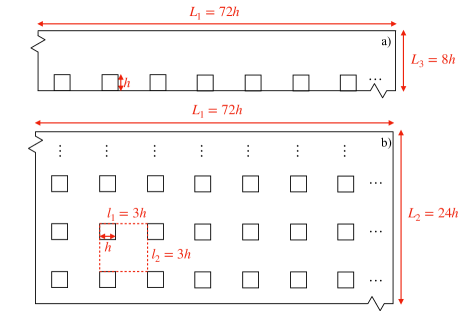
Figure 1: Side and planar view of the computational domain (a and b respectively). The red dashed line denotes the repeating unit.

Two LESs of flow over an array of surface-mounted cubes are carried out. The two simulations only differ by the pressure forcing term: One is characterized by a pressure gradient that is constant in space and time (CP hereafter), and the other by a pressure gradient that is constant in space and pulsatile in time (PP).

The computational domain for both simulations is sketched in figure 1. The size of the box is $[0,L_{1}]\times[0,L_{2}]\times[0,L_{3}]$ with $L_{1}=72h$, $L_{2}=24h$, and $L_{3}=8h$, where $h$ denotes the height of cubes. Cubes are organized in an in-line arrangement with planar and frontal area fractions set to $\lambda_{p}=\lambda_{f}=0.\overline{1}$. The relatively high packing density and the relatively large scale separation $L_{3}/h$ support the existence of an inertial sublayer in the considered flow system (Coceal et al., 2007; Castro, 2007; Zhang et al., 2022). In terms of horizontal extent, $L_{1}/L_{3}$ and $L_{2}/L_{3}$ are larger than those from previous works focusing on coherent structures above aerodynamically rough surfaces (Coceal et al., 2007; Xie et al., 2008; Leonardi & Castro, 2010; Anderson et al., 2015b) and are sufficient to accommodate large-scale motions (Balakumar & Adrian, 2007). An aerodynamic roughness length $z_{0}=10^{-4}h$ is prescribed at the cube surfaces and the ground, via the algebraic wall-layer model, resulting in negligible SGS drag contributions to the total surface drag (Yang & Meneveau, 2016). The computational domain is discretized using a uniform Cartesian grid of $N_{1}\times N_{2}\times N_{3}=576\times 192\times 128$, so each cube is resolved by $8\times 8\times 16$ grid points. Such a grid resolution yields flow statistics that are poorly sensitive to grid resolution in both statistically stationary and pulsatile flows at the considered oscillation frequency (Tseng et al., 2006; Li & Giometto, 2022).

For the PP case, the chosen forcing amplitude and frequency are $\alpha_{p}=12$ and $\omega T_{\mathrm{h}}=\pi/8$, respectively, where $T_{\mathrm{h}}=h/u_{\tau}$ is the averaged turnover time of characteristic eddies of the urban canopy layer (UCL) and ${u}_{\tau}=\sqrt{f_{m}L_{3}}$ is the friction velocity. In dimensional terms, considering realistic values of the friction velocity and UCL height in the ABL, i.e., $0.1\leq{u}_{\tau}\leq 0.5\ \rm{m/s}$ and $3\leq h\leq 30\ \rm{m}$ (Stull, 1988), the considered frequency corresponds a time period $24\leq T\leq 4800\ \rm{s}$. This range of time scales pertains to sub-mesoscale motions (Mahrt, 2009; Hoover et al., 2015), which, as outlined in §1, are a major driver of atmospheric pressure gradient variability. In addition, as demonstrated in Li & Giometto (2022), the current flow system exhibits a Stokes layer, where turbulence generation and momentum transport are considerably modified during the pulsation cycle. The selected frequency produces a Stokes layer thickness of $\delta_{s}=5h$, indicating that the roughness sublayer (RSL) and inertial sublayer (ISL) are both affected by the non-stationarity. To focus on the current-dominated flow regime, we choose a value of $\alpha_{p}=12$, which is large enough to induce significant changes in the coherent structures with the varying pressure gradient while avoiding mean flow reversals.

Both simulations are initialized with velocity fields from a stationary flow case and integrated over $400T_{atm}$, corresponding to $200$ pulsatile cycles for the PP case. Here $T_{atm}=L_{3}/{u}_{\tau}$ refers to the turnover time of the largest eddies in the domain. The size of time step is set to $\delta t=5\cdot 10^{-5}T_{atm}$ which satisfies the Courant-Friedrichs-Lewy stability condition, i.e., $\max{(CFL)}=u_{max}\delta t/\delta\approx 0.05$, where $u_{max}$ is the maximum velocity magnitude at any point in the domain during the simulation, and $\delta$ is the size of the grid stencil, $\delta t$ being the size of the time step. The initial $20T_{atm}$ are discarded for both the CP and PP cases (transient period for the PP case), which correspond to about 10 oscillation periods, after which instantaneous snapshots of velocities and pressure are collected and saved every $0.025T_{atm}$ ($1/80$ of the pulsatile cycle).

2.3 Notation and terminology

For the PP case, $\overline{(\cdot)}$ denotes an ensemble averaging operation, performed over the phase dimension and over repeating surface units (see figure 1), i.e., for a given flow quantity $\theta$,

$$\overline{\theta}(x_{1},x_{2},x_{3},t)=\frac{1}{N_{p}n_{1}n_{2}}\sum^{N_{p}}_{n=1}\sum^{n_{1}}_{i=1}\sum^{n_{2}}_{j=1}\theta(x_{1}+il_{1},x_{2}+jl_{2},x_{3},t+nT),\\ 0\leq x_{1}\leq l_{1},\quad 0\leq x_{2}\leq l_{2},\quad 0\leq t\leq T\ .$$ (3)

Using the usual Reynolds decomposition, one can write

$$\theta(x_{1},x_{2},x_{3},t)=\overline{\theta}(x_{1},x_{2},x_{3},t)+\theta^{\prime}(x_{1},x_{2},x_{3},t)\ \,$$ (4)

where $(\cdot)^{\prime}$ denotes a fluctuation from the ensemble average. For the CP case, $\overline{(\cdot)}$ denotes a quantity averaged over repeating units only. An ensemble averaged quantity can be further decomposed into an intrinsic spatial average and a deviation from the intrinsic average (Schmid et al., 2019), i.e.,

$$\overline{\theta}(x_{1},x_{2},x_{3},t)=\langle\overline{\theta}\rangle(x_{3},t)+\overline{\theta}^{\prime\prime}(x_{1},x_{2},x_{3},t)\ .$$ (5)

Note that, for each $x_{3}$, the intrinsic averaging operation is taken over a thin horizontal “slab” $V_{f}$ of fluid, characterized by a thickness $\delta_{3}$ in the wall-normal ($x_{3}$) direction, namely,

$$\langle\overline{\theta}\rangle(x_{3},t)=\frac{1}{V_{f}}\int_{x_{3}-\delta_{3}/2}^{x_{3}+\delta_{3}/2}\int_{0}^{L_{2}}\int_{0}^{L_{1}}\overline{\theta}(x_{1},x_{2},x_{3},t)dx_{1}dx_{2}dx_{3}\ .$$ (6)

Further, any phase-averaged quantity from the PP case consists of a longtime-averaged component and an oscillatory component with a zero mean, which will be hereafter denoted via the subscripts $l$ and $o$, respectively, i.e.,

$$\overline{\theta}(x_{1},x_{2},x_{3},t)=\overline{\theta}_{l}(x_{1},x_{2},x_{3})+\overline{\theta}_{o}(x_{1},x_{2},x_{3},t)$$ (7)

and

$$\langle\overline{\theta}\rangle(x_{3},t)=\langle\overline{\theta}\rangle_{l}(x_{3})+\langle\overline{\theta}\rangle_{o}(x_{3},t)\ .$$ (8)

As for the CP case, the longtime and ensemble averages are used interchangeably due to the lack of an oscillatory component. In the following, the longtime-averaged quantities from the PP case are contrasted against their counterparts from the CP case to highlight the impact of flow unsteadiness on flow characteristics in a longtime average sense. Oscillatory and phase-averaged quantities are analyzed to shed light on the phase-dependent features of the PP case.

3 Results

3.1 Overview of flow statistics

Li & Giometto (2022) have proposed a detailed analysis of pulsatile flow over an array of surface-mounted cuboids, discussing the impact of varying forcing amplitude and frequency on selected flow statistics. Here, we repropose and expand upon some of the findings that are relevant to this work.

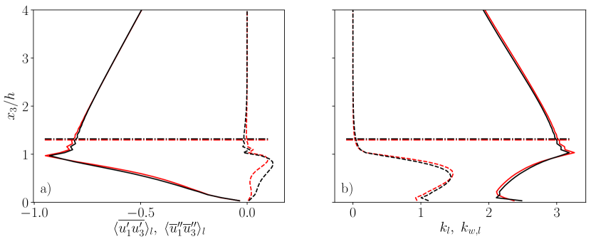
Figure 2: (a) Longtime-averaged shear stresses normalized by ${u}_{\tau}$ from the PP (black) and CP (red) cases. Resolved Reynolds shear stress $\langle\overline{u^{\prime}_{1}u^{\prime}_{3}}\rangle_{l}$, solid lines; dispersive shear stress $\langle\overline{u}^{\prime\prime}_{1}\overline{u}^{\prime\prime}_{3}\rangle_{l}$. (b) Longtime-averaged turbulent and wake kinetic energy from the PP (black) and CP (red) cases. Resolved turbulent kinetic energy $k_{l}=\langle\overline{u^{\prime}_{i}u^{\prime}_{i}}\rangle_{l}/2$, solid lines; wake kinetic energy $k_{w,l}=\langle\overline{u}^{\prime\prime}_{i}\overline{u}^{\prime\prime}_{i}\rangle_{l}/2$, dashed lines. Dashed-dotted horizontal lines denote the upper bound of the RSL $(\delta_{RSL})$.

Figure 2(a) presents the wall-normal distributions of the longtime-averaged resolved Reynolds shear stress $\langle\overline{u^{\prime}_{1}u^{\prime}_{3}}\rangle_{l}$ and dispersive shear stress $\langle\overline{u}^{\prime\prime}_{1}\overline{u}^{\prime\prime}_{3}\rangle_{l}$. Note that SGS components contribute $<1\%$ to the total Reynolds stress, and are hence not discussed. From the figure, it is apparent that flow unsteadiness does not noticeably affect the $\langle\overline{u^{\prime}_{1}u^{\prime}_{3}}\rangle_{l}$ profile, which is characterized by $<3\%$ departures from the statistically stationary case. On the contrary, flow pulsation within the UCL leads to pronounced increases in $\langle\overline{u}^{\prime\prime}_{1}\overline{u}^{\prime\prime}_{3}\rangle_{l}$ (up to 500% locally). However, despite this increase, the dispersive flux remains a modest contributor to the total momentum flux in the UCL. Figure 2(b) displays the longtime-averaged resolved turbulent kinetic energy $k_{l}=\langle\overline{u^{\prime}_{i}u^{\prime}_{i}}\rangle_{l}/2$ and wake kinetic energy $k_{w,l}=\langle\overline{u}^{\prime\prime}_{i}\overline{u}^{\prime\prime}_{i}\rangle_{l}/2$. Both $k_{l}$ and $k_{w,l}$ from the PP case feature modest departures from their CP counterparts (discrepancies are $<5\%$), highlighting a weak dependence of both longtime-averaged turbulent and wake kinetic energy on flow unsteadiness. Also, the RSL thicknesses $\delta_{RSL}$ for the CP and PP cases are depicted in figure 2. Following the approach by Pokrajac et al. (2007), $\delta_{RSL}$ is estimated by thresholding the spatial standard deviation of the longtime-averaged streamwise velocity normalized by its intrinsic average, namely,

$$\sigma=\frac{\sqrt{\langle(\overline{u}_{1,l}-\langle\overline{u}_{1}\rangle_{l})^{2}\rangle}}{\langle\overline{u}_{1}\rangle_{l}}\ ,$$ (9)

where the threshold is taken as 1%. An alternative method to evaluate $\delta_{RSL}$ involves using phase-averaged statistics instead of long-time-averaged ones in (9). Although now shown, such a method yields similar predictions (with a discrepancy of less than $5\%$). Both $\langle\overline{u}^{\prime\prime}_{1}\overline{u}^{\prime\prime}_{3}\rangle_{l}$ and $k_{w,l}$, which result from spatial variations of time-averaged flow quantities, reduce to $<1\%$ of their peak value above $\delta_{RSL}$. From figure 2, one can readily observe that flow unsteadiness increases the extent of the RSL, with estimated $\delta_{RSL}$s not exceeding $1.5h$ in both cases. Hereafter, we will assume $\delta_{RSL}=1.5h$. As discussed in §1, RSL and ISL feature distinct coherent structures. Specifically, the structures in the RSL are expected to show strong imprints of roughness elements, whereas those in the ISL should, in principle, be independent of surface morphology (Coceal et al., 2007).

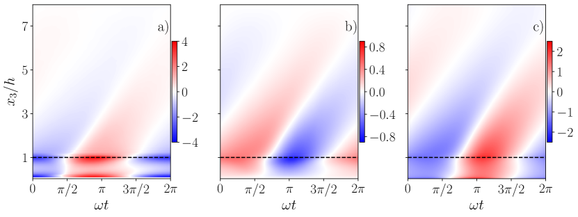
Figure 3: Space-time diagrams of (a) oscillatory shear rate ${\partial\langle\overline{u}_{1}\rangle_{o}}/{\partial x_{3}}$, (b) oscillatory resolved Reynolds shear stress $\langle\overline{u_{1}^{\prime}u_{3}^{\prime}}\rangle_{o}$, and (c) oscillatory resolved turbulent kinetic energy $k_{o}=\langle\overline{u^{\prime}_{i}u^{\prime}_{i}}\rangle_{o}/2$ from the PP case. Results are normalized by $u_{\tau}$ and $h$. Horizontal dashed lines highlight the top of the UCL.

The response of first- and second-order flow statistics to flow unsteadiness are depicted in figure 3. Figure 3(a) highlights the presence of an oscillating wave in the oscillatory shear rate $\langle{\partial\overline{u}_{1}}/{\partial x_{3}}\rangle_{o}$ generated at the canopy top in response to the flow unsteadiness, with a $\pi/2$ phase lag respective to the pulsatile pressure forcing. Such a wave propagates in the positive vertical direction while being attenuated and diffused by turbulent friction and mixing. It is noteworthy that the propagation speed of the oscillating shear rate is constant, as suggested by the constant tilting angle along the $x_{3}$ direction in the $\langle{\partial\overline{u}}/{\partial x_{3}}\rangle_{o}$ contour. As apparent from figure 3(b,c), the space-time diagrams of the oscillatory resolved Reynolds shear stress $\langle\overline{u_{1}^{\prime}u_{3}^{\prime}}\rangle_{o}$ and oscillatory resolved turbulent kinetic energy $k_{o}=\langle\overline{u^{\prime}_{i}u^{\prime}_{i}}\rangle_{o}/2$ are also characterized by decaying waves traveling away from the RSL at constant speeds. The speeds of these waves are similar to that of the corresponding oscillating shear rate, which can be inferred by the identical tilting angles in the contours. There is clearly a causal relation for this behavior: above the UCL, the major contributors of shear production terms in the budget equations of $\langle\overline{u_{1}^{\prime}u_{3}^{\prime}}\rangle_{o}$ and $k_{o}$ are

$$\langle\overline{\mathcal{P}}\rangle_{13,o}=-\langle\overline{u_{3}^{\prime}u_{3}^{\prime}}\rangle_{l}\langle\frac{\partial\overline{u}}{\partial x_{3}}\rangle_{o}-\langle\overline{u_{3}^{\prime}u_{3}^{\prime}}\rangle_{o}\langle\frac{\partial\overline{u}}{\partial x_{3}}\rangle_{l}\ ,$$ (10)

and

$$\langle\overline{\mathcal{P}}\rangle_{k,o}=-2\langle\overline{u_{1}^{\prime}u_{3}^{\prime}}\rangle_{l}\langle\frac{\partial\overline{u}}{\partial x_{3}}\rangle_{o}-2\langle\overline{u_{1}^{\prime}u_{3}^{\prime}}\rangle_{o}\langle\frac{\partial\overline{u}}{\partial x_{3}}\rangle_{l}\ ,$$ (11)

respectively. As the oscillating shear rate travels upwards away from the UCL, it interacts with the local turbulence by modulating $\langle\overline{\mathcal{P}}\rangle_{13,o}$ and $\langle\overline{\mathcal{P}}\rangle_{k,o}$, and ultimately yielding the observed oscillations in resolved Reynolds stresses. On the other hand, no pulsatile-forcing-related terms appear in the budget equations of resolved Reynolds stresses. This indicates that the oscillating shear rate induced by the pulsatile forcing modifies the turbulence production above the UCL rather than the pressure forcing itself. A similar point about pulsatile flows was made in Scotti & Piomelli (2001), where it was stated that “[…] in the former [pulsatile flow] it is the shear generated at the wall that affects the flow”. It is worth noting that such a study was however based on pulsatile flow over smooth surfaces and at a relatively low Reynolds number.

In addition, a visual comparison of the contours of $\langle{\partial\overline{u}}/{\partial x_{3}}\rangle_{o}$ and $-\langle\overline{u_{1}^{\prime}u_{3}^{\prime}}\rangle_{o}$ highlights the presence of a phase lag between $\langle{\partial\overline{u}}/{\partial x_{3}}\rangle_{o}$ and $-\langle\overline{u_{1}^{\prime}u_{3}^{\prime}}\rangle_{o}$. That is to say, the turbulence is not in equilibrium with the mean flow during the pulsatile cycle, even though the pulsatile forcing or the induced oscillating shear wave does not substantially modify the longtime-averaged turbulence intensity (see figure 2). To gain further insight into this behavior, the next section examines the structure of turbulence under the considered non-equilibrium condition.

3.2 Quadrant analysis

The discussions will first focus on the impact of flow pulsation on $u_{1}^{\prime}u_{3}^{\prime}$ quadrants. This statistical analysis will allow us to quantify the contributions of different coherent motions to the turbulent momentum transport. The quadrant analysis technique was first introduced by Wallace et al. (1972), and has thereafter been routinely employed to characterize the structure of turbulence across a range of flow systems (Wallace, 2016). The approach maps velocity fluctuations to one of four types of coherent motions (quadrants) in the $u_{1}^{\prime}-u_{3}^{\prime}$ phase space, namely,

$$\begin{cases}Q1:&u_{1}^{\prime}>0,u_{3}^{\prime}>0\\ Q2:&u_{1}^{\prime}<0,u_{3}^{\prime}>0\\ Q3:&u_{1}^{\prime}<0,u_{3}^{\prime}<0\\ Q4:&u_{1}^{\prime}>0,u_{3}^{\prime}<0\ .\end{cases}$$ (12)

Q2 and Q4 are typically referred to as ejections and sweeps, respectively. They are the main contributors to the Reynolds shear stress, and compose the majority of the events in boundary layer flows. Ejections are associated with the lift-up of low-momentum fluid by vortex induction between the legs of hairpin structures, whereas sweeps correspond to the down-draft of the high-momentum fluid (Adrian et al., 2000). Q1 and Q3 denote outward and inward interactions, and play a less important role in transporting momentum compared to Q2 and Q4. Coceal et al. (2007) and Finnigan (2000) showed that the RSL of stationary flows is dominated by ejections in terms of events, but that the overall Reynolds stress contribution from sweeps stress exceeds that from ejections. Away from the RSL, the trend is the opposite. This behavior is indeed apparent from figure 4, where ejection and sweep profiles are shown for the CP case (red lines).

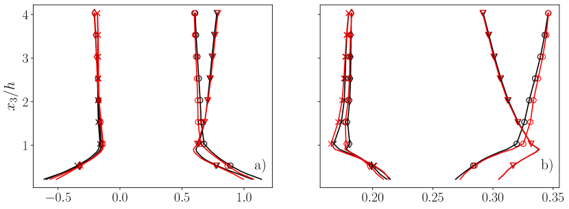
Figure 4: (a) Relative contribution to $\overline{u_{1}^{\prime}u_{3}^{\prime}}$ by events in each quadrant summed over the wall-parallel planes and the whole sampling time period and (b) relative number of events in each quadrant from the PP case (black) and CP (red) as a function of $x_{3}$. Cross: outward interaction; triangles: ejection; diamonds: inward interaction; circles: sweep.

We first examine the overall frequency of events in each quadrant and the contribution of each quadrant to the resolved Reynolds shear stress. For the considered cases, the contribution to $\overline{u_{1}^{\prime}u_{3}^{\prime}}$ and the number of the events of each quadrant are summed over different wall-parallel planes and over the whole sampling time period (i.e., these are longtime-averaged quantities). Results from this operation are shown in figure 4. What emerges from this figure is that flow pulsation does not significantly alter the relative contribution and frequency of each quadrant. Some discrepancies between CP and PP profiles can be observed immediately above the UCL, but do not sum to more than 4% at any given height.

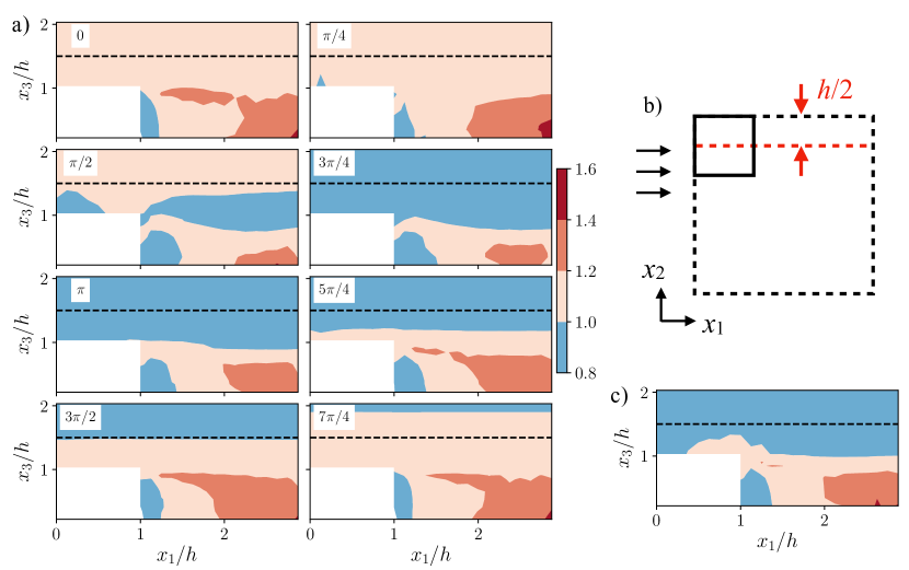
Figure 5: (a) Ratio between the numbers of ejections to sweeps ($\gamma_{\#}$) from the PP case at a streamwise/wall-normal plane. (b) Location of the selected streamwise/wall-normal plane (red dashed line) within a repeating unit. (c) $\gamma_{\#}$ from the CP case at the same plane. Black dashed lines denote $x_{3}/h=1.5$, where is the upper limit of the RSL.

Next, we shed light on the phase-dependent features of quadrant distributions with a focus on sweeps and ejections, as it has been shown that they are the major contributors to the momentum flux (see figure 4). Hereafter the ratio between the numbers of ejections and sweeps is denoted by $\gamma_{\#}$, and the ratio of the contribution to $\overline{u_{1}^{\prime}u_{3}^{\prime}}$ is represented by $\gamma_{c}$. Note that as mentioned in the previous section, a turbulence fluctuation is defined as a deviation from the local ensemble average, so the number of occurrences and contribution to $\overline{u_{1}^{\prime}u_{3}^{\prime}}$ of each quadrant are functions of both the location relative to the cube within the repeating unit and the phase for the PP case, and so are $\gamma_{\#}$ and $\gamma_{c}$. Conversely, in the CP case, $\gamma_{\#}$ and $\gamma_{c}$ are only functions of the spatial location relative to the cube. Figure 5(a) and (c) present $\gamma_{\#}$ up to $x_{3}/h=2$ at a selected streamwise/wall-normal plane for the PP and CP cases, respectively. The chosen plane cuts through the center of a cube in the repeating unit, as shown in 5(b). In the cavity, the ejection-sweep pattern from the PP case is found to be qualitative similar to its CP counterpart throughout the pulsatile cycle (compare subplots (a) and (c) in figure 5). Specifically, a preponderance of sweeps characterizes a narrow region in the leeward side of the cube (the streamwise extent of this region is $\lessapprox 0.3h$), whereas ejections dominate in the remainder of the cavity. As also apparent from figure 5(a), the streamwise extent of the sweep-dominated region increases (decreases) during the acceleration (deceleration) time period. During the acceleration phase, the $h<x_{3}<2h$ region (i.e., immediately above the UCL) transitions from an ejection-dominated flow regime to a sweep-dominated one, and vice versa as the flow decelerates. Such a transition first occurs immediately above the cavity, where a larger amount of sweeps (ejections) are generated during the acceleration (deceleration) period, until they populate in the whole RSL. Although not presented here, $\gamma_{c}$ features an exactly opposite trend.

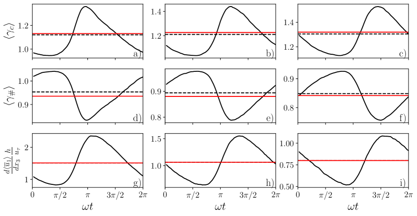
Figure 6: (a) - (c): Intrinsic-averaged ratio of contributions to $\overline{u_{1}^{\prime}u_{3}^{\prime}}$ from ejections and sweeps ($\langle\gamma_{c}\rangle$); (d) - (f): intrinsic-averaged ratio of ejections to sweeps ($\langle\gamma_{\#}\rangle$); (g) - (i): phase-averaged shear rate ${\partial\langle\overline{u}_{1}\rangle}/{\partial x_{3}}$ from the PP case at three wall-normal locations within the ISL (a,d,g) $x_{3}/h=2$, (b,e,h) $x_{3}/h=3$, and (c,f,i) $x_{3}/h=4$ as a function of phase. Black dashed lines denote longtime-averaged values, whereas solid red lines represent corresponding quantities from the CP case.

Shifting the attention to the ejection-sweep pattern in the ISL, figure 6 shows the intrinsic average of $\gamma_{c}$ and $\gamma_{\#}$ at the $x_{3}/h=\{2,3,4\}$ planes. These quantities are hereafter denoted as $\langle\gamma_{c}\rangle$ and $\langle\gamma_{\#}\rangle$, respectively. The use of $\langle\gamma_{c}\rangle$ and $\langle\gamma_{\#}\rangle$ instead of $\gamma_{c}$ and $\gamma_{\#}$ to characterize the ejection-sweep pattern in the ISL can be justified by the fact that the spatial variations in $\gamma_{\#}$ and $\gamma_{c}$ on the wall-parallel directions vanish rapidly above the RSL, as apparent from figure 5. This is in line with the observations of Kanda et al. (2004) and Castro et al. (2006) that the spatial variations in $\gamma_{\#}$ and $\gamma_{c}$ are concentrated in the RSL for stationary flow over urban canopy. The ejection-sweep pattern varies substantially during the pulsatile cycle. For example, at $x_{3}/h=2$, even though the contribution from the ejections to $\overline{u_{1}^{\prime}u_{3}^{\prime}}$ dominates in a longtime average sense, i.e., $\langle\gamma_{c}\rangle_{l}>1$, the flow features $\langle\gamma_{c}\rangle<1$ for $\omega t\in[0,\approx\pi/2]$ (see figure 6,a). More interestingly, this ejection-sweep pattern at a given wall-normal location appears to be directly controlled by the phase-averaged shear rate ${\partial\langle\overline{u}_{1}\rangle}/{\partial x_{3}}$, as elaborated in the following. As ${\partial\langle\overline{u}_{1}\rangle}/{\partial x_{3}}$ increases at a given $x_{3}$, the corresponding $\langle\gamma_{c}\rangle$ increases whereas $\langle\gamma_{\#}\rangle$ decreases, highlighting the presence of fewer but stronger ejections events. The absolute maximum (minimum) of $\langle\gamma_{c}\rangle$ ($\langle\gamma_{\#}\rangle$) approximately coincides with the maximum (minimum) of ${\partial\langle\overline{u}_{1}\rangle}/{\partial x_{3}}$. This observation is consistent across the considered planes. As discussed in the next sections, such behavior can be attributed to time variations in the geometry of ISL structures.

3.3 Spatial and temporal flow coherence

To gain a better understanding of the extent and organization of coherent structures in the ISL, this section analyzes two-point velocity autocorrelation maps. This flow statistic provides information on the linear correlation of the flow field in space, making it an effective tool for describing spatial flow coherence (Dennis & Nickels, 2011; Guala et al., 2012).

For the PP case, the phase-dependent two-point correlation coefficient tensor $\overline{R}_{ij}$ can be defined as

$$\overline{R}_{ij}(\Delta_{1},\Delta_{2},x_{3},x_{3}^{*},t)=\frac{\langle\overline{u_{i}^{\prime}(x_{1},x_{2},x_{3}^{*},t)u_{j}^{\prime}(x_{1}+\Delta_{1},x_{2}+\Delta_{2},x_{3},t)}\rangle}{\sqrt{\langle\overline{u_{i}^{\prime}u_{i}^{\prime}}\rangle(x_{3}^{*},t)\langle\overline{u_{j}^{\prime}u_{j}^{\prime}}\rangle(x_{3},t)}}\ ,$$ (13)

where $\Delta_{i}$ is the separation on the wall-parallel directions, $x_{3}^{*}$ represents a reference wall-normal location, and $t$ denotes the phase. In the CP case, the flow is statistically stationary, and therefore $\overline{R}_{ij}$ is not a function of $t$, i.e., $\overline{R}_{ij}=\overline{R}_{ij,l}$.

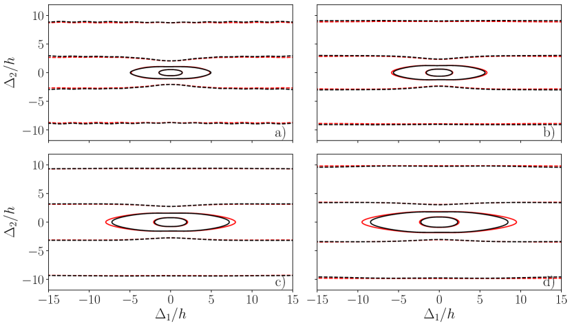
Figure 7: Longtime-averaged two-point correlation coefficient tensor $\overline{R}_{11,l}$ at (a) $x_{3}^{*}/h=1.5$, (b) $x_{3}^{*}/h=2$, (c) $x_{3}^{*}/h=3$, and (d) $x_{3}^{*}/h=4$. Black lines correspond to the PP case, and red lines to the CP one. $\overline{R}_{11,l}=0.6$ and $\overline{R}_{11,l}=0.3$ are denoted by solid lines, and dashed lines represent $\overline{R}_{11,l}=0$.

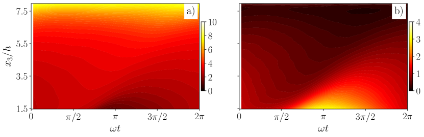
Figure 8: Time evolution of (a) the cross-stream streak width normalized by $h$ and (b) $\partial\langle\overline{u}_{1}\rangle/\partial x_{3}$. The cross-stream width is identified as the first zero crossing of the $\overline{R}_{11}=0$ field.

Figure 7 compares $\overline{R}_{11,l}$ for the PP and CP cases over the $x_{3}^{*}/h=\{1.5,2,3,4\}$ planes. In both cases, $\overline{R}_{11,l}$ features an alternating sign in the cross-stream direction, signaling the presence of low- and high-momentum streaks flanking each other in the cross-stream direction. The cross-stream extent of longtime-averaged streaks can be identified as the first zero-crossing of the $\overline{R}_{11,l}$ contour in the $\Delta_{2}$ direction. Based on this definition, figure 7 shows that flow unsteadiness has a modest impact on such a quantity. This finding agrees with observations from Zhang & Simons (2019) for pulsatile flow over smooth surfaces. Further, although not shown, the streamwise and cross-stream extent of streaks increases linearly in $x_{3}$, suggesting that Townsend’s attached-eddy hypothesis is valid in a longtime average sense (Marusic & Monty, 2019).

Turning the attention to the phase-averaged flow field, figure 8 shows the time variation of the cross-stream streaks extent, which is identified as the first zero crossing of the $\overline{R}_{11}=0$ field in the cross-stream direction. The linear $x_{3}$-scaling of the streak width breaks down in a phase-averaged sense. Such a quantity indeed varies substantially during the pulsatile cycle, diminishing in magnitude as ${\partial\langle\overline{u}_{1}\rangle}/{\partial x_{3}}$ increases throughout the boundary layer. Interestingly, when ${\partial\langle\overline{u}_{1}\rangle}/{\partial x_{3}}$ reaches its maximum at $\omega t\approx\pi$ and $x_{3}/h\approx 1.5$, the cross-stream extent of streaks approaches zero, suggesting that streaks may not be a persistent feature of pulsatile boundary layer flows.

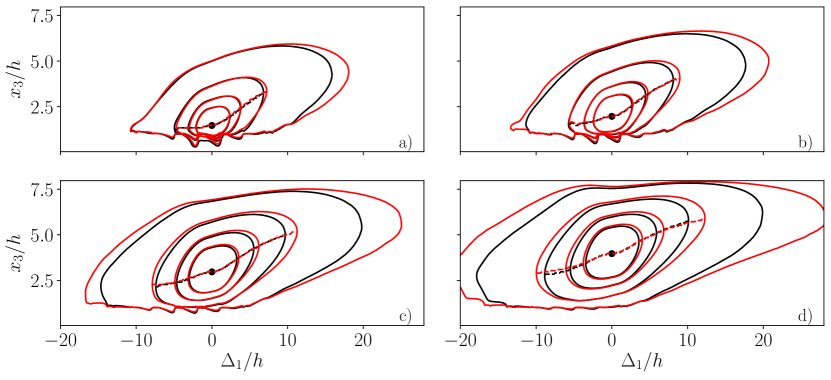
Figure 9: $\overline{R}_{11,l}$ in the streamwise/wall-normal plane of the PP (black) and CP (red) cases. Results correspond to four reference wall-normal locations: (a) $x_{3}^{*}/h=1.5$, (b) $x_{3}^{*}/h=2$, (c) $x_{3}^{*}/h=3$, and (d) $x_{3}^{*}/h=4$. Contour levels (solid lines) range from $0.2$ to $0.5$ with increments of $0.1$. Dashed lines denote the locus of the maximum correlation at each streamwise location. The slopes of the dashed lines represent the tilting angles of the structures.

To further quantify topological changes induced by flow pulsation, we hereafter examine variations in the streamwise and wall-normal extent of coherent structures. Such quantities will be identified via the $\overline{R}_{11}=0.3$ contour, in line with the approach used by Krogstad & Antonia (1994). Note that the choice of the $\overline{R}_{11}$ threshold for such a task is somewhat subjective, and several different values have been used in previous studies to achieve this same objective, including $\overline{R}_{11}=0.4$ (Takimoto et al., 2013) and $\overline{R}_{11}=0.5$ (Volino et al., 2007; Guala et al., 2012). In this study, the exact threshold is inconsequential as it does not impact the conclusions. Figure 9 presents $\overline{R}_{11,l}$ contours in the streamwise/wall-normal plane for $x_{3}^{*}/h=\{1.5,2,3,4\}$. The jagged lines at $x_{3}/h\approx 1$ (the top of the UCL) bear the signature of roughness elements. The dashed lines passing through $x_{3}^{*}$ identify the locus of the maxima in $\overline{R}_{11,l}$ at each streamwise location. The inclination angle of such lines can be used as a surrogate for the longtime-averaged tilting angle of the coherent structure (Chauhan et al., 2013; Salesky & Anderson, 2020). It is clearly observed that at each reference wall-normal location, the tilting angle of longtime-averaged structures is similar between the PP case and CP. The tilting angle in both cases decreases monotonically and slowly from $15^{\circ}$ at $x_{3}^{*}/h=1.5$ to $10^{\circ}$ at $x_{3}^{*}/h=4$—a behavior that is in excellent agreement with results from Coceal et al. (2007), even though a different urban canopy layout was used therein. Further, the identified tilting angle is similar to the one inferred from real-world ABL observations in Hutchins et al. (2012) and Chauhan et al. (2013). On the other hand, longtime-averaged coherent structures in the PP case are relatively smaller than in the CP case in both the streamwise and wall-normal coordinate directions. Discrepancies become more apparent with increasing $x_{3}^{*}$. The difference in the streamwise (wall-normal) extent of the longtime-averaged structure from the two cases increases from $2\%$ ($2\%$) at $x_{3}^{*}/h=1.5$ to $15\%$ ($4\%$) at $x_{3}^{*}/h=4$. From the above analysis, it is hence apparent that flow pulsation reduces the streamwise and wall-normal extents of the longtime-averaged coherent structure while preserving their inclination angle.

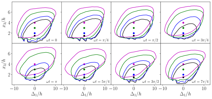
Figure 10: Time evolution of $\overline{R}_{11}=0.3$ in the streamwise/wall-normal plane. Line colors denote the contours corresponding to different $x_{3}^{*}$ planes: $x_{3}^{*}/h=1.5$ (black), $x_{3}^{*}/h=2$ (blue), $x_{3}^{*}/h=3$ (green), and $x_{3}^{*}/h=4$ (magenta). Dots highlight the location of the reference plane.

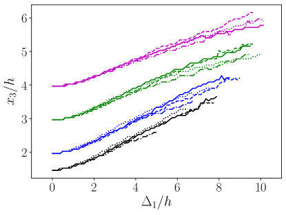
Figure 11: The locus of the maximum $\overline{R}_{11}$ at four phases: $\omega t=0$ (solid lines), $\omega t=\pi/2$ (dashed lines), $\omega t=\pi$ (dashed dotted lines), and $\omega t=3\pi/2$ (dotted lines). Line colors denote different reference elevations: $x_{3}^{*}/h=1.5$ (black), $x_{3}^{*}/h=2$ (blue), $x_{3}^{*}/h=3$ (green), and $x_{3}^{*}/h=4$ (magenta).

More insight into the mechanisms underpinning the observed behavior can be gained by examining the time evolution of such structures for the PP case in figure 10. When taken together with figure 8(b), it becomes clear that both the streamwise and the wall-normal extents of the coherent structures tend to reduce with increasing local $\partial\langle\overline{u}_{1}\rangle/\partial x_{3}$. Compared to the streamwise extent, the wall-normal extent of the coherent structure is more sensitive to changes in $\partial\langle\overline{u}_{1}\rangle/\partial x_{3}$. For example, at $x_{3}^{*}/h=4$, we observe an overall $15\%$ variation in the wall-normal extent of the coherent structure during a pulsation cycle, whereas the corresponding variation in streamwise extent is $8\%$. Further, the phase-averaged $\overline{u}_{1}$ field at the considered heights appears to be more correlated with the flow in the UCL for small $\partial\langle\overline{u}_{1}\rangle/\partial x_{3}$, thus highlighting a stronger coupling between flow regions. Interestingly, the tilting angle of the coherence structure remains constant during the pulsatile cycle, as shown in figure 11.

Next, we will show that the hairpin vortex packet paradigm (Adrian, 2007) can be used to provide an interpretation for these findings. The validity of such a paradigm is supported by a vast body of evidence, including laboratory experiments of canonical TBL (Adrian et al., 2000; Christensen & Adrian, 2001; Dennis & Nickels, 2011) to ABL field measurements (Hommema & Adrian, 2003; Morris et al., 2007) and numerical simulations (Lee et al., 2011; Eitel-Amor et al., 2015). This formulation assumes that the dominant ISL structures are hairpin vortex packets, consisting of a sequence of hairpin vortices organized in a quasi-streamwise direction with a characteristic inclination angle relative to the wall. These structures encapsulate the low-momentum regions, also known as “streaks”. The observed changes in $\overline{R}_{11,l}$ between the CP and PP cases and of $\overline{R}_{11}$ contours during the pulsatile cycle reflect corresponding changes in the geometry of vortex packets in a longtime- and phase-averaged sense. Specifically, as $\partial\langle\overline{u}_{1}\rangle/\partial x_{3}$ increases, the phase-averaged size of vortex packets is expected to shrink, and, in the longtime-averaged sense, the vortex packets are smaller than their counterparts in the CP case. However, upon inspection of $R_{11}$, it is unclear whether the observed change in packet size is attributable to variations in the composing hairpin vortices or the tendency for packets to break into smaller ones under high $\partial\langle\overline{u}_{1}\rangle/\partial x_{3}$ and merge into larger ones under low $\partial\langle\overline{u}_{1}\rangle/\partial x_{3}$. To answer this question, we will examine the instantaneous turbulence structures and extract characteristic hairpin vortices through conditional averaging in the following sections. Also, the constant tilting angle of the structure during the pulsatile cycle indicates that, no matter how vortex packets break and reorganize and how individual hairpin vortices deform in response to the time-varying shear rate, the hairpin vortices within the same packet remain aligned with a constant tilting angle.

3.4 Instantaneous flow structure

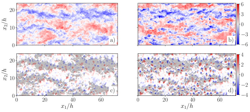
Figure 12: (a, b): Instantaneous fluctuating streamwise velocity $u_{1}^{\prime}$ normalized by ${u}_{\tau}$; (c, d): wall-normal swirl strength $\lambda_{s,3}$ of the PP case at $x_{3}=2h$. (a, c): $\omega t=\pi/2$, ; (b, d), $\omega t=\pi$. Shaded regions in (c, d) highlight the low-momentum ($u_{1}^{\prime}<0$) regions. The instantaneous flow fields are obtained from the same pulsatile cycle.

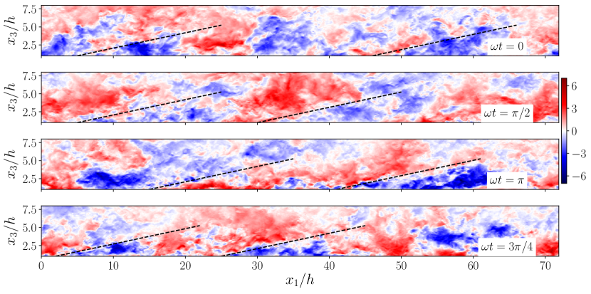
Figure 13: Instantaneous fluctuating streamwise velocity $u_{1}^{\prime}$ in a streamwise/wall-normal plane during a pulsatile cycle. Black dashed lines denote the $12^{\circ}$ structural tilting angle of the coherent structure.

Figure 12(a) and (b) show the instantaneous fluctuating streamwise velocity $u_{1}^{\prime}$ at $x_{3}/h=1.5$ from the PP case. The chosen phases, $\omega t=\pi/2$ and $\omega t=\pi$, correspond to the local minimum and maximum of $\partial\langle\overline{u}_{1}\rangle/\partial x_{3}$, respectively (see figure 6,g). Streak patterns can be observed during both phases. As shown in figure 12(a), at low $\partial\langle\overline{u}_{1}\rangle/\partial x_{3}$ values, instantaneous $u_{1}^{\prime}$ structures intertwine with neighboring ones, and form large streaks with a cross-stream extent of about $5h$. Conversely, when $\partial\langle\overline{u}_{1}\rangle/\partial x_{3}$ is large, streaks are scrambled into smaller structures, characterized by a cross-stream extent of about $h$. This behavior is consistent with the observations we made based on figure 8. Figure 12(c) and (d) depict the corresponding low-pass filtered wall-normal swirl strength $\lambda_{s,3}$. The definition of the signed planar swirl strength $\lambda_{s,i}$ is based on the studies of Stanislas et al. (2008) and Elsinga et al. (2012). The magnitude of $\lambda_{s,i}$ is the absolute value of the imaginary part of the eigenvalue of the reduced velocity gradient tensor $J_{jk}$, which is

$$J_{jk}=\begin{bmatrix}{\partial u_{j}}/{\partial x_{j}}&{\partial u_{j}}/{\partial x_{k}}\\ {\partial u_{k}}/{\partial x_{j}}&{\partial u_{k}}/{\partial x_{k}}\end{bmatrix},i\neq j\neq k\ ,$$ (14)

with no summation over repeated indices. The sign of $\lambda_{s,i}$ is determined by the vorticity component $\omega_{i}$. Positive and negative $\lambda_{s,i}$ highlight regions with counterclockwise and clockwise swirling motions, respectively. To eliminate the noise from the small-scale vortices, we have adopted the Tomkins & Adrian (2003) idea and low-pass filtered the $\lambda_{s,i}$ field (a compact top-hat filter) with support $h$ to better identify instantaneous hairpin features. As apparent from this figure, low-momentum bulges are bordered by pairs of oppositely signed $\lambda_{s,3}$ regions at both the considered phases; these counter-rotating rolls are a signature of hairpin legs. Based on these signatures, it is also apparent that hairpin vortices tend to align in the streamwise direction. Comparing subplots (c) and (d) in figure 12, it is clear that, as $\partial\langle\overline{u}_{1}\rangle/\partial x_{3}$ increases, the swirling strength of the hairpin’s legs is intensified, which in turn increases the momentum deficits in the low-momentum regions between the hairpin legs. This behavior leads to a narrowing of low-momentum regions to satisfy continuity constraints. Also, it is apparent that a larger number of hairpin structures populates the flow field at a higher $\partial\langle\overline{u}_{1}\rangle/\partial x_{3}$, which can be attributed to hairpin vortices spawning offsprings in both the upstream and downstream directions as they intensify (Zhou et al., 1999).

Figure 13 displays a $u_{1}^{\prime}$ contour for the PP case at a streamwise/wall-normal plane. Black dashed lines feature a tilting angle $\theta=12^{\circ}$. It is evident that the interfaces of the low- and high-momentum regions, which are representative instantaneous manifestations of hairpin packets (Hutchins et al., 2012), feature a constant tilting angle during the pulsatile cycle. This behavior is in agreement with findings from the earlier $\overline{R}_{11}$ analysis, which identified the typical tilting angle of coherent structures as lying between $10^{\circ}$ to $15^{\circ}$, depending on the reference wall-normal location. We close this section by noting that while the instantaneous flow field provides solid qualitative insight into the structure of turbulence for the considered flow field, a more statistically-representative picture can be gained by conditionally averaging the flow field on selected instantaneous events. This will be the focus of the next section.

3.5 Temporal variability of the composite hairpin vortex

This section aims at providing a deeper and more quantitative insight into the temporal variability of the individual hairpin structures, and elucidating how variations in their geometry influence the ejection-sweep pattern (§3.2) and the spatio-temporal coherence of the flow field (§3.3). To study the phase-dependent structural characteristics of the hairpin vortex, we utilize the conditional averaging technique (Blackwelder, 1977). This technique involves selecting a flow event at a specific spatial location to condition the averaging process in time and/or space. The conditionally-averaged flow field is then analyzed using standard flow visualization techniques to identify the key features of the eddies involved. By applying this technique to the hairpin vortex, we can gain valuable insights into its structural attributes and how they vary over time.

In the past few decades, various events have been employed as triggers for the conditional averaging operation. For example, in the context of channel flow over aerodynamically smooth surfaces, Zhou et al. (1999) relied on ejection event as the trigger, which generally coincides with the passage of a hairpin head through that point. More recently, Dennis & Nickels (2011) considered both positive cross-stream and streamwise swirl as triggers, which are indicative of passages of hairpin heads and legs, respectively. In flow over homogeneous vegetation canopies, Watanabe (2004) used a scalar microfront associated with a sweep event. Shortly after, Finnigan et al. (2009) noted that this choice might introduce a bias towards sweep events in the resulting structure and instead used transient peaks in the static pressure, which are associated with both ejection and sweep events.

Here, we adopt the approach first suggested by Coceal et al. (2007), where the local minimum streamwise velocity over a given plane was used as the trigger. It can be shown that this approach yields similar results as the one proposed in Dennis & Nickels (2011) and that it is suitable for the identification of hairpin vortices in the ISL. The conditional averaging procedure used in this study is based on the following operations:

1. Firstly, at a chosen wall-parallel location $x_{3,e}$, we first identify the set of $(x_{1,e},x_{2,e})$ locations where the instantaneous streamwise velocity is $75\%$ below its phase-averaged value. This is our “triggering event”. Such an operation is repeated for each available velocity snapshot.

2. Next, for each identified event, the fluctuating velocity field at the selected $x_{3,e}$ plane is shifted by $(-x_{1,e},-x_{2,e})$. After this operation, all identified events are located at $(x_{1}^{\prime},x_{2}^{\prime})=(0,0)$, where $(x_{1}^{\prime},x_{2}^{\prime})$ is the new (translated) coordinate system.

3. Lastly, the shifted instantaneous velocity fields are averaged over the identified events and snapshots, for each phase.

The end result is a phase-dependent, conditionally-averaged velocity field that can be used for further analysis.

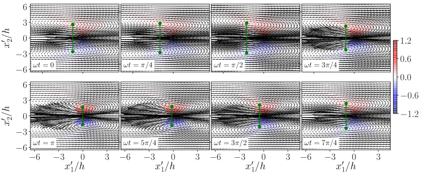
Figure 14: Vector plot of the conditionally averaged fluctuating velocity (PP case) over the $x_{3}/h=2$ wall-parallel plane. The flow has been conditioned on a local minimum streamwise velocity event in the same plane, i.e., $x_{3}=x_{3,e}$. Color contours represent the wall-normal swirling strength $\lambda_{s,3}$. Green dots identify the cores of the counter-rotating vortices.

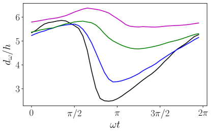
Figure 15: Spacing between the composite vortex pair cores $d_{\omega}$, corresponding to local minimum streamwise velocity events at $x_{3,e}/h=1.5$ (black lines), $x_{3,e}/h=2$ (blue lines), $x_{3,e}/h=3$ (green lines) and $x_{3,e}/h=4$ (magenta lines).

Figure 14 shows a wall-parallel slice at $x_{3}/h=2$ of the conditionally averaged fluctuating velocity field in the same plane as the triggering event. Counter-rotating vortices associated with a low-momentum region in between appear to be persistent features of the ISL throughout the pulsation cycle. Vortex cores move downstream and towards each other as $\partial\langle\overline{u}_{1}\rangle/\partial x_{3}$ increases, and the vortices intensify. This behavior occurs in the normalized time interval $\omega t\in[\pi/2,\pi]$. Instead, when $\partial\langle\overline{u}_{1}\rangle/\partial x_{3}$ decreases, the cores move upstream and further apart. Such behavior provides statistical evidence of the behavior depicted in figure 12(c,d) for the instantaneous flow field. Note that the composite counter-rotating vortex pair in the conditionally averaged flow field is in fact an ensemble average of vortex pairs in the instantaneous flow field. Thus, the spacing between the composite vortex pair cores ($d_{\omega}$) represents a suitable metric to quantify the phase-averaged widths of vortex packets in the considered flow system. Figure 15 presents $d_{\omega}$ evaluated with the triggering event at $x_{3,e}/h=\{1.5,2,3,4\}$. The trend in $d_{\omega}$ is similar to that observed in figure 8(a) for the first zero crossing of $\overline{R}_{11}$, which is an indicator of the streak width. The explanation for this behavior is that low-momentum regions are generated between the legs of the hairpins, justifying the observed linear scaling of the streak width with the cross-stream spacing of hairpin legs.

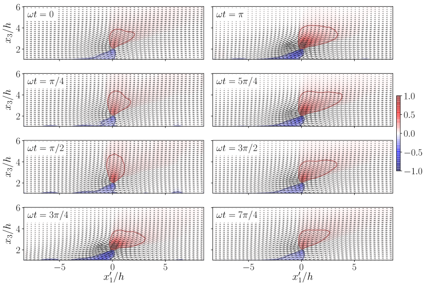
Figure 16: Time evolution of the conditionally averaged fluctuating velocity field of the PP case in the streamwise/wall-normal plane $x_{2}^{*}/h=0$ given a local minimum streamwise velocity event at $x_{3,e}/h=2$. Color contours represent the cross-stream swirling strength $\lambda_{s,2}$. Red and blue lines mark the $\lambda_{s,2}=0.1$ and $\lambda_{s,2}=-0.1$ contours, respectively.

Figure 16 and 17 depict a conditionally averaged fluctuating velocity field, which is obtained with a triggering event at $x_{3,e}/h=2$, in the $x^{\prime}_{2}=0$ plane and the $x_{1}^{\prime}=-h$ plane, respectively. Note that the $x^{\prime}_{2}=0$ plane corresponds to the center plane, and the $x_{1}^{\prime}=-h$ cross-section is located $h$ upstream of the triggering event. From Fig. 16, a region of positive $\lambda_{s,2}$ can be identified immediately above and downstream the location of the triggering event, i.e., $(x_{1}^{\prime},x_{2}^{\prime},x_{3}^{e})=(0,0,2h)$. This $\lambda_{s,2}>0$ region can be interpreted as the head of the composite hairpin vortex (Adrian et al., 2000; Ganapathisubramani et al., 2003). As $\partial\langle\overline{u}_{1}\rangle/\partial x_{3}$ increases, the vortex structure is deflected downstream and $\lambda_{s,2}$ increases, leading to enhanced upstream ejection events. This behavior is also apparent from figure 6, where the overall contribution from ejection events to $\langle\overline{u_{1}^{\prime}u_{3}^{\prime}}\rangle$ increases, while the number of ejection events reduces, highlighting enhanced individual ejection events. The deflection of the hairpin head in the downstream direction is caused by two competing factors. The first is the increase in $\langle\overline{u_{1}^{\prime}u_{3}^{\prime}}\rangle$, which leads to the downstream deflection. The second factor is the enhancement of the sweep events, which induce an upstream deflection. The first factor outweighs the second thus yielding the observed variations in the hairpin topology.

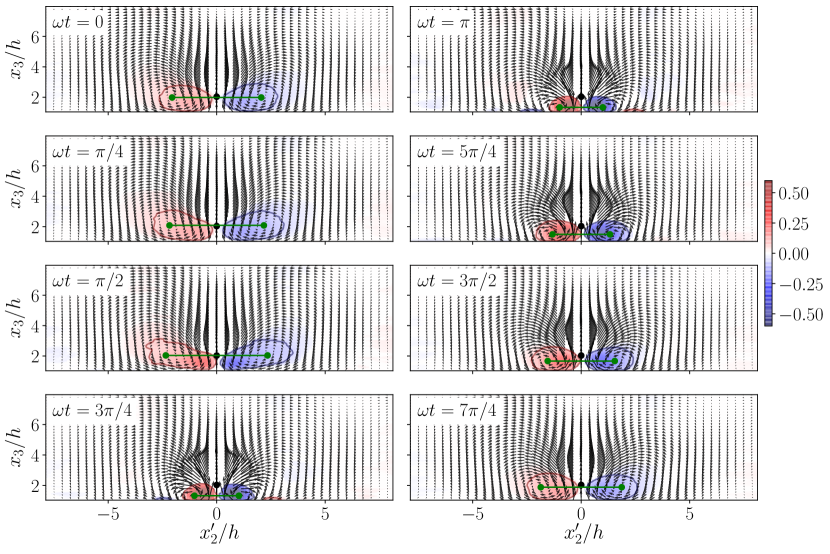
Figure 17: Time evolution of the conditionally averaged fluctuating velocity field in figure 16 in a cross-stream/wall-normal plane $x^{\prime}_{1}=-h$. Color contours represent the streamwise swirling strength $\lambda_{s,1}$. Red and blue lines mark $\lambda_{s,1}=0.1$ and $\lambda_{s,1}=-0.1$, respectively. Green dots identify the cores of the counter-rotating vortices.

Figure 17 shows the response of hairpin legs to changing $\partial\langle\overline{u}_{1}\rangle/\partial x_{3}$ in a cross-stream plane at $x_{1}^{\prime}=-h$. A pair of counter-rotating streamwise rollers is readily observed, which, as explained before, identify the legs of the composite hairpin vortex. It also further corroborates our analysis, highlighting that the spacing between the legs reduces from $\approx 5h$ at $\omega t=\pi/2$ to $\approx 2h$ at $\omega t=\pi$. This also provides a justification for findings in §3.3 and §3.4. Further, the swirling of the hairpin legs, which is quantified with $\lambda_{s,1}$ and $\lambda_{s,3}$ in the wall-normal/cross-stream and wall-parallel planes, respectively, intensifies with increasing $\partial\langle\overline{u}_{1}\rangle/\partial x_{3}$. Interestingly, when $\partial\langle\overline{u}_{1}\rangle/\partial x_{3}$ approaches its peak value at $\omega t=\pi$, a modest albeit visible secondary streamwise roller pair is induced by the hairpin legs at $x_{2}^{\prime}=\pm 3$. This suggests that the hairpin vortex not only generates new offsprings upstream and downstream, as documented in (Zhou et al., 1999; Adrian, 2007), but also in the cross-stream direction when it intensifies. The intensification of hairpin legs creates counter-rotating quasi-streamwise roller pairs between the hairpin vortices adjacent to the cross-stream direction. These roller pairs are lifted up due to the effect of the induced velocity of one roller on the other according to the Biot–Savart law, and the downstream ends of the rollers then connect, forming new hairpin structures.

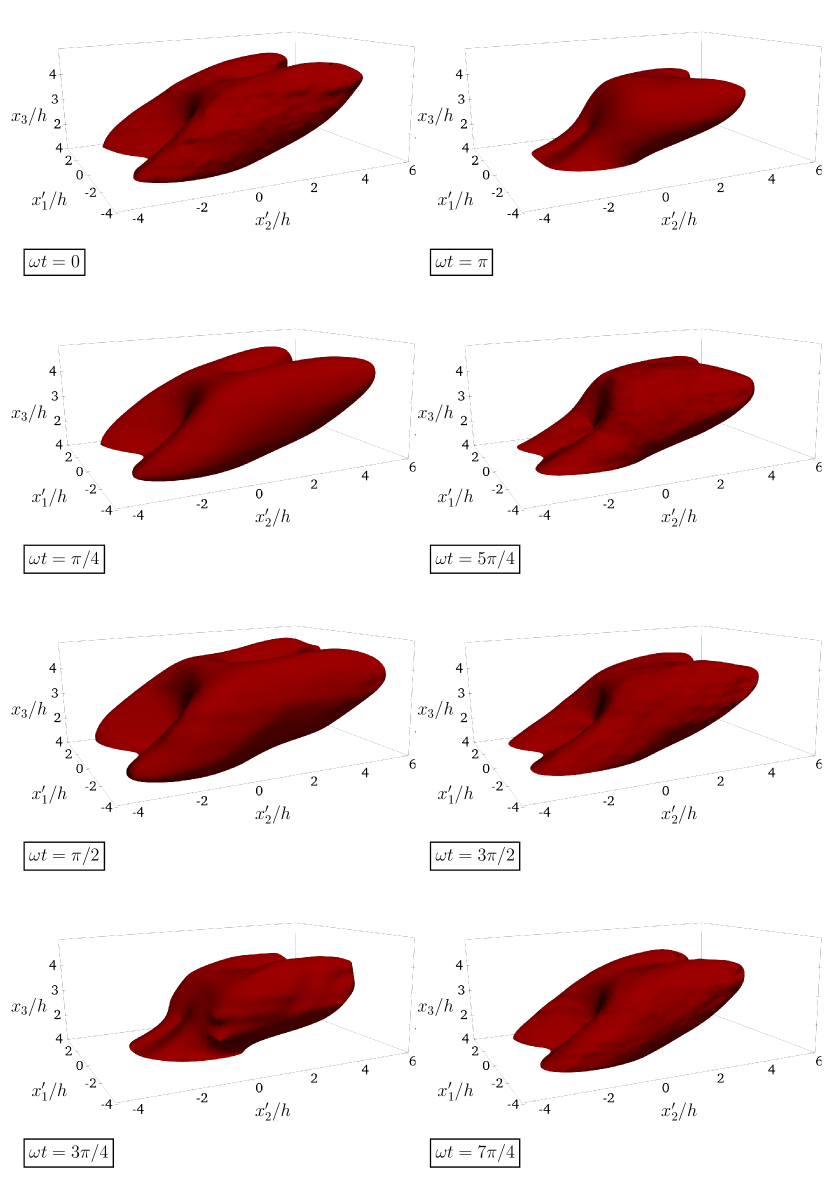
Figure 18: Time evolution of the conditionally averaged swirling field $\lambda_{s}$ of the PP case given a local minimum streamwise velocity event at $x_{3,e}=2h$. The shown iso-surfaces are for $\lambda_{s}=0.1$.

A more comprehensive picture is provided by isocontours of the conditionally averaged swirling magnitude $\lambda_{s}=0.1$ shown in figure 18. $\lambda_{s}$ is the imaginary part of the complex eigenvalue of the velocity gradient tensor (Zhou et al., 1999). In this case, the conditionally averaged swirling field corresponds to a triggering event at $x_{3,e}/h=2$. Zhou et al. (1999) pointed out that different thresholds of the iso-surface result in vortex structures of similar shapes but different sizes. $\lambda_{s}=0.1$, in this case, strikes the best compromise between descriptive capabilities and surface smoothness. Note that other vortex identification criteria, such as the Q criterion (Hunt et al., 1988) and the $\lambda_{2}$ criterion (Jeong & Hussain, 1995), are expected to result in qualitatively similar vortex structures (Chakraborty et al., 2005).

The extents of the conditional eddy in figure 18 vary substantially from roughly $10h\times 8h\times 5h$ at relatively low $\partial\langle\overline{u}_{1}\rangle/\partial x_{3}$ ($\omega t=\pi/2$), to $6h\times 6h\times 3h$ at high $\partial\langle\overline{u}_{1}\rangle/\partial x_{3}$ ($\omega t=\pi$). During the period of decreasing $\partial\langle\overline{u}_{1}\rangle/\partial x_{3}$, i.e., $0<\omega t<3\pi/4$ and $\pi<\omega t<2\pi$, the conditional eddy resembles the classic hairpin structure in the stationary case, where two hairpin legs and the hairpin head connecting the hairpin legs can be vividly observed. The sizes of the hairpin legs increase with decreasing $\partial\langle\overline{u}_{1}\rangle/\partial x_{3}$, and so does their spacing, which is in line with our prior observations based on figure 17. One possible physical interpretation for the change in the size of hairpin legs is that the reduction in swirling strength of the hairpin head resulting from a decrease in $\partial\langle\overline{u}_{1}\rangle/\partial x_{3}$ weakens the ejection between the hairpin legs, as shown in Figure 16. As a result, the swirling strength of the legs decreases, causing an increase in their size due to the conservation of angular momentum. Conversely, during the period of increasing $\partial\langle\overline{u}_{1}\rangle/\partial x_{3}$ ($3\pi/4<\omega t<\pi$), the hairpin structure is less pronounced. The conditional eddy features a strengthened hairpin head, and the intensified counter-rotating hairpin legs move closer to each other and ultimately merge into a single region of non-zero swirling strength, as apparent from Figure 18. Moreover, downstream of the conditional eddy, a pair of streamwise protrusions, known as “tongues” (Zhou et al., 1999), persist throughout the pulsatile cycle. According to Adrian (2007), these protrusions reflect the early stage of the generation process of the downstream hairpin vortex. These protrusions would eventually grow into a quasi-streamwise vortex pair and later develop a child hairpin vortex downstream of the original one.

In summary, the proposed conditional analysis complements and extends findings from §3.4 and elucidates fundamental physical mechanisms underpinning the observed variability in momentum transport (§3.2) and flow coherence (§3.3) in the considered pulsatile flow. More specifically, the analysis reveals that the time-varying shear rate resulting from the pulsatile forcing affects the topology and swirling intensity of hairpin vortices. As the shear rate increases (decreases), hairpin vortices tend to shrink (grow) with a corresponding enhancement (relaxation) of the swirling strength. These variations in hairpin geometry are responsible for the observed time-varying ejection-sweep pattern depicted in figure 6. Ejection events primarily occur between the hairpin legs, which become more widely spaced as the vortices grow and less spaced as they shrink. Therefore, a decrease in hairpin vortex size due to an increasing shear rate reduces the number of ejection events, while an increase in vortex size due to decreasing shear rate leads to an increased number of ejections. Moreover, the intensification (relaxation) of hairpin vortices at high (low) shear rates results in enhanced (attenuated) ejection events between the hairpin legs, as evidenced by figures 16 and 17. This enhancement (attenuation) of ejection events is also corroborated by results from figure 6, which indicated that high (low) shear rates decrease (increase) the number of ejection events but increase (decrease) their contribution to $\overline{u_{1}^{\prime}u_{3}^{\prime}}$. From a flow coherence perspective, this physical process also explains the observed time evolution of $\overline{R}_{11}$ (see figures 8 and 10), which is a statistical signature of hairpin packets. Changes in the size of individual hairpin vortices in response to the shear rate directly influence the dimensions of hairpin packets, as the latter are composed of multiple individual hairpin structures.

4 Conclusions

In this study, the structure of turbulence in pulsatile flow over an array of surface-mounted cuboids has been characterized and contrasted with its counterpart in a stationary flow regime. The goal is to shed light on the impact of non-stationarity on turbulence topology and its implications for momentum transfer.

The flow unsteadiness does not substantially modify the profiles of turbulent kinetic energy and resolved Reynolds shear stress in a longtime average sense, and marginally increases the height of the RSL. In terms of quadrant analysis, we have found that the flow unsteadiness does not noticeably alter the overall distribution of each quadrant. However, the ejection-sweep pattern exhibits an apparent variation during the pulsation cycle. Flow acceleration yields a large number of ejection events within the RSL, whereas flow deceleration favors sweeps. In the ISL, it is shown that the ejection-sweep pattern is mainly controlled by the intrinsic- and phase-averaged shear rate $\partial\langle\overline{u}_{1}\rangle/\partial x_{3}$ rather than by the driving pressure gradient. Specifically, the relative contribution from ejections increases, but their frequency of occurrence decreases with increasing $\partial\langle\overline{u}_{1}\rangle/\partial x_{3}$. The aforementioned time variation in the ejection-sweep pattern was later found to stem from topological variations in the structure of ISL turbulence, as deduced from inspection of the two-point streamwise velocity correlation function and the conditionally-averaged flow field.

Specifically, the geometry of hairpin vortex packets, which are the dominant coherent structures in the ISL, has been examined through the analysis of two-point velocity correlation to explore its longtime-averaged and phase-dependent characteristics. Flow unsteadiness was found to yield relatively shorter vortex packets in a longtime average sense (up to 15% discrepancy). From a phase-averaged perspective, the three-dimensional extent of hairpin packets was found to vary during the pulsation cycle and to be primarily controlled by $\partial\langle\overline{u}_{1}\rangle/\partial x_{3}$, while their tilting angle remained constant throughout. A visual examination of instantaneous structures also confirmed such behavior: the size of low-momentum regions and spacing of the hairpin legs encapsulating them were found to change with $\partial\langle\overline{u}_{1}\rangle/\partial x_{3}$, while the hairpin vortices remained aligned at a constant angle during the pulsation cycle.

Further insight into phase variations of instantaneous hairpin structures was later gained using conditional averaging operations, which provided compelling quantitative evidence for the behaviors previously observed. Specifically, the conditional averaged flow field revealed that the size and swirling intensity of the composite hairpin vortex vary considerably with $\partial\langle\overline{u}_{1}\rangle/\partial x_{3}$. When $\partial\langle\overline{u}_{1}\rangle/\partial x_{3}$ increases to its peak value, the swirling strength of the hairpin head is intensified, yielding strengthened ejections upstream of the hairpin head and a downstream deflection of the hairpin head. Following the intensification of the hairpin head, an intensification of the hairpin legs is observed, along with a narrowing of the spacing between the legs. This justifies the observed reduction in the extent of the ejection-dominated region. In other words, individual ejections become stronger and are generated at a reduced frequency as the shear rate increases, which provides a kinematic interpretation and justification for the observed time-variability of the quadrant distribution. Such a process, needless to say, is reversed when the shear rate decreases.

The findings of this study emphasize the significant influence that departures from statistically stationary flow conditions can have on the structure of ABL turbulence and associated processes. Such departures are typical in realistic ABL flows and have garnered growing attention in recent times (Mahrt & Bou-Zeid, 2020). While the study focuses on a particular type of non-stationarity, its results underscore the importance of accounting for this flow phenomenon in both geophysical and engineering applications. Flow unsteadiness-induced modifications in turbulence structure can significantly impact land- and ocean-atmosphere exchanges and the aerodynamic drag of vehicles, thus calling for dedicated efforts toward their comprehensive characterization. For example, this understanding can facilitate the development of improved non-equilibrium wall-layer models, such as those proposed in the works of Marusic et al. (2001, 2010), which utilize information on turbulence structure to enhance the predictive capabilities of wall-layer models for wall-bounded turbulence.

Declaration of Interests. The authors report no conflict of interest.

Acknowledgements. The authors acknowledge support from the Department of Civil Engineering and Engineering Mechanics at Columbia University. This material is based upon work supported by, or in part by, the Army Research Laboratory and the Army Research Office under contract/grant number W911NF-22-1-0178. This work used the Stampede2 cluster at the Texas Advanced Computing Center through allocation ATM180022 from the Extreme Science and Engineering Discovery Environment (XSEDE), which was supported by National Science Foundation grant number #1548562.

References

- Adrian (2007) Adrian, R. J. 2007 Hairpin vortex organization in wall turbulence. Phys. Fluids 19, 041301.
- Adrian et al. (2000) Adrian, R. J., Meinhart, C. D. & Tomkins, C. D. 2000 Vortex organization in the outer region of the turbulent boundary layer. J. Fluid Mech. 422, 1–54.
- Albertson & Parlange (1999a) Albertson, J. D. & Parlange, M. B. 1999a Natural integration of scalar fluxes from complex terrain. Adv. Water Resour. 23, 239–252.
- Albertson & Parlange (1999b) Albertson, J. D. & Parlange, M. B. 1999b Surface length scales and shear stress: Implications for land-atmosphere interaction over complex terrain. Water Resour. Res. 35, 2121–2132.
- Ali et al. (2017) Ali, N., Cortina, G., Hamilton, N., Calaf, M. & Cal, R. B. 2017 Turbulence characteristics of a thermally stratified wind turbine array boundary layer via proper orthogonal decomposition. J. Fluid Mech. 828, 175–195.
- Anderson et al. (2015a) Anderson, W., Barros, J. M., Christensen, K. T. & Awasthi, A. 2015a Numerical and experimental study of mechanisms responsible for turbulent secondary flows in boundary layer flows over spanwise heterogeneous roughness. J. Fluid Mech. 768, 316–347.
- Anderson et al. (2015b) Anderson, W., Li, Q. & Bou-Zeid, E. 2015b Numerical simulation of flow over urban-like topographies and evaluation of turbulence temporal attributes. J. Turbul. 16, 809–831.
- Bailey & Stoll (2016) Bailey, B. N. & Stoll, R. 2016 The creation and evolution of coherent structures in plant canopy flows and their role in turbulent transport. J. Fluid Mech. 789, 425–460.
- Balakumar & Adrian (2007) Balakumar, B. J. & Adrian, R. J. 2007 Large-and very-large-scale motions in channel and boundary-layer flows. Philos. Trans. Royal Soc. 365, 665–681.
- Bandyopadhyay (1980) Bandyopadhyay, P. 1980 Large structure with a characteristic upstream interface in turbulent boundary layers. Phys. Fluids 23, 2326–2327.
- Barros & Christensen (2014) Barros, J. M. & Christensen, K. T. 2014 Observations of turbulent secondary flows in a rough-wall boundary layer. J. Fluid Mech. 748.
- Basley et al. (2019) Basley, J., Perret, L. & Mathis, R. 2019 Structure of high reynolds number boundary layers over cube canopies. J. Fluid Mech. 870, 460–491.
- Blackwelder (1977) Blackwelder, R. 1977 On the role of phase information in conditional sampling. Phys. Fluids 20, S232–S242.
- Böhm et al. (2013) Böhm, M., Finnigan, J. J., Raupach, M. R. & Hughes, D. 2013 Turbulence structure within and above a canopy of bluff elements. Boundary-Layer Meteorol. 146, 393–419.
- Bose & Park (2018) Bose, S. T. & Park, G. I. 2018 Wall-modeled large-eddy simulation for complex turbulent flows. Annu. Rev. Fluid Mech. 50, 535–561.
- Bou-Zeid et al. (2005) Bou-Zeid, E., Meneveau, C. & Parlange, M. B. 2005 A scale-dependent lagrangian dynamic model for large eddy simulation of complex turbulent flows. Phys. Fluids 17, 025105.
- Canuto et al. (2007) Canuto, C., Hussaini, M. Y., Quarteroni, A. & Zang, T. A. 2007 Spectral methods: evolution to complex geometries and applications to fluid dynamics. Springer Science & Business Media.
- Carper & Porté-Agel (2004) Carper, M. A. & Porté-Agel, F. 2004 The role of coherent structures in subfilter-scale dissipation of turbulence measured in the atmospheric surface layer. J. Turbul. 5, 040.
- Carstensen et al. (2010) Carstensen, S., Sumer, B. M. & Fredsøe, J. 2010 Coherent structures in wave boundary layers. part 1. oscillatory motion. J. Fluid Mech. 646, 169–206.
- Carstensen et al. (2012) Carstensen, S., Sumer, B. M. & Fredsøe, J. 2012 A note on turbulent spots over a rough bed in wave boundary layers. Phys. Fluids 24, 115104.
- Castro (2007) Castro, I. P. 2007 Rough-wall boundary layers: mean flow universality. J. Fluid Mech. 585, 469–485.
- Castro et al. (2006) Castro, I. P., Cheng, H. & Reynolds, R. 2006 Turbulence over urban-type roughness: deductions from wind-tunnel measurements. Boundary-Layer Meteorol. 118, 109–131.
- Cava et al. (2017) Cava, Daniela, Mortarini, L, Giostra, Umberto, Richiardone, Renzo & Anfossi, D 2017 A wavelet analysis of low-wind-speed submeso motions in a nocturnal boundary layer. Q. J. R. Meteorol. Soc. 143, 661–669.
- Chakraborty et al. (2005) Chakraborty, P., Balachandar, S. & Adrian, R. J. 2005 On the relationships between local vortex identification schemes. J. Fluid Mech. 535, 189–214.
- Chauhan et al. (2013) Chauhan, K., Hutchins, N., Monty, J. & Marusic, I. 2013 Structure inclination angles in the convective atmospheric surface layer. Boundary-Layer Meteorol. 147, 41–50.
- Chester et al. (2007) Chester, S., Meneveau, C. & Parlange, M. B. 2007 Modeling turbulent flow over fractal trees with renormalized numerical simulation. J. Comput. Phys. 225, 427–448.
- Christen et al. (2007) Christen, A., van Gorsel, E. & Vogt, R. 2007 Coherent structures in urban roughness sublayer turbulence. Intl J. Climatol. 27, 1955–1968.
- Christensen & Adrian (2001) Christensen, K. T. & Adrian, R. J. 2001 Statistical evidence of hairpin vortex packets in wall turbulence. J. Fluid Mech. 431, 433–443.
- Coceal et al. (2007) Coceal, O., Dobre, A., Thomas, T. G. & Belcher, S. E. 2007 Structure of turbulent flow over regular arrays of cubical roughness. J. Fluid Mech. 589, 375–409.
- Costamagna et al. (2003) Costamagna, P., Vittori, G. & Blondeaux, P. 2003 Coherent structures in oscillatory boundary layers. J. Fluid Mech. 474, 1–33.
- Dennis & Nickels (2011) Dennis, D. J. C. & Nickels, T. B. 2011 Experimental measurement of large-scale three-dimensional structures in a turbulent boundary layer. part 1. vortex packets. J. Fluid Mech. 673, 180–217.
- Dong et al. (2020) Dong, S., Huang, y., Yuan, X. & Lozano-Durán, A. 2020 The coherent structure of the kinetic energy transfer in shear turbulence. J. Fluid Mech. 892, A22.
- Dupont & Brunet (2008) Dupont, S. & Brunet, Y. 2008 Influence of foliar density profile on canopy flow: a large-eddy simulation study. Agric. For. Meteorol. 148, 976–990.
- Dupont & Patton (2012) Dupont, S. & Patton, E. G. 2012 Influence of stability and seasonal canopy changes on micrometeorology within and above an orchard canopy: The chats experiment. Agric. For. Meteorol. 157, 11–29.
- Eitel-Amor et al. (2015) Eitel-Amor, G., Örlü, R., Schlatter, P. & Flores, O. 2015 Hairpin vortices in turbulent boundary layers. Phys. Fluids 27 (2), 025108.
- Elsinga et al. (2012) Elsinga, G. E., Poelma, C., Schröder, A., Geisler, R., Scarano, F. & Westerweel, J. 2012 Tracking of vortices in a turbulent boundary layer. J. Fluid Mech. 697, 273–295.
- Fernando (2010) Fernando, H. J. S. 2010 Fluid dynamics of urban atmospheres in complex terrain. Annu. Rev. Fluid Mech. 42, 365–389.
- Finnigan (2000) Finnigan, J. J. 2000 Turbulence in plant canopies. Annu. Rev. Fluid Mech. 32, 519–571.
- Finnigan et al. (2009) Finnigan, J. J., Shaw, R. H. & Patton, E. G. 2009 Turbulence structure above a vegetation canopy. J. Fluid Mech. 637, 387–424.
- Ganapathisubramani et al. (2003) Ganapathisubramani, B., Longmire, E. K. & Marusic, I 2003 Characteristics of vortex packets in turbulent boundary layers. J. Fluid Mech. 478, 35–46.
- Gavrilov et al. (2013) Gavrilov, K., Morvan, D., Accary, G., Lyubimov, D. & Meradji, S. 2013 Numerical simulation of coherent turbulent structures and of passive scalar dispersion in a canopy sub-layer. Comput. Fluids 78, 54–62.
- Giometto et al. (2016) Giometto, M. G., Christen, A., Meneveau, C., Fang, J., Krafczyk, M. & Parlange, M. B. 2016 Spatial characteristics of roughness sublayer mean flow and turbulence over a realistic urban surface. Boundary-Layer Meteorol. 160, 425–452.
- Grimsdell & Angevine (2002) Grimsdell, A. W. & Angevine, W. M. 2002 Observations of the afternoon transition of the convective boundary layer. J. Appl. Meteorol. Climatol. 41, 3–11.
- Guala et al. (2012) Guala, M., Tomkins, C. D., Christensen, K. T. & Adrian, R. J. 2012 Vortex organization in a turbulent boundary layer overlying sparse roughness elements. J. Hydraul. Res. 50, 465–481.
- Head & Bandyopadhyay (1981) Head, M. R. & Bandyopadhyay, P. 1981 New aspects of turbulent boundary-layer structure. J. Fluid Mech. 107, 297–338.
- Hicks et al. (2018) Hicks, B. B., Pendergrass, W. R., Baker, B. D., Saylor, R. D., O’Dell, D. L., Eash, N. S. & McQueen, J. T. 2018 On the relevance of . Boundary-Layer Meteorol. 167, 285–301.
- Hommema & Adrian (2003) Hommema, S. E. & Adrian, R. J. 2003 Packet structure of surface eddies in the atmospheric boundary layer. Boundary-Layer Meteorol. 106, 147–170.
- Hoover et al. (2015) Hoover, J. D., Stauffer, D. R., Richardson, S. J., Mahrt, L., Gaudet, B. J. & Suarez, A. 2015 Submeso motions within the stable boundary layer and their relationships to local indicators and synoptic regime in moderately complex terrain. J. Appl. Meteorol. and Climatol. 54, 352–369.
- Hu et al. (2023) Hu, R., Dong, S. & Vinuesa, R. 2023 General attached eddies: Scaling laws and cascade self-similarity. Phys. Rev. Fluids 8, 044603.
- Huang et al. (2009) Huang, J., Cassiani, M. & Albertson, J. D. 2009 Analysis of coherent structures within the atmospheric boundary layer. Boundary-Layer Meteorol. 131, 147–171.
- Hunt et al. (1988) Hunt, J. C. R., Wray, A. A. & Moin, P. 1988 Eddies, streams, and convergence zones in turbulent flows. Studying Turbulence Using Numerical Simulation Databases, 2. Proceedings of the 1988 Summer Program .
- Huq et al. (2007) Huq, P., White, L. A., Carrillo, A., Redondo, J., Dharmavaram, S. & Hanna, S. R. 2007 The shear layer above and in urban canopies. J. Appl. Meteorol. Climatol. 46, 368–376.
- Hutchins et al. (2012) Hutchins, N., Chauhan, K., Marusic, I., Monty, J. & Klewicki, J. 2012 Towards reconciling the large-scale structure of turbulent boundary layers in the atmosphere and laboratory. Boundary-Layer Meteorol. 145, 273–306.
- Jeong & Hussain (1995) Jeong, J. & Hussain, F. 1995 On the identification of a vortex. J. Fluid Mech. 285, 69–94.
- Kanda et al. (2004) Kanda, M., Moriwaki, R. & Kasamatsu, F. 2004 Large-eddy simulation of turbulent organized structures within and above explicitly resolved cube arrays. Boundary-Layer Meteorol. 112, 343–368.
- Katul et al. (2006) Katul, G., Poggi, D., Cava, D. & Finnigan, J. 2006 The relative importance of ejections and sweeps to momentum transfer in the atmospheric boundary layer. Boundary-Layer Meteorol. 120, 367–375.
- Kim & Moin (1985) Kim, J. & Moin, P. 1985 Application of a fractional-step method to incompressible navier-stokes equations. J. Comput. Phys. 59, 308–323.
- Kim & Moin (1986) Kim, J. & Moin, P. 1986 The structure of the vorticity field in turbulent channel flow. part 2. study of ensemble-averaged fields. J. Fluid Mech. 162, 339–363.
- Klewicki et al. (2014) Klewicki, J., Philip, J., Marusic, I., Chauhan, K. & Morrill-Winter, C. 2014 Self-similarity in the inertial region of wall turbulence. Phys. Rev. E 90, 063015.
- Krogstad & Antonia (1994) Krogstad, P. Å. & Antonia, R. A. 1994 Structure of turbulent boundary layers on smooth and rough walls. J. Fluid Mech. 277, 1–21.
- Lee et al. (2011) Lee, J. H., Sung, H. J. & Krogstad, P. 2011 Direct numerical simulation of the turbulent boundary layer over a cube-roughened wall. J. Fluid Mech. 669, 397–431.
- Leonardi & Castro (2010) Leonardi, S. & Castro, I. P. 2010 Channel flow over large cube roughness: a direct numerical simulation study. J. Fluid Mech. 651, 519–539.
- Li & Bou-Zeid (2011) Li, D. & Bou-Zeid, E. 2011 Coherent structures and the dissimilarity of turbulent transport of momentum and scalars in the unstable atmospheric surface layer. Boundary-Layer Meteorol. 140, 243–262.
- Li & Bou-Zeid (2019) Li, Q. & Bou-Zeid, E. 2019 Contrasts between momentum and scalar transport over very rough surfaces. J. Fluid Mech. 880, 32–58.
- Li & Giometto (2022) Li, W. & Giometto, M. G. 2022 Mean flow and turbulence in unsteady canopy layers. Under review for J. Fluid Mech. .
- Lohou et al. (2000) Lohou, F., Druilhet, A., Campistron, B., Redelsperger, J. L. & Saïd, F. 2000 Numerical study of the impact of coherent structures on vertical transfers in the atmospheric boundary layer. Boundary-Layer Meteorol. 97, 361–383.
- Lozano-durán et al. (2020) Lozano-durán, A., Giometto, M. G., Park, G. I. & Moin, P. 2020 Non-equilibrium three-dimensional boundary layers at moderate Reynolds numbers. J. Fluid Mech. 883, A20–1.
- Mahrt (2007) Mahrt, L. 2007 The influence of nonstationarity on the turbulent flux–gradient relationship for stable stratification. Boundary-Layer Meteorol. 125, 245–264.
- Mahrt (2008) Mahrt, L. 2008 The influence of transient flow distortion on turbulence in stable weak-wind conditions. Boundary-Layer Meteorol. 127, 1–16.
- Mahrt (2009) Mahrt, L. 2009 Characteristics of submeso winds in the stable boundary layer. Boundary-Layer Meteorol. 130, 1–14.
- Mahrt (2014) Mahrt, L. 2014 Stably stratified atmospheric boundary layers. Annu. Rev. Fluid Mech. 46, 23–45.
- Mahrt & Bou-Zeid (2020) Mahrt, L. & Bou-Zeid, E. 2020 Non-stationary boundary layers. Boundary-Layer Meteorol. 177, 189–204.
- Mahrt et al. (2013) Mahrt, L., Thomas, C., Richardson, S., Seaman, N., Stauffer, D. & Zeeman, M. 2013 Non-stationary generation of weak turbulence for very stable and weak-wind conditions. Boundary-Layer Meteorol. 147, 179–199.
- Margairaz et al. (2018) Margairaz, F., Giometto, M. G., Parlange, M. B. & Calaf, M. 2018 Comparison of dealiasing schemes in large-eddy simulation of neutrally stratified atmospheric flows. Geosci. Model Dev. 11, 4069–4084.
- Marusic et al. (2001) Marusic, I, Kunkel, G. J. & Porté-Agel, F. 2001 Experimental study of wall boundary conditions for large-eddy simulation. J. Fluid Mech. 446, 309–320.
- Marusic et al. (2010) Marusic, I., Mathis, R. & Hutchins, N. 2010 Predictive model for wall-bounded turbulent flow. Science 329, 193–196.
- Marusic & Monty (2019) Marusic, I. & Monty, J. P. 2019 Attached eddy model of wall turbulence. Annu. Rev. Fluid Mech. 51, 49–74.
- Marusic et al. (2013) Marusic, I., Monty, J. P., Hultmark, M. & Smits, A. J. 2013 On the logarithmic region in wall turbulence. J. Fluid Mech. 716, R3.
- Mazzuoli & Vittori (2019) Mazzuoli, M. & Vittori, G. 2019 Turbulent spots in an oscillatory flow over a rough wall. Eur. J. Mech. B/Fluids 78, 161–168.
- Meneveau & Marusic (2013) Meneveau, C. & Marusic, I. 2013 Generalized logarithmic law for high-order moments in turbulent boundary layers. J. Fluid Mech. 719, R1.
- Michioka et al. (2014) Michioka, T., Takimoto, H. & Sato, A. 2014 Large-eddy simulation of pollutant removal from a three-dimensional street canyon. Boundary-Layer Meteorol. 150, 259–275.
- Mittal & Iaccarino (2005) Mittal, R. & Iaccarino, G. 2005 Immersed boundary methods. Annu. Rev. Fluid Mech. 37, 239–261.
- Moin & Kim (1982) Moin, P. & Kim, J. 1982 Numerical investigation of turbulent channel flow. J. Fluid Mech. 118, 341–377.
- Moin & Kim (1985) Moin, P. & Kim, J. 1985 The structure of the vorticity field in turbulent channel flow. part 1. analysis of instantaneous fields and statistical correlations. J. Fluid Mech. 155, 441–464.
- Monti et al. (2002) Monti, P., Fernando, H. J. S., Princevac, M., Chan, W. C., Kowalewski, T. A. & Pardyjak, E. R. 2002 Observations of flow and turbulence in the nocturnal boundary layer over a slope. J. Atmos. Sci. 59, 2513–2534.
- Morris et al. (2007) Morris, S. C., Stolpa, S. R., Slaboch, P. E. & Klewicki, J. C. 2007 Near-surface particle image velocimetry measurements in a transitionally rough-wall atmospheric boundary layer. J. Fluid Mech. 580, 319–338.
- Novak et al. (2000) Novak, M. D., Warland, J. S., Orchansky, A. L., Ketler, R. & Green, S. 2000 Wind tunnel and field measurements of turbulent flow in forests. part i: Uniformly thinned stands. Boundary-Layer Meteorol. 95, 457–495.
- Oke et al. (2017) Oke, T. R., Mills, G., Christen, A. & Voogt, J. A. 2017 Urban climates. Cambridge University Press, In Press.
- Orszag (1970) Orszag, S. A. 1970 Analytical theories of turbulence. J. Fluid Mech. 41, 363–386.
- Orszag & Pao (1975) Orszag, S. A. & Pao, Y. 1975 Numerical computation of turbulent shear flows. In Adv. Geophys., , vol. 18, pp. 225–236. Elsevier.
- Pan et al. (2014) Pan, Y., Chamecki, M. & Isard, S. A. 2014 Large-eddy simulation of turbulence and particle dispersion inside the canopy roughness sublayer. J. Fluid Mech. 753, 499–534.
- Perry & Chong (1982) Perry, A. E. & Chong, M. S. 1982 On the mechanism of wall turbulence. J. Fluid Mech. 119, 173–217.
- Piomelli (2008) Piomelli, U. 2008 Wall-layer models for large-eddy simulations. Prog. Aerosp. Sci. 44, 437–446.
- Pokrajac et al. (2007) Pokrajac, D., Campbell, L. J., Nikora, V., Manes, C. & McEwan, I. 2007 Quadrant analysis of persistent spatial velocity perturbations over square-bar roughness. Exp. Fluids 42, 413–423.
- Raupach et al. (1986) Raupach, M. R., Coppin, P. A. & Legg, B. J. 1986 Experiments on scalar dispersion within a model plant canopy part i: The turbulence structure. Boundary-Layer Meteorol. 35, 21–52.
- Raupach et al. (1996) Raupach, M. R., Finnigan, J. J. & Brunet, Y. 1996 Coherent eddies and turbulence in vegetation canopies: the mixing-layer analogy. In Boundary-Layer Meteorol., pp. 351–382. Springer.
- Reynolds & Castro (2008) Reynolds, R. T. & Castro, I. P. 2008 Measurements in an urban-type boundary layer. Exp. Fluids 45, 141–156.
- Salesky & Anderson (2020) Salesky, S. T. & Anderson, W. 2020 Revisiting inclination of large-scale motions in unstably stratified channel flow. J. Fluid Mech. 884.
- Salon et al. (2007) Salon, S., Armenio, V. & Crise, A. 2007 A numerical investigation of the stokes boundary layer in the turbulent regime. J. Fluid Mech. 570, 253–296.
- Schmid et al. (2019) Schmid, M. F., Lawrence, G. A., Parlange, M. B. & Giometto, M. G. 2019 Volume averaging for urban canopies. Boundary-Layer Meteorol. 173, 349–372.
- Scotti & Piomelli (2001) Scotti, A. & Piomelli, U. 2001 Numerical simulation of pulsating turbulent channel flow. Phys. Fluids 13, 1367–1384.
- Smith et al. (1991) Smith, C. R. T., Walker, J. D. A., Haidari, A. H. & Sobrun, U. 1991 On the dynamics of near-wall turbulence. Philos. Trans. R. Soc. London, Ser. A 336, 131–175.
- Smits et al. (2011) Smits, A. J., McKeon, B. J. & Marusic, I. 2011 High–reynolds number wall turbulence. Annu. Rev. Fluid Mech. 43, 353–375.
- Squire et al. (2017) Squire, D. T., Hutchins, N., Morrill-Winter, C., Schultz, M. P., Klewicki, J. C. & Marusic, I. 2017 Applicability of taylor’s hypothesis in rough-and smooth-wall boundary layers. J. Fluid Mech. 812, 398–417.
- Stanislas et al. (2008) Stanislas, M., Perret, L. & Foucaut, J. 2008 Vortical structures in the turbulent boundary layer: a possible route to a universal representation. J. Fluid Mech. 602, 327–382.
- Stull (1988) Stull, R. B. 1988 An introduction to boundary layer meteorology, , vol. 13. Springer Science & Business Media.
- Takimoto et al. (2013) Takimoto, H., Inagaki, A., Kanda, M., Sato, A. & Michioka, T. 2013 Length-scale similarity of turbulent organized structures over surfaces with different roughness types. Boundary-Layer Meteorol. 147, 217–236.
- Theodorsen (1952) Theodorsen, T. 1952 Mechanisms of turbulence. In Proceedings of the 2^¡ nd¿ Midwestern Conference on Fluid Mechanics, 1952.
- Tomkins & Adrian (2003) Tomkins, C. D. & Adrian, R. J. 2003 Spanwise structure and scale growth in turbulent boundary layers. J. Fluid Mech. 490, 37–74.
- Townsend (1976) Townsend, A. A. 1976 The structure of turbulent shear flow. Cambridge university press.
- Tseng et al. (2006) Tseng, Y. H., Meneveau, C. & Parlange, M. B. 2006 Modeling flow around bluff bodies and predicting urban dispersion using large eddy simulation. Environ. Sci. Technol. 40, 2653–2662.
- Volino et al. (2007) Volino, R. J., Schultz, M. P. & Flack, K. A. 2007 Turbulence structure in rough-and smooth-wall boundary layers. J. Fluid Mech. 592, 263–293.
- Volino et al. (2011) Volino, R. J., Schultz, M. P. & Flack, K. A. 2011 Turbulence structure in boundary layers over periodic two-and three-dimensional roughness. J. Fluid Mech. 676, 172–190.
- Wallace (2016) Wallace, J. M. 2016 Quadrant analysis in turbulence research: history and evolution. Annu. Rev. Fluid Mech. 48, 131–158.
- Wallace et al. (1972) Wallace, J. M., Eckelmann, H. & Brodkey, R. S. 1972 The wall region in turbulent shear flow. J. Fluid Mech. 54, 39–48.
- Wang et al. (2014) Wang, L., Li, D., Gao, Z., Sun, T., Guo, X. & Bou-Zeid, E. 2014 Turbulent transport of momentum and scalars above an urban canopy. Boundary-Layer Meteorol. 150, 485–511.
- Watanabe (2004) Watanabe, T. 2004 Large-eddy simulation of coherent turbulence structures associated with scalar ramps over plant canopies. Boundary-Layer Meteorol. 112, 307–341.
- Wu & Christensen (2007) Wu, Y. & Christensen, K. T. 2007 Outer-layer similarity in the presence of a practical rough-wall topography. Phys. Fluids 19, 085108.
- Xie et al. (2008) Xie, Z., Coceal, O. & Castro, I. P. 2008 Large-eddy simulation of flows over random urban-like obstacles. Boundary-Layer Meteorol. 129, 1–23.
- Yang et al. (2016) Yang, X. I. A., Marusic, I. & Meneveau, C. 2016 Moment generating functions and scaling laws in the inertial layer of turbulent wall-bounded flows. J. Fluid Mech. 791, R2.
- Yang & Meneveau (2016) Yang, X. I. A. & Meneveau, C. 2016 Recycling inflow method for simulations of spatially evolving turbulent boundary layers over rough surfaces. J. Turbul. 17, 75–93.
- Zhang et al. (2022) Zhang, W., Zhu, X., Yang, X. I. A. & Wan, M. 2022 Evidence for raupach et al.’s mixing-layer analogy in deep homogeneous urban-canopy flows. J. Fluid Mech. 944, A46.
- Zhang & Simons (2019) Zhang, X. & Simons, R. 2019 Experimental investigation on the structure of turbulence in the bottom wave-current boundary layers. Coast. Eng. 152, 103511.
- Zhou et al. (1999) Zhou, J., Adrian, R. J., Balachandar, S. & Kendall, T. 1999 Mechanisms for generating coherent packets of hairpin vortices in channel flow. J. Fluid Mech. 387, 353–396.