Choosing the Right Approach at the Right Time: A Comparative Analysis of Causal Effect Estimation using Confounder Adjustment and Instrumental Variables

Abstract

In observational studies, unobserved confounding is a major barrier in isolating the average causal effect (ACE). In these scenarios, two main approaches are often used: confounder adjustment for causality (CAC) and instrumental variable analysis for causation (IVAC). Nevertheless, both are subject to untestable assumptions and, therefore, it may be unclear which assumption violation scenarios one method is superior in terms of mitigating inconsistency for the ACE. Although general guidelines exist, direct theoretical comparisons of the trade-offs between CAC and the IVAC assumptions are limited. Using ordinary least squares (OLS) for CAC and two-stage least squares (2SLS) for IVAC, we analytically compare the relative inconsistency for the ACE of each approach under a variety of assumption violation scenarios and discuss rules of thumb for practice. Additionally, a sensitivity framework is proposed to guide analysts in determining which approach may result in less inconsistency for estimating the ACE with a given dataset. We demonstrate our findings both through simulation and an application examining whether maternal stress during pregnancy affects a neonate’s birthweight. The implications of our findings for causal inference practice are discussed, providing guidance for analysts for judging whether CAC or IVAC may be more appropriate for a given situation.

1 Introduction

A common goal in observational studies is to estimate the average causal effect (ACE) of a treatment or exposure on a specific outcome such as the effect of maternal stress during pregnancy on a child’s birthweight. Due to the exposure not being randomized, the presence of confounders may bias estimates of the ACE. Confounders are factors that influence both the level of exposure (or treatment assignment) and the outcome. If uncontrolled for, confounders can create extraneous differences between the exposure groups that make it difficult to isolate the causal effect. The effectiveness of confounder adjustment for causality (CAC), however, is contingent on the untestable assumption that all possible confounders, or suitable proxies, are present in the dataset and have been accounted for appropriately. In other words, we cannot use observed data to prove that the CAC is consistent for the ACE. A simple example is if a mother’s obstetric risk, a known confounder for stress and birthweight, and any proxies were missing from the dataset we would like to analyze. Without a priori knowledge that obstetric risk was a confounder, we would not be able to ascertain that the CAC assumptions were violated.

An alternative approach that may avoid concerns about unobserved confounders is the instrumental variable (IV) approach, or instrumental variable analysis for causation (IVAC). An IV is defined by three main conditions: (i) it influences the treatment assignment (relevance), (ii) it is not a cause of the outcome after conditioning on treatment assignment (exclusion restriction), and (iii) it is not associated with unobserved confounders (independence). In the event that we have a variable that satisfies these conditions, we could then use variation in the IV as a proxy for variation in the treatment and measure the effect on the outcome. Importantly, by (iii), the variation in the IV is independent from unobserved confounding and, therefore, unlike CAC, IVAC does not require appropriately accounting for all possible confounding to consistently estimate the ACE.[1]

When choosing to use CAC over the IVAC, and vice-versa, we trade one set of untestable assumptions for another. For CAC, we cannot prove that we have accounted for all confounders while, for IVAC, we cannot prove we have a valid IV. For example, proving the exclusion restriction requires us to establish the lack of a direct relationship between the IV and outcome, or a null result, which is not possible with data. Furthermore, to be consistent for the ACE, the IVAC must meet certain untestable conditions surrounding treatment effect heterogeneity. We therefore have no guarantee that under either approach our produced estimate is consistent for the ACE. Despite this, we remain interested in estimating the ACE and subsequently direct our efforts towards attempting to estimate a parameter with the least possible distance from the ACE. In this vein, the key question and central premise of the current manuscript focuses on addressing the following question in practice: under the potential violation of the untestable assumptions, when is the parameter estimated by CAC closer to the ACE than that of IVAC, and vice versa?

In the literature, there exist general guidelines surrounding whether CAC is more appropriate than IVAC.[1, 2] Generally, we contend that analysts should weigh whether the potential degree of unobserved confounding outweighs the potential for violations in the IV assumptions. There is, however, little by way of theoretical research that directly compares the two approaches to assess these trade-offs. Focusing on ordinary least squares (OLS) for CAC and two-stage least squares (2SLS) for IVAC, there are two overarching goals we seek to accomplish with this paper. Firstly, we seek to analytically compare the inconsistency of 2SLS to OLS in a variety of scenarios involving assumption violations. Next, we provide a sensitivity framework to guide analysts in determining whether the inconsistency of 2SLS is more than that of OLS, and vice versa.

In order to more succinctly express the relative performance of OLS and 2SLS under assumption violations, we focus on the scenario where, for a given variable, we must decide on whether the variable should be adjusted for as a confounder in OLS, used as an IV in 2SLS, or not incorporated into the analysis at all. Note that we allow confounders to be adjusted for in 2SLS – an IV is only used in the first stage whereas confounders would need to be present in both the first and second stage.

To our knowledge, there is no existing theoretical literature directly comparing the trade-offs of pursuing CAC versus IVAC, though authors have considered the impact of assumption violations in both settings. The first area of literature relevant to the themes of our paper is bias amplification, which refers to the fact that using certain variables as confounders may increase pre-existing bias due to unobserved confounding. In the linear setting, an IV is a bias amplifier.[3, 4, 5, 6] In these papers, the authors compare the consistency for the ACE with and without adjusting for an IV. Pearl (2012) provides an extension where there is an imperfect IV (in that the exclusion restriction is violated) and shows that under certain conditions, adjusting for the imperfect IV may actually reduce bias. Nevertheless, he does not address whether this variable may be more appropriately used in 2SLS.

The bias amplification literature and, by extension, our findings have important implications on applied practice. In particular, the rise of data-driven variable selection approaches for the propensity score, or probability of receiving the intervention, in confounder methods and first-stage for IV analysis. Though IVs, by definition, influence the treatment assignment, they may amplify bias if included in the model for the propensity score.[3] For IV methods, though a variable may not be a perfect IV it may still be worth using it as such. In addition, data-driven modeling of the first-stage may, for example, shrink to zero an important confounder used to achieve the IV assumptions. The gain in the strength of the first-stage may, however, offset the penalty incurred by omitted variable bias in 2SLS. As it stands, these intuitions are difficult to incorporate into variable selection procedures. With this work, we seek to elucidate these complicated scenarios.

In another area of the literature, there has been some work related to comparing OLS to 2SLS under the violation of IV assumptions. It is a well-known result that if an IV is poorly predictive of the intervention (i.e. weak), then small violations in the exclusion restriction and independence assumption can lead to large inconsistencies for the IV estimand.[7, 8]. In addition, to assess the independence assumption, one may compare the impact of intentionally omitting an observed confounder on OLS and 2SLS in order to compare the sensitivity of OLS to that of 2SLS in estimating the ACE.[9] The main assumption behind this procedure is that the impact of omitting an observed confounder on the consistency of OLS and 2SLS is similar to that of omitting a correlated unobserved confounder. A similar assumption and "benchmarking" procedure will be used in our sensitivity analysis.

There are several procedures in the literature regarding sensitivity analyses for violations in IV assumptions. For example, Cinelli and Hazlett (2022) provide a compelling framework and visualization scheme for omitted variable bias in 2SLS based on several partial $R^{2}$ measures.[10] Their framework addresses the question of how large the impact of an unobserved confounder would have to be in order to qualitatively change the inferential conclusions of a study, which covers both violations of the exclusion restriction and independence assumptions. A similar procedure to this is the E-value.[11] While we use many of the same tools – notably benchmarking unobserved $R^{2}$ measures with observed data from Cinelli and Hazlett (2022) – we do not focus on this sensitivity analysis paradigm of hypothesis testing but instead consider the relative inconsistencies of CAC and IVAC for the ACE.

Another complication to IVAC lies in treatment effect heterogeneity. In this setting, Imbens and Angrist (1994) state that, under monotonicity conditions, IVAC identifies the local average causal effect (LACE) or the causal effect of the "compliers" subpopulation (those whose treatment assignment varies with the IV).[12] If the factors that determine compliance also cause treatment effect heterogeneity, then the LACE may not be equal to the ACE. Hartwig et al. (2020) and Wang and Tchetgen Tchetgen (2018) give clear explanations of the assumptions needed for the LACE to equal the ACE.[13, 14] Essentially, the heterogeneity between the treatment and outcome should be independent of both the IV and the effect modification between the treatment and outcome. For the ease of parameterization in our paper, we will use Wang and Tchetgen Tchetgen’s notion that one of two conditions must be met: (i) no unmeasured confounders are additive effect modifiers of the relationship of both the instrument and treatment or (ii) no unmeasured confounders are additive effect modifiers the treatment and the outcome.

The rest of the paper is organized as follows. First, we provide the general model setting of interest and introduce relative notation. We then present results regarding the consistency of no adjustment, OLS, and 2SLS for the scenarios of an exclusion restriction violation, independence violation, and treatment effect heterogeneity relevant to IV estimation with and without covariates. In all scenarios, we consider unobserved confounding and isolate the impact of individual assumption violations (e.g. both an exclusion restriction and independence violation). Following this, we present a sensitivity analysis procedure based on partial $R^{2}$ and benchmarking unobserved quantities with observed quantities. The goal of this procedure is to give the analyst relevant information to assess the plausibility of whether it may be more appropriate to adjust for a variable in OLS or 2SLS. Next, in simulations, we verify our closed-form results and demonstrate the use of the sensitivity analysis procedure in a variety of scenarios. Then, we apply the procedure to a real world dataset studying a neonate’s birthweight as a function of maternal stress during pregnancy. We conclude with a discussion regarding the implications of our closed form results on the practice of causal inference and, additionally, provide further guidance on how to use our sensitivity analysis procedure.

2 Notation and Set-Up

Our goal is to estimate the ACE of some continuous treatment $X$ on an outcome $Y$, denoted as $\beta_{1}=\frac{\partial}{\partial x}E[Y|do(x)]$ in Pearl’s notation.[15] We depict the causal relationships in Figure 1, a directed acyclic graph (DAG) with edge weights $c_{0},\dots,c_{3}$. We further consider the following structural equations where $E[\epsilon_{1}|U,Z]=0$ and $E[\epsilon_{2}|X,U]=0$:

$$X=\alpha_{1}U+\alpha_{2}Z+\epsilon_{1},$$ (1)

$$Y=\beta_{1}X+\beta_{2}U+\epsilon_{2}.$$ (2)

Figure 1: A directed acyclic graph with one confounder and one instrumental variable.

Given that all variables in Figure (1) are standardized to have mean $0$ and variance $1$, the edge weights are equivalent to the coefficients in Eqs. (1) and (2). For example, the ACE, $\beta_{1}$, is the same as the edge weight $c_{0}$. In addition, $\alpha_{1}=c_{1}$, $\alpha_{2}=c_{3}$, $\beta_{1}=c_{0}$, and $\beta_{2}=c_{2}$. This equivalence will be helpful in visually expressing assumptions surrounding different scenarios. Furthermore, the edge weights are correlations and are bounded between $-1$ and $1$.

Throughout, we assume the stable unit treatment value assumption (SUTVA) of consistency and no interference. Because $U$ is unobserved, we must estimate the the following reduced form regression where the subscript $R$ indicates these are the values related to the reduced regression

$$Y=\beta_{1}^{R}X+\epsilon_{2}^{R}.$$ (3)

$U$ is a confounder because it both influences $X$ and $Y$, and, therefore, because we have failed to block the path through $U$, $\hat{\beta}_{1}^{R}$ is inconsistent for the ACE. Alternatively, to estimate the ACE, we may utilize $Z$, which is a valid IV if

1. $\alpha_{2}>0$ (relevance)

2. $Z$ is not a cause of $Y$ conditional on $X$ (exclusion restriction)

3. $Z$ is not influenced by any unaccounted for confounders such that $Z\mathchoice{\mathrel{\hbox to0.0pt{\kern 7.63889pt\kern-5.27776pt$\displaystyle\not$\hss}{\perp\mkern-9.5mu\perp}}}{\mathrel{\hbox to0.0pt{\kern 7.63889pt\kern-5.27776pt$\textstyle\not$\hss}{\perp\mkern-9.5mu\perp}}}{\mathrel{\hbox to0.0pt{\kern 2.61118pt\kern-4.11108pt$\scriptstyle\not$\hss}{\perp\mkern-9.5mu\perp}}}{\mathrel{\hbox to0.0pt{\kern 1.11118pt\kern-3.3333pt$\scriptscriptstyle\not$\hss}{\perp\mkern-9.5mu\perp}}}Y|X$ (independence).

Supposing that there is no treatment effect heterogeneity or that the conditions of Hartwig et al. (2020) or Wang and Tchetgen Tchetgen (2018) [13, 14] are met, we have $\beta_{IV}=\frac{Cov(Z,Y)}{Cov(X,Z)}=\frac{\beta_{1}\alpha_{1}}{\alpha_{1}}=\beta_{1}$, and hence 2SLS will provide a consistent estimate of the ACE.

We are interested in estimating and comparing the following estimands: the causal effect i.e. Eq. (4), one that omits $Z$ i.e. Eq. (5), one that uses $Z$ as a confounder i.e. Eq. (6), and one that utilizes $Z$ as an IV i.e. Eq.(7):

$$A_{1}=\frac{\partial}{\partial x}E[Y|do(x)]=c_{0},$$ (4)

$$A_{2}=\frac{\partial}{\partial x}E[Y|x],$$ (5)

$$A_{3}=\frac{\partial}{\partial x}E[Y|x,z],$$ (6)

$$A_{4}=\frac{Cov(Y,Z)}{Cov(X,Z)}=\frac{\frac{\partial}{\partial z}E[Y|z]}{\frac{\partial}{\partial z}E[X|z]}.$$ (7)

We define the degree of inconsistency for $A_{1}$ of estimates of $A_{2}$, $A_{3}$, and $A_{4}$ as a set of absolute differences: $\lambda_{2}=|A_{4}-A_{2}|$, $\lambda_{3}=|A_{4}-A_{3}|$, and $\lambda_{4}=|A_{4}-A_{3}|$. The crux of our findings is to compare these $\lambda$s. One approach "performs better" than the other if the respective $\lambda$ is smaller. For example, 2SLS performs better than OLS if $\lambda_{4}>\lambda_{3}$.

As a simple example of the types of calculations and comparisons that we will do in the next section, we can use the conditions of Figure 1. From Pearl (2012), we have that $A_{2}=c_{0}+c_{1}c_{2}$ by Wright’s rules of path analysis and $A_{3}=c_{0}+c_{2}\frac{\partial}{\partial x}E[U|x,z]=c_{0}+\frac{c_{1}c_{2}}{1-c_{3}^{2}}$.[5] As a result of adjusting for $Z$ as a confounder, we have bias amplification that increases with the strength of the IV (i.e. the magnitude of $c_{3}$). In addition, we have that $\hat{A}_{4}\overset{p}{\to}c_{0}$. The proof of this is in the first section of the Appendix. Further, by Chebyshev’s inequality and assuming finite variances hold, we also have that $\hat{A}_{2}\overset{p}{\to}c_{0}+c_{1}c_{2}$ and $\hat{A}_{3}\overset{p}{\to}c_{0}+\frac{c_{1}c_{2}}{1-c_{3}^{2}}$. Thus, $\lambda_{3}=\frac{c_{1}c_{2}}{1-c_{3}^{2}}>\lambda_{2}=c_{1}c_{2}>\lambda_{4}=0$ or, in words, 2SLS performs better than no adjustment, which performs better than OLS.

3 Trade-offs Under Violations in Instrumental Variable Assumptions

In this section, we present results for the trade-offs between confounder and IV methods for three scenarios: (i) violation of the exclusion restriction assumption, (ii) violation of the independence assumption, and (iii) treatment effect heterogeneity. In all scenarios, $U$ is unobserved, which provides the realistic setting where we may be motivated to use 2SLS due to the concern of unobserved confounding. For ease of exposition, we first derive the quantities of interest without adjustment for observed confounding. We then present the quantities with these observed covariates. For ease of comparison of the quantities of interest, we further assume all regression slope parameters are positive throughout this section and we will handle the general case in the sensitivity analysis portion. Unless otherwise stated, all proofs for the propositions in this section can be found in the Appendix.

3.1 Exclusion Restriction Violation

Figure 2 directly reproduces Figure 2 from Pearl (2012) and presents a violation of the exclusion restriction assumption for $Z$ if $c_{ER}\neq 0$. We use this quantity to denote the degree of violation. By traditional logic, one would define $Z$ as a confounder because it is a cause both of $X$ and $Y$ and use it as such. It is not, however, unequivocally true that one should use $Z$ as a confounder. To see this, suppose we have the following structural equations:

$$X=c_{1}U+c_{3}Z+\epsilon_{3}$$ (8)

$$Y=c_{0}X+c_{2}U+c_{ER}Z+\epsilon_{4}.$$ (9)

Figure 2: Exclusion Restriction Violation using $Z$ as an IV.

Proposition 3.1.

Under the conditions of Eqs. (8) and (9), $\hat{A}_{2}\overset{p}{\to}c_{0}+c_{1}c_{2}+c_{3}c_{ER}$, $\hat{A}_{3}\overset{p}{\to}c_{0}+\frac{c_{1}c_{2}}{1-c_{3}^{2}}$, and $\hat{A}_{4}\overset{p}{\to}c_{0}+\frac{c_{ER}}{c_{3}}$.

The derivations for $A_{2}$ and $A_{3}$ can be found in Pearl (2012) so we omit them. The proof for $A_{4}$ can be found in the Appendix. We see that adjusting for $Z$ decreases inconsistency compared to not adjusting for $Z$ if $\frac{c_{ER}}{c_{3}}\geq\frac{c_{1}c_{2}}{1-c_{3}^{2}}$. This inequality could be difficult to attain if the instrument is strong.[5] Interestingly, the left term of this inequality is the inconsistency of 2SLS and thus the IV being strong is relatively advantageous for the use of $Z$ as an IV. We can re-arrange the inequality between $A_{3}$ and $A_{4}$ as $\frac{c_{ER}(1-c_{3}^{2})}{c_{3}}\geq c_{1}c_{2}$ where $c_{1}c_{2}$ indicates the impact of unobserved confounding in the relationship between $X$ and $Y$. Here, it becomes more clear that the strength of the IV can be large enough such that the degree of exclusion restriction violation (i.e. $c_{ER}$) is offset and is smaller than the impact of unobserved confounding.

The trade-offs between $A_{2}$, $A_{3}$, and $A_{4}$ can be visualized with a 3-D contour plot. In Figure 3, letting $c_{0}=0.3,c_{1}=0.7,$ and $c_{2}=0.7$, we can vary the values of $c_{3}$ and $c_{ER}$. Note the plausible coefficient values for $c_{3}$ and $c_{ER}$ are restricted due to the requirement that the variances for the variables to sum to one (see "Notes about Simulations" section in the Appendix). This image gives us the visual intuition that when the IV is stronger, moderate violations in the exclusion restriction violation do not preclude the use of $Z$ as an IV. Furthermore, adjusting for $Z$ will be inferior compared to not adjusting for $Z$. When the IV is weak, 2SLS predictably performs very poorly in all cases.

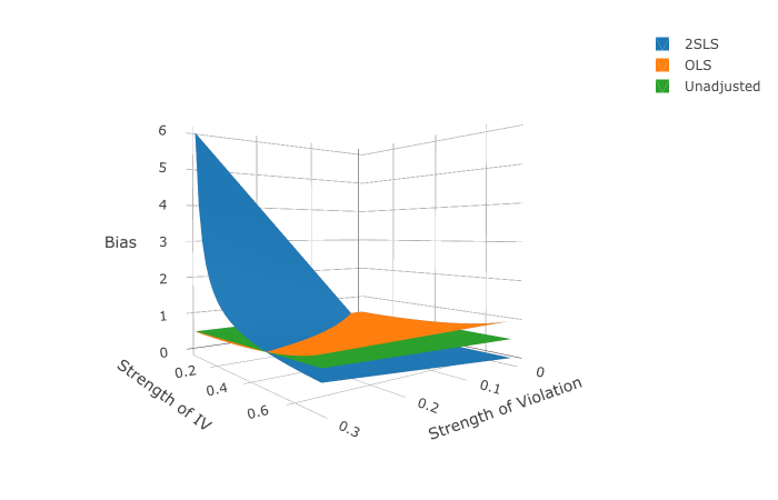
Figure 3: Analytical comparison of no adjustment, OLS adjusting for the IV, and 2SLS using the IV under varying IV strength and degree of exclusion restriction violation.

3.2 Independence Violation

Figure 4: $Z$ is Correlated with an Unobserved Confounder $U$

Figure 4 represents one violation of the independence assumption where the residual confounder $U$ is a cause of $Z$. Here, $c_{I}$ represents the degree of violation or, in this case, the effect of $U$ on $Z$. Alternative specifications create a new confounder that is only associated with $Z$ but not $X$. Nonetheless, our parameterization provides a useful case where both the independence assumption is violated and there is confounding in the relationship between $Z$ and $X$. For structural equations, we can re-use Eqs 1 and 2 as well as add an extra structural equation given by

$$Z=c_{I}U+\epsilon_{5}.$$ (10)

Proposition 3.2.

Under Eqs. (1), (2), and (10), $\hat{A}_{2}\overset{p}{\to}c_{0}+c_{1}c_{2}+c_{2}c_{3}c_{I}$, $\hat{A}_{3}\overset{p}{\to}c_{0}+\frac{c_{1}c_{2}(1-c_{I}^{2})}{1-(c_{3}+c_{1}c_{I})^{2}}$, and $\hat{A}_{4}\overset{p}{\to}c_{0}+\frac{c_{2}c_{I}}{c_{3}+c_{1}c_{I}}$.

The derivation for $A_{2}$ is a straightforward application of Wright’s path analysis so only the proofs for $A_{3}$ and $A_{4}$ are provided.[16] To better interpret these quantities, we can think about both paths on the DAG and remaining variance after orthogonalizing variables via the Frisch-Waugh-Lovell Theorem (FWL).[17] Looking at the pathways, $c_{1}c_{2}$ is the backdoor path from $X$ to $Y$ through $U$, $c_{2}c_{3}c_{I}$ is the backdoor path through $Z$, and $c_{2}c_{I}$ is the path from $Z$ to $Y$ via $U$. $c_{3}+c_{1}c_{I}$ is the unconditional correlation between $Z$ and $X$, which includes both the direct and backdoor path via $U$. $1-c_{I}^{2}$ depicts the remaining (stochastic) variation in $Z$ after orthogonalizing $U$ while $1-(c_{3}+c_{1}c_{I})^{2}$ is the remaining variance in $X$ after orthogonalizing $Z$.

Of particular interest is the trade-off between using $Z$ in 2SLS and using $Z$ in OLS. We find that adjusting for $Z$ is superior to using $Z$ for 2SLS if $\frac{c_{I}}{c_{3}+c_{1}c_{I}}>\frac{c_{1}(1-c_{I}^{2})}{1-(c_{3}+c_{1}c_{I})^{2}}$. We can begin to interpret this inequality with the reoccurring theme that if the IV is strong then attaining this inequality is more difficult: a strong IV will cause $c_{3}+c_{1}c_{I}$ to be large which inflates the inconsistency in $A_{3}$ while it decreases the consistency for $A_{4}$. The remaining variation in $Z$ not caused by $U$, or $c_{I}$, is an important quantity because as $c_{I}$ decreases, the inconsistency in $A_{3}$ will increase while the inconsistency in $A_{4}$ will decrease. In this sense, a simple sensitivity analysis procedure could be to benchmark the variation in the IV that is explained by the covariates. One could use this benchmark to conjecture how much of the variation in the IV is explained by an unobserved confounder. If this quantity is small then one could plausibly assume a fair amount of variation in $Z$ free from unobserved confounding and, thus, $c_{I}$ is small. These trade-offs can be visualized in Figure 5 where $c_{0}=0.3,c_{1}=0.7,$ and $c_{2}=0.7$.

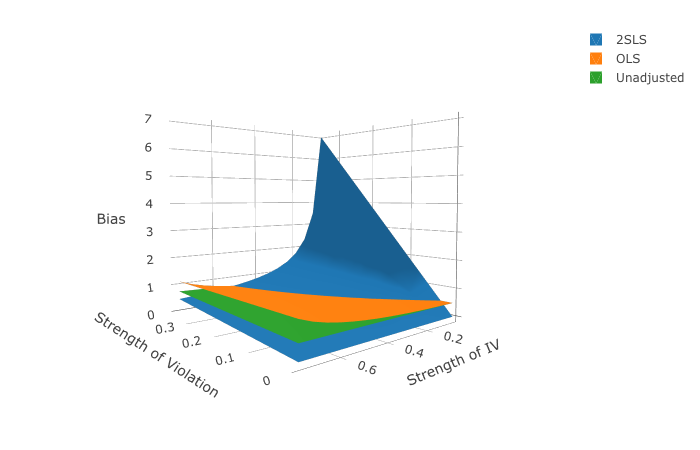
Figure 5: Analytical comparison of no adjustment, OLS adjusting for the IV, and 2SLS using the IV under varying IV strength and degree of the independence violation.

3.3 Treatment Effect Heterogeneity

We return the setting of Figure 1 where we have a perfect IV but now we omit the edge weights and introduce treatment effect heterogeneity. In this case, we do not know of any literature that gives us a salient way to to represent treatment heterogeneity using DAGs and edge weights. Therefore, the nuance is in the structural equations:

$$X=\alpha_{1}Z+\alpha_{2}U+\alpha_{3}ZU+\epsilon_{1},$$ (11)

$$Y=\beta_{1}X+\beta_{2}U+\beta_{3}XU+\epsilon_{2}.$$ (12)

The estimand of interest remains the ACE or the average of the individual treatment effects, which is denoted by $\beta_{1}$. This parameterization is consistent with a violation of Wang and Tchetgen Tchetgen (2018) assumptions 5a and 5b if $\alpha_{3}\neq 0$ and $\beta_{3}\neq 0$. The key parameter for measuring the degree of "assumption violation" is $\alpha_{3}$ because we aim to quantify how large an unobserved confounder needs to be in order to modify the effect on $Z$ in the first-stage to render $\lambda_{4}>\lambda_{3}$ and $\lambda_{4}>\lambda_{2}$, or that IVAC is inferior to CAC.

Proposition 3.3.

Under the conditions of Eqs. (11) and (12) as well as assuming $E[U^{3}]=0$, $\hat{A}_{2}\overset{p}{\to}\beta_{1}+\alpha_{2}\beta_{2}+2\alpha_{1}\alpha_{3}\beta_{3},\hat{A}_{3}\overset{p}{\to}\beta_{1}+\frac{\alpha_{2}\beta_{2}+\alpha_{1}\alpha_{3}\beta_{3}}{1-a_{1}^{2}},$ and $\hat{A}_{2}\overset{p}{\to}\beta_{1}+\frac{\alpha_{3}\beta_{3}}{\alpha_{1}}$

When comparing the relative trade-off between not adjusting for $Z$ and adjusting for $Z$, the latter is inferior if $\frac{\alpha_{2}\beta_{2}+\alpha_{1}\alpha_{3}\beta_{3}}{1-a_{1}^{2}}>\alpha_{2}\beta_{2}+2\alpha_{1}\alpha_{3}\beta_{3}$. Unlike the case of no effect modification, it is not always true that adjusting for an IV will amplify bias. Specifically, by rearranging terms we see the inequality holds if $2\alpha_{1}^{2}+\frac{\alpha_{2}\beta_{2}}{\alpha_{3}\beta_{3}}>1$. If $|\alpha_{1}|\gtrapprox 0.7$, or the IV is strongly associated with $X$, then this inequality will hold; however, this would not be the case if the IV is sufficiently weak and the multiplication of the coefficients for the interactions are larger than the multiplication of the coefficients representing the main effect.

In the more realistic case, if an analyst is aware $Z$ is an IV and assuming that the IV was sufficiently strong, the main point of concern surrounds whether the LACE estimate is more inconsistent than the ACE estimate from the unadjusted OLS. This notion is true if $\frac{\alpha_{3}\beta_{3}}{\alpha_{1}}>\alpha_{2}\beta_{2}+2\alpha_{1}\alpha_{3}\beta_{3}$ or $\frac{\alpha_{1}\alpha_{2}\beta_{2}}{\alpha_{3}\beta_{3}}+2\alpha_{1}^{2}<1$. Firstly, a strong IV, $|\alpha_{1}|\gtrapprox 0.7$, precludes this inequality from being attained. Alternatively, this inequality could fail to be attained if the ratio of main effects to interaction effects, scaled by the IV strength, is large. Setting $\alpha_{2}=0.15$, $\beta_{1}=0.1$, $\beta_{2}=0.2$, and $\beta_{3}=0.1$, we can visualize the above inequalities in Figure 6.

A final takeaway from these results is that the strength of an IV has implications on the the OLS inconsistencies even though it is independent from $U$ (e.g. via the term $2\alpha_{1}\alpha_{3}\beta_{3}$ in $A2$). Therefore, accounting for any present IVs, even if never utilized, is important for understanding the degree of inconsistency present in confounder methodology. The results of the previous three Propositions are summarized in Table 1.

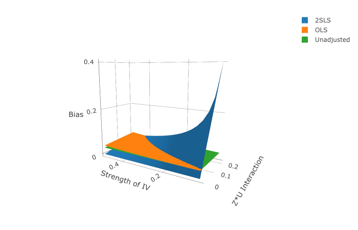
Figure 6: Analytical comparison of no adjustment, OLS adjusting for the IV, and 2SLS using the IV under varying IV strength and degree of the treatment effect heterogeneity assumption.

Table 1: Summary of Results

Scenario	$A_{2}$	$A_{3}$	$A_{4}$
No Violation
$$X=c_{1}U+c_{3}Z+\epsilon_{1}$$ $$Y=c_{0}X+c_{2}U+\epsilon_{2}$$	$c_{0}+c_{1}c_{2}$	$c_{0}+\frac{c_{1}c_{2}}{1-c_{3}^{2}}$	$c_{0}$
Exclusion Restriction Violation
$$X=c_{1}U+c_{3}Z+\epsilon_{3}$$ $$Y=c_{0}X+c_{2}U+c_{ER}Z+\epsilon_{4}.$$	$c_{0}+c_{1}c_{2}+c_{3}c_{ER}$	$c_{0}+\frac{c_{1}c_{2}}{1-c_{3}^{2}}$	$c_{0}+\frac{c_{ER}}{c_{3}}$
Independence Assumption
$$X=\alpha_{1}U+\alpha_{2}Z+\epsilon_{1}$$ $$Y=\beta X+\theta U+\epsilon_{2}$$ $$Z=c_{I}U+\epsilon_{5}.$$	$c_{0}+c_{1}c_{2}+c_{2}c_{3}c_{I}$	$c_{0}+\frac{c_{1}c_{2}(1-c_{I}^{2})}{1-(c_{3}+c_{1}c_{I})^{2}}$	$c_{0}+\frac{c_{2}c_{I}}{c_{3}+c_{1}c_{I}}$
Treatment Effect Heterogeneity
$$X=\alpha_{1}Z+\alpha_{2}U+\alpha_{3}ZU+\epsilon_{1},$$ $$Y=\beta_{1}X+\beta_{2}U+\beta_{3}XU+\epsilon_{2}.$$	$\beta_{1}+\alpha_{2}\beta_{2}+2\alpha_{1}\alpha_{3}\beta_{3}$	$\beta_{1}+\frac{\alpha_{2}\beta_{2}+\alpha_{1}\alpha_{3}\beta_{3}}{1-a_{1}^{2}}$	$\beta_{1}+\frac{\alpha_{3}\beta_{3}}{\alpha_{1}}$

3.4 Adding Additional Confounders

In the vast majority of data analyses, an analyst will have access to observed confounders that will be adjusted for to mitigate confounding both in OLS and 2SLS. Temporarily, we consider a single observed confounder, $W$, that is continuous and has mean $0$ and variance $1$. If we have multiple confounders, $\{W_{1},W_{2},...W_{J}\}$, that are in the same form as $W$, we can simply redefine $W$ as some function of the confounders, $f(W_{1},W_{2},...W_{J})$. For example, this might take a form linear combination derived from the first principal component of the $W$ matrix. Therefore, the edge weights and regression coefficients will be the joint effect of the confounders. Therefore, operationally, our updated results can accommodate multiple covariates.

Because we would like to use $W$ to benchmark relationships involving $U$, we must update the DAGs and structural equations such that $W$ has a similar form to $U$ in each assumption violation. Because of this, our previous results will change. In all cases, $W$ is orthogonal to $U$ or, in other words, $U$ represents confounding in ACE unrelated to $U$. With the exception of $A_{1}$, the quantities of interest are updated to

$$A_{2} =\frac{\partial}{\partial x}E[Y|x,w]$$ (13)

$$A_{3} =\frac{\partial}{\partial x}E[Y|x,z,w]$$ (14)

$$A_{4} =\frac{Cov(Y,Z|W)}{Cov(X,Z|W)}=\frac{\frac{\partial}{\partial z}E[Y|z,w]}{\frac{\partial}{\partial z}E[X|z,w]}.$$ (15)

3.4.1 Exclusion Restriction

Figure 7 serves as an example of a covariate that has no direct impact on $Z$ or $U$. Nevertheless, if we were to condition upon $X$ and nothing else, $U$ would no longer be independent of $W$ or $Z$ due to the collider effect. A collider effect induces an association between two variables that point to (i.e. cause) a single variable that has been conditioned.[15] However, conditioning upon $W$ breaks this association.

Figure 7: A DAG with observed confounder and violation of exclusion restriction ($W$).

The updated structural equations are

$$X=c_{1}U+c_{3}Z+c_{5}W+\epsilon_{3}$$ (16)

$$Y=c_{0}X+c_{2}U+c_{ER}Z+c_{6}W+\epsilon_{4}.$$ (17)

Proposition 3.4.

Under Eqs. (16) and (17)$,\hat{A}_{2}\overset{p}{\to}c_{0}+\frac{c_{1}c_{2}+c_{3}c_{ER}}{1-c_{5}^{2}}$ and $\hat{A}_{3}\overset{p}{\to}c_{0}+\frac{c_{1}c_{2}}{1-c_{3}^{2}-c_{5}^{2}}$

The proof is very similar to that of Proposition 3.1 so it is omitted. As expected, adjusting for $W$ leads to decreased variance in $X$, which leads to a higher proportional contribution of $U$, at the benefit of eliminating the backdoor path via $c_{5}c_{6}$. For 2SLS, the results for $A_{4}$ are not affected because the assumption violations vis-a-vis using $Z$ as an IV are not influenced by $W$. Nevertheless, in practical settings, adjusting for $W$ will usually increase precision of $\hat{A}_{4}$.

3.4.2 Independence

Figure 8: $W$ mimics $U$ in the DAG.

Besides introducing $W$ as a confounder in the $X-Y$ relationship, Figure 8 extends $W$ to be a confounder in the $Z-Y$ and $Z-X$ relationships. Therefore, the validity of $Z$ as an IV is contingent on conditioning upon both $W$ and $Z$. Thus, the structural equations are updated to

$$Z=c_{I}U+c_{7}W+\epsilon_{5}$$ (18)

$$X=c_{1}U+c_{3}Z+c_{5}W+\epsilon_{1},$$ (19)

$$Y=c_{0}X+c_{2}U+c_{6}W+\epsilon_{2}.$$ (20)

The results for all quantities, $A_{2}$, $A_{3}$, and $A_{4}$, can now be updated per the following proposition:

Proposition 3.5.

Under Eqs. (19), (20), and (18):

$$\hat{A}_{2}\overset{p}{\to}c_{0}+\frac{c_{1}c_{2}+c_{2}c_{3}c_{I}}{1-(c_{5}+c_{3}c_{7})^{2}},$$ (21)

$$\hat{A}_{3}\overset{p}{\to}c_{0}+\frac{\frac{c_{1}c_{2}(1-c_{7}^{2}-c_{I}^{2})}{1-c_{7}^{2}}}{1-(c_{5}+c_{3}c_{7})^{2}-(1-c_{7}^{2})(c_{3}+\frac{c_{1}c_{I}}{1-c_{7}^{2}})^{2}},$$ (22)

$$\hat{A}_{4}\overset{p}{\to}c_{0}+\frac{c_{2}c_{I}}{(1-c_{7}^{2})(c_{3}+\frac{c_{1}c_{I}}{(1-c_{7}^{2})})}.$$ (23)

These results bear some resemblance to Proposition 3.2 when we did not have $W$ present. For $A_{2}$, in the numerator, because $W$ does not mitigate the influence of $U$ in the DAG, we still have two backdoor paths from $X$ to $Y$ that go through $U$. Meanwhile, in the denominator the variance of $X$ is reduced via controlling for $W$, which has a direct path to $X$ as well as an indirect path via $Z$.

For $A_{3}$, the quantity is similar conceptually to our findings in Proposition 3.2 except that we must additionally account for controlling for $W$. In the numerator, $c_{1}c_{2}(1-c_{7}^{2}-c_{I}^{2})$ represents the magnitude of unobserved confounding reduced (i.e. multiplied) by the exogenous variance of $Z$ due to there no longer being a backdoor path to $Y$ via $Z$. We must account for the cost of adjusting $W$ therefore this quantity is amplified (i.e. divided) by $1-c_{7}^{2}$, the variance in $Z$ free of $W$. In the denominator, we have the remaining variance of $X$ after adjusting for $W$ and $Z$. The first subtracting term represents the unconditional $R^{2}$ between $X$ and $Z$ while the second takes the variation of $Z$ free of $W$ and multiplies it by the partial $R^{2}$ between $Z$ and $X$, adjusting for $W$. Because we haven’t adjusted for $U$, the backdoor path via $U$ remains and, furthermore, because $W$ does not mitigate this, $W$ essentially acts like a bias amplifier for $c_{1}c_{I}$. Lastly, $A_{4}$ represents the association between $Z$ and $X$ via $U$ as well as the variation exogenous from $W$ directly from $Z$.

3.4.3 Treatment Effect Heterogeneity

Because we require our observed confounder to be of the same form of $U$ for benchmarking purposes, we will set $W$ as both an effect modifier of the treatment on the outcome and of the instrument on the treatment assignment with the following structural equations:

$$X=\alpha_{1}Z+\alpha_{2}U+\alpha_{3}ZU+\alpha_{4}W+\alpha_{5}ZW+\epsilon_{1},$$ (24)

$$Y=\beta_{1}X+\beta_{2}U+\beta_{3}XU+\beta_{4}W+\beta_{5}XW+\epsilon_{2}.$$ (25)

The presence of $XW$, which is observed but still endogenous, means that in OLS, we must adjust for it and in 2SLS, must provide an an additional IV. In particular, we will choose $ZW$. Therefore we modify the quantities of interest to

$$A_{2} =\frac{\partial}{\partial x}E[Y|x,w,xw]$$ (26)

$$A_{3} =\frac{\partial}{\partial x}E[Y|x,z,w,xw]$$ (27)

$$A_{4} =\frac{\partial}{\partial\hat{x}}E[Y|\hat{x},\widehat{xw},w]$$ (28)

where $\hat{x}$ and $\widehat{xw}$ represent the fitted values from using $Z$, $ZW$, and $W$ as regressors for $X$ and $XW$, respectively. Note that now the main effect is obtained after orthogonalizing $XW$ and $W$, or $\widehat{XW}$ and $W$ in 2SLS, which we can find via FWL by treating $XW$ as any other covariate. Therefore, the corresponding interpretation of the main effect is when $W=0$, or we are at the average value of the covariate due to centering the variable.

Proposition 3.6.

Under Eqs. (24) and (25) as well as $E[U^{3}]=0$, $E[W^{3}]=0$, $E[W^{4}]=3$, and $E[U^{4}]=3$ we have $\hat{A}_{2}\overset{p}{\to}\beta_{1}+\frac{\alpha_{2}\beta_{2}+2\alpha_{1}\alpha_{3}\beta_{3}}{1-\alpha_{4}^{2}-\frac{4\alpha_{1}^{2}\alpha_{5}^{2}}{1+\alpha_{4}^{2}+2\alpha_{5}^{2}}}$ and $\hat{A}_{4}\overset{p}{\to}\beta_{1}+\frac{\alpha_{1}\alpha_{3}\beta_{3}-\frac{2\alpha_{1}\alpha_{3}\alpha_{5}^{2}\beta_{3}}{\alpha_{1}^{2}+\alpha_{5}^{2}}}{\alpha_{1}^{2}+\alpha_{5}^{2}-\frac{4\alpha_{1}^{2}\alpha_{5}^{2}}{(\alpha_{1}^{2}+\alpha_{5}^{2}})}$.

The interpretation of $A_{2}$ is consistent with Proposition 3.3 with the denominator reflecting the fact that we are adjusting for $W$ and $XW$, which reduces the remaining variance of $X$. For $A_{4}$, because we are no longer computing the ratio of coefficients the interpretation is not directly comparable to Proposition 3.3. Nevertheless, we can see the influence of the $Z-U$ interaction on the inconsistency and observe that because $\hat{XU}$ is correlated with $\widehat{XW}$, adjusting for $\widehat{XW}$ will reduce the influence of $\widehat{XU}$, hence the subtraction terms.

One may notice that we have omitted the derivation for the result of $A_{3}$ and this is because we only wish to compare $A_{2}$ and $A_{4}$. From our discussion of Proposition 3.3, assuming $sign(\alpha_{2}\beta_{2})=sign(\alpha_{3}\beta_{3})$ for sake of simplicity, bias amplification will hold in the effect modification case if $2\alpha_{1}^{2}+\frac{\alpha_{2}\beta_{2}}{\alpha_{3}\beta_{3}}>1$. When we have a strong IV, or $|\alpha_{1}|\gtrapprox 0.7$, then this inequality holds. If we instead lower the strength of the IV to where we must consider $\frac{\alpha_{2}\beta_{2}}{\alpha_{3}\beta_{3}}>1-2\alpha_{1}^{2}$, we would require the multiplication interaction effects to be at least as large as the main effects with this requirement increasing as the IV strength increases. We argue that in this circumstance one should avoid using $Z$ altogether because concern over this ratio would imply that the IV is weak and the LACE is likely to be far from the ACE due to large heterogeneity. Thus, a comparison between OLS and 2SLS is not warranted. As we will describe later on, one may "benchmark" this ratio using the observed confounders and instrument as an initial check if an IV is appropriate in their circumstance for targeting the ACE.

4 Sensitivity Analysis

In this section, we use the closed form derivations of the previous section to develop a set of sensitivity analysis procedures that provide analysts with information surrounding whether OLS or 2SLS may be more appropriate given the observed data and hypothesized assumption violations. We focus on comparing $A_{3}$ and $A_{4}$, or using $Z$ as a confounder versus as an IV, by graphically presenting the relative inconsistency $\frac{\lambda_{4}}{\lambda_{3}}$ as measured by the degree of IV assumption violations and unobserved confounding.

The graphical depiction of the relative inconsistencies is largely motivated by Cincelli and Hazlett (2020) [18] and Cincelli and Hazlett (2022)[10] where they use a set of partial $R^{2}$’s to characterize how large the assumption violations in confounder and 2SLS analyses must be to render statistically significant results null. Instead of focusing on hypothesis testing, however, we examine how large unobserved confounding and the IV assumption violations could be in order for $\frac{\lambda_{4}}{\lambda_{3}}>1$ or $\frac{\lambda_{4}}{\lambda_{3}}<1$. Following this, like Cincelli and Hazlett, we use benchmarking to estimate the unobserved sensitivity quantities across a variety of scenarios.

To briefly summarize the benchmarking procedure, suppose we have the quantity $R^{2}_{Y\sim U|X,W}$, or the additional gain in $R^{2}$ by adding $U$ to the regression of $Y$ on treatment $X$ and observed covariate $W$. We must assume that for the individual confounders that make up the composite confounder $W$, the magnitude of the $W_{j}-X$ relationship and $W_{j}-Y$ relationship for $j\in\{1,2,...J\}$ are similar to the magnitude of the $U-X$ and $U-Y$ relationship, respectively. As a result, we can therefore benchmark $R^{2}_{Y\sim U|X,W}$ as conservatively as possible with a quantity such as $\max_{j}R^{2}_{Y\sim W_{j}|X,\mathcal{W}_{-j}}$ where $W_{-j}$ represents all other observed confounders besides $W_{j}$. In the remainder of this section, we will focus on the sensitivity analysis procedure in the scenario of the exclusion restriction. Then, using the same principles, present the results for the independence and heterogeneity assumption violations more succinctly.

4.1 Exclusion Restriction Violation

Proposition 4.1.

$\lambda_{4}=\frac{|c_{4}|}{|c_{3}|}=\frac{c_{1}c_{2}}{1-c_{3}^{2}-c_{5}^{2}}=\lambda_{3}$ can be re-written as $\frac{\sqrt{R^{2}_{Y\sim Z|X,U,W}}\sqrt{1-R^{2}_{Y\sim U|X,W}}(1-R^{2}_{X\sim W+Z})}{\sqrt{1-R^{2}_{Y\sim Z|X,W}}\sqrt{R^{2}_{X\sim Z}}sd(Z^{\perp X,W})}>\frac{\sqrt{R^{2}_{X\sim U}R^{2}_{Y\sim U|X,W,Z}}}{\sqrt{1-R^{2}_{U\sim X|W,Z}}}$ where $sd(Z^{\perp X,W})$ is the standard deviation resulting from the residuals of regressing $Z$ on $X$ and $W$.

In order to simplify the description of the above quantity, we will decompose the terms in the above inequality into three factors: symbolically, we let

$$\phi =\frac{1-R^{2}_{X\sim W+Z}}{\sqrt{1-R^{2}_{Y\sim Z|X,W}}\sqrt{R^{2}_{X\sim Z}}sd(Z^{\perp X,W})}$$ (29)

$$\gamma =\frac{\sqrt{R^{2}_{X\sim U}}\sqrt{R^{2}_{Y\sim U|X,W,Z}}}{\sqrt{1-R^{2}_{U\sim X|W,Z}}\sqrt{1-R^{2}_{Y\sim U|X,W}}}$$ (30)

$$\theta =\sqrt{R^{2}_{Y\sim Z|X,W,U}}.$$ (31)

Here, $\phi$ represents all observed quantities that can be directly estimated, $\gamma$ is a function that is monotonically increasing as the unobserved confounding increases, and $\theta$ is the degree of the exclusion restriction violation. We will need to benchmark $\gamma$ and $\theta$, which we will refer to as $\gamma^{B}$ and $\theta^{B}$. These observed benchmarks are detailed in Table 2.

Table 2: Benchmarking for $\gamma$ and $\theta$ Quantities for Exclusion Restriction

Quantity	Benchmark
$R^{2}_{Y\sim Z|X,W,U}$	$R^{2}_{Y\sim Z|X,W}$
$R^{2}_{X\sim U}$	$\max_{j}R^{2}_{X\sim W_{j}}$
$R^{2}_{Y\sim U|X,W,Z}$	$\max_{j}R^{2}_{Y\sim W_{j}|X,\mathcal{W}_{-j},Z}$
$R^{2}_{U\sim X|W,Z}$	$\max_{j}R^{2}_{W_{j}\sim X|\mathcal{W}_{-j},Z}$
$R^{2}_{Y\sim U|X,W}$	$\max_{j}R^{2}_{Y\sim W_{j}|X,\mathcal{W}_{-j}}$

We begin our sensitivity analysis procedure with ambivalence between OLS and 2SLS, or that $\frac{\lambda_{4}}{\lambda_{3}}=1\implies\frac{\theta\phi}{\gamma}=1$. Then, given $\hat{\phi}$ and $\theta^{B}$, we can solve for how large $\gamma$, or the degree of unobserved confounding, must be in order for the equality to be maintained. We call this $\gamma^{I}$ where "I" indicates the $\gamma$ "implied" by assuming ambivalence. $\gamma^{I}$ serves as an anchor point for the next step when we compute $\gamma^{B}$.

Now using the data, we will find $\gamma^{B}$ through benchmarking and combine this with $\phi$ and $\theta_{B}$ to form $\frac{\theta^{B}\phi}{\gamma^{B}}$. We will refer to this fraction as the "inconsistency ratio," or "IR", which may be used to judge the use of 2SLS or OLS. For example, a ratio of $<1$ implies that $\lambda_{3}>\lambda_{4}$ and suggests that we should use 2SLS as opposed to OLS. Of course, the degree of unobserved confounding could be different than the observed benchmark. To mitigate this, we may additionally add a multiplier, $M*\gamma^{B}$, if we believe the observed confounders underestimate ($M<1$) or overestimate ($M>1$) the degree of unobserved confounding. For example, if $M=0.5$, we are assuming that the unobserved confounding is half as much as the benchmarked confounding. Lastly, we compute $\theta^{I}$ or the degree of the exclusion restriction violation to satisfy $\frac{\theta^{I}\phi^{B}}{\gamma^{B}}=1$, or returning to ambivalence.

The above quantities culminate in the graphical visualization in Figure 9. This Figure was produced under a simulation where $\frac{\lambda_{4}}{\lambda_{3}}<1$, implying that 2SLS is a better choice than OLS in reducing inconsistency for the ACE. The x-axis shows the IR, while the y-axis tells us the degree of unobserved confounding as captured by $\gamma$. Focusing on the y-axis, the position of the black dotted line, our anchor point, gives us the plausibility of $\gamma^{I}$ by comparing to $0.5\times\gamma_{B}$ (red), $\gamma_{B}$ (purple), and $1.5\times\gamma_{B}$ (blue). We can see that the degree of unobserved confounding required for ambivalence is roughly 60% of the benchmarked confounding. We obtain 60% by comparing the y-intercept of the purple line ($\approx$ 0.25) with the y-intercept of the dotted black line ($\approx$ 0.15). Looking at the x-axis, this works in favor of 2SLS as the corresponding inconsistency calculated by $\frac{\theta^{B}\phi^{B}}{\gamma^{B}}<1$ unless the true degree of unobserved confounding is less than that of the benchmarked $\gamma$.

Lastly, we will address the legend labels for which we have one for each line. "Benchmarked ER Violation" is the benchmarked exclusion restriction violation as quantified by $R^{2}_{Y\sim Z|X,W,U}$ while "ER Violation Required" tells us the value of $R^{2}_{Y\sim Z|X,W,U}$ required to return to ambivalence at the given multiplier. The comparison of the required numbers and the benchmarked violation gives analysts information to judge the plausibility of ambivalence. For example, on Figure 9, the degree violation required to return to ambivalence given $M=1$ (0.061) is roughly 2.3 times the observed benchmark of 0.026.

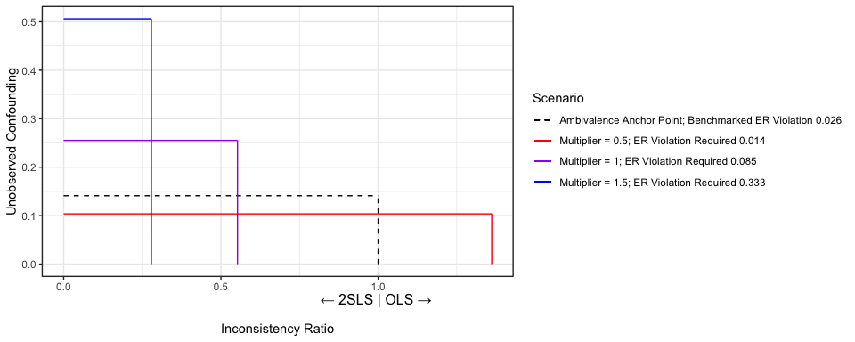
Figure 9: A case where the inconsistency of OLS is more than that of 2SLS under an exclusion restriction violation

4.2 Independence Violation

Proposition 4.2.

$\lambda_{4}=\Big{|}\frac{c_{2}c_{I}}{c_{3}(1-c_{7}^{2})+c_{1}c_{I}}\Big{|}=\Big{|}\frac{\frac{c_{1}c_{2}(1-c_{7}^{2}-c_{I}^{2})}{1-c_{7}^{2}}}{1-(c_{5}+c_{3}c_{7})^{2}-(1-c_{7}^{2})(c_{3}+\frac{c_{1}c_{I}}{1-c_{7}^{2}})^{2}}\Big{|}=\lambda_{3}$ can be re-written as $\frac{\sqrt{R^{2}_{Z\sim U}}}{\sqrt{1-R^{2}_{Z\sim U|W}}}=\sqrt{R^{2}_{X\sim U|Z,W}}\Bigg{[}\frac{\sqrt{R^{2}_{X\sim Z|W}}sd(X^{\perp Z,W})sd(X^{\perp W})sd(Z^{\perp W})}{1-R^{2}_{X\sim W}-(1-R^{2}_{Z\sim W})R^{2}_{X\sim Z|W}}\Bigg{]}$

Once again, we partition the quantities in Proposition as follows:

$$\phi =\frac{\sqrt{R^{2}_{X\sim Z|W}}sd(X^{\perp Z,W})sd(X^{\perp W})sd(Z^{\perp W})}{1-R^{2}_{X\sim W}-(1-R^{2}_{Z\sim W})R^{2}_{X\sim Z|W}}$$ (32)

$$\gamma =\sqrt{R^{2}_{X\sim U|Z,W}}$$ (33)

$$\theta =\frac{\sqrt{R^{2}_{Z\sim U}}}{\sqrt{1-R^{2}_{Z\sim U|W}}}$$ (34)

$$R^{2}_{Z\sim U} =\frac{\phi^{2}\gamma^{2}(1-R^{2}_{Z\sim W})^{2}}{1+\phi^{2}\gamma^{2}}$$ (35)

The IR in this case will be $\frac{\phi\gamma}{\theta}$ with $\theta$ being a monotonic function with the degree of the independence violation increasing. Though we may solve for $R^{2}_{Z\sim U}$, as in line 35, we leave $\theta$ in its current form to maintain the clean interpretation $\gamma$. Then, given a value for $\gamma$, $\phi$, and the observed $R^{2}_{Z\sim W}$, we calculate the value of $R^{2}_{Z\sim U}$ in the legend entry for the corresponding line in the sensitivity plot. An example of the sensitivity plot for the independence violation is presented in Figure 10. The construction and interpretation of this figure is the same as in the exclusion restriction violation except for the fact that we now measure how large does an independence violation need to be to return to ambivalence. This is denoted by "U-Z B" and "U-Z Req." as in the $R^{2}$ magnitude of the edge from $U$ to $Z$ as in the DAG in Figure 8. In this case, we simulated the data such that $\lambda_{4}=\lambda_{3}$ so the purple line (multiplier of 1) and the required violation is close to the black anchor line and the observed benchmark. The corresponding benchmarks are detailed in Table 3.

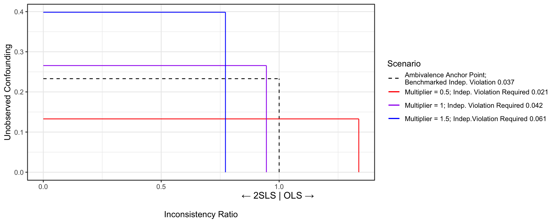
Figure 10: A case where the inconsistency of OLS is roughly equal to that of 2SLS under an independence violation

Table 3: Benchmarking for $\gamma$ and $\theta$ Quantities for Independence Violation

Quantity	Benchmark
$R^{2}_{X\sim U|Z,W}$	$\max_{j}R^{2}_{X\sim W_{j}|\mathcal{W}_{-j},Z}$
$R^{2}_{Z\sim U}$	$\max_{j}R^{2}_{Z\sim W_{j}}$
$R^{2}_{Z\sim W}$	$\max_{j}R^{2}_{Z\sim W_{j}|\mathcal{W}_{-j}}$

4.3 Treatment Effect Heterogeneity

Proposition 4.3.

$\lambda_{2}=\beta_{1}+\frac{\alpha_{2}\beta_{2}+2\alpha_{1}\alpha_{3}\beta_{3}}{1-\alpha_{4}^{2}-\frac{4\alpha_{1}^{2}\alpha_{5}^{2}}{1+\alpha_{4}^{2}+2\alpha_{5}^{2}}}$ and $\lambda_{4}=\frac{\alpha_{1}\alpha_{3}\beta_{3}-\frac{2\alpha_{1}\alpha_{3}\alpha_{5}^{2}\beta_{3}}{\alpha_{1}^{2}+\alpha_{5}^{2}}}{\alpha_{1}^{2}+\alpha_{5}^{2}-\frac{4\alpha_{1}^{2}\alpha_{5}^{2}}{(\alpha_{1}^{2}+\alpha_{5}^{2}})}$ can be rewritten as

$$\Bigg{|}\frac{1/2-\frac{R^{2}_{X\sim ZW}}{Var(\hat{XW})}}{R^{2}_{X\sim W}+R^{2}_{X\sim ZW}-R^{2}_{XW\sim X}}\Bigg{|}Var(X^{\perp W,XW})$$ (36)

$$=\Bigg{|}\frac{\sqrt{R^{2}_{X\sim U}}\sqrt{R^{2}_{Y\sim U|X,W,XU,XW}}}{2\sqrt{R^{2}_{X\sim Z}}\sqrt{R^{2}_{X\sim ZU}}\sqrt{R^{2}_{Y\sim XU|X,W,U,XW}}}$$ (37)

$$\frac{\sqrt{1-R^{2}_{Y\sim XU|X,W,XW}}\sqrt{1-R^{2}_{XU\sim U|W,XW}}\sqrt{1-R^{2}_{XW\sim XU}}}{\sqrt{1-R^{2}_{Y\sim XU|X,W,XW}}\sqrt{1-R^{2}_{U\sim X}}}sign(\beta_{2}\alpha_{2})+sign(\alpha_{1}\alpha_{3}\beta_{3})\Bigg{|}$$ (38)

Note that because we are using $A_{2}$ to measure the CAC, $\lambda_{2}$ represents the inconsistency. Our partitioned quantities are as follows

$$\phi_{1} =\Bigg{|}\frac{1/2-\frac{R^{2}_{X\sim ZW}}{Var(\hat{XW})}}{R^{2}_{X\sim W}+R^{2}_{X\sim ZW}-R^{2}_{XW\sim X}}\Bigg{|}Var(X^{\perp W,XW})$$ (39)

$$\phi_{2} =2\sqrt{R^{2}_{X\sim Z}}$$ (40)

$$\gamma_{1} =\frac{\sqrt{R^{2}_{X\sim U}}\sqrt{R^{2}_{Y\sim U|X,W,XU,XW}}}{\sqrt{1-R^{2}_{Y\sim U|X,W,XW}}\sqrt{1-R^{2}_{X\sim U}}}$$ (41)

$$\gamma_{2} =\frac{\sqrt{1-R^{2}_{Y\sim XU|X,W,XW}}\sqrt{1-R^{2}_{XU\sim U|W,XW}}\sqrt{1-R^{2}_{XW\sim XU}}}{\sqrt{R^{2}_{Y\sim XU|X,W,U,XW}}}$$ (42)

$$\theta =\sqrt{R^{2}_{X\sim ZU}}.$$ (43)

We divide $\phi$ into $\phi_{1}$ and $\phi_{2}$ because the sign of $sign(\phi_{2})$ may change with what the analyst will impute for $sign(\alpha_{2}\beta_{2})$ and $sign(\alpha_{1}\alpha_{3}\beta_{3})$. We initially will discuss the case where $sign(\alpha_{2}\beta_{2})=sign(\alpha_{1}\alpha_{3}\beta_{3})$ and then further expand upon the more complicated cases. $\gamma$ is essentially divided into two parts: quantities related to the main effect of unobserved confounding ($\gamma_{1}$) and quantities related to treatment effect heterogeneity ($\gamma_{2}$). To maintain a consistent interpretation of weighing potential unobserved confounding in OLS to assumption violations in 2SLS across our suite of sensitivity analysis tools, we will only put multipliers on the main effects of $U$ or $\gamma_{1}$. Therefore, holding treatment effect heterogeneity constant, $\gamma=\gamma_{1}\gamma_{2}$ is a monotonically increasing function of the strength of unobserved confounding. Lastly, $\theta$ quantifies the degree of violation of the IV assumption of treatment effect heterogeneity by measuring the $R^{2}$ of the interaction between the unobserved confounder in the first stage.

Under our sign assumptions, the IR is defined as $\frac{(\phi_{1}-1)\phi_{2}\theta}{M\gamma_{1}\gamma_{2}}$ where $M$ is the multiplier on benchmarked residual confounding. Figure 11 shows an example plot where $\lambda_{4}>\lambda_{2}$. In other words, this depicts the case where the interaction in the first stage between the instrument and unobserved effect modifier is large enough such that the inconsistency of LACE for the ACE is larger than OLS under unobserved confounding. As such, the required magnitude of this interaction is less than that of the benchmark. We define the benchmarking quantities in Table 4.

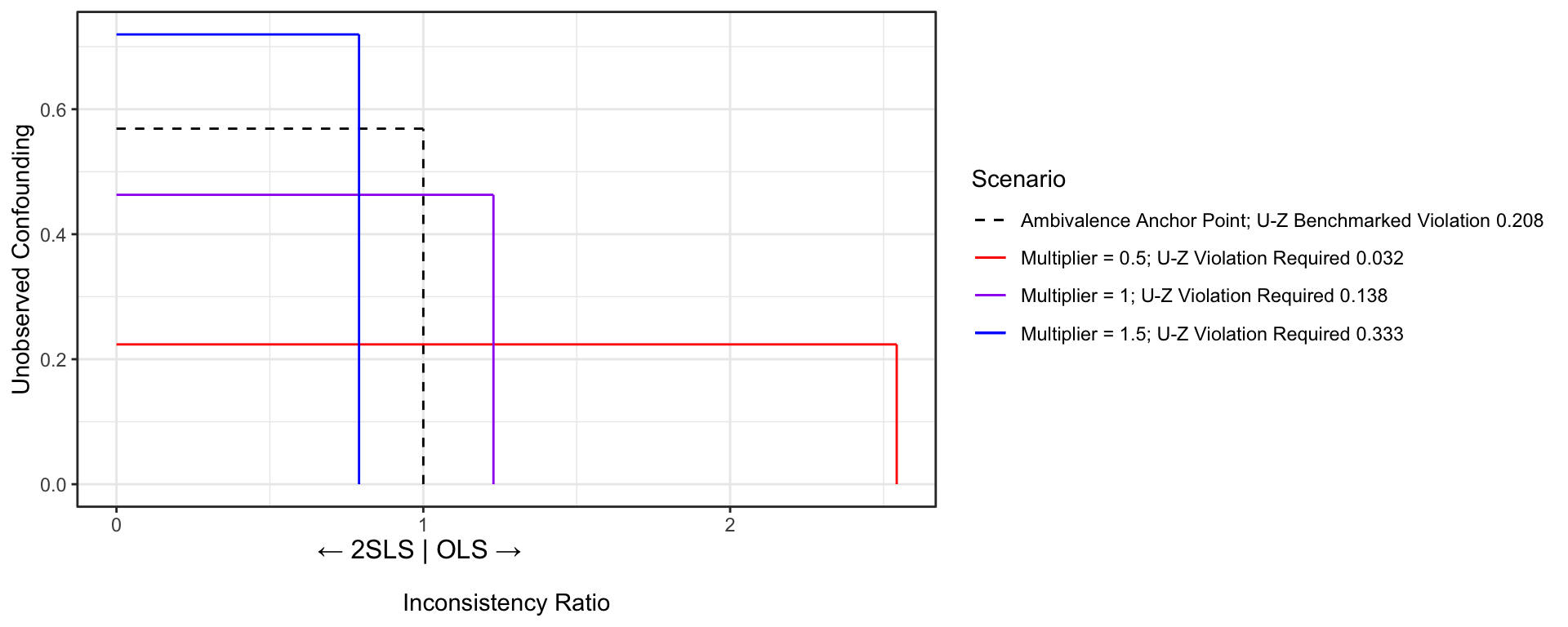
Figure 11: A case where the inconsistency of OLS is less than that of 2SLS under a treatment effect heterogeneity violation

Table 4: Benchmarking for $\gamma$ and $\theta$ Quantities for Treatment Effect Heterogeneity

Quantity	Benchmark
$R^{2}_{X\sim U}$	$\max_{j}R^{2}_{X\sim W_{j}}$
$R^{2}_{Y\sim U|X,W,XU,XW}$	$\max_{j}R^{2}_{Y\sim W_{j}|X,\mathcal{W}_{-j},XW}$
$R^{2}_{Y\sim U|X,W,XW}$	$\max_{j}R^{2}_{Y\sim W_{j}|X,\mathcal{W}_{-j},XW}$
$R^{2}_{Y\sim XU|U,X,W,XW}$	$\max_{j}R^{2}_{Y\sim XW_{j}|X,W,X\mathcal{W}_{-j}}$
$R^{2}_{Y\sim XU|X,W,XW}$	$\max_{j}R^{2}_{Y\sim XW_{j}|X,W,X\mathcal{W}_{-j}}$
$R^{2}_{XU\sim U|W,XW}$	$\max_{j}R^{2}_{XW_{j}\sim W_{j}|\mathcal{W}_{-j},X\mathcal{W}_{-j}}$
$R^{2}_{XW\sim XU}$	$\max_{i\neq j}R^{2}_{XW_{i}\sim XW_{j}}$
$R^{2}_{X\sim ZU}$	$\max_{j}R^{2}_{X\sim ZW_{j}}$

Now, we will address the case where it may not necessarily be true that $sign(\alpha_{2}\beta_{2})=sign(\alpha_{1}\alpha_{3}\beta_{3})$. Although we know $sign(\alpha_{1})$, we do not know the signs of the remaining coefficients, which are associated with $U$. Though there may be many combinations of what the signs of the individual coefficients may be, there are only three possible IRs

$$IR=\begin{cases*}\frac{(\phi_{1}-1)\phi_{2}\theta}{M\gamma_{1}\gamma_{2}}&if $sign(\alpha_{2}\beta_{2})=sign(\alpha_{1}\alpha_{3}\beta_{3})$,\\ \frac{(\phi_{1}+1)\phi_{2}\theta}{M\gamma_{1}\gamma_{2}}&if $sign(\alpha_{2}\beta_{2})\neq sign(\alpha_{1}\alpha_{3}\beta_{3})$ and $\frac{|\alpha_{2}\beta_{2}|}{|\alpha_{3}\beta_{3}|}>|2\alpha_{1}|$,\\ -\frac{(\phi_{1}-1)\phi_{2}\theta}{M\gamma_{1}\gamma_{2}}&if $sign(\alpha_{2}\beta_{2})\neq sign(\alpha_{1}\alpha_{3}\beta_{3})$ and $\frac{|\alpha_{2}\beta_{2}|}{|\alpha_{3}\beta_{3}|}\leq|2\alpha_{1}|$.\end{cases*}$$

Practically, there are only two IRs for us to consider because the first and third cases are opposite signs and we are concerned with the magnitude of the IR rather than the sign. Whether the condition of $\frac{|\alpha_{2}\beta_{2}|}{|\alpha_{3}\beta_{3}|}>|2\alpha_{1}|$ is met can be investigated through benchmarking. As an example of this condition, suppose $\alpha=0.5$ – a fairly strong instrument in this context – then we require the treatment effect heterogeneity, $\alpha_{3}\beta_{3}$, to be no stronger than the effect of $U$ on $X$ when $Z=0$ ($\alpha_{2}$) as well as $U$ on $Y$ when $X=0$ ($\beta_{2}$). Note that because $X$ and $Z$ are centered, $\alpha_{2}$ and $\beta_{3}$ are at the average value of these variables. We suggest that two graphs are computed for both cases and, following this, if the conclusions agree, then no further action should be taken. If they disagree, then one may benchmark the condition to give a sense of which condition is more likely or, alternatively, average the ICs assuming equal probability of each case.

5 Simulation

In this section, we present results verifying the closed form derivations for all three assumption violation scenarios with and without covariates. Additionally, we further present the use of our sensitivity analysis procedure. All variables were generated via the structural equations provided in the earlier sections with the error terms following a normal distribution with mean zero. When the variables were independent from all other variables in the system, such as $U$, they were standard normal. When the variable was determined by other variables in the system, such as $X$, it was still normal but with the variance of the error term being equal to one minus the variance of the other variables in the structural equation. This is so that the total variance of terms like $Var(X)$ will still equal one (see the "Notes about Simulations" section in the appendix). For example, in Eq 1, $\sigma_{\epsilon_{1}}=1-c_{1}^{2}-c_{3}^{2}$ and, thus, $\epsilon_{1}\sim N(0,1-c_{1}^{2}-c_{3}^{2})$.

To obtain the simulated numbers for OLS, we use the built-in lm from R function while for 2SLS, we use the ivreg function from the ivreg R package. In the exclusion restriction and independence setting, we present the Monte Carlo averages over 500 simulations of 500 observations generated. For treatment effect heterogeneity because the empirical results take more samples to converge, we used 500 simulations of 3000 observations. Note that for all simulations, for demonstration purposes, we set the IV to be sufficiently strong such that the estimates would converge on the population value within a reasonable sample size. Nevertheless, our results otherwise hold for weak IVs if the number of observations in each simulation increased significantly.

To demonstrate the sensitivity analysis plots, we used one generation from the relevant set of structural equations with a sample size of 500 for the exclusion restriction and independence violations while we have a sample size of 1000 for the heterogeneity violation. To simulate a set of covariates that we may use to benchmark the unobserved quantities, we generated three independent covariates ($W_{1},W_{2},W_{3}$) from a standard normal distribution and constructed $W$ via the first principal component.

5.1 Exclusion Restriction

For the case with no covariates, we set the following structural parameters $c_{0}=0.3$, $c_{1}=0.5$, $c_{2}=0.5$, $c_{3}=0.5$, and $c_{ER}=0.25$. For the case with covariates, we have $c_{0}=0.25$, $c_{1}=0.4$, $c_{2}=0.4$, $c_{3}=0.7$, $c_{ER}=0.25$, $c_{5}=0.4$, and $c_{6}=0.4$. The results are presented in Table 5.

Table 5: Theoretical and Simulated Results for the Exclusion Restriction Violation

		Method
		OLS without Z	OLS with Z	2SLS with Z
Without covariates	Closed Form Result	0.375	0.333	0.5
	Simulated Result	0.374	0.334	0.496
With covariates	Closed Form Result	0.399	0.457	0.357
	Simulated Result	0.398	0.459	0.354

Using the values $c_{1}=c_{2}=c_{5}=c_{6}=0.4$ and $c_{3}=0.3$, an IV of relative moderate strength, we present how the sensitivity plots change in response to an increasing exclusion violation in Figure 12. We see that since the IV is not very strong, it will take only a small degree of the exclusion restriction violation to reach ambivalence and suggest that OLS is more appropriate. Note that for cases that there is no violation, benchmarking will pick up a small signal so the IC will not be 0 though small.

Figure 12: Increasing Exclusion Restriction Violation Sensitivity Analysis Results with Benchmarking

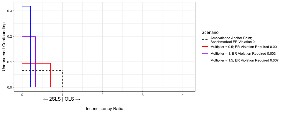
(a) $c_{ER}=0$ (no violation); True IR = 0

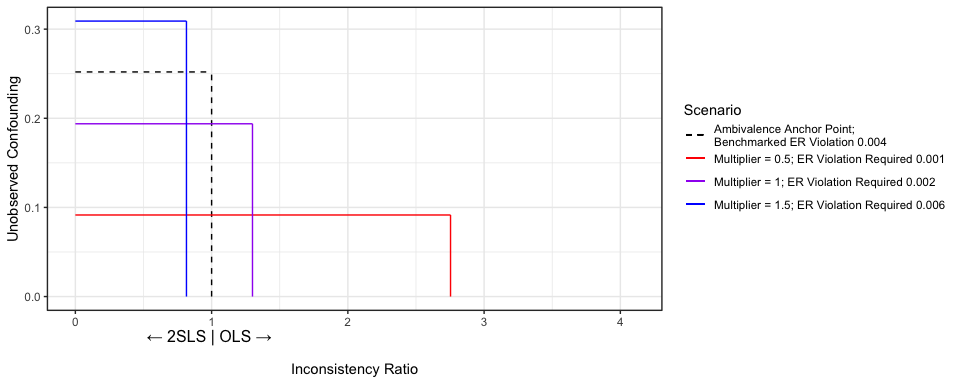
(b) $c_{ER}=0.07$; True IR = 1.09

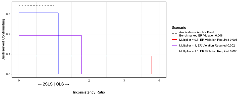
(c) $c_{ER}=0.09$; True IR = 1.4

5.2 Independence

For the case with no covariates, we set the following structural parameters $c_{0}=0.3$, $c_{1}=0.5$, $c_{2}=0.5$, $c_{3}=0.5$, $c_{ER}=0.25$. For the case with covariates, we have $c_{0}=0.3$, $c_{1}=0.4$, $c_{2}=0.4$, $c_{3}=0.5$, $c_{ER}=0.25$, $c_{5}=0.4$, $c_{6}=0.4$, and $c_{7}=0.25$. The results are presented in Table 6.

Table 6: Theoretical and Simulated Results for the Independence Violation

		Method
		OLS without Z	OLS with Z	2SLS with Z
Without covariates	Closed Form Result	0.312	0.384	0.2
	Simulated Result	0.311	0.383	0.200
With covariates	Closed Form Result	0.290	0.391	0.176
	Simulated Result	0.290	0.394	0.178

In Figure 13, we present the results of increasing the independence violation with $c_{1}=c_{2}=c_{5}=c_{6}=0.4$ and $c_{3}=0.4$, a relatively strong IV. As we vary $c_{I}$, we set $c_{7}$ equivalently under the assumption that our observed benchmark is roughly equal to that of unobserved violation. We see that a relatively large violation in the independence assumption is needed to render a strong IV more inconsistent than OLS with unobserved confounding.

Figure 13: Increasing Independence Violation Sensitivity Analysis Results with Benchmarking

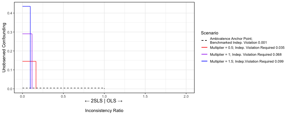
(a) $c_{I}=c_{7}=0$ (no violation); True IR = 0

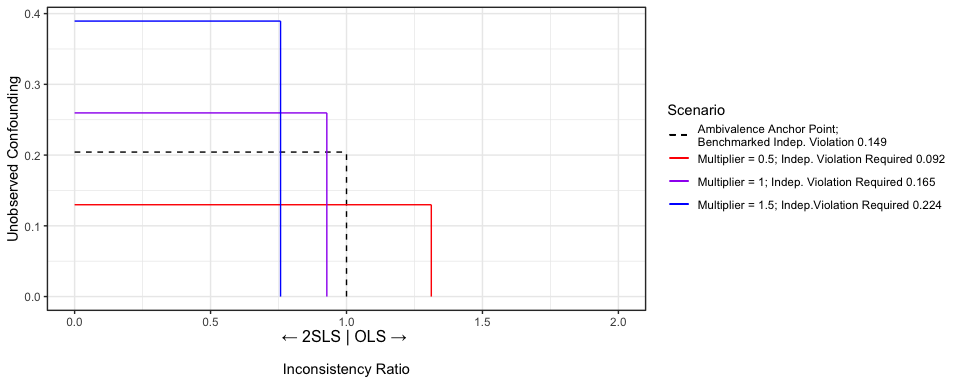
(b) $c_{I}=c_{7}=0.4$; True IR = 0.98

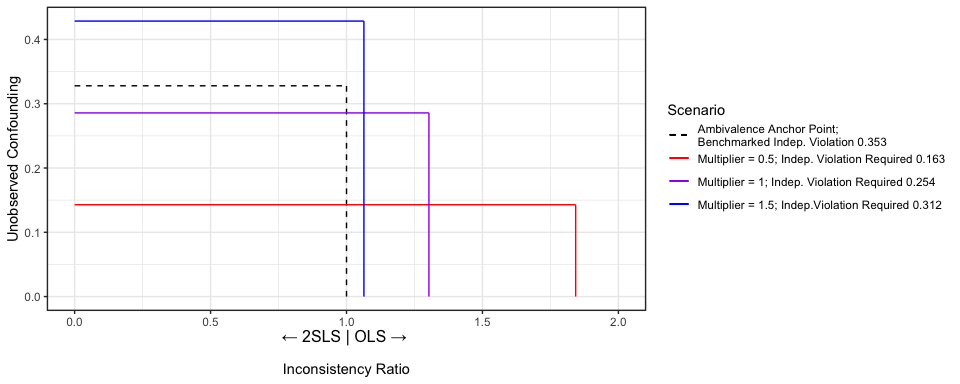
(c) $c_{I}=c_{7}=0.6$; True IR = 1.45

5.3 Treatment Effect Heterogeneity

For the case with no covariates, we set the following structural parameters $\beta_{1}=0.1$, $\beta_{2}=0.2$, $\beta_{3}=0.1$, $\alpha_{1}=0.45$, $\alpha_{2}=0.15$, and $\alpha_{3}=0.1$. For the case with covariates, we have $\beta_{1}=0.1$, $\beta_{2}=0.2$, $\beta_{3}=0.1$, $\beta_{4}$, $\beta_{5}$, $\alpha_{1}=0.45$, $\alpha_{2}=0.15$, $\alpha_{3}=0.1$, $\alpha_{4}=0.15$, and $\alpha_{5}=0.1$. The results are presented in Table 7.

Table 7: Theoretical and Simulated Results for Treatment Effect Heterogeneity

		Method
		OLS without Z	OLS with Z	2SLS with Z
Without covariates	Closed Form Result	0.039	0.044	0.022
	Simulated Result	0.039	0.044	0.021
With covariates	Closed Form Result	0.040	0.037	0.021
	Simulated Result	0.039	0.046	0.021

Figure 14 reflects the how, with increasing treatment effect heterogeneity related to the IV, 2SLS could become more inconsistent than OLS. The structural parameters are the same as the above except that $\alpha_{2}=\alpha_{3}=0.2$.

Figure 14: Heterogeneity Violation Sensitivity Analysis Results with Benchmarking

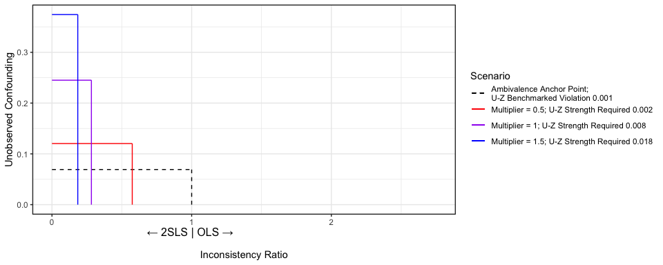
(a) $\alpha_{3}=0$ (no violation); True IR = 0

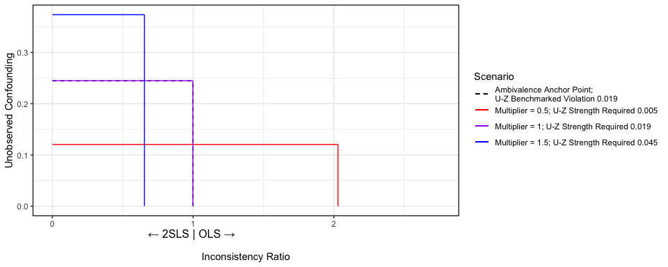
(b) $\alpha_{3}=0.2$; True IR = 1

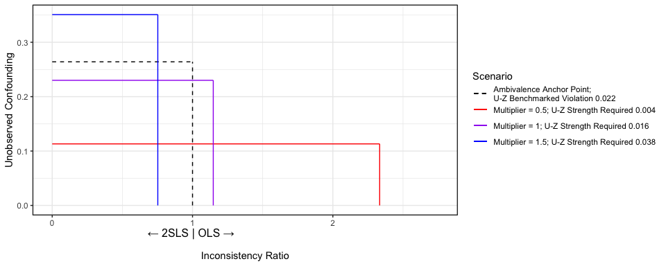
(c) $\alpha_{3}=0.3$; True IR = 1.25

6 Applied Example

We demonstrate the application of our sensitivity analysis in studying neonatal outcomes as a function impacts to the mother during pregnancy. Specifically, we seek to measure the impact of perceived maternal stress during the pregnancy, as measured by the perceived stress scale (PSS),[19] on the birthweight of the neonate (in pounds). The PSS asks the participant several questions related to different symptoms of stress in her life where, in each item, they give a response from zero (almost never) to four (very often) on the Likert scale. Higher scores indicated a larger degree of stress and we treat the overall PSS score as continuous for the purposes of our analysis. From the literature, our hypothesis is that higher stress would lead to lower birthweights;[20] however, due to the observational nature of such data, we are concerned about unmeasured confounding. That is, there may be uobserved factors that affect both perceived maternal stress during pregnancy and birthweight. Therefore, we are motivated to use IVs to isolate the causal effect.

We study 147 mother-child dyads from ecological momentary assessment data collected at at University of California, Irvine. More details regarding the cohort inclusion-exclusion criteria and characteristics can be found in Lazarides et al.[21] For our purposes, at three points during their pregnancy (early, mid, and late), the mothers were asked to fill out a questionnaire on their mobile devices about regarding their stress at ten times throughout the day. Furthermore, each mother repeated the questionnaire for four consecutive days, two of these days being weekends. For each trimester, day, and timepoint, we calculate the current PSS and then calculate the median PSS for that day, which is our exposure of interest for perceived stress. For example, a mother would fill out the questionnaire ten times during Thursday, Friday, Saturday, and Sunday. At each timepoint, we would calculate the PSS and subsequently have four median PSS measurements for each day the data was collected. For the purposes of the application of our sensitivity analysis tool, we only focus on data from the second collection point (i.e. mid-pregnancy).

A potential IV that we utilized was a binary indicator of whether the stress measurements were collected on a weekday or a weekend with the hypothesis being that stress is generally increased on weekdays compared to weekends. Because we had data for both weekdays and weekends, for each mother, we randomly sampled a single day to use as her stress measurement and recorded if this day was a weekday or weekend. This represents a realistic sampling scheme where the mothers may be asked only once to fill the questionnaire and they are randomized to a weekday or weekend. Regressing median PSS upon the weekday indicator IV corroborated our hypothesized relevance and found that weekdays were associated with 0.213 higher points, on average, compared to weekdays (95% CI: [0.038,0.388],$p=0.017$). Nevertheless, the IV was fairly weak with the first-stage $F=5.775$.

For the confounders we adjusted for in both OLS and 2SLS, we utilized the neonate’s sex, the mother’s age, how many previous children the mother has had (i.e. parity), and an indicator for obstetric risk, which summarizes many factors that may result in adverse pregnancy outcomes such as low birth weight. OLS found an insignificant positive relationship where as median stress increased by one, on average, birthweight increased by 0.05 pounds (95% CI: [-0.212,0.313],$p=0.702$). 2SLS found an insignificant relationship but of the opposite sign where a one point increase in median PSS was associated with an 0.19 pound decrease in average birthweight (95% CI: [-2.587, 2.193], $p=0.87$).

The demonstration of our approach is presented in Figure 15. All variables were standardized before inputting it into our tool and, to form the general confounder $W$, the confounders were combined using the first principal component. We may first look at the benchmarks of each assumption violation, which appear to be quite small. Even so, the benchmarked strength of unobserved confounding is relatively small, which overall, in conjunction with the weakness of the IV, leads us to empirically prefer using OLS rather than 2SLS.

Examining each assumption violation individually, if one believes the unobserved confounding is double the observed confounding (the blue line), we are in ambivalence with respect to the exclusion restriction violation but not the independence assumption. Theoretically, there may not be a basis for the weekday indicator to violate the IV assumptions and this is a factor the analyst should weigh against the observed evidence. If the analyst decides to use the IV, there may be concern that, due to exposure effect heterogeneity, the LACE will be far from the ACE. In this specific example, we would be concerned that there is an unobserved covariate that modifies the relationship between median PSS and birthweight in addition to modifying the effect of the weekday indicator on median PSS. Fortunately, the corresponding plot in Figure 15 shows that benchmarked heterogeneity related to the IV is low and will not cause large inconsistency in comparison to benchmarked unobserved confounding (unless we assign a multiplier of $0.5$). Note that we only have one plot for treatment effect heterogeneity because both cases related to the signs yield similar plots and conclusions.

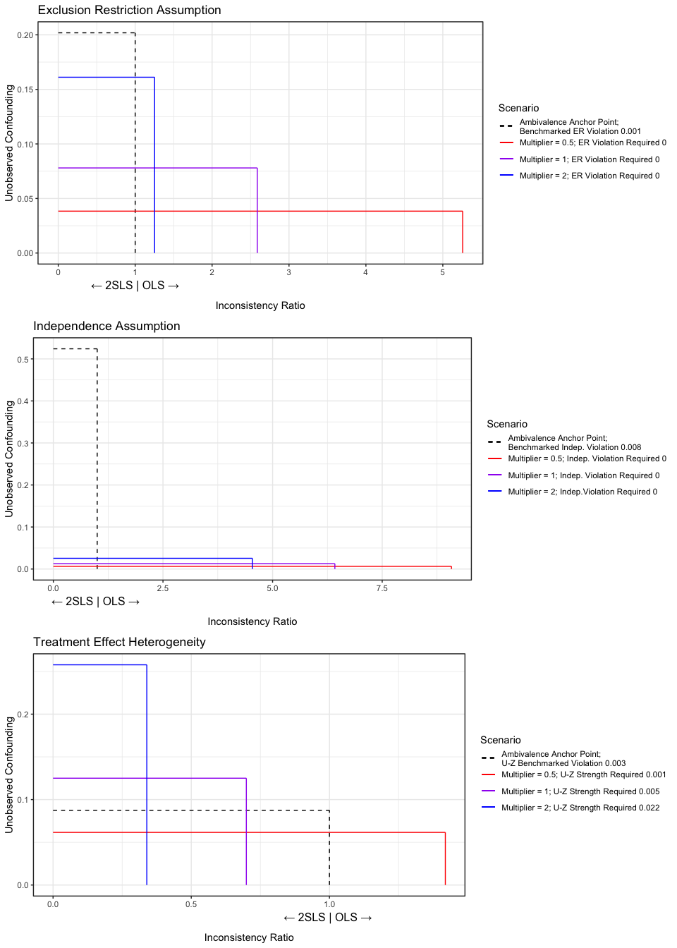
Figure 15: Examining the Three Assumptions for the Weekday Indicator IV

7 Discussion

In this paper, we have investigated two predominant ways that analysts may isolate causal effects: confounders, or the CAC, and via IV, or the IVAC. Furthermore, we have based our study on the notion that each approach may work imperfectly due to assumption violation as is most plausible in the vast majority of real world settings. Our closed-form results that capture interpretable rules of thumb based on DAG edge weights and coefficients, as well as our sensitivity analysis procedure, help guide analysts towards a practical philosophy on how one may execute observational studies. If the goal is to obtain an estimate of the ACE and there is a set of tools that one must choose from, such as the CAC and IVAC, one must ask: when is one tool more advantageous than the other? We have ultimately broken down this question by juxtaposing the degree of unobserved confounding to the degree IV assumption violation, shifting away from perfectionism and providing results for analysts to offer evidence that the estimate computed was the least inconsistent it could have been given the scenario.

Our results show that properly defining confounders and IVs in the study paradigm is only a starting point. Whether a variable will be used in CAC or as an IV in IVAC is not necessarily congruent with its formal definition. In fact, we have presented analytically that, relative to OLS, there are scenarios where a variable should be used as an IV even though it does not meet the strict definition of an IV. For example, in an exclusion restriction violation the variable used as an IV is, by definition, a confounder and, although such a variable is not a "perfect IV," the relative performance of 2SLS would be better than that of OLS. Our sensitivity analysis procedure assists in detecting this by using the observed data.

Another relevant scenario lies in the fact that even though we may have a valid IV, the LACE estimand from 2SLS may be further away from the ACE than an estimand from OLS that is impacted by unobserved confounding. Through our closed form results and sensitivity analysis, we allow an analyst to judge how large heterogeneity would need to be in order for this to occur. Whether the resulting IV estimand remains scientifically useful is a subject of debate that we will not discuss here.[22] Rather, we are interested in directly targeting the ACE and will assume that treatment effect heterogeneity may provide a barrier to this goal. In this sense, the results from our paper may provide case-by-case evidence for and against those who may argue IV analyses may still be useful for the ACE.

Moving to the use of our sensitivity analysis tools, we essentially provide three separate plots for three distinct assumption violation scenarios. If all three plots all agree that either 2SLS is superior or OLS is superior then the suggested approach is clear to the analyst as was largely the case with the birthweight example. However, one may encounter a scenario that the graphs disagree: for example, the exclusion restriction and independence show 2SLS is superior while the treatment effect heterogeneity graph does not. In this case, one should rank the importance of each assumption and consider the observed benchmarks for each assumption violation. Using the multipliers provided or inputting a custom multiplier, one could consider the degree of unobserved confounding across the board in order for all three graphs to agree and evaluate whether these findings are reasonable in the particular study scenario. Similarly, one may further use the implied assumption violations in the legend relative to the benchmarked assumption violations for these purposes. Ultimately, sensitivity analyses are matters of judgement and we aim to provide quantitative tools for analysts to navigate these scenarios.

The results in this paper also have implications on more sophisticated, data-driven variable selection techniques. Users of CAC often will opt to capture confounding by adjusting for the propensity score (PS) using the fitted values of the exposure regressed on the confounders. In order to reduce Type I error, one would model the PS away from the outcome and, thus, it appears reasonable to use penalization or machine learning (ML) techniques to optimize prediction error. There are two main issues with this automated procedure: (1) strong though imperfect IVs would be selected leading to possible bias amplification and (2) omitted variable bias may occur due to shrinkage to zero of important confounders. These points have been mentioned by others[5, 3, 23] and our results further provide analysts information to act in the face of such issues. We may use our results to quantify how strong the confounder or IV should be in order to avoid adjustment altogether or, instead, use it in 2SLS. Future directions may include extending the framework developed in this paper to techniques such as augmented inverse probability of treatment weighting (AIPTW), post-LASSO (PL), targeted minimum loss estimation (TMLE), and double machine learning (DML) to weigh the approaches against one another.[24, 25, 26]

There are several avenues for future research. Firstly, in this paper, we focus only on consistency but in estimation, we may also want to know whether CAC may more efficient than IVAC or vice-versa. Furthermore, if the confidence intervals overlap on the point estimate, which would cause ambivalence. We may additionally wish to move beyond the setting with a continuous exposure and outcome. Nevertheless, if one believes linear probability models (LPMs) are appropriate for the study’s context, then one may extend our results to a binary exposure and outcome. It has been shown that if the probabilities produced by the LPM are not outside of the range of $[0,1]$, or that the probabilities of exposure or outcome are not extreme in the population, then OLS and 2SLS may still give consistent results.[27, 28] For the sensitivity analysis procedure, the results are only as useful as variables available and chosen for benchmarking, which is partially mitigated by using the multipliers. Certainly, other benchmarking quantities for the unobserved quantities than the ones we chose could be used. The aggregation of the covariates into one general confounder $W$ could be done via other methods besides PCA, which is limited when there are categorical variables. Using non-continuous variables also is limited when capturing associations using $R^{2}$ due to the Frechet bounds on the correlation between non-continuous variables being potentially far narrower than $[-1,1]$.[29]

Isolating causal effects in observational data presents many challenges, which foremost include the effect of unobserved confounding. The CAC and IVAC offer potential avenues to mitigate this confounding. Even so, under untestable assumptions, choosing the optimal approach for the problem at hand involves much conjecture. Our closed-form findings and sensitivity analysis approach helps analysts quantitatively justify the approach that they ultimately believe produces an estimate closest to the ACE. The upshot is that, with the information we provide, results from observational studies will both be more transparent and more useful in their interpretation.

8 Acknowledgements

RSZ and DLG are supported by NIH/NIA P30AG066519 and NIH/NIA 1RF1AG075107.

9 Bibliography

10 Appendix

10.1 Proof for the Consistency $\hat{A}_{4}$ under Figure 1

Proof.

We begin by defining following system of structural equations under Figure 1 where $E[\epsilon_{1}|U,Z]=0$ and $E[\epsilon_{2}|X,U]=0$.

$$X=\alpha_{1}U+\alpha_{2}Z+\epsilon_{1}$$ (44)

$$Y=\beta_{1}X+\beta_{2}U+\epsilon_{2}$$ (45)

By the standard definition of the IV estimator, $\hat{A}_{4}=\frac{\widehat{Cov}(Y,Z)}{\widehat{Cov}(X,Z)}$. Where $n$ is the sample size, by finite variance and Slutsky’s theorem we can write:

$$\frac{\widehat{Cov}(Y,Z)}{\widehat{Cov}(X,Z)} =\frac{n^{-1}\sum_{i=1}^{n}y_{i}z_{i}}{n^{-1}\sum_{i=1}^{n}x_{i}z_{i}}\overset{p}{\to}\frac{E[YZ]}{E[XZ]}=\frac{Cov(Y,Z)}{Cov(X,Z)}$$ (46)

Clearly, $Cov(X,Z)=\alpha_{2}=c_{3}$ because $Z\perp\!\!\!\!\perp U$. Moving onto $Cov(Y,Z)$ we write:

$$E[Y|z] =\sum_{u}E[Y|z,u]P(u|z)$$ (47)

$$=\sum_{u}[c_{0}c_{3}z+c_{2}u]P(u)$$ (48)

$$=c_{0}c_{3}z\sum_{u}u+c_{2}\sum_{u}uP(u)$$ (49)

$$=c_{0}c_{3}z$$ (50)

∎

10.2 Proof for Proposition 3.1

Proof.

Using an equivalent definition of the IV estimator, $\hat{A}_{4}=(Z^{T}X)^{-1}(Z^{T}Y)$ we can substitute 9 for $Y$

$$(Z^{T}X)^{-1}(Z^{T}Y) =(Z^{T}X)^{-1}(Z^{T}(c_{0}X+c_{2}U+c_{ER}Z+\epsilon_{3}))$$ (51)

$$=c_{0}+c_{2}(Z^{T}X)^{-1}Z^{T}U+c_{ER}(Z^{T}X)^{-1}Z^{T}Z+(Z^{T}X)^{-1}Z^{T}\epsilon_{3}$$ (52)

$$=c_{0}+c_{2}\frac{n^{-1}\sum_{i=1}^{n}z_{i}u_{i}}{n^{-1}\sum_{i=1}^{n}z_{i}x_{i}}+c_{ER}\frac{n^{-1}\sum_{i=1}^{n}z_{i}^{2}}{n^{-1}\sum_{i=1}^{n}z_{i}x_{i}}+\frac{n^{-1}\sum_{i=1}^{n}\epsilon_{3i}x_{i}}{n^{-1}\sum_{i=1}^{n}z_{i}x_{i}}$$ (53)

$$\overset{p}{\to}c_{0}+c_{2}\frac{Cov(Z,U)}{Cov(Z,X)}+c_{ER}\frac{Var(Z)}{Cov(Z,X)}+\frac{Cov(Z,\epsilon_{3})}{Cov(Z,X}$$ (54)

$$=c_{0}+\frac{c_{ER}}{c_{3}} Z\perp\!\!\!\!\perp U Cov(X,Z)=c_{3}$$ ( and ) (55)

The last line follows from the fact that $Z\perp\!\!\!\!\perp U$ and $E[\epsilon_{3}Z]=0$ by iterated expectation. ∎

10.3 Proofs for Proposition 3.2

10.3.1 Proof for the Consistency of $\hat{A}_{3}$

Proof.

We need to find the value of $\frac{\partial}{\partial x}E[Y|x,z]=c_{0}+c_{2}\frac{\partial}{\partial x}E[U|x,z]$. We will use the FWL theorem to find $\frac{\partial}{\partial x}E[U|x,z]$ by orthogonalizing $Z$ and using consistency. Assuming no intercept, we can write the quantity as $\frac{X^{T}M_{Z}U}{X^{T}M_{Z}X}$ where $M_{Z}=I-Z^{T}(Z^{T}Z)^{-1}Z^{T}$ (residual making matrix). Noting that $Cov(X,Z)=c_{3}+c_{1}c_{I}$ and $Cov(U,Z)=c_{I}$, we have:

$$\frac{X^{T}M_{Z}U}{X^{T}M_{Z}X} =\frac{\sum_{i=1}^{n}[x_{i}-(c_{3}+c_{1}c_{I})z_{i}][u_{i}-c_{I}z_{i}]}{\sum_{i=1}^{n}[x_{i}-(c_{3}+c_{1}c_{I})z_{i}]^{2}} \overset{p}{\to}\frac{Cov[X-(c_{3}+c_{1}c_{I})Z,U-c_{I}Z]}{Var[X-(c_{3}+c_{1}c_{I})Z]}$$ (56)

$$=\frac{c_{1}+c_{3}c_{I}-c_{I}(c_{3}+c_{1}c_{I})}{1-(c_{3}+c_{1}c_{I})^{2}}=\frac{c_{1}(1-c_{I}^{2})}{1-(c_{3}+c_{1}c_{I})^{2}}$$ (57)

∎

10.3.2 Proof for the Consistency of $\hat{A}_{4}$

Proof.

In a similar derivation Proposition 3.1 but plugging in $c_{0}X+c_{2}U+\epsilon_{3}$ for the structural equation of $Y$, we obtain

$$\hat{A}_{4} \overset{p}{\to}c_{0}+c_{2}\frac{Cov(Z,U)}{Cov(Z,X)}+\frac{Cov(Z,\epsilon_{3})}{Cov(Z,X)}$$ (58)

$$=c_{0}+c_{2}\frac{Cov(Z,U)}{Cov(Z,X)}$$ (59)

$$=c_{0}+\frac{c_{2}c_{I}}{c_{3}+c_{1}c_{I}}$$ (60)

Note that the unconditional association between $X$ and $Z$ goes has two paths: the direct path $X\to Z$ and the indirect path $X\leftarrow U\to Z$. ∎

10.4 Proofs for Proposition 3.3

10.4.1 Proof for the consistency of $\hat{A}_{2}$

Proof.

We simply will compute the regression of $Y$ on $X$ where $\hat{A}_{2}\overset{p}{\to}Cov(Y,X)$.

$$Cov(Y,X) =Cov(\beta_{1}X+\beta_{2}U+\beta_{3}XU+\epsilon_{2},X)=\beta_{1}+\beta_{2}\alpha_{2}+\beta_{3}Cov(XU,X)$$ (61)

$$=\beta_{1}+\alpha_{2}\beta_{2}+2\alpha_{1}\alpha_{3}\beta_{3}$$ (62)

Where $Cov(XU,X)=2\alpha_{1}\alpha_{3}$ because

$$Cov(XU,X) =Cov(U(\alpha_{1}Z+\alpha_{2}U+\alpha_{3}ZU+\epsilon_{1}),X)$$ (63)

$$=\alpha_{1}Cov(UZ,X)+\alpha_{2}Cov(U^{2},X)+\alpha_{3}Cov(ZU^{2},X)$$ (64)

$$=\underbrace{\alpha_{1}E[UZX]}_{B_{1}}+\underbrace{\alpha_{2}E[U^{2}X]}_{B_{2}}+\underbrace{\alpha_{3}E[ZU^{2}X]}_{B_{3}}$$ (65)

$B_{1}=\alpha_{1}\alpha_{3}$ because

$$E[XUZ] =E[ZE[XU|Z]]=E[ZE[(\alpha_{1}Z+\alpha_{2}U+\alpha_{3}ZU+\epsilon_{1})U|Z]]$$ (66)

$$=E[Z(\alpha_{1}E[UZ|Z]+\alpha_{2}E[U^{2}|Z]+\alpha_{3}E[ZU^{|}Z]+E[U\epsilon_{1}|Z)]$$ (67)

$$=E[\alpha_{1}Z^{2}E[U]+\alpha_{2}ZE[U^{2}]+\alpha_{3}ZE[U^{2}]+E[U\epsilon_{1}]]$$ (68)

$$=E[\alpha_{2}Z+\alpha_{3}Z^{2}]=\alpha_{3}$$ (69)

$B_{2}=0$ because $E[U^{2}X]=E[U^{2}E[X|U]]=\alpha_{2}E[U^{3}]=0$ because $E[U^{3}]=0$.

$B_{3}=\alpha_{1}\alpha_{3}$ because

$$E[ZU^{2}X] =E[ZU^{2}(\alpha_{1}Z+\alpha_{2}U+\alpha_{3}ZU+\epsilon_{1})]$$ (70)

$$=\alpha_{1}E[Z^{2}U^{2}]+\alpha_{2}E[ZU^{3}]+\alpha_{3}E[Z^{2}U^{3}]$$ (71)

$$=\alpha_{1}$$ (72)

Where the last equality follows because $Z\perp\!\!\!\!\perp U$ and $E[U^{3}]=0$. ∎

10.4.2 Proof for the consistency of $\hat{A}_{3}$

Proof.

Similar to proposition 3.2, we will proceed via FWL to find the value of $A_{3}=\frac{X^{T}M_{Z}Y}{X^{T}M_{Z}X}$. First, we need to find $Cov(Z,X)$ and $Cov(Z,Y)$:

$$Cov(Z,X) =Cov(Z,\alpha_{1}Z+\alpha_{2}U+\alpha_{3}ZU+\epsilon_{1})=\alpha_{1}$$ (73)

and (74)

$$Cov(Z,Y) =Cov(Z,\beta_{1}X+\beta_{2}U+\beta_{X}U+\epsilon_{2})=E[Z(\beta_{1}X+\beta_{2}U+\beta_{X}U+\epsilon_{2})]$$ (75)

$$=E[\beta_{1}XZ+\beta_{2}UZ+\beta_{3}XUZ+Z\epsilon_{2}]=\alpha_{1}\beta_{1}+\alpha_{3}\beta_{3}$$ (76)

Going back to FWL, letting $\lambda=\alpha_{1}\beta_{1}+\alpha_{3}\beta_{3}$, we now have

$$\frac{X^{T}M_{Z}Y}{X^{T}M_{Z}X} =\frac{(X-\alpha_{1}Z)^{T}(Y-\lambda Z)}{(X-\alpha_{1}Z)^{T}(X-\alpha_{1}Z)}=\frac{\sum_{i=1}^{n}X_{i}Y_{i}-\lambda X_{i}Z_{i}-\alpha_{1}Z_{i}Y_{i}+\alpha_{1}\lambda Z_{i}^{2}}{\sum_{i=1}^{n}(X_{i}-\alpha_{1}Z_{i})^{2}}$$ (77)

$$\overset{p}{\to}\frac{E[X_{i}Y_{i}-\lambda X_{i}Z_{i}-\alpha_{1}Z_{i}Y_{i}+\alpha_{1}\lambda Z^{2}]}{E[(X_{i}-\alpha_{1}Z_{i})^{2}]}$$ (78)

$$=\frac{Cov(X,Y)-\lambda Cov(X,Z)-\alpha_{1}Cov(Z,Y)+\alpha_{1}\lambda Var(X)}{1-\alpha_{1}^{2}}$$ (79)

$$=\frac{(\beta_{1}+\alpha_{2}\beta_{2}+2\alpha_{1}\alpha_{3}\beta_{3})-\lambda\alpha_{1}-\alpha_{1}\lambda+\alpha_{1}\lambda}{1-\alpha_{1}^{2}}$$ (80)

$$=\frac{\beta_{1}+\alpha_{2}\beta_{2}+2\alpha_{1}\alpha_{3}\beta_{3}-\alpha_{1}^{2}\beta_{1}+\alpha_{3}\beta_{3}\alpha_{1}}{1-\alpha_{1}^{2}}=\beta_{1}+\frac{\alpha_{2}\beta_{2}+\alpha_{1}\alpha_{3}\beta_{3}}{1-\alpha_{1}^{2}}$$ (81)

∎

10.4.3 Proof for the consistency of $\hat{A}_{4}$

Proof.

We can compute the Wald estimator from the quantities computed in the proof for $\hat{A}_{3}$. In particular, $Cov(Z,Y)$ and $Cov(Z,X)$.

$$\hat{A}_{4} \overset{p}{\to}\frac{Cov(Z,Y)}{Cov(Z,X)}=\frac{\alpha_{1}\beta_{1}+\alpha_{3}\beta_{3}}{\alpha_{1}}=\beta_{1}+\frac{\alpha_{3}\beta_{3}}{\alpha_{1}}$$ (82)

∎

10.5 Proofs for Proposition 3.5

10.5.1 Proof for the consistency of $\hat{A}_{2}$

Proof.

Our goal is to find $\frac{\partial}{\partial x}E[Y|x,w]$, which, by FWL, is equivalent to the convergence in probability of $\frac{X^{T}M_{W}Y}{X^{T}M_{W}X}$. Because we have already demonstrated the use of FWL, we will skip several intermediate steps. Letting $\eta=c_{6}+c_{5}c_{0}$

$$\frac{X^{T}M_{W}Y}{X^{T}M_{W}X} =\frac{(X-c_{5}W)^{T}(Y-\eta W}{((X-c_{5}W))}\overset{p}{\to}\frac{Cov(X,Y)-\eta Cov(W,Y)+c_{5}\eta}{1-c_{5}^{2}}$$ (83)

$$=\frac{c_{0}+c_{1}c_{2}+c_{2}c_{3}c_{I}-\eta c_{5}-\eta c_{5}+c_{5}\eta)}{1-c_{5}^{2}}=c_{0}+\frac{c_{1}c_{2}+c_{2}c_{3}c_{I}}{1-c_{5}^{2}}$$ (84)

∎

10.5.2 Proof for the consistency of $\hat{A}_{3}$

Proof.

Our goal is to find $\frac{\partial}{\partial x}E[Y|x,w,z]$, which, by FWL, is equivalent to the limit of $\frac{X^{T}M_{\mathbb{B}}Y}{X^{T}M_{\mathbb{B}}X}$ where $\mathbb{B}=[W,Z]$ or the residuals of regressing both $W$ and $Z$. To simplify matters, we can expand $Y$

$$\frac{X^{T}M_{\mathbb{B}}Y}{X^{T}M_{\mathbb{B}}X} =\frac{X^{T}M_{\mathbb{B}}(c_{0}+c_{2}U+c_{6}W+\epsilon_{2})}{X^{T}M_{\mathbb{B}}X}$$ (85)

$$=c_{0}+c_{2}\frac{X^{T}M_{\mathbb{B}}U}{X^{T}M_{\mathbb{B}}X}$$ (86)

Where the last line follows from the orthogonality of $\epsilon_{2}$ and the result of $W$ being regressed upon itself being that the residuals are $0$. So we are focused on two regressions: $E[X|w,z]=\gamma_{1}W+\gamma_{2}Z$ and $E[U|w,z]=\pi_{1}W+\pi_{2}Z$. Using FWL, we find the value of the coefficients to be

$$\gamma_{1} =\frac{W^{T}M_{Z}X}{W^{T}M_{Z}W}\overset{p}{\to}c_{5}-\frac{c_{1}c_{I}c_{7}}{1-c_{7}^{2}},$$ (87)

$$\gamma_{2} =\frac{Z^{T}M_{W}X}{Z^{T}M_{W}Z}\overset{p}{\to}c_{3}+\frac{c_{1}c_{I}}{1-c_{7}^{2}},$$ (88)

$$\pi_{1} =\frac{W^{T}M_{Z}U}{W^{T}M_{Z}W}\overset{p}{\to}\frac{-c_{I}c_{7}}{1-c_{7}^{2}},$$ (89)

$$\pi_{2} =\frac{Z^{T}M_{W}U}{Z^{T}M_{W}Z}\overset{p}{\to}\frac{c_{I}}{1-c_{7}^{2}}$$ (90)

Putting this altogether, we write $A_{3}=c_{0}+c_{2}\frac{Cov(X-\gamma_{1}W-\gamma_{2}Z,U-\pi_{1}W-\pi_{2}Z)}{Var(X-\gamma_{1}W-\gamma_{2}Z)}$ (note that we are now in the limit). Expanding the numerator we get

$$c_{2} \bigg{[}Cov(X,U)-\pi_{1}Cov(X,W)-\pi_{2}Cov(X,Z)-\gamma_{1}Cov(W,U)+\gamma_{1}\pi_{1}$$ (91)

$$+\gamma_{1}\pi_{2}Cov(W,Z)-\gamma_{2}Cov(Z,U)+\gamma_{2}\pi_{1}Cov(W,Z)+\gamma_{2}\pi_{2}\bigg{]}$$ (92)

Noting that $Cov(X,U)=c_{1}+c_{3}c_{I}$, $Cov(X,W)=c_{5}+c_{3}c_{7}$, $Cov(X,Z)=c_{3}+c_{1}c_{I}+c_{5}c_{7}$, $Cov(W,U)=0$, $Cov(W,Z)=c_{7}$, and $Cov(Z,U)=c_{I}$, we can simplify the above expression to

$$c_{1}c_{2}+\frac{c_{1}c_{2}c_{I}^{2}c_{7}}{1-c_{7}^{2}}-\frac{c_{1}c_{2}c_{I}^{2}c_{7}}{(1-c_{7}^{2})^{2}}+\frac{c_{1}c_{2}c_{I}c_{7}^{3}}{(1-c_{7}^{2})^{2}}-\frac{c_{1}c_{2}c_{I}^{2}}{1-c_{7}^{2}}$$ (93)

$$=c_{1}c_{2}+\frac{c_{1}c_{2}c_{I}^{2}c_{7}-c_{1}c_{2}c_{I}^{2}}{1-c_{7}^{2}}+\frac{c_{1}c_{2}c_{I}^{2}c_{7}(c_{7}^{2}-1}{(1-c_{7}^{2})^{2}}=c_{1}c_{2}+\frac{c_{1}c_{2}c_{I}^{2}c_{7}-c_{1}c_{2}c_{I}^{2}-c_{1}c_{2}c_{I}^{2}c_{7}}{1-c_{7}^{2}}$$ (94)

$$=c_{1}c_{2}-\frac{c_{1}c_{2}c_{I}^{2}}{1-c_{7}^{2}}$$ (95)

For the denominator

$$Var(X-\gamma_{1}W-\gamma_{2}Z) =1+\gamma_{1}^{2}+\gamma_{2}^{2}-2\gamma_{1}Cov(X,W)-2\gamma_{2}Cov(X,Z)+2\gamma_{1}\gamma_{2}Cov(W,Z)$$ (96)

After combining like terms we obtain

$$1-c_{5}^{2}-c_{3}^{2}+\frac{c_{1}^{2}c_{I}^{2}}{(1-c_{7}^{2})^{2}}-2c_{3}c_{5}c_{7}-2c_{1}c_{3}c_{I}-2\frac{c_{1}^{2}c_{I}^{2}}{1-c_{7}^{2}}-\frac{c_{1}^{2}c_{I}^{2}c_{7}^{2}}{(1-c_{7}^{2})^{2}}$$ (98)

$$=1-c_{5}^{2}-c_{3}^{2}-2c_{3}c_{5}c_{7}-2c_{1}c_{3}c_{I}-\frac{c_{1}^{2}c_{I}^{2}}{1-c_{7}^{2}}+[c_{3}^{2}c_{7}^{2}-c_{3}^{2}c_{7}^{2}]$$ (99)

$$=1-(c_{5}+c_{3}c_{7})^{2}+c_{3}^{2}c_{7}^{2}-c_{3}^{2}-2c_{1}c_{3}c_{I}-\frac{c_{1}^{2}c_{I}^{2}}{1-c_{7}^{2}}$$ (100)

$$=1-(c_{5}+c_{3}c_{7})^{2}-(1-c_{7}^{2})(c_{3}^{2}+\frac{2c_{1}c_{3}c_{I}}{1-c_{7}^{2}}+\frac{c_{1}^{2}c_{I}^{2}}{1-c_{7}^{2}})$$ (101)

$$=1-(c_{5}+c_{3}c_{7})^{2}-(1-c_{7}^{2})(c_{3}+\frac{c_{1}c_{I}}{1-c_{7}^{2}})^{2}$$ (102)

∎

10.5.3 Proof for the consistency of $\hat{A}_{4}$

Proof.

Via FWL, $\frac{\frac{\partial}{\partial z}E[Y|z,w]}{\frac{\partial}{\partial z}E[X|z,w]}=\frac{}{}=\frac{Z^{T}M_{W}Y}{Z^{T}M_{W}X}$. Re-using quantities from the proof for $A_{3}$ and, additionally $Cov(Z,Y)=c_{0}c_{3}+c_{2}c_{I}+c_{6}c_{7}+c_{0}c_{5}c_{7}+c_{0}c_{1}c_{I}$ and $Cov(Y,W)=c_{0}c_{5}+c_{6}+c_{0}c_{3}c_{7}$ we have

$$\frac{Z^{T}M_{W}Y}{Z^{T}M_{W}X} \overset{p}{\to}\frac{Cov(Z,Y)-Cov(Z,W)Cov(Y,W)}{Cov(X,Z)-Cov(Z,W)Cov(X,W)}$$ (103)

$$=\frac{c_{0}c_{3}+c_{2}c_{I}+c_{6}c_{7}+c_{0}c_{5}c_{7}+c_{0}c_{1}c_{I}-c7(c_{0}c_{5}+c_{6}+c_{0}c_{3}c_{7})}{c_{3}+c_{1}c_{I}+c_{5}c_{7}-c_{7}(c_{5}+c_{3}c_{7})}$$ (104)

$$=\frac{c_{0}(c_{3}+c_{1}c_{I}-c_{7}^{2}c_{3})+c_{2}c_{I}}{c_{3}+c_{1}c_{I}-c_{7}^{2}c_{3}}=\frac{c_{2}c_{I}}{c_{3}(1-c_{7}^{2})+c_{1}c_{I}}$$ (105)

∎

10.6 Proof for Proposition 3.6

10.6.1 Results for $A_{2}$

Proof.

Our goal is to find the value of $\frac{\partial}{\partial x}\frac{X^{T}M_{\mathbb{C}}Y}{X^{T}M_{\mathbb{C}}X}$ where $\mathbb{C}=[W,XW]$. Because $Cov(W,XW)=0$, we can write the following linear conditional expectations

$$E[X|W,XW]=Cov(X,W)W+\frac{Cov(X,XW)}{Var(XW)}XW=\alpha_{4}W+\frac{2\alpha_{1}\alpha_{5}}{\alpha_{4}^{2}+2\alpha_{5}^{2}+1}XW,$$ (106)

$$E[Y|W,XW]=Cov(Y,W)W+\frac{Cov(Y,XW)}{Var(XW)}XW=(\beta_{1}\alpha_{4}+\beta_{4})W+\frac{2\alpha_{1}\alpha_{5}\beta_{1}+\beta_{5}(\alpha_{4}^{2}+2\alpha_{5}^{2}+1)}{\alpha_{4}^{2}+2\alpha_{5}^{2}+1}XW.$$ (107)

Returning back to the FWL expression, we now plug in the above conditional expectations. Focusing on the numerator, which is rewritten as $Cov(X-E[X|W,XW],Y-E[X|W,XW])$, we have

$$Cov(X-\alpha_{4}W-\frac{2\alpha_{1}\alpha_{5}}{\alpha_{4}^{2}+2\alpha_{5}^{2}+1}XW,Y-\beta_{1}\alpha_{4}+\beta_{4}W-\frac{2\alpha_{1}\alpha_{5}\beta_{1}+\beta_{5}(\alpha_{4}^{2}+2\alpha_{5}^{2}+1)}{\alpha_{4}^{2}+2\alpha_{5}^{2}+1}XW$$ (108)

$$=Cov(X,Y)-\frac{\frac{2\alpha_{1}\alpha_{5}\beta_{1}+\beta_{5}(\alpha_{4}^{2}+2\alpha_{5}^{2}+1)}{\alpha_{4}^{2}+2\alpha_{5}^{2}+1}Cov(X,XW)}{\alpha_{4}^{2}+2\alpha_{5}^{2}+1}-\alpha_{4}Cov(W,Y)-$$ (109)

$$\frac{2\alpha_{4}\alpha_{5}Cov(XW,Y)}{\alpha_{4}^{2}+2\alpha_{5}^{2}+1}+\frac{\frac{2\alpha_{1}\alpha_{5}\beta_{1}+\beta_{5}(\alpha_{4}^{2}+2\alpha_{5}^{2}+1)}{\alpha_{4}^{2}+2\alpha_{5}^{2}+1}2\alpha_{1}\alpha_{5}}{\alpha_{4}^{2}+2\alpha_{5}^{2}+1}$$ (110)

$$=\beta_{1}+\beta_{2}\alpha_{2}+2\alpha_{1}\alpha_{3}\beta_{3}+\beta_{4}\alpha_{4}+2\alpha_{1}\alpha_{5}\beta_{5}-\alpha_{4}(\beta_{1}\alpha_{4}+\beta_{4})-\frac{2\alpha_{1}\alpha_{5}\frac{2\alpha_{1}\alpha_{5}\beta_{1}+\beta_{5}(\alpha_{4}^{2}+2\alpha_{5}^{2}+1)}{\alpha_{4}^{2}+2\alpha_{5}^{2}+1}}{\alpha_{4}^{2}+2\alpha_{5}^{2}+1}$$ (111)

$$=\beta_{1}+\beta_{2}\alpha_{2}+2\alpha_{1}\alpha_{3}\beta_{3}-\alpha_{4}^{2}\beta_{1}-\frac{4\alpha_{1}^{2}\alpha_{5}^{2}\beta_{1}}{\alpha_{4}^{2}+2\alpha_{5}^{2}+1}.$$ (112)

Focusing on the denominator:

$$Var(X-\alpha_{4}W-\frac{2\alpha_{1}\alpha_{5}}{\alpha_{4}^{2}+2\alpha_{5}^{2}+1}XW)=1+\alpha^{4}+\frac{4\alpha_{1}^{2}\alpha_{5}^{2}}{\alpha_{4}^{2}+2\alpha_{5}^{2}+1}-2\alpha_{4}^{2}-\frac{8\alpha_{1}^{2}\alpha_{5}^{2}}{\alpha_{4}^{2}+2\alpha_{5}^{2}+1}$$ (113)

$$=1-\alpha_{4}-\frac{4\alpha_{1}^{2}\alpha_{5}^{2}}{\alpha_{4}^{2}+2\alpha_{5}^{2}+1}.$$ (114)

Thus, we obtain the final result $\beta_{1}+\frac{\beta_{2}\alpha_{2}+2\alpha_{1}\alpha_{3}\beta_{3}}{1-\alpha_{4}-\frac{4\alpha_{1}^{2}\alpha_{5}^{2}}{\alpha_{4}^{2}+2\alpha_{5}^{2}+1}}$. ∎

10.6.2 Results for $A_{4}$

Due to there being two endogenous variables, $X$ and $XW$, we will need to utilize two instruments, which are $Z$ and $ZW$, respectively. We will have the following series of linear conditional expectations, noting that $Cov(XW,W)=0$

$$E[X|W,Z,ZW]=Cov(X,W)W+Cov(Z,X)Z+Cov(ZW,X)ZW,$$ (115)

$$E[XW|Z,ZW]=Cov(XW,Z)Z+Cov(XW,ZW)ZW,$$ (116)

$$E[Y|\hat{X},\hat{XW},W]=\frac{Cov(Y,\hat{X})}{Var(\hat{X})}\hat{X}+\frac{Cov(Y,\hat{XW})}{Var(\hat{XW})}\hat{XW}+Cov(Y,W)W$$ (117)

where $\hat{X}$ and $\hat{XW}$ are the fitted values from the $E[X|W,Z,ZW]$ and $E[XW|Z,ZW]$, respectively. The coefficient of interest from 2SLS is thus $\frac{Cov(Y,\hat{X})}{Var(\hat{X})}$ or, returning to FWL, denoted as $\frac{\partial}{\partial\hat{x}}\frac{\hat{X}M_{\mathbb{D}}Y}{\hat{X}M_{\mathbb{D}}\hat{X}}$ where $\mathbb{D}=[W,\hat{XW}]$.

First, we will write out the relevant covariances and variances:

$$Cov(W,\hat{X}) =\alpha_{4}$$ (118)

$$Cov(\hat{XW},\hat{X}) =2\alpha_{1}\alpha_{5}$$ (119)

$$Cov(W,Y) =\beta_{1}\alpha_{4}+\beta_{4}$$ (120)

$$Cov(\hat{XW},Y) =\alpha_{5}\beta_{1}Cov(Z,X)+\alpha_{5}\beta_{3}Cov(Z,XU)+\beta_{5}\alpha_{5}Cov(Z,XW)$$ (121)

$$+\alpha_{1}\beta_{1}Cov(ZW,X)+\alpha_{1}\beta_{3}Cov(ZW,XU)+\alpha_{1}\beta_{5}Cov(ZW,XW)$$ (122)

$$=2\alpha_{1}\alpha_{5}\beta_{1}+\alpha_{3}\alpha_{5}\beta_{3}+\beta_{5}\alpha_{5}^{2}+\alpha_{1}^{2}\beta_{5}$$ (123)

$$Var(\hat{X)} =\alpha_{4}^{2}+\alpha_{1}^{2}+\alpha_{5}^{2}$$ (124)

$$Var(\hat{XW}) =\alpha_{5}^{2}+\alpha_{1}^{2}$$ (125)

$$Cov(\hat{X},Y) =\alpha_{4}Cov(W,Y)+\alpha_{1}Cov(Z,Y)+\alpha_{5}Cov(ZW,Y)$$ (126)

$$=\alpha_{4}(\beta_{1}\alpha_{4}+\beta_{4})+\alpha_{1}(\alpha_{1}\beta_{1}+\alpha_{3}\beta_{3}+\alpha_{5}\beta_{5})+\alpha_{5}(\beta_{1}\alpha_{5}+\beta_{5}\alpha_{1})$$ (127)

$$Cov(ZW,Y)=\beta_{1}\alpha_{5}+\beta_{5}\alpha_{1}$$ (128)

Because $Cov(\hat{XW},W)=0$ we can simply substitute the covariances in the FWL expression as such

$$\frac{Cov(\hat{X}-\alpha_{4}W-\frac{2\alpha_{1}\alpha_{5}}{\alpha^{5}+\alpha_{1}^{2}}\hat{XW},Y-(\beta_{1}\alpha_{4}+\beta_{4})W-Cov(\hat{XW},Y)\hat{XW})}{\hat{X}-\alpha_{4}W-\frac{2\alpha_{1}\alpha_{5}}{\alpha^{5}+\alpha_{1}^{2}}\hat{XW}}$$ (129)

Now focusing on the numerator, can further simplify to

$$Cov(\hat{X},Y)-(\beta_{1}\alpha_{4}+\beta_{4})Cov(\hat{X}W)-\frac{Cov(\hat{XW},Y)}{\alpha_{5}^{2}+\alpha_{1}^{2}}-\frac{2\alpha_{1}\alpha_{5}Cov(\hat{XW},Y)}{\alpha^{5}+\alpha_{1}^{2}}$$ (130)

$$+\frac{2\alpha_{1}\alpha_{5}Cov(\hat{XW},Y)Var(\hat{XW})}{(\alpha^{5}+\alpha_{1}^{2})^{2}}$$ (131)

$$=\alpha_{1}(\alpha_{1}\beta_{1}+\alpha_{3}\beta_{3}+\alpha_{5}\beta_{5})+\alpha_{5}(\beta_{1}\alpha_{5}+\beta_{5}\alpha_{1})-\frac{2\alpha_{1}\alpha_{5}Cov(\hat{XW},Y)}{\alpha^{5}+\alpha_{1}^{2}}$$ (132)

$$=\alpha_{1}\beta_{1}+\alpha_{1}\alpha_{3}\beta_{3}+2\alpha_{1}\alpha_{5}\beta_{5}+\beta_{1}\alpha_{5}^{2}$$ (133)

$$-\frac{4\alpha_{1}\alpha_{5}^{2}\beta_{1}+2\alpha_{1}\alpha_{3}\alpha_{5}^{2}\beta_{3}+2\alpha_{1}\alpha_{5}^{3}\beta_{5}+2\alpha_{1}^{3}\alpha_{5}\beta_{5}}{\alpha_{5}^{2}+\alpha_{1}^{2}}$$ (134)

$$=\beta_{1}\bigg{[}\alpha_{1}^{2}+\alpha_{5}^{2}-\frac{4\alpha_{1}^{2}\alpha_{5}\beta_{1}}{\alpha^{5}+\alpha_{1}^{2}}\bigg{]}+\alpha_{1}\alpha_{3}\beta_{3}-\frac{2\alpha_{1}\alpha_{3}\alpha_{5}^{2}\beta_{3}}{\alpha_{1}^{2}+\alpha_{5}^{2}}.$$ (135)

For the denominator, we have

$$Var(\hat{X}-\alpha_{4}W-\frac{2\alpha_{1}^{2}\alpha_{5}^{2}}{\alpha_{1}^{2}+\alpha_{5}^{2}}\hat{XW}) =\alpha_{4}^{2}+\alpha_{1}^{2}+\alpha_{5}^{2}+\alpha_{4}^{2}+\frac{4\alpha_{1}^{2}\alpha_{5}^{2}}{\alpha_{1}^{2}+\alpha_{5}^{2}}$$ (136)

$$-2\alpha_{4}^{2}-\frac{8\alpha_{1}^{2}\alpha_{5}^{2}}{\alpha_{1}^{2}+\alpha_{5}^{2}}$$ (137)

$$=\alpha_{1}^{2}+\alpha_{5}^{2}-\frac{4\alpha_{1}^{2}\alpha_{5}^{2}}{\alpha_{1}^{2}+\alpha_{5}^{2}}.$$ (138)

Therefore, all together we obtain the final result of

$$\beta_{1}+\frac{\alpha_{1}\alpha_{3}\beta_{3}-\frac{2\alpha_{1}\alpha_{3}\alpha_{5}^{2}\beta_{3}}{\alpha_{1}^{2}+\alpha_{5}^{2}}}{\alpha_{1}^{2}+\alpha_{5}^{2}-\frac{4\alpha_{1}^{2}\alpha_{5}^{2}}{(\alpha_{1}^{2}+\alpha_{5}^{2}})}$$ (139)

10.7 Proof for Exclusion Restriction $R^{2}$ Proposition 4.1

Proof.

We will first rewriting each edge weight as an $R^{2}$ quantities:

$$|c_{1}| =\sqrt{R^{2}_{X\sim U}}$$ (140)

$$|c_{2}| =\frac{Cov(Y^{\perp X,Z,W},U^{\perp X,W,Z})}{Var(U^{\perp X,W,Z})}=\frac{Cor(Y^{\perp X,Z,W},U^{\perp X,W,Z}))sd(Y^{\perp X,W,Z})}{sd(U^{\perp X,W,Z}))}$$ (141)

$$=\sqrt{R^{2}_{Y\sim U|X,W,Z}}\frac{sd(Y^{\perp X,W,Z})}{sd(U^{\perp X,W,Z})}$$ (142)

$$|c_{3}| =\sqrt{R^{2}_{X\sim Z}}$$ (143)

$$|c_{ER}| =\frac{Cov(Y^{\perp X,U,W},Z^{\perp X,U,W})}{Var(Z^{\perp X,U,W})}=\frac{Cor(Y^{\perp X,U,W},Z^{\perp X,U,W})sd(Y^{\perp X,U,W})}{sd(Z^{\perp X,U,W})}$$ (144)

$$=\sqrt{R^{2}_{Y\sim Z|X,U,W}}\frac{sd(Y^{\perp X,U,W})}{sd(Z^{\perp X,U,W})}$$ (145)

$$|c_{5}| =\sqrt{R^{2}_{X\sim W}}$$ (146)

where $\perp$ represents orthogonalizing the variables in the superscript. Because $W\perp\!\!\!\!\perp Z$, $1-c_{3}^{2}-c_{5}^{2}=1-R^{2}_{X\sim W+Z}$. Substituting this into the expression for the trade-off we obtain

$$\frac{\sqrt{R^{2}_{Y\sim Z|X,U,W}}\frac{sd(Y^{\perp X,U,W})}{sd(Z^{\perp X,U,W})}}{\sqrt{R^{2}_{X\sim Z}}}>\frac{\sqrt{R^{2}_{X\sim U}R^{2}_{Y\sim U|X,W,Z}}\frac{sd(Y^{\perp X,W,Z})}{sd(U^{\perp X,W,Z})}}{1-R^{2}_{X\sim W+Z}}$$ (147)

We can further simplify the expression by canceling out like terms and noting that

$$sd(U^{\perp X,W,Z})=\frac{sd(U^{\perp X,W,Z})sd(U^{\perp W,Z})}{sd(U^{\perp W,Z})}=\sqrt{1-R^{2}_{U\sim X|W,Z}}$$ (148)

because $sd(U^{\perp W,Z})=1$ due to $U\perp\mkern-9.5mu\perp Z$ and $U\perp\mkern-9.5mu\perp W$. Thus, our final expression is

$$\frac{\sqrt{R^{2}_{Y\sim Z|X,U,W}}\sqrt{1-R^{2}_{Y\sim U|X,W}}(1-R^{2}_{X\sim W+Z})}{\sqrt{1-R^{2}_{Y\sim Z|X,W}}\sqrt{R^{2}_{X\sim Z}}sd(Z^{\perp X,W})}>\frac{\sqrt{R^{2}_{X\sim U}R^{2}_{Y\sim U|X,W,Z}}}{\sqrt{1-R^{2}_{U\sim X|W,Z}}}$$ (149)

∎

10.8 Proof for Independence $R^{2}$ Proposition 4.2

Proof.

We will first translate the edge weights or the linear combination of the edge weights as $R^{2}$ quantities. Note that $c_{2}$ cancels out in the inequality so we do not need to re-write this quantity.

$$|c_{1}| =\sqrt{R^{2}_{X\sim U|Z,W}}\frac{sd(X^{\perp Z,W})}{sd(U^{\perp Z,W})}$$ (150)

$$|c_{3}| =\sqrt{R^{2}_{X\sim Z|U,W}}\frac{sd(X^{\perp U,W})}{sd(Z^{\perp U,W})}$$ (151)

$$|c_{I}| =\sqrt{R^{2}_{Z\sim U}}$$ (152)

$$|c_{7}| =\sqrt{R^{2}_{Z\sim W}}$$ (153)

$$(c_{5}+c_{3}c_{7})^{2} =R^{2}_{X\sim Z}$$ (154)

$$(c_{3}+\frac{c_{1}c_{4}}{1-c_{7}^{2}})^{2} =R^{2}_{X\sim Z|W}\frac{Var(X^{\perp W})}{Var(Z^{\perp W})}$$ (155)

$$\frac{1-c_{4}^{2}-c_{7}^{2}}{1-c_{7}^{2}} =\frac{1-R^{2}_{Z\sim W+U}}{1-R^{2}_{Z\sim W}}=1-R^{2}_{Z\sim U|W}$$ (156)

Substituting these quantities

$$\frac{\sqrt{R^{2}_{Z\sim U}}}{\sqrt{R^{2}_{X\sim Z|W}}sd(X^{\perp W}sd(Z^{\perp W})} =\frac{\sqrt{R^{2}_{X\sim U|Z,W}}\frac{sd(X^{\perp Z,W})}{sd(U^{\perp Z,W})}(1-R^{2}_{Z\sim U|W})}{1-R^{2}_{X\sim W}-(1-R^{2}_{Z\sim W})R^{2}_{X\sim Z|W}}$$ (157)

$$\sqrt{R^{2}_{Z\sim U}} =\sqrt{R^{2}_{X\sim U|Z,W}}\frac{(1-R^{2}_{Z\sim U|W})}{sd(U^{\perp Z,W})}\phi$$ (158)

where $\phi=\frac{\sqrt{R^{2}_{X\sim Z|W}}sd(X^{\perp Z,W})sd(X^{\perp W})sd(Z^{\perp W})}{1-R^{2}_{X\sim W}-(1-R^{2}_{Z\sim W})R^{2}_{X\sim Z|W}}$ consists of observed quantities. Now further simplifying, we have

$$\frac{(1-R^{2}_{Z\sim U|W})}{sd(U^{\perp Z,W})} =\frac{(1-R^{2}_{U\sim Z|W})}{sd(U^{\perp Z,W})}=\frac{var(U^{\perp Z,W})}{var(U^{\perp W})sd(U^{\perp Z,W})}=sd(U^{\perp Z,W})=\sqrt{1-R^{2}_{Z\sim U|W}}$$ (159)

because $var(U^{\perp W})=1$. Thus the final expression is

$$\frac{\sqrt{R^{2}_{Z\sim U}}}{\sqrt{1-R^{2}_{Z\sim U|W}}}=\sqrt{R^{2}_{X\sim U|Z,W}}\phi$$ (160)

To solve for $R^{2}_{Z\sim U}$ is a matter of straightforward algebraic manipulation as well as exploiting the fact that $U\perp Z$. Beginning with squaring both sides, we have

$$\frac{R^{2}_{Z\sim U}}{1-R^{2}_{Z\sim U|W}} =R^{2}_{X\sim U|Z,W}\phi^{2}$$ (161)

$$\frac{R^{2}_{Z\sim U}}{\frac{1-R^{2}_{Z\sim W}-R^{2}_{Z\sim U}}{1-R^{2}_{Z\sim W}}} =R^{2}_{X\sim U|Z,W}\phi^{2}$$ (162)

$$\frac{R^{2}_{Z\sim U}}{1-R^{2}_{Z\sim W}-R^{2}_{Z\sim U}} =\frac{R^{2}_{X\sim U|Z,W}\phi^{2}}{1-R^{2}_{Z\sim W}}$$ (163)

$$R^{2}_{Z\sim U} =\frac{R^{2}_{X\sim U|Z,W}\phi^{2}}{1-R^{2}_{Z\sim W}}(1-R^{2}_{Z\sim W}-R^{2}_{Z\sim U})$$ (164)

$$R^{2}_{Z\sim U} =R^{2}_{X\sim U|Z,W}\phi^{2}-\frac{R^{2}_{X\sim U|Z,W}\phi^{2}R^{2}_{Z\sim U}}{1-R^{2}_{Z\sim W}}$$ (165)

$$R^{2}_{Z\sim U} =\frac{R^{2}_{X\sim U|Z,W}\phi^{2}}{1+\frac{R^{2}_{X\sim U|Z,W}\phi^{2}}{1-R^{2}_{Z\sim W}}}.$$ (166)

∎

10.9 Proof for Heterogeneity $R^{2}$ Proposition 4.3

Proof.

First, as we have done with the previous proofs, we will re-write the coefficients and combinations as $R^{2}$:

$$\alpha_{1}^{2} =R^{2}_{X\sim Z}$$ (167)

$$\alpha_{5}^{2} =R^{2}_{X\sim ZW}$$ (168)

$$\alpha_{4}^{2} =R^{2}_{X\sim W}$$ (169)

$$|\alpha_{2}| =\sqrt{R^{2}_{X\ simU}}$$ (170)

$$|\beta_{2}| =\sqrt{R^{2}_{Y\sim U|X,W,XU,XW}}\frac{sd(Y^{\perp X,W,XU,XW})}{U^{\perp X,W,XU,XW})}$$ (171)

$$\frac{4\alpha_{1}^{2}\alpha_{5}^{2}}{\alpha_{4}^{2}+2\alpha_{5}^{2}+1} =\frac{Cov(XW,X)^{2}}{Var(XW)}=R^{2}_{XW\sim X}$$ (172)

$$\frac{4\alpha_{1}^{2}\alpha_{5}^{2}}{\alpha_{4}^{1}+\alpha_{5}^{2}} =\frac{Cov(XW,X)^{2}}{Var(\hat{XW})}\frac{Var(XW)}{Var(XW)}=R^{2}_{XW\sim X}\frac{Var(\hat{XW})}{Var(\hat{XW})}$$ (173)

$$|\beta_{3}| =\sqrt{R^{2}_{Y\sim XU|X,W,U,XW}}\frac{sd(Y^{\perp}{X,W,U,XW})}{sd(XU^{\perp}{X,W,U,XW})}$$ (174)

$$|\alpha_{3}| =\sqrt{R^{2}_{X\sim ZU}}.$$ (175)

Now plugging in selected terms and dividing both sides by $|2\alpha_{1}\alpha_{3}\beta_{3}|$, we have

$$\Bigg{|}\frac{1/2-\frac{R^{2}_{X\sim ZW}}{Var(\hat{XW})}}{R^{2}_{X\sim W}+R^{2}_{X\sim ZW}-R^{2}_{XW\sim X}}\Bigg{|} =\frac{\Big{|}\frac{|\beta_{2}\alpha_{2}|sign(\beta_{2}\alpha_{2})}{|2\alpha_{1}\alpha_{3}\beta_{3}|}+sign(\alpha_{1}\alpha_{3}\beta_{3})\Big{|}}{Var(X^{\perp W,XW})}$$ (176)

Note that only the right hand side contains unobserved quantities, so we will focus on simplifying

$$\frac{|\beta_{2}\alpha_{2}|}{|2\alpha_{1}\alpha_{3}\beta_{3}|} =\frac{\sqrt{R^{2}_{X\sim U}}\sqrt{R^{2}_{Y\sim U|X,W,XU,XW}}\frac{sd(Y^{\perp X,W,XU,XW})}{U^{\perp X,W,XU,XW})}}{2R^{2}_{X\sim Z}\sqrt{R^{2}_{X\sim ZU}}\sqrt{R^{2}_{Y\sim XU|X,W,U,XW}}\frac{sd(Y^{\perp}{X,W,U,XW})}{sd(XU^{\perp}{X,W,U,XW})}}.$$ (177)

Simplifying $\frac{\frac{sd(Y^{\perp X,W,XU,XW})}{U^{\perp X,W,XU,XW})}}{\frac{sd(Y^{\perp}{X,W,U,XW})}{sd(XU^{\perp}{X,W,U,XW})}}$ we have

$$\frac{\frac{sd(Y^{\perp X,W,XU,XW})}{sd(U^{\perp X,W,XU,XW})}}{\frac{sd(Y^{\perp}{X,W,U,XW})}{sd(XU^{\perp}{X,W,U,XW})}} =\frac{sd(Y^{\perp X,W,XU,XW})sd(XU^{\perp}{X,W,U,XW})}{sd(U^{\perp X,W,XU,XW})sd(Y^{\perp}{X,W,U,XW})}\frac{sd(Y^{\perp X,W,XW})}{Y^{\perp X,W,XW})}$$ (178)

$$=\frac{\sqrt{1-R^{2}_{Y\sim XU|X,W,XW}}sd(XU^{\perp}{X,W,U,XW})}{\sqrt{1-R^{2}_{Y\sim U|X,W,XW}}sd(U^{\perp X,W,XU,XW})}\frac{sd(XU^{\perp X,W,XW})sd(U^{\perp}{X,W,XW})}{sd(XU^{\perp X,W,XW})sd(U^{\perp}{X,W,XW})}$$ (179)

$$=\frac{\sqrt{1-R^{2}_{Y\sim XU|X,W,XW}}\sqrt{1-R^{2}_{XU\sim U|W,X,XW}}sd(XU^{\perp X,W,XW})}{\sqrt{1-R^{2}_{Y\sim U|X,W,XW}}\sqrt{1-R^{2}_{U\sim XU|W,X,XW}}sd(U^{\perp X,W,XW})}$$ (180)

$$=\frac{\sqrt{1-R^{2}_{Y\sim XU|X,W,XW}}sd(XU^{\perp X,W,XW})}{\sqrt{1-R^{2}_{Y\sim U|X,W,XW}}sd(U^{\perp X,W,XW})}\frac{sd(XU^{\perp W,XW})sd(U^{\perp W,XW})}{sd(XU^{\perp W,XW)sd(U^{\perp W,XW})}}$$ (181)

$$=\frac{\sqrt{1-R^{2}_{Y\sim XU|X,W,XW}}\sqrt{1-R^{2}_{XU\sim U|W,XW}}sd(XU^{\perp W,XW})}{\sqrt{1-R^{2}_{Y\sim XU|X,W,XW}}\sqrt{1-R^{2}_{U\sim X|W,XW}}sd(U^{\perp W,XW})}$$ (182)

Because $Cov(U,W)Cov(U,XW)=0$, then we have that $\sqrt{U^{\perp W,XW})}=1$ and $\sqrt{1-R^{2}_{U\sim X|W,XW}}=\sqrt{1-R^{2}_{U\sim X}}$. Furthermore, $Cov(W,XW)=Cov(W,XU)=0$ So our expression thus far, after re-arranging line 176 we obtain

$$\Bigg{|}\frac{1/2-\frac{R^{2}_{X\sim ZW}}{Var(\hat{XW})}}{R^{2}_{X\sim W}+R^{2}_{X\sim ZW}-R^{2}_{XW\sim X}}\Bigg{|}Var(X^{\perp W,XW})$$ (183)

$$=\Bigg{|}\frac{\sqrt{R^{2}_{X\sim U}}\sqrt{R^{2}_{Y\sim U|X,W,XU,XW}}}{2\sqrt{R^{2}_{X\sim Z}}\sqrt{R^{2}_{X\sim ZU}}\sqrt{R^{2}_{Y\sim XU|X,W,U,XW}}}$$ (184)

$$\frac{\sqrt{1-R^{2}_{Y\sim XU|X,W,XW}}\sqrt{1-R^{2}_{XU\sim U|W,XW}}\sqrt{1-R^{2}_{XW\sim XU}}}{\sqrt{1-R^{2}_{Y\sim XU|X,W,XW}}\sqrt{1-R^{2}_{U\sim X}}}sign(\beta_{2}\alpha_{2})+sign(\alpha_{1}\alpha_{3}\beta_{3})\Bigg{|}$$ (185)

∎

10.10 Notes about Simulations

Specifically, we have restricted the variance for all variables to 1. Therefore, choosing values of the structural coefficients for simulations to verify our derivations is subject to constraints. Importantly, the variance of the stochastic error (e.g. $\sigma_{\epsilon_{1}}$ in Eq 1) must be chosen carefully such that we simulate the random variables properly. We detail these constraints for each scenario below, which are calculated by taking variances of $X$ and $Y$ and computing the relevant covariances.

10.10.1 Perfect IV

We are subject to the following constraints:

1. $\sigma_{X}^{2}=1=c_{3}^{2}+c_{1}^{2}+\sigma_{\epsilon_{1}}^{2}$

2. $\sigma_{Y}^{2}=1=c_{0}^{2}+c_{2}^{2}+2c_{0}c_{1}c_{2}+\sigma_{\epsilon_{2}}^{2}$

10.10.2 Exclusion Restriction

Without Covariates

1. $\sigma_{X}^{2}=1=c_{3}^{2}+c_{1}^{2}+\sigma_{\epsilon_{1}}^{2}$

2. $\sigma_{Y}^{2}=1=c_{0}^{2}+c_{2}^{2}+c_{ER}^{2}+2c_{0}c_{1}c_{2}+2c_{0}c_{3}c_{ER}+\sigma_{\epsilon_{2}}^{2}$

With Covariates

1. $\sigma_{X}^{2}=1=c_{1}^{2}+c_{3}^{2}+c_{5}^{2}+\sigma_{\epsilon_{3}}^{2}$

2. $\sigma_{Y}^{2}=1=c_{0}^{2}+c_{2}^{2}+c_{ER}^{2}+c_{6}^{2}+2c_{0}c_{1}c_{2}+2c_{0}c_{3}c_{ER}+2c_{0}c_{5}c_{6}+\sigma_{\epsilon_{4}}^{2}$

10.10.3 $U$ is a cause of $Z$

Without Covariates

1. $\sigma_{X}^{2}=1=c_{1}^{2}+c_{3}^{2}+2c_{1}c_{3}c_{I}+\sigma_{\epsilon_{1}}^{2}$

2. $\sigma_{Y}^{2}=1=c_{0}^{2}+c_{2}^{2}+2c_{0}c_{2}(c_{1}+c_{3}c_{I})+\sigma_{\epsilon_{2}}^{2}$

3. $\sigma_{Z}^{2}=1=c_{I}^{2}+\sigma_{\epsilon_{3}}^{2}$

With Covariates

1. $\sigma_{X}^{2}=1=c_{1}^{2}+c_{3}^{2}+2c_{1}c_{3}c_{I}+2c_{3}c_{5}c_{7}+\sigma_{\epsilon_{4}}^{2}$

2. $\sigma_{Y}^{2}=1=c_{0}^{2}+c_{2}^{2}+2c_{0}c_{2}(c_{1}+c_{3}c_{I})+2c_{0}c_{6}(c_{5}+c_{3}c_{7})+\sigma_{\epsilon_{5}}^{2}$

3. $\sigma_{Z}^{2}=1=c_{I}^{2}+c_{7}^{2}+\sigma_{\epsilon_{6}}^{2}$

10.10.4 Treatment Effect Heterogeneity

Without Covariates

1. $\sigma_{X}^{2}=1=\alpha_{1}^{2}+\alpha_{2}^{2}+\alpha_{3}^{2}+\sigma_{\epsilon_{1}}^{2}$

2. $\sigma_{Y}^{2}=1=\beta_{1}^{2}+\beta_{2}^{2}+\beta_{3}^{2}+2\beta_{1}\beta_{2}\alpha_{2}+4\beta_{1}\beta_{2}\beta_{3}\alpha_{1}\alpha_{3}+\sigma_{\epsilon_{2}}^{2}$

With Covariates

1. $\sigma_{X}^{2}=1=\alpha_{1}^{2}+\alpha_{2}^{2}+\alpha_{3}^{2}+\alpha_{4}^{2}+\alpha_{5}^{2}+\sigma_{\epsilon_{3}}^{2}$

2. $\sigma_{Y}^{2}=1=\beta_{1}^{2}+\beta_{2}^{2}+\beta_{3}^{2}+2\beta_{1}\beta_{2}\alpha_{2}+4\beta_{1}\beta_{2}\beta_{3}\alpha_{1}\alpha_{3}+2\beta_{1}\alpha_{4}\beta_{4}+4(\beta_{1}\beta_{5}\alpha_{1}\alpha_{5})+2\beta_{3}\beta_{5}(\alpha_{2}\alpha_{4}+2\alpha_{3}\alpha_{5})+\sigma_{\epsilon_{4}}^{2}$

References

- Baiocchi et al. [2014] Michael Baiocchi, Jing Cheng, and Dylan S. Small. Tutorial in Biostatistics: Instrumental Variable Methods for Causal Inference*. Statistics in medicine, 33(13):2297–2340, June 2014. ISSN 0277-6715. doi:10.1002/sim.6128. URL https://www.ncbi.nlm.nih.gov/pmc/articles/PMC4201653/.
- Zawadzki et al. [2023] Roy S. Zawadzki, Joshua D. Grill, Daniel L. Gillen, and and for the Alzheimer’s Disease Neuroimaging Initiative. Frameworks for estimating causal effects in observational settings: comparing confounder adjustment and instrumental variables. BMC Medical Research Methodology, 23(1):122, May 2023. ISSN 1471-2288. doi:10.1186/s12874-023-01936-2. URL https://doi.org/10.1186/s12874-023-01936-2.
- Bhattacharya and Vogt [2007] Jay Bhattacharya and William Vogt. Do Instrumental Variables Belong in Propensity Scores? Technical Report t0343, National Bureau of Economic Research, Cambridge, MA, September 2007. URL http://www.nber.org/papers/t0343.pdf.
- Wooldridge [2016] Jeffrey M. Wooldridge. Should instrumental variables be used as matching variables? Research in Economics, 70(2):232–237, June 2016. ISSN 1090-9443. doi:10.1016/j.rie.2016.01.001. URL https://www.sciencedirect.com/science/article/pii/S1090944315301678.
- Pearl [2012] Judea Pearl. On a Class of Bias-Amplifying Variables that Endanger Effect Estimates. arXiv:1203.3503 [cs, stat], March 2012. URL http://arxiv.org/abs/1203.3503. arXiv: 1203.3503.
- Stokes et al. [2022] Tyrel Stokes, Russell Steele, and Ian Shrier. Causal simulation experiments: Lessons from bias amplification. Statistical Methods in Medical Research, 31(1):3–46, January 2022. ISSN 0962-2802. doi:10.1177/0962280221995963. URL https://doi.org/10.1177/0962280221995963. Publisher: SAGE Publications Ltd STM.
- Bound et al. [1995] John Bound, David A. Jaeger, and Regina M. Baker. Problems with Instrumental Variables Estimation When the Correlation Between the Instruments and the Endogeneous Explanatory Variable is Weak. Journal of the American Statistical Association, 90(430):443–450, 1995. ISSN 0162-1459. doi:10.2307/2291055. URL https://www.jstor.org/stable/2291055. Publisher: [American Statistical Association, Taylor & Francis, Ltd.].
- Wooldridge [2010] Jeffrey M. Wooldridge. Econometric Analysis of Cross Section and Panel Data. MIT Press, Cambridge, MA, USA, 2 edition, October 2010. ISBN 978-0-262-23258-6.
- Brookhart and Schneeweiss [2007] M. Alan Brookhart and Sebastian Schneeweiss. Preference-based instrumental variable methods for the estimation of treatment effects: assessing validity and interpreting results. The international journal of biostatistics, 3(1):14, 2007. ISSN 1557-4679. URL https://www.ncbi.nlm.nih.gov/pmc/articles/PMC2719903/.
- Cinelli and Hazlett [2022] Carlos Cinelli and Chad Hazlett. An Omitted Variable Bias Framework for Sensitivity Analysis of Instrumental Variables, September 2022. URL https://papers.ssrn.com/abstract=4217915.
- VanderWeele and Ding [2017] Tyler J. VanderWeele and Peng Ding. Sensitivity Analysis in Observational Research: Introducing the E-Value. Annals of Internal Medicine, 167(4):268–274, August 2017. ISSN 1539-3704. doi:10.7326/M16-2607.
- Imbens and Angrist [1994] Guido W. Imbens and Joshua D. Angrist. Identification and Estimation of Local Average Treatment Effects. Econometrica, 62(2):467–475, 1994. ISSN 0012-9682. doi:10.2307/2951620. URL https://www.jstor.org/stable/2951620. Publisher: [Wiley, Econometric Society].
- Hartwig et al. [2022] F. P. Hartwig, L. Wang, G. Davey Smith, and N. M. Davies. Average causal effect estimation via instrumental variables: the no simultaneous heterogeneity assumption, September 2022. URL http://arxiv.org/abs/2010.10017. arXiv:2010.10017 [stat].
- Wang and Tchetgen Tchetgen [2018] Linbo Wang and Eric Tchetgen Tchetgen. Bounded, efficient and multiply robust estimation of average treatment effects using instrumental variables. Journal of the Royal Statistical Society. Series B, Statistical Methodology, 80(3):531–550, June 2018. ISSN 1369-7412. doi:10.1111/rssb.12262.
- Pearl [2009] Judea Pearl. Causality. Cambridge University Press, Cambridge, 2 edition, 2009. ISBN 978-0-521-89560-6. doi:10.1017/CBO9780511803161. URL https://www.cambridge.org/core/books/causality/B0046844FAE10CBF274D4ACBDAEB5F5B.
- Wright [1934] Sewall Wright. The Method of Path Coefficients. The Annals of Mathematical Statistics, 5(3):161–215, September 1934. ISSN 0003-4851, 2168-8990. doi:10.1214/aoms/1177732676. URL https://projecteuclid.org/journals/annals-of-mathematical-statistics/volume-5/issue-3/The-Method-of-Path-Coefficients/10.1214/aoms/1177732676.full. Publisher: Institute of Mathematical Statistics.
- Lovell [2008] Michael C. Lovell. A Simple Proof of the FWL Theorem. The Journal of Economic Education, 39(1):88–91, January 2008. ISSN 0022-0485. doi:10.3200/JECE.39.1.88-91. URL https://doi.org/10.3200/JECE.39.1.88-91. Publisher: Routledge _eprint: https://doi.org/10.3200/JECE.39.1.88-91.
- Cinelli and Hazlett [2020] Carlos Cinelli and Chad Hazlett. Making sense of sensitivity: extending omitted variable bias. Journal of the Royal Statistical Society: Series B (Statistical Methodology), 82(1):39–67, 2020. ISSN 1467-9868. doi:10.1111/rssb.12348. URL https://onlinelibrary.wiley.com/doi/abs/10.1111/rssb.12348. _eprint: https://onlinelibrary.wiley.com/doi/pdf/10.1111/rssb.12348.
- Cohen et al. [1983] Sheldon Cohen, Tom Kamarck, and Robin Mermelstein. A Global Measure of Perceived Stress. Journal of Health and Social Behavior, 24(4):385–396, 1983. ISSN 0022-1465. doi:10.2307/2136404. URL https://www.jstor.org/stable/2136404. Publisher: [American Sociological Association, Sage Publications, Inc.].
- Wadhwa et al. [1993] P. D. Wadhwa, C. A. Sandman, M. Porto, C. Dunkel-Schetter, and T. J. Garite. The association between prenatal stress and infant birth weight and gestational age at birth: a prospective investigation. American Journal of Obstetrics and Gynecology, 169(4):858–865, October 1993. ISSN 0002-9378. doi:10.1016/0002-9378(93)90016-c.
- Lazarides et al. [2020] Claudia Lazarides, Elizabeth Ben Ward, Claudia Buss, Wen-Pin Chen, Manuel C. Voelkle, Daniel L. Gillen, Pathik D. Wadhwa, and Sonja Entringer. Psychological stress and cortisol during pregnancy: An ecological momentary assessment (EMA)-Based within- and between-person analysis. Psychoneuroendocrinology, 121:104848, November 2020. ISSN 0306-4530. doi:10.1016/j.psyneuen.2020.104848. URL https://www.sciencedirect.com/science/article/pii/S0306453020302705.
- Imbens [2010] Guido W. Imbens. Better LATE Than Nothing: Some Comments on Deaton (2009) and Heckman and Urzua (2009). Journal of Economic Literature, 48(2):399–423, June 2010. ISSN 0022-0515. doi:10.1257/jel.48.2.399. URL https://www.aeaweb.org/articles?id=10.1257/jel.48.2.399.
- Chernozhukov et al. [2015] Victor Chernozhukov, Christian Hansen, and Martin Spindler. Post-Selection and Post-Regularization Inference in Linear Models with Many Controls and Instruments. American Economic Review, 105(5):486–490, May 2015. ISSN 0002-8282. doi:10.1257/aer.p20151022. URL https://www.aeaweb.org/articles?id=10.1257/aer.p20151022.
- van der Laan [2010] Mark J. van der Laan. Targeted Maximum Likelihood Based Causal Inference: Part I. The International Journal of Biostatistics, 6(2):2, February 2010. ISSN 1557-4679. doi:10.2202/1557-4679.1211. URL https://www.ncbi.nlm.nih.gov/pmc/articles/PMC3126670/.
- Belloni et al. [2012] A. Belloni, D. Chen, V. Chernozhukov, and C. Hansen. Sparse Models and Methods for Optimal Instruments With an Application to Eminent Domain. Econometrica, 80(6):2369–2429, 2012. ISSN 1468-0262. doi:10.3982/ECTA9626. URL https://onlinelibrary.wiley.com/doi/abs/10.3982/ECTA9626. _eprint: https://onlinelibrary.wiley.com/doi/pdf/10.3982/ECTA9626.
- Chernozhukov et al. [2018] Victor Chernozhukov, Denis Chetverikov, Mert Demirer, Esther Duflo, Christian Hansen, Whitney Newey, and James Robins. Double/debiased machine learning for treatment and structural parameters. The Econometrics Journal, 21(1):C1–C68, February 2018. ISSN 1368-4221, 1368-423X. doi:10.1111/ectj.12097. URL https://academic.oup.com/ectj/article/21/1/C1/5056401.
- Horrace and Oaxaca [2006] William C. Horrace and Ronald L. Oaxaca. Results on the bias and inconsistency of ordinary least squares for the linear probability model. Economics Letters, 90(3):321–327, March 2006. ISSN 0165-1765. doi:10.1016/j.econlet.2005.08.024. URL https://www.sciencedirect.com/science/article/pii/S0165176505003150.
- Basu et al. [2018] Anirban Basu, Norma B. Coe, and Cole G. Chapman. 2SLS versus 2SRI: Appropriate methods for rare outcomes and/or rare exposures. Health Economics, 27(6):937–955, June 2018. ISSN 1099-1050. doi:10.1002/hec.3647.
- Horn and Johnson [1985] Roger A. Horn and Charles R. Johnson. Matrix Analysis. Cambridge University Press, Cambridge, 1985. doi:10.1017/CBO9780511810817. URL https://www.cambridge.org/core/books/matrix-analysis/9CF2CB491C9E97948B15FAD835EF9A8B.