Mitigating Quantum Gate Errors for Variational Eigensolvers Using Hardware-Inspired Zero-Noise Extrapolation

Abstract

Variational quantum algorithms have emerged as a cornerstone of contemporary quantum algorithms research. Practical implementations of these algorithms, despite offering certain levels of robustness against systematic errors, show a decline in performance due to the presence of stochastic errors and limited coherence time. In this work, we develop a recipe for mitigating quantum gate errors for variational algorithms using zero-noise extrapolation. We introduce an experimentally amenable method to control error strength in the circuit. We utilize the fact that gate errors in a physical quantum device are distributed inhomogeneously over different qubits and qubit pairs. As a result, one can achieve different circuit error sums based on the manner in which abstract qubits in the circuit are mapped to a physical device. We find that the estimated energy in the variational approach is approximately linear with respect to the circuit error sum (CES). Consequently, a linear fit through the energy-CES data, when extrapolated to zero CES, can approximate the energy estimated by a noiseless variational algorithm. We demonstrate this numerically and investigate the applicability range of the technique.

I Introduction

Variational algorithms are designed to operate within the practical limitations of near-term quantum computers which are inherently noisy. Such algorithms are known to partially alleviate certain systematic limitations of near-term devices, such as variability in pulse timing and limited coherence times harrigan2021quantum ; pagano2019quantum ; guerreschi2019qaoa ; butko2020understanding . This is accomplished by the use of a short depth parameterized circuit where the parameters are trained using a quantum-to-classical feedback loop. Equipped with these practical advantages, variational algorithms have found several applications, such as quantum approximate optimization (QAOA) niu2019optimizing ; Farhi2014 ; lloyd2018quantum ; morales2020universality ; Farhi2016 ; Akshay2020 ; farhi_quantum_2022 ; Wauters2020 ; Akshay2021parameter ; Campos2021 ; Rabinovich2022progress ; Akshay2022circuit ; Rabinovich2022ion , variational eigensolvers (VQE) peruzzo_variational_2014 ; Cao2019 ; Mc-ardle2020 ; Wecker2015 ; Bauer2016 and quantum assisted machine learning biamonte2017 ; Schuld2019 ; Adhikary2020 ; Adhikary2021 ; Havlivcek2019 .

Variational algorithms are susceptible to stochastic noise fontana_evaluating_2021 . For example, noise can induce barren plateaus in the training landscape, thereby making optimization difficult wang_noise-induced_2020 . In general the presence of stochastic noise results in the worsening of the final outcome of the algorithm, though small amounts of noise can remove local minima in the cost landscape Campos2021 . This necessitates quantum error mitigation cai2022 . While there are several methods to mitigate errors in a quantum circuit bravyi_mitigating_2021 ; czarnik_error_2021 ; endo_practical_2018 ; lowe_unified_2021 ; maciejewski_mitigation_2020 ; pokharel_demonstration_2018 ; temme_error_2017 ; viola_dynamical_1998 ; zhang_error-mitigated_2020 , for the purpose of this paper we focus on zero-noise extrapolation (ZNE) temme2017 ; li2017_a ; kandala_error_2019 . In ZNE, an algorithm is executed at different levels of noise, in order to establish a dependence between the output of the algorithm and the noise strength. The dependence is then extrapolated to the zero noise limit giving an approximation of the output of the algorithm in noiseless conditions.

To execute ZNE, one must be able to scale the strength of the noise in a controllable manner. In this paper we introduce an experimentally amenable method to scale the circuit noise strength. The rationale behind our approach comes from the realization that qubits are not made equal; two-qubit gates acting on different pairs of qubits can have different fidelities Pogorelov2021 ; Wright2019 . Therefore the level of noise encountered while executing a circuit is determined by how the abstract qubits in the circuit are mapped to their physical counterparts. Thus by choosing different abstract-to-physical qubit mappings one can control how noise changes in a circuit. Applying this approach to the VQE algorithm, we show that the energy estimated by a noisy VQE is approximately linear with respect to the total circuit error sum. We extrapolate this linear trend to the zero noise limit and show that ZNE recovers the noise-free energy estimation with high accuracy. In fact, we establish that for certain types of variational circuits it is guaranteed that ZNE would recover the exact energy as estimated by noise-free VQE. In addition, we investigate the behavior of ZNE with increasing strength of noise and observe that the extrapolation error grows quite modestly, following an approximately linear scaling.

The manuscript is structured as follows. In Section II, we briefly recall the variational quantum eigensolver algorithm. In Section III.1, we describe the behavior of the energy estimated by VQE in presence of small errors. In Section III.2, we propose our method of scaling noise for ZNE and apply it to VQE. In Section III.3 we present the results of numerical experiments supporting our proposal. Section IV concludes the paper.

II Variational quantum eigensolver

The variational quantum eigensolver is purpose built to prepare an approximate estimate of the ground state and the ground state energy of a given Hamiltonian $H$ of $n$ qubits. The algorithm starts with the preparation of a so-called variational state $\ket{\psi(\bm{\theta})}=U(\bm{\theta})\ket{0}^{\otimes n}=\Big{(}\prod_{j=1}^{p}U_{j}(\theta_{j})\Big{)}\ket{0}^{\otimes n}$, where $U(\bm{\theta})$ is a variational ansatz and $\bm{\theta}\in[0,2\pi)^{\times p}$ are tunable parameters. Subsequently, local measurements are performed on the variational state to recover the expectation values of Pauli strings $P_{\bm{\alpha}}$, which are then classically processed to construct the energy function of the given Hamiltonian $\innerproduct{\psi(\bm{\theta})|H}{\psi(\bm{\theta})}=\sum_{\bm{\alpha}}h_{\bm{\alpha}}\bra{\psi(\bm{\theta})}P_{\bm{\alpha}}\ket{\psi(\bm{\theta})}$. Here $h_{\bm{\alpha}}\in\mathbb{R}$ and $P_{\bm{\alpha}}=\otimes_{j=1}^{n}\sigma_{\alpha_{j}}$ with $\alpha_{j}\in\{0,1,2,3\}$. In this step we make use of the fact that any Hamiltonian admits an expansion in the basis of Pauli strings. Finally the energy function is minimized using a classical co-processor which outputs:

$$\bm{\theta}^{\star}\in\arg\min_{\bm{\theta}}\innerproduct{\psi(\bm{\theta})|H}{\psi(\bm{\theta})}$$ (1)

$$E^{\star}=\min_{\bm{\theta}}\innerproduct{\psi(\bm{\theta})|H}{\psi(\bm{\theta})}$$ (2)

$$\ket{\psi(\bm{\theta}^{\star})}=U(\bm{\theta}^{\star})\ket{0}^{\otimes n}.$$ (3)

Here, $\ket{\psi(\bm{\theta}^{\star})}$ is a $p$-depth approximate ground state of $H$. The proximity of $\ket{\psi(\bm{\theta}^{\star})}$ to the true ground state of $H$ typically can not be determined a priori, based only on the minimization of the energy function. Nevertheless, one can establish bounds on their overlap following the stability lemma biamonte_universal_2021 .

Over time several improvements in VQE have been reported. For example, there is a number of techniques that do not fix the ansatz circuit $U(\bm{\theta})$ in advance, but instead construct it during the optimization grimsley_adaptive_2019 ; tang_qubit-adapt-vqe_2021 ; sim_adaptive_2021 ; bilkis_semi-agnostic_2021 ; sapova_variational_2021 . Other techniques include efficient estimation of the gradient of the energy function to enable gradient descent mitarai_quantum_2018 ; schuld_evaluating_2019 ; kyriienko_generalized_2021-1 , grouping terms to lower the number of measurements verteletskyi_measurement_2020 , tailoring the ansatz circuit to the restrictions of the problem barkoutsos_quantum_2018 , and many more. An extensive general review of current usage of VQE can be found in Ref. tilly_variational_2022 , while Refs. cao_quantum_2019 ; elfving_how_2020 discuss the variational algorithms specifically in the context of quantum chemistry.

III Results

Consider a variational circuit comprising of single-qubit gates and two-qubit gates arranged in $d$ structurally identical layers. We denote a single-qubit gate belonging to the layer $l$, applied to the qubit $j$ as $G^{l}_{j}$ and a two-qubit gate belonging to the layer $l$, applied to the qubit pair $(j,k)$ as $G^{l}_{jk}$. We define $T$ to be the set of qubit pairs to which the two-qubit gates are applied. The set $T$ is typically determined by the ansatz that is being considered. We use this circuit to variationally minimise a problem Hamiltonian $H$.

Here we assume that the single-qubit gates are noiseless. This is in line with experimental observations that single-qubit gates have very low infidelities which do not influence the performance of our algorithm Akerman_2015 ; Ballance2016 ; Bermudez2017 ; Levine2018 ; Bruzewicz2019 . The two-qubit gates on the other hand are noisy. We consider a simplistic noise model where the application of any two-qubit gate is followed by a transformation:

$$\rho\rightarrow(1-q)\rho+q\mathcal{E}(\rho),$$ (4)

where $q$ is the gate error rate and $\mathcal{E}$ is a completely positive trace-preserving (CPTP) map applied to the pair of qubits on which the gate operates.

We consider inhomogeneous errors associated with two-qubit gates. We denote the gate error rate associated with $G^{l}_{jk}$ to be $q^{l}_{jk}$. We further assume that the error rate for a gate only depends on the qubit pair it acts on, that is $q^{l}_{jk}=q_{jk},\leavevmode\nobreak\ \forall(j,k)$. For simplicity our analysis neglects the role of state preparation and measurement (SPAM) errors and cross-talk errors. Thus, the set $\{q_{jk}\}$ and the channel $\mathcal{E}$ describe the error model completely.

Recall that the action of the map in (4) on a given state is tantamount to applying $\mathcal{E}$ with probability $q$, and operating trivially with probability $(1-q)$. Following this argument one can show that if $\rho_{0}$ is the state that one expects to be prepared by the noiseless circuit, one would instead obtain the state:

$$\rho=\sum_{s}\left(\prod_{\begin{subarray}{c}(j,k)\in T\\ l\in[1,d]\end{subarray}}(1-q_{jk})^{1-s^{l}_{jk}}(q_{jk})^{s^{l}_{jk}}\right)\rho_{s}.$$ (5)

Here $s$ is a two dimensional array with elements $s^{l}_{jk}\in\{0,1\}$, that indexes the two-qubit gates after which $\mathcal{E}$ is appended: if $s^{l}_{jk}=1$ the channel $\mathcal{E}$ is appended after the application of $G^{l}_{jk}$ while if $s^{l}_{jk}=0$ the state remains intact after the application of $G^{l}_{jk}$. Therefore $\rho_{s}$ is the state obtained from $\rho_{0}$ by appending the error channels $\mathcal{E}$ as determined by $s$; $\rho_{0}=\rho_{s}$ with $s^{l}_{jk}=0\leavevmode\nobreak\ \forall(j,k)\in T,l\in[1,d]$.

III.1 Perturbative analysis in presence of inhomogeneous gate errors

In this section we consider $q_{jk}$ to be small perturbative terms, such that $(\max\{q_{jk}\})|T|d\ll 1$. Here $|\cdot|$ represents the cardinality of a set. This allows us to discard all terms that are at least quadratic in $q_{jk}$. The Taylor expansion of (5) in $q_{jk}$ yields the linear approximation to $\rho$:

$$\rho=\left(1-d\sum_{(j,k)\in T}q_{jk}\right)\rho_{0}+\sum_{\begin{subarray}{c}(j,k)\in T\\ l\in[1,d]\end{subarray}}q_{jk}\rho^{l}_{jk}+O(q^{2}).$$ (6)

where $\rho^{l}_{jk}=\rho_{s}$ such that $s$ has only one non-zero entry $s^{l}_{jk}=1$.

Let us now consider the behavior of the energy $E=\Tr\rho H$ with respect to the error rates:

$$E-E_{0}=-dE_{0}\sum_{(j,k)\in T}q_{jk}+\sum_{\begin{subarray}{c}(j,k)\in T\\ l\in[1,d]\end{subarray}}q_{jk}E^{l}_{jk}+O(q^{2})\\ =d(A-E_{0})\sum_{(j,k)\in T}q_{jk}+\sum_{\begin{subarray}{c}(j,k)\in T\\ l\in[1,d]\end{subarray}}q_{jk}\epsilon^{l}_{jk}+O(q^{2}).$$ (7)

Here, $E_{0}=\Tr\rho_{0}H$ is the energy of the ansatz state in the absence of noise, $E_{jk}^{l}=\Tr\rho^{l}_{jk}H$ are the energies obtained by applying an error channel $\mathcal{E}$ to qubits $(j,k)$ in the $l$-th layer of the ansatz, $A=\frac{1}{|T|d}\sum E_{jk}^{l}$, and $\epsilon^{l}_{jk}=E_{jk}^{l}-A$.

Equation (7) has two $q_{jk}$-dependent terms. The first term shows a linear dependence of $(E-E_{0})$ with respect to the circuit error sum $d\sum q_{jk}$. The second term, on the other hand, quantifies the deviation from the linear trend. In Appendix A we establish bounds on the relative deviation and show that under specific conditions $(E-E_{0})$ behaves linearly with respect to the circuit error sum.

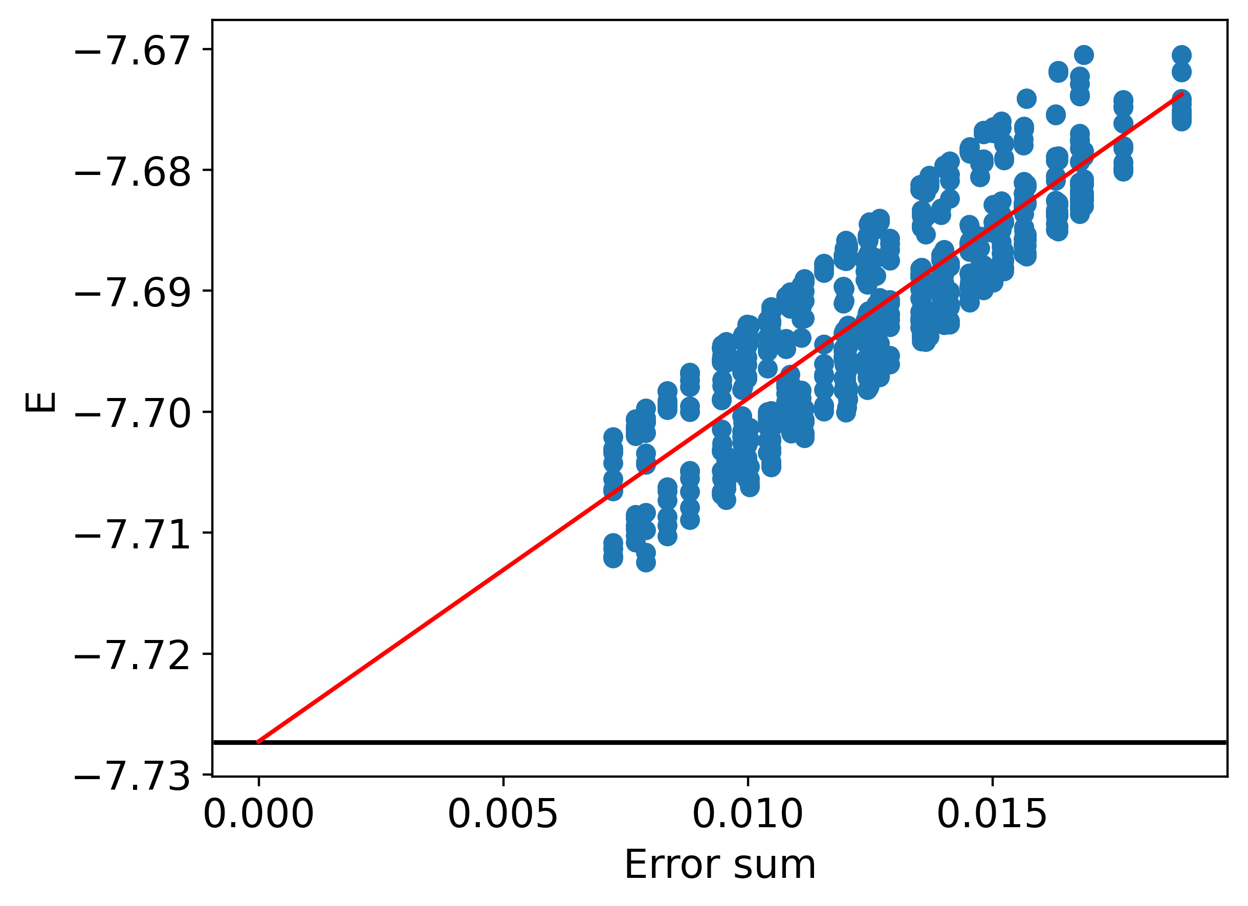
(a)

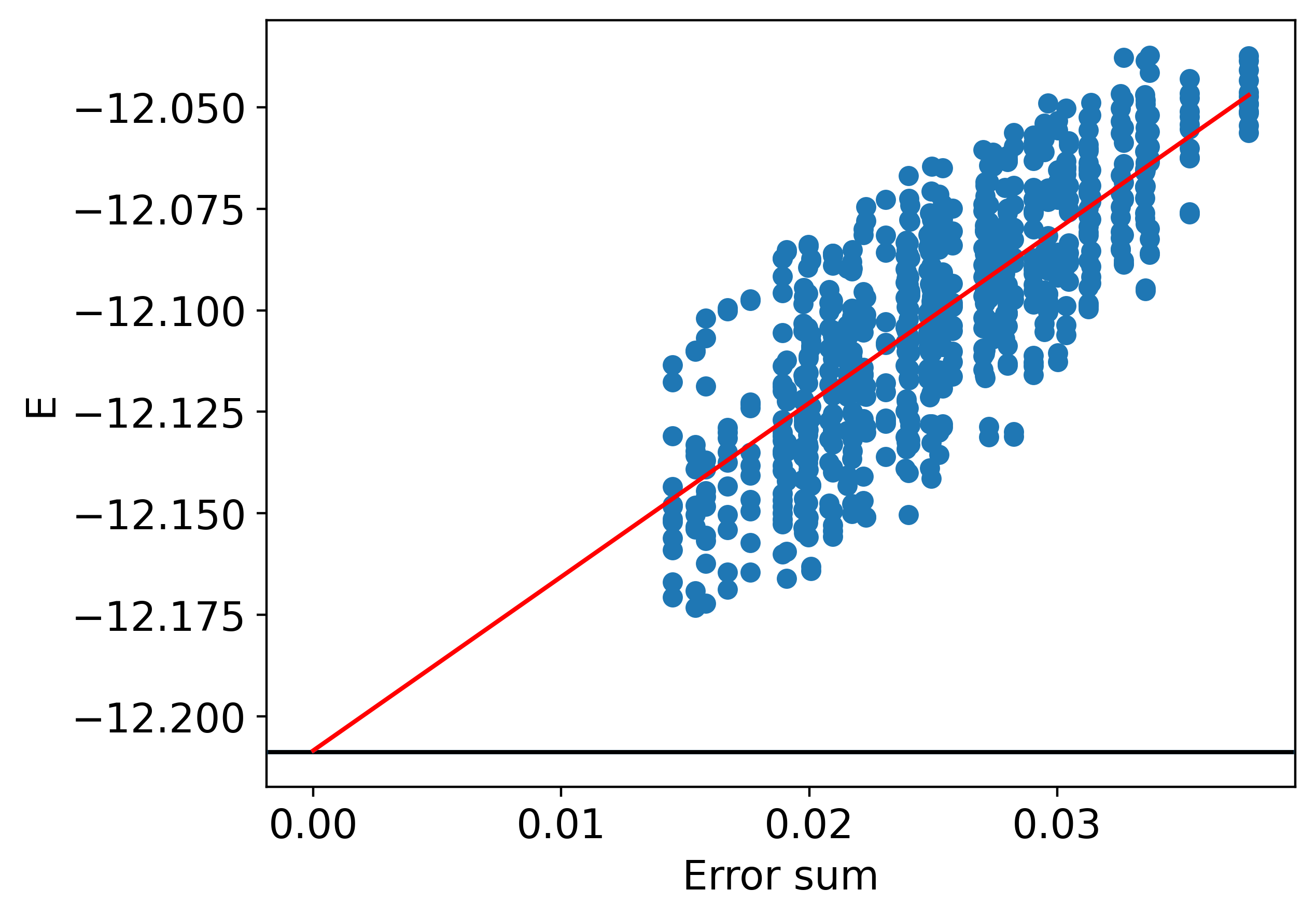
(b)

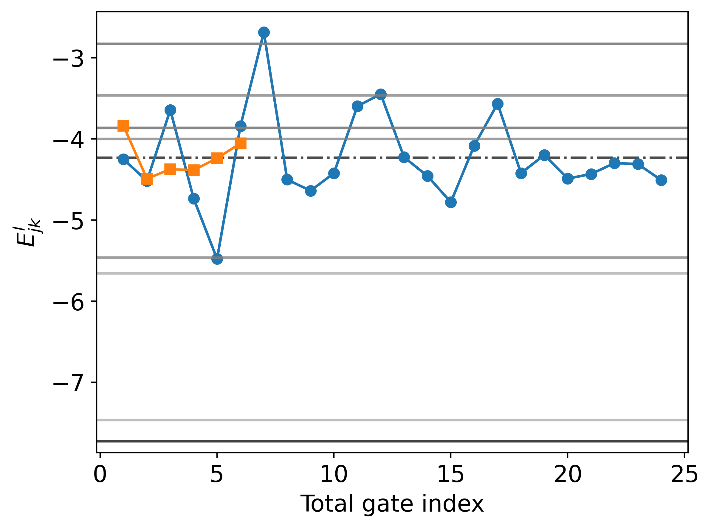
(c)

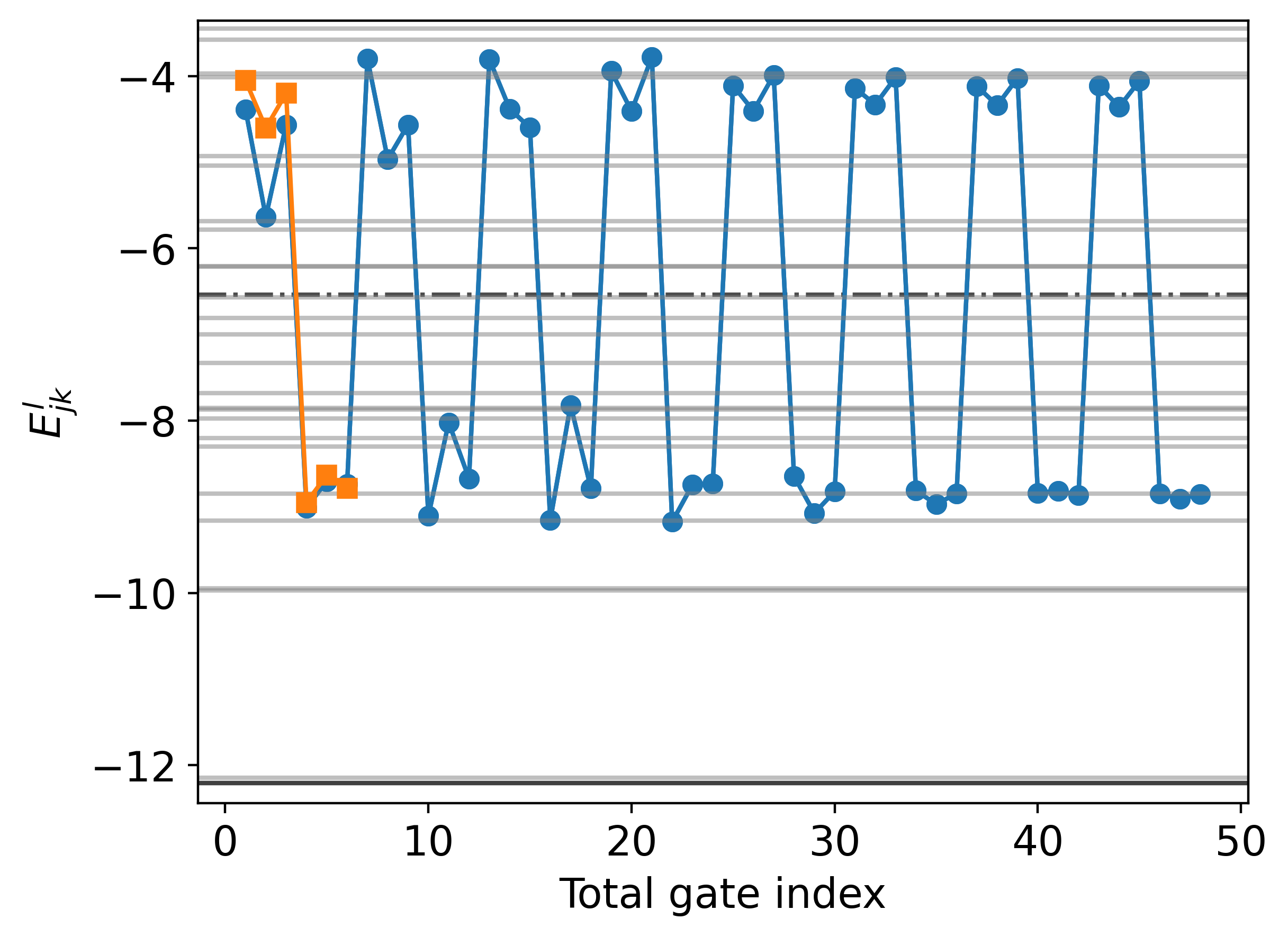
(d)

Figure 1: Zero-noise extrapolation (ZNE) using the proposed method. (a, b) ZNE for $n=6$ qubit problem Hamiltonians of type (a) and (b) respectively. In both plots the blue dots represent energy $E$ as per (8) for different permutations $\pi\in S_{n}$ and the red line is a linear fit taken over energies corresponding to all possible permutations. (c, d) The energies $E_{jk}^{l}$ (see (7)) for Hamiltonians of type (a) and (b) respectively (shown in circles). The squares show the perturbation energies averaged over the layers of the ansatz $\frac{1}{d}\sum_{l}E_{jk}^{l}$. The gray lines represent the eigenvalues of the Hamiltonian. The dash-dotted lines depict the average perturbation energy $A$. On all the panels black horizontal lines show the noiseless VQE energy.

(a)

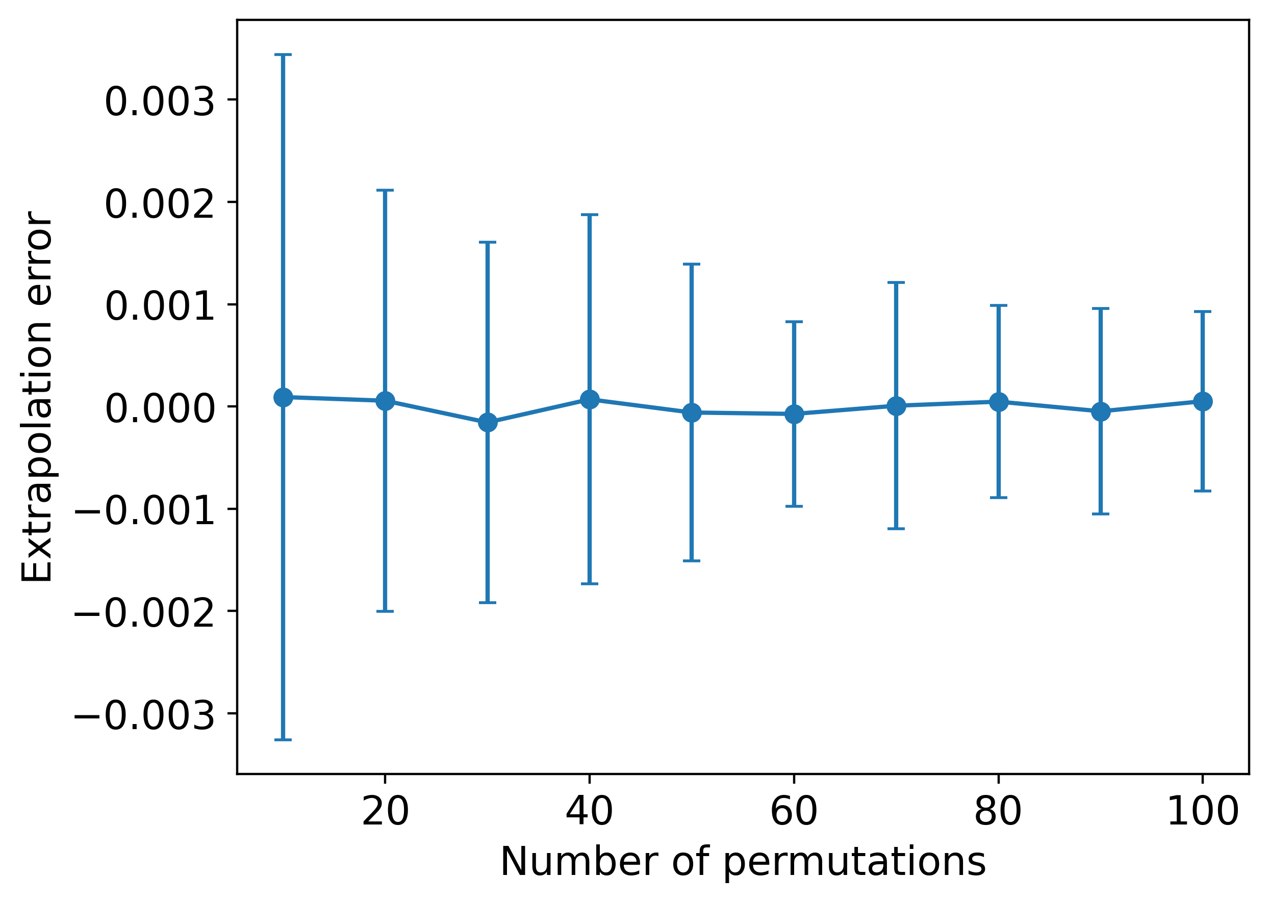
(b)

Figure 2: Zero-noise extrapolation (ZNE) with energies obtained from a finite number of randomly sampled permutations. The error bars show the standard deviation estimated from $50$ runs of the experiment. (a) Convergence of the ZNE error (difference between the energy estimated by ZNE and the ground state energy approximated by VQE under noiseless condition) for a Hardware efficient ansatz (HEA) with a ring topology. (b) The same for line topology. In both cases we have used a $n=6$ qubit Hamiltonian of type (a) as the problem Hamiltonian.

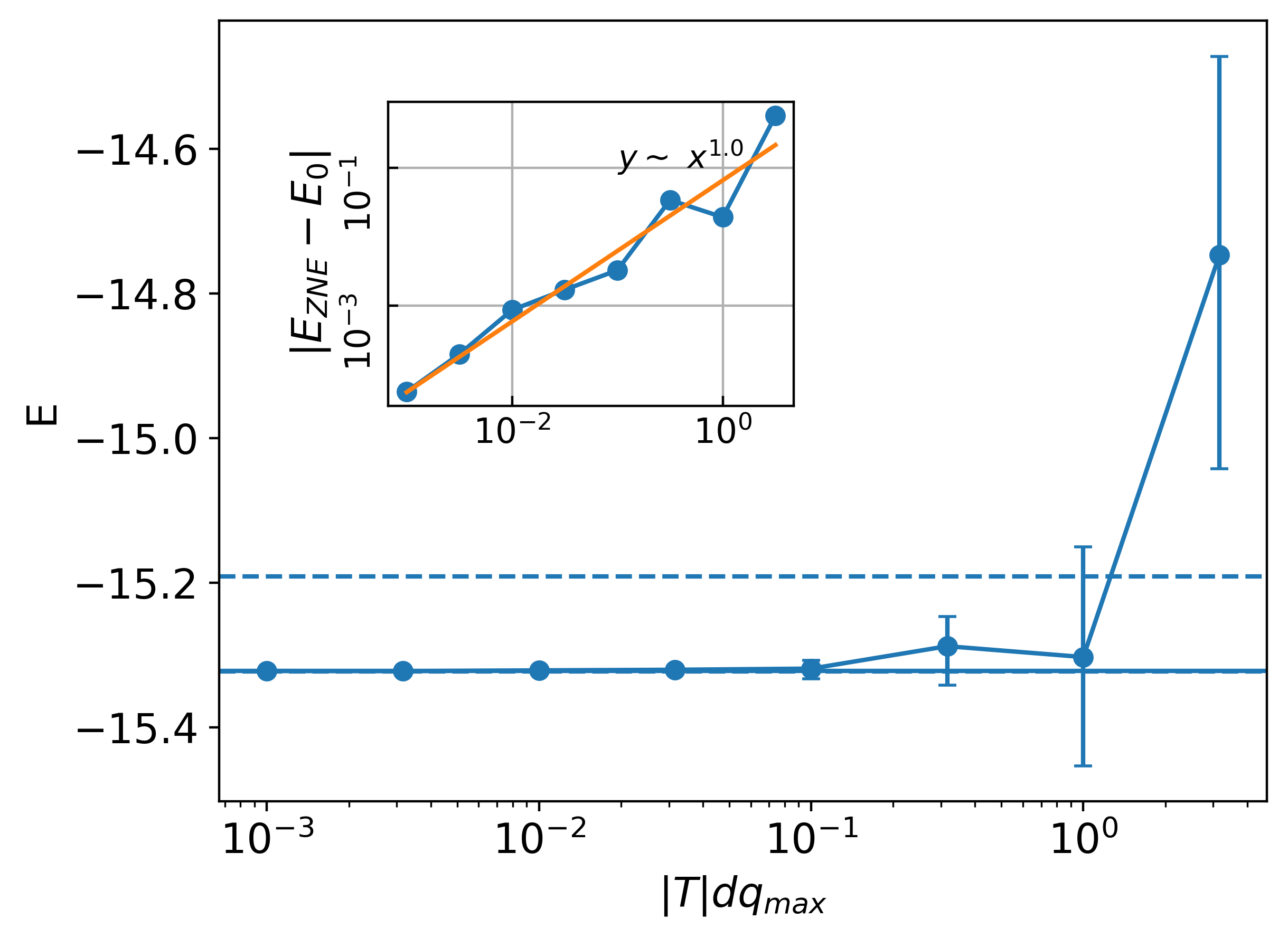
(a)

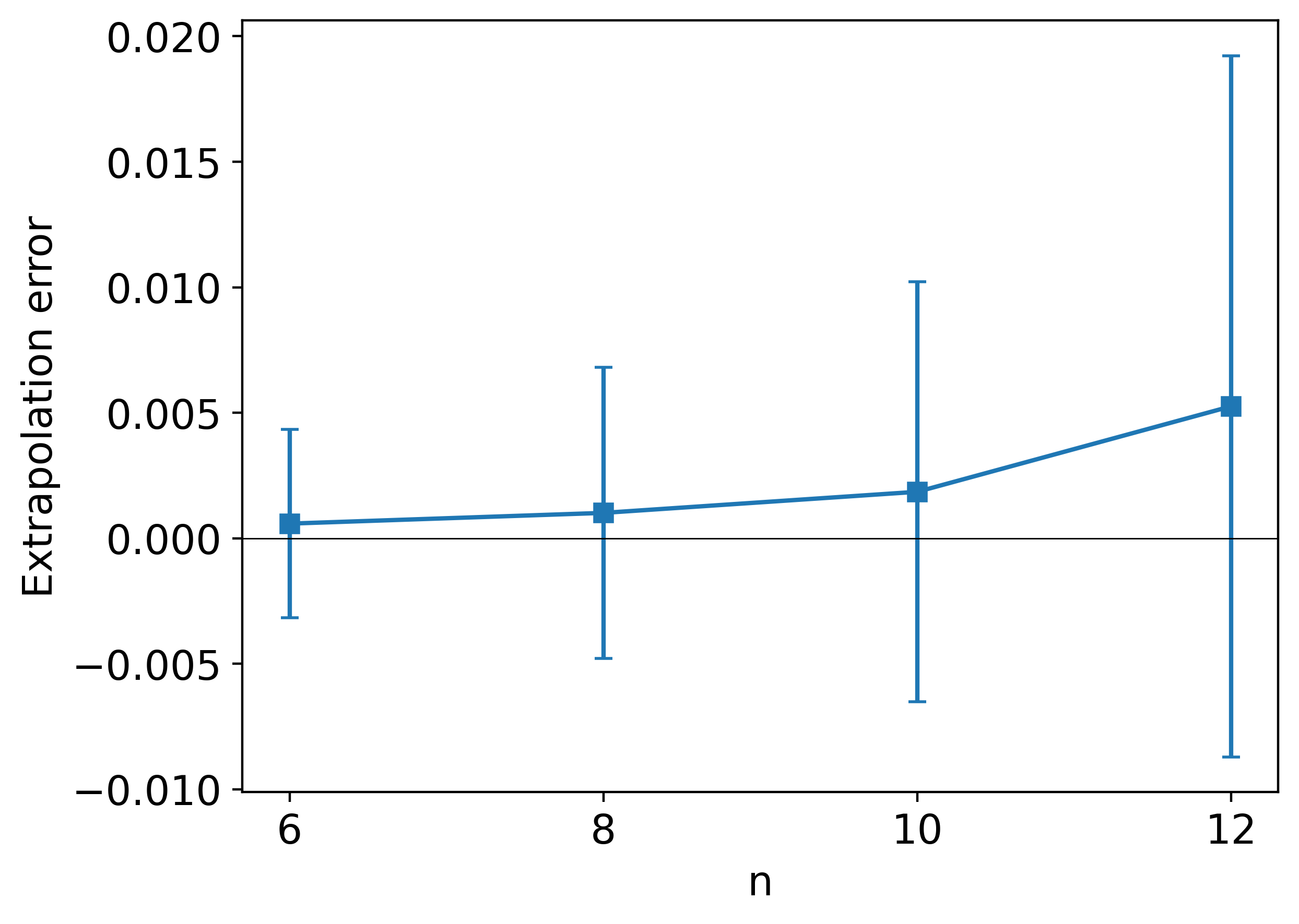
(b)

Figure 3: (a) ZNE estimated energy as a function of the magnitude of circuit errors for $n=12$ qubits. Solid horizontal line shows the noise-free VQE energy, dashed line shows the energy of the first excited state of the problem Hamiltonian. The error bars of the extrapolated energies are 95% confidence intervals obtained by bias-corrected and accelerated (BCa) boostrapping. The insets show the absolute value of the extrapolation error along with a linear fit in the double logarithmic scale. (b) Scaling of the extrapolation error for different $n$ when $q_{max}=10^{-3}$. The error bars show the standard deviation estimated from $50$ runs of the experiment.

III.2 ZNE with permutation fit

In this section we will lay down the recipe for ZNE assisted by inhomogeneous errors. Consider once again the variational circuit which we now want to implement on a physical device. Here one must make a distinction between the abstract qubits (ones in the circuit) and the physical qubits (ones in the device). We assume that it is possible to implement two-qubit gates on all pairs of physical qubits and we denote the corresponding error rates as $\bar{q}_{jk};j,k\in[1,n]$. If that is not the case, the number $\bar{q}_{jk}$ can simply denote the infidelity induced by all the extra swap gates required to implement the desired two-qubit gate.

In order to implement an $n$-qubit (abstract) circuit on an $n$-qubit (physical) device, one would first require to map the abstract qubits to their physical counterparts—what we call abstract-to-physical qubit mapping. Mathematically the mapping can be specified by a permutation $\pi\in S_{n}$ such that an abstract qubit indexed $j$ is mapped to the physical qubit indexed $\pi(j)$. Thus under the chosen qubit mapping the error rate associated with the gate $G^{l}_{jk}$, operating on the abstract qubit pair $(j,k)$ and hence the physical qubit pair $(\pi(j),\pi(k))$, will be denoted as $\bar{q}_{\pi(j)\pi(k)}\equiv\bar{q}_{\pi(jk)}$. For this choice of qubit mapping, the energy of the VQE ansatz state (7) transforms into the following:

$$E-E_{0}=d(A-E_{0})\sum_{(j,k)\in T}\bar{q}_{\pi(jk)}+\sum_{\begin{subarray}{c}(j,k)\in T\\ l\in[1,d]\end{subarray}}\bar{q}_{\pi(jk)}\epsilon^{l}_{jk}+O(q^{2}).$$ (8)

Evidently, for a generic ansatz circuit the sum $\sum\bar{q}_{\pi(jk)}$ will depend on the permutation $\pi$ and hence on the abstract-to-physical qubit mapping. Thus, by taking a number of permutations, we obtain the energies for different circuit error sums which can be approximated by a linear dependence of the form $E=a\sum\bar{q}_{\pi(jk)}+b$, where the slope $a$ approximates the term $d(A-E_{0})$, and the interception point $b$ approximates the noise-free energy $E_{0}$. Consequently, by making a linear fit through the noisy data, one could recover an approximation to the noiseless energy $E_{0}$. In general one cannot guarantee that the estimate constructed this way is exact. However, in Appendix B we show that this method of ZNE, when performed over all permutations $\pi\in S_{n}$, can recover the exact value of the noise-free energy for ansatz structures corresponding to regular graphs, in the limit of small errors $\bar{q}_{jk}$.

III.3 Numerical results

In this section we demonstrate ZNE using VQE with the transverse field Ising model as the problem Hamiltonian:

$$H=\sum_{j=1}^{n}J_{j}Z_{j}Z_{j+1}+\sum_{j=1}^{n}h_{j}X_{j},$$ (9)

where we set $Z_{1}=Z_{n+1}$. We consider two cases—(a) when $J_{j}=h_{j}=1$ and (b) when $J_{1}=6$, $J_{j}=1\leavevmode\nobreak\ \forall j\neq 1$ and $h_{j}=1$. The justification for the choice of parameters in the Hamiltonians of type (b) will become clear later in the text. We minimise (9) with respect to variational states prepared by a Hardware Efficient Ansatz (HEA) with ring topology. That is, in each layer we apply single-qubit gates to each qubit ($R_{Y}$, then $R_{X}$), then we apply two-qubit $R_{ZZ}$ gates to nearest neighboring qubits, as well as to the qubit pair $(n,1)$. The optimization is done in the Qiskit statevector simulator using the Limited memory Broyden–Fletcher–Goldfarb–Shanno (L-BFGS-B) algorithm. The starting point for the optimization is chosen by picking every parameter at random from the normal distribution with mean zero and $\sigma=10^{-3}$. The optimized circuit is then subjected to the noise and permutations of physical qubits. Each two-qubit gate is appended with a depolarizing noise channel with strength $\{\bar{q}_{jk}\}$ sampled from a uniform distribution on the interval $[0,0.001]$ with the condition $\bar{q}_{jk}=\bar{q}_{kj}$.

In Figs. 1(a) and 1(b) we demonstrate zero-noise extrapolation for Ising Hamiltonians of type (a) and (b) respectively with $n=6$. Each point in Fig. 1(a), 1(b) represents the energy $E$ obtained for a specific permutation $\pi\in S_{n}$. The depth of the ansatz circuit is chosen so that the VQE energy does not exceed the true ground state energy of the Hamiltonian by more than $10^{-2}$ times the spectral gap of the problem. In our case, the required depths are 4 and 8 for the Hamiltonians of type (a) and (b). The optimized VQE energies obtained at these optimal depths are $3\times 10^{-4}$ and $10^{-3}$ times the size of the spectral gap, respectively. Furthermore, we note that the optimal depths that we have obtained are associated to another peculiarity: as observed in larocca_theory_2023 , during Hamiltonian minimization, the error of the VQE energy against the exact ground state energy exhibits a sharp drop after a certain depth. This drop in our numerical experiments occurs exactly at the optimal depths.

For both Hamiltonians, performing ZNE over all permutations recovers the energy of the noiseless VQE approximation with a high accuracy. For the Hamiltonian of type (a), we recorded an extrapolation error of $6.7\times 10^{-5}$ (in units of $h_{j}$), which is more than 200 times smaller than the least energy obtained from the noisy circuits. For the Hamiltonian of type (b), the extrapolation error was $3.7\times 10^{-4}$ (in units of $h_{j}$), which is almost 100 times smaller than the least energy obtained from the noisy circuits.

Further we observe that the energies obtained for the Hamiltonians of type (a) better approximate a linear trend compared to the energies obtained for the Hamiltonians of type (b). To explain this behavior we recall that the deviation from the linear trend is governed by the non-uniformity of the energies $\epsilon_{jk}^{l}$, which is captured by the quantity $\text{max}\{\sum_{l}|\epsilon^{l}_{jk}|\}$ (see Appendix A). Figs. 1(c) and 1(d) illustrate that point: for the Hamiltonian of type (a), the energies $E_{jk}^{l}$ are more concentrated around the mean, and the linear trend with the CES is more apparent. At the same time, for the Hamiltonian of type (b) the distribution of the energies is wider, and consequently, the linear trend is less apparent.

The ZNE shown in Fig. 1 uses all possible permutations $\pi\in S_{n}$. However, taking all permutations is not feasible except for the smallest problems. In addition, in many quantum computer architectures, implementing an arbitrary permutation of a circuit is impossible without introducing additional swap gates. For example, while ion based quantum processors have all-to-all qubit connectivity, quantum processors based on superconducting qubits or trapped atoms do not. To address that, we investigated the performance of ZNE when only a small number of permutations is available. Fig. 2 shows the performance of ZNE as a function of the size of the permutation pool. Here we have considered a Hamiltonian of type (a) and minimized it using HEA with both ring and line topology, then introduced the depolarizing noise. While the extrapolation error increases for smaller size of the permutation pool, it is still centered around the noise-free energy, with the standard deviation being much smaller than any energy scale of the problem (spectral gap being $\sim 0.26$).

In the theoretical analysis, we demanded that $(\max\{q_{jk}\})|T|d\ll 1$ in order to discard the quadratic terms. However, this requirement can be restrictive for practical purposes. Thus, we investigate the real applicability range of the method. To do that, we took the setup of noise-free VQE for the Hamiltonian of type (a) and simulated the ZNE protocol with 50 random permutations across a wide range of noise amplitudes, for $n\in\{6,8,10,12\}$. The noise strengths are sampled from the uniform distribution on $[0,q_{max}]$, where we change $q_{max}$. The depth is again taken to be such that the error is below one percent of the spectral gap (respectively, 4, 7, 10, and 14 layers of the hardware-efficient ansatz), a figure which is again reached after a sharp drop in the error with respect to the depth.

The behavior of the ZNE approximation for $n=12$ is shown in Fig. 3(a); the other cases demonstrate qualitatively the same behavior. Up to $(\max\{q_{jk}\})|T|d\sim 1$, the ZNE error was smaller than the spectral gap of the problem. Moreover, even for larger values of $(\max\{q_{jk}\})|T|d$ the extrapolation was closer to the true ground state energy than any of the noisy energy values. In general, the absolute value of the extrapolation error appears to scale linearly with the amplitude of the noise (Fig. 3(a), inset).

The proposed method relies on the inhomogeneity of the error rates, essentially taking sums of error rates over particular subsets of qubit pairs. For larger system sizes and circuits, however, the sum of error rates converges towards the mean, leading to the concentration of circuit error sums. This might induce an instability in the ZNE estimated energy. To investigate this instability, we perform ZNE for system sizes $n\in\{6,8,10,12\}$ with $q_{max}=0.001$. For each $n$ we perform 50 experiments; in every experiment ZNE was performed for 50 random permutations. The resulting distributions of ZNE extrapolation error are shown in Fig. 3(b). We note that the standard deviation increases gradually with respect to $n$. One can offset this increase in the standard deviation by averaging the ZNE energy over at most polynomially (with respect to $n$) many experiments.

IV Conclusions

Existing studies on the behavior of VQE-estimated energy with respect to noise primarily focus on homogeneous error models fontana_evaluating_2021 ; dalton_variational_2022 ; kattemolle_effects_2022 ; rabinovich2022gate . While the linear trend in this case is well-established, this does not automatically translate to the case of inhomogeneous noise. Motivated by the fact that gate errors are inhomogeneously distributed across pairs of qubits in physical hardware, we propose a new method for zero-noise extrapolation. In particular, we showed that by changing the abstract-to-physical qubit mapping, it is possible to vary the level of noise in a quantum circuit in a controllable way. This enables us to execute ZNE in an experimentally amenable manner.

Applying this method to VQE, we found that the energy approximated by a noisy VQE circuit is approximately linear with respect to the circuit error sum. An analytic bound was derived to quantify the quality of the approximation. We found that this bound depends on the nature of the problem Hamiltonian and the error rates. We numerically demonstrated that using the proposed method for ZNE, one can approximate the energy estimated by noiseless VQE with high accuracy, reducing the noise-induced error by approximately two orders of magnitude. We have further showed that ZNE extrapolation error is smaller than all energy scales of the problem, even when extrapolating over less than $10\%$ of all possible permutations. Finally, we demonstrated that while increasing the system size does induce some instability in the ZNE protocol, it can be removed with at most polynomially many permutations.

Appendix A Relative deviation from linear trend in Eq. (7)

We begin our analysis with a simplified form of (7) for the sake of brevity:

$$y=\Delta x+\delta y,$$ (10)

where $y=(E-E_{0})$, $\Delta=(A-E_{0})$, $x=\sum_{(j,k)\in T}dq_{jk}$ and $\delta y=\sum_{(j,k)\in T}(\sum_{l\in[1,d]}\epsilon^{l}_{jk})q_{jk}=\sum_{(j,k)\in T}\tilde{\epsilon}_{jk}q_{jk}$. Taking into account that both $x$ and $\delta y$ are error rate dependent terms, one can consequently conclude that $\delta y$ represents a deviation from the linear dependence $y=\Delta x$. Nevertheless, one can upper bound the deviation $\delta y$ between the actual function $y$ as per (10) and the linear dependence $y=\Delta x$. To accomplish this we consider the relative deviation:

$$\frac{|\delta y|}{\Delta x}=\frac{|\sum_{(j,k)\in T}\tilde{\epsilon}_{jk}q_{jk}|}{d(A-E_{0})\sum_{(j,k)\in T}q_{jk}}$$ (11)

One can readily establish a bound on this quantity as:

$$\frac{|\delta y|}{\Delta x}\leq\frac{\text{max}\{|\tilde{\epsilon}_{jk}|\}_{(j,k)\in T}}{d(A-E_{0})}=B_{1}$$ (12)

This bound is not necessarily tight; however, one can improve it by taking into account the distribution of the error rates themselves:

$$\frac{|\delta y|}{\Delta x}\leq\frac{|T|\text{max}\{|\tilde{\epsilon}_{jk}|\}_{(j,k)\in T}\text{Diam}\{q_{jk}\}_{(j,k)\in T}}{d(A-E_{0})\sum_{(j,k)\in T}q_{jk}}=B_{2}.$$ (13)

Here $\text{Diam}\{A\}$ is the diameter of a set $A$. Combining (14) and (13) we arrive at the final result:

$$\frac{|\delta y|}{\Delta x}\leq\text{min}\{B_{1},B_{2}\}$$ (14)

Appendix B The zero-noise extrapolation over all permutations is exact

Consider the function:

$$y=\Delta x+\delta y.$$ (15)

We note that (15) maps to (8) when $y=(E-E_{0})$, $\Delta=(A-E_{0})$, $x=\sum_{(j,k)\in T}d\bar{q}_{\pi(jk)}$ and $\delta y=\sum_{(j,k)\in T}(\sum_{l\in[1,d]}\epsilon^{l}_{jk})\bar{q}_{\pi(jk)}=\sum_{(j,k)\in T}\tilde{\epsilon}_{jk}\bar{q}_{\pi(jk)}$. In our approach of zero-noise extrapolation we fit a linear approximation of the form $y=\alpha+\beta x$ to the function in (15). The constants $\alpha$ and $\beta$ are inferred by the least squares method where they have standard expressions in terms of sample statistics:

$$\alpha =\langle y\rangle-\beta\langle x\rangle$$ (16)

$$\beta =\frac{\operatorname{Cov}(x,y)}{\operatorname{Var}x}.$$ (17)

Here the angular brackets denote averaging over all samples (in our case, over all abstract-to-physical qubit mappings labelled by $\pi\in S_{n}$). Substituting (15) and (17) in (16), we obtain:

$$\alpha=-\langle x\rangle\frac{\operatorname{Cov}(x,\delta y)}{\operatorname{Var}x}.$$ (18)

Recall that for an exact zero-noise extrapolation we would get $\alpha=0$. In deriving (18) we have used the result $\langle\delta y\rangle=0$. This follows from two facts:

1. $\langle\bar{q}_{\pi(jk)}\rangle=\frac{1}{n!}\sum_{\pi\in S_{n}}\bar{q}_{\pi(jk)}=\bar{q}_{a}$, where $\bar{q}_{a}$ is the average error;

2. $\sum_{(j,k)\in T}\tilde{\epsilon}_{jk}=0$ by definition.

Now we consider the covariance $\operatorname{Cov}(x,\delta y)$ in more detail. Owing to the fact that $\langle\delta y\rangle=0$ we get

$$\operatorname{Cov}(x,\delta y)=\langle x\delta y\rangle=\frac{1}{n!}\sum_{\begin{subarray}{c}(j_{1},k_{1})\in T\\ (j_{2},k_{2})\in T\end{subarray}}\tilde{\epsilon}_{j_{1}k_{1}}\langle\bar{q}_{\pi(j_{1}k_{1})}\bar{q}_{\pi(j_{2}k_{2})}\rangle$$ (19)

We now group the summands in (19) such that (a) $j_{2}=j_{1},k_{2}=k_{1}$ (b) $j_{2}=j_{1},k_{2}\neq k_{1}$ or $j_{2}\neq j_{1},k_{2}=k_{1}$ and (c) $j_{2}\neq j_{1},k_{2}\neq k_{1}$. Denoting the average $\langle\bar{q}_{\pi(j_{1}k_{1})}\bar{q}_{\pi(j_{2}k_{2})}\rangle$ for the aforementioned cases to be $\kappa_{2},\kappa_{1}$ and $\kappa_{0}$ respectively, we arrive at the expression:

$$\operatorname{Cov}(x,\delta y)=\sum_{(jk)\in T}\tilde{\epsilon}_{jk}\left[n_{2}^{(jk)}\kappa_{2}+n_{1}^{(jk)}\kappa_{1}+n_{0}^{(jk)}\kappa_{0}\right].$$ (20)

Here $n_{2}^{(jk)}$ is the number of two-qubit gates acting on the qubit pair $(j,k)$, $n_{1}^{(jk)}$ is the number of two-qubit gates acting either on the qubit $j$ or $k$ and $n_{0}^{(jk)}$ is the number of gates that does not act either on $j$ or $k$. If these three values are independent on $(j,k)$, the covariance $\operatorname{Cov}(x,\delta y)$ vanishes owing to the fact that $\sum_{(j,k)\in T}\tilde{\epsilon}_{jk}=0$ implying that $\alpha=0$, which is what we expected for an exact zero-noise extrapolation.

We note here that $n_{2}^{(jk)}$, $n_{1}^{(jk)}$, $n_{0}^{(jk)}$ are independent of $(j,k)$ only for specific ansatz circuits. To characterise the structure of such ansatze completely we depict the ansatz circuit as a multigraph with vertices corresponding to qubits and edges corresponding to two-qubit gates. Indeed $n_{2}^{(jk)}$ is the count of gates acting on $(j,k)$, $n_{1}^{(jk)}=\deg(j)+\deg(k)-n_{2}^{(jk)}$, and $n_{0}^{(jk)}=|T|d-n_{1}^{(jk)}-n_{2}^{(jk)}$. Thus, these values only depend on degrees of vertices and multiplicities of edges. This implies that the gate-independence condition can be satisfied by taking a regular graph (e.g. a cycle) as the structure of the ansatz.

References

- (1) Matthew P Harrigan, Kevin J Sung, Matthew Neeley, Kevin J Satzinger, Frank Arute, Kunal Arya, Juan Atalaya, Joseph C Bardin, Rami Barends, Sergio Boixo, et al. Quantum approximate optimization of non-planar graph problems on a planar superconducting processor. Nature Physics, 17(3):332–336, 2021.
- (2) Guido Pagano, Aniruddha Bapat, Patrick Becker, Katherine S. Collins, Arinjoy De, Paul W. Hess, Harvey B. Kaplan, Antonis Kyprianidis, Wen Lin Tan, Christopher Baldwin, Lucas T. Brady, Abhinav Deshpande, Fangli Liu, Stephen Jordan, Alexey V. Gorshkov, and Christopher Monroe. Quantum approximate optimization of the long-range Ising model with a trapped-ion quantum simulator. Proceedings of the National Academy of Sciences, 117(41):25396–25401, 2020.
- (3) Gian Giacomo Guerreschi and Anne Y Matsuura. QAOA for Max-Cut requires hundreds of qubits for quantum speed-up. Scientific Reports, 9(1):1–7, 2019.
- (4) Anastasiia Butko, George Michelogiannakis, Samuel Williams, Costin Iancu, David Donofrio, John Shalf, Jonathan Carter, and Irfan Siddiqi. Understanding quantum control processor capabilities and limitations through circuit characterization. In 2020 International Conference on Rebooting Computing (ICRC), pages 66–75. IEEE, 2020.
- (5) Murphy Yuezhen Niu, Sirui Lu, and Isaac L. Chuang. Optimizing qaoa: Success probability and runtime dependence on circuit depth. arXiv:1905.12134.
- (6) Edward Farhi, Jeffrey Goldstone, and Sam Gutmann. A quantum approximate optimization algorithm. arXiv:1411.4028.
- (7) Seth Lloyd. Quantum approximate optimization is computationally universal. arXiv:1812.11075.
- (8) Mauro ES Morales, JD Biamonte, and Zoltán Zimborás. On the universality of the quantum approximate optimization algorithm. Quantum Information Processing, 19(9):1–26, 2020.
- (9) Edward Farhi and Aram W Harrow. Quantum supremacy through the quantum approximate optimization algorithm. arXiv:1602.07674.
- (10) V. Akshay, H. Philathong, M. E.S. Morales, and J. D. Biamonte. Reachability Deficits in Quantum Approximate Optimization. Physical Review Letters, 124(9):090504, Mar 2020.
- (11) Edward Farhi, Jeffrey Goldstone, Sam Gutmann, and Leo Zhou. The Quantum Approximate Optimization Algorithm and the Sherrington-Kirkpatrick Model at Infinite Size. Quantum, 6:759, July 2022.
- (12) Matteo M. Wauters, Glen Bigan Mbeng, and Giuseppe E. Santoro. Polynomial scaling of QAOA for ground-state preparation of the fully-connected p-spin ferromagnet. arXiv:2003.07419.
- (13) V. Akshay, D. Rabinovich, E. Campos, and J. Biamonte. Parameter concentrations in quantum approximate optimization. Phys. Rev. A, 104:L010401, Jul 2021.
- (14) E Campos, D Rabinovich, V Akshay, and J Biamonte. Training saturation in layerwise quantum approximate optimisation. (Letter) Physical Review A, 104:L030401, 2021.
- (15) Daniil Rabinovich, Richik Sengupta, Ernesto Campos, Vishwanathan Akshay, and Jacob Biamonte. Progress towards analytically optimal angles in quantum approximate optimisation. Mathematics, 10(15):2601, 2022.
- (16) V. Akshay, H. Philathong, E. Campos, D. Rabinovich, I. Zacharov, Xiao-Ming Zhang, and J. D. Biamonte. Circuit depth scaling for quantum approximate optimization. Phys. Rev. A, 106:042438, Oct 2022.
- (17) Daniil Rabinovich, Soumik Adhikary, Ernesto Campos, Vishwanathan Akshay, Evgeny Anikin, Richik Sengupta, Olga Lakhmanskaya, Kirill Lakhmanskiy, and Jacob Biamonte. Ion-native variational ansatz for quantum approximate optimization. Phys. Rev. A, 106:032418, Sep 2022.
- (18) Alberto Peruzzo, Jarrod McClean, Peter Shadbolt, Man-Hong Yung, Xiao-Qi Zhou, Peter J. Love, Alán Aspuru-Guzik, and Jeremy L. O’Brien. A variational eigenvalue solver on a photonic quantum processor. Nature Communications, 5(1):4213, December 2014.
- (19) Yudong Cao, Jonathan Romero, Jonathan P Olson, Matthias Degroote, Peter D Johnson, Mária Kieferová, Ian D Kivlichan, Tim Menke, Borja Peropadre, Nicolas PD Sawaya, et al. Quantum chemistry in the age of quantum computing. Chemical Reviews, 119(19):10856–10915, 2019.
- (20) Sam McArdle, Suguru Endo, Alán Aspuru-Guzik, Simon C Benjamin, and Xiao Yuan. Quantum computational chemistry. Reviews of Modern Physics, 92(1):015003, 2020.
- (21) Dave Wecker, Matthew B Hastings, and Matthias Troyer. Progress towards practical quantum variational algorithms. Physical Review A, 92(4):042303, 2015.
- (22) Bela Bauer, Dave Wecker, Andrew J Millis, Matthew B Hastings, and Matthias Troyer. Hybrid quantum-classical approach to correlated materials. Physical Review X, 6(3):031045, 2016.
- (23) Jacob Biamonte, Peter Wittek, Nicola Pancotti, Patrick Rebentrost, Nathan Wiebe, and Seth Lloyd. Quantum machine learning. Nature, 549(7671):195–202, 2017.
- (24) Maria Schuld and Nathan Killoran. Quantum machine learning in feature hilbert spaces. Physical Review Letters, 122(4):040504, 2019.
- (25) Soumik Adhikary, Siddharth Dangwal, and Debanjan Bhowmik. Supervised learning with a quantum classifier using multi-level systems. Quantum Information Processing, 19:1–12, 2020.
- (26) Soumik Adhikary. Entanglement assisted training algorithm for supervised quantum classifiers. Quantum Information Processing, 20(8):254, 2021.
- (27) Vojtěch Havlíček, Antonio D Córcoles, Kristan Temme, Aram W Harrow, Abhinav Kandala, Jerry M Chow, and Jay M Gambetta. Supervised learning with quantum-enhanced feature spaces. Nature, 567(7747):209–212, 2019.
- (28) Enrico Fontana, Nathan Fitzpatrick, David Muñoz Ramo, Ross Duncan, and Ivan Rungger. Evaluating the noise resilience of variational quantum algorithms. Physical Review A, 104(2):022403, August 2021.
- (29) Samson Wang, Enrico Fontana, M. Cerezo, Kunal Sharma, Akira Sone, Lukasz Cincio, and Patrick J. Coles. Noise-induced barren plateaus in variational quantum algorithms. Nature Communications, 12(1):6961, November 2021.
- (30) Zhenyu Cai, Ryan Babbush, Simon C Benjamin, Suguru Endo, William J Huggins, Ying Li, Jarrod R McClean, and Thomas E O’Brien. Quantum error mitigation. arXiv:2210.00921.
- (31) Sergey Bravyi, Sarah Sheldon, Abhinav Kandala, David C. Mckay, and Jay M. Gambetta. Mitigating measurement errors in multiqubit experiments. Physical Review A, 103(4):042605, April 2021.
- (32) Piotr Czarnik, Andrew Arrasmith, Patrick J. Coles, and Lukasz Cincio. Error mitigation with Clifford quantum-circuit data. Quantum, 5:592, November 2021.
- (33) Suguru Endo, Simon C. Benjamin, and Ying Li. Practical Quantum Error Mitigation for Near-Future Applications. Physical Review X, 8(3):031027, July 2018.
- (34) Angus Lowe, Max Hunter Gordon, Piotr Czarnik, Andrew Arrasmith, Patrick J. Coles, and Lukasz Cincio. Unified approach to data-driven quantum error mitigation. Physical Review Research, 3(3):033098, July 2021.
- (35) Filip B. Maciejewski, Zoltán Zimborás, and Michał Oszmaniec. Mitigation of readout noise in near-term quantum devices by classical post-processing based on detector tomography. Quantum, 4:257, April 2020.
- (36) Bibek Pokharel, Namit Anand, Benjamin Fortman, and Daniel A. Lidar. Demonstration of Fidelity Improvement Using Dynamical Decoupling with Superconducting Qubits. Physical Review Letters, 121(22):220502, November 2018.
- (37) Kristan Temme, Sergey Bravyi, and Jay M. Gambetta. Error Mitigation for Short-Depth Quantum Circuits. Physical Review Letters, 119(18):180509, November 2017.
- (38) Lorenza Viola and Seth Lloyd. Dynamical suppression of decoherence in two-state quantum systems. Physical Review A, 58(4):2733–2744, October 1998.
- (39) Shuaining Zhang, Yao Lu, Kuan Zhang, Wentao Chen, Ying Li, Jing-Ning Zhang, and Kihwan Kim. Error-mitigated quantum gates exceeding physical fidelities in a trapped-ion system. Nature Communications, 11(1):587, January 2020.
- (40) Kristan Temme, Sergey Bravyi, and Jay M Gambetta. Error mitigation for short-depth quantum circuits. Physical Review Letters, 119(18):180509, 2017.
- (41) Ying Li and Simon C Benjamin. Efficient variational quantum simulator incorporating active error minimization. Physical Review X, 7(2):021050, 2017.
- (42) Abhinav Kandala, Kristan Temme, Antonio D. Córcoles, Antonio Mezzacapo, Jerry M. Chow, and Jay M. Gambetta. Error mitigation extends the computational reach of a noisy quantum processor. Nature, 567(7749):491–495, March 2019.
- (43) I. Pogorelov, T. Feldker, Ch. D. Marciniak, L. Postler, G. Jacob, O. Krieglsteiner, V. Podlesnic, M. Meth, V. Negnevitsky, M. Stadler, B. Höfer, C. Wächter, K. Lakhmanskiy, R. Blatt, P. Schindler, and T. Monz. Compact ion-trap quantum computing demonstrator. PRX Quantum, 2:020343, Jun 2021.
- (44) K. Wright, K. M. Beck, S. Debnath, J. M. Amini, Y. Nam, N. Grzesiak, J.-S. Chen, N. C. Pisenti, M. Chmielewski, C. Collins, K. M. Hudek, J. Mizrahi, J. D. Wong-Campos, S. Allen, J. Apisdorf, P. Solomon, M. Williams, A. M. Ducore, A. Blinov, S. M. Kreikemeier, V. Chaplin, M. Keesan, C. Monroe, and J. Kim. Benchmarking an 11-qubit quantum computer. Nature Communications, 10(1):5464, 2019.
- (45) Jacob Biamonte. Universal variational quantum computation. Physical Review A, 103(3):L030401, March 2021.
- (46) Harper R. Grimsley, Sophia E. Economou, Edwin Barnes, and Nicholas J. Mayhall. An adaptive variational algorithm for exact molecular simulations on a quantum computer. Nature Communications, 10(1):3007, December 2019.
- (47) Ho Lun Tang, V.O. Shkolnikov, George S. Barron, Harper R. Grimsley, Nicholas J. Mayhall, Edwin Barnes, and Sophia E. Economou. Qubit-ADAPT-VQE: An Adaptive Algorithm for Constructing Hardware-Efficient Ansätze on a Quantum Processor. PRX Quantum, 2(2):020310, April 2021.
- (48) Sukin Sim, Jonathan Romero, Jérôme F Gonthier, and Alexander A Kunitsa. Adaptive pruning-based optimization of parameterized quantum circuits. Quantum Science and Technology, 6(2):025019, April 2021.
- (49) M. Bilkis, M. Cerezo, Guillaume Verdon, Patrick J. Coles, and Lukasz Cincio. A semi-agnostic ansatz with variable structure for quantum machine learning. arXiv:2103.06712.
- (50) Mariia D. Sapova and Aleksey K. Fedorov. Variational quantum eigensolver techniques for simulating carbon monoxide oxidation. Communications Physics, 5(1):199, August 2022.
- (51) Kosuke Mitarai, Makoto Negoro, Masahiro Kitagawa, and Keisuke Fujii. Quantum Circuit Learning. Physical Review A, 98(3):032309, September 2018.
- (52) Maria Schuld, Ville Bergholm, Christian Gogolin, Josh Izaac, and Nathan Killoran. Evaluating analytic gradients on quantum hardware. Physical Review A, 99(3):032331, March 2019.
- (53) Oleksandr Kyriienko and Vincent E. Elfving. Generalized quantum circuit differentiation rules. Physical Review A, 104(5):052417, November 2021.
- (54) Vladyslav Verteletskyi, Tzu-Ching Yen, and Artur F. Izmaylov. Measurement optimization in the variational quantum eigensolver using a minimum clique cover. The Journal of Chemical Physics, 152(12):124114, March 2020.
- (55) Panagiotis Kl Barkoutsos, Jerome F. Gonthier, Igor Sokolov, Nikolaj Moll, Gian Salis, Andreas Fuhrer, Marc Ganzhorn, Daniel J. Egger, Matthias Troyer, Antonio Mezzacapo, Stefan Filipp, and Ivano Tavernelli. Quantum algorithms for electronic structure calculations: Particle/hole Hamiltonian and optimized wavefunction expansions. Physical Review A, 98(2), August 2018.
- (56) Jules Tilly, Hongxiang Chen, Shuxiang Cao, Dario Picozzi, Kanav Setia, Ying Li, Edward Grant, Leonard Wossnig, Ivan Rungger, George H. Booth, and Jonathan Tennyson. The Variational Quantum Eigensolver: A review of methods and best practices. Physics Reports, 986:1–128, November 2022.
- (57) Yudong Cao, Jonathan Romero, Jonathan P. Olson, Matthias Degroote, Peter D. Johnson, Mária Kieferová, Ian D. Kivlichan, Tim Menke, Borja Peropadre, Nicolas P. D. Sawaya, Sukin Sim, Libor Veis, and Alán Aspuru-Guzik. Quantum Chemistry in the Age of Quantum Computing. Chemical Reviews, 119(19):10856–10915, October 2019.
- (58) V. E. Elfving, B. W. Broer, M. Webber, J. Gavartin, M. D. Halls, K. P. Lorton, and A. Bochevarov. How will quantum computers provide an industrially relevant computational advantage in quantum chemistry? arXiv:2009.12472.
- (59) Nitzan Akerman, Nir Navon, Shlomi Kotler, Yinnon Glickman, and Roee Ozeri. Universal gate-set for trapped-ion qubits using a narrow linewidth diode laser. New Journal of Physics, 17(11):113060, nov 2015.
- (60) C. J. Ballance, T. P. Harty, N. M. Linke, M. A. Sepiol, and D. M. Lucas. High-fidelity quantum logic gates using trapped-ion hyperfine qubits. Phys. Rev. Lett., 117:060504, Aug 2016.
- (61) A. Bermudez, X. Xu, R. Nigmatullin, J. O’Gorman, V. Negnevitsky, P. Schindler, T. Monz, U. G. Poschinger, C. Hempel, J. Home, F. Schmidt-Kaler, M. Biercuk, R. Blatt, S. Benjamin, and M. Müller. Assessing the progress of trapped-ion processors towards fault-tolerant quantum computation. Phys. Rev. X, 7:041061, Dec 2017.
- (62) Harry Levine, Alexander Keesling, Ahmed Omran, Hannes Bernien, Sylvain Schwartz, Alexander S. Zibrov, Manuel Endres, Markus Greiner, Vladan Vuletić, and Mikhail D. Lukin. High-fidelity control and entanglement of rydberg-atom qubits. Phys. Rev. Lett., 121:123603, Sep 2018.
- (63) Colin D. Bruzewicz, John Chiaverini, Robert McConnell, and Jeremy M. Sage. Trapped-ion quantum computing: Progress and challenges. Applied Physics Reviews, 6(2):021314, June 2019.
- (64) Martín Larocca, Nathan Ju, Diego García-Martín, Patrick J. Coles, and Marco Cerezo. Theory of overparametrization in quantum neural networks. Nature Computational Science, 3(6):542–551, June 2023.
- (65) Kieran Dalton, Christopher K. Long, Yordan S. Yordanov, Charles G. Smith, Crispin H.W. Barnes, Normann Mertig, and David R.M. Arvidsson-Shukur. Variational quantum chemistry requires gate-error probabilities below the fault-tolerance threshold. arXiv:2211.04505.
- (66) Joris Kattemölle and Guido Burkard. Effects of correlated errors on the Quantum Approximate Optimization Algorithm. arXiv:2207.10622.
- (67) Daniil Rabinovich, Ernesto Campos, Soumik Adhikary, Ekaterina Pankovets, Dmitry Vinichenko, and Jacob Biamonte. On the gate-error robustness of variational quantum algorithms. arXiv:2301.00048.