The Interplay of Machine Learning–based
Resonant Anomaly Detection Methods

Abstract

Machine learning–based anomaly detection (AD) methods are promising tools for extending the coverage of searches for physics beyond the Standard Model (BSM). One class of AD methods that has received significant attention is resonant anomaly detection, where the BSM is assumed to be localized in at least one known variable. While there have been many methods proposed to identify such a BSM signal that make use of simulated or detected data in different ways, there has not yet been a study of the methods’ complementarity. To this end, we address two questions. First, in the absence of any signal, do different methods pick the same events as signal-like? If not, then we can significantly reduce the false-positive rate by comparing different methods on the same dataset. Second, if there is a signal, are different methods fully correlated? Even if their maximum performance is the same, since we do not know how much signal is present, it may be beneficial to combine approaches. Using the Large Hadron Collider (LHC) Olympics dataset, we provide quantitative answers to these questions. We find that there are significant gains possible by combining multiple methods, which will strengthen the search program at the LHC and beyond.

1 Introduction

Since the observation of the Higgs Boson in 2012 at the Large Hadron Collider (LHC) Aad:2012tfa ; Chatrchyan:2012ufa , no new fundamental particle has been observed. This is not for lack of effort: theoretical models involving supersymmetric particles, dark matter candidates, or heavy matter generations abound, informing past, current, and planned analyses at the LHC atlasexoticstwiki ; atlassusytwiki ; atlashdbspublictwiki ; cmsexoticstwiki ; cmssusytwiki ; cmsb2gtwiki ; lhcbtwiki . Given that such past searches for specific alternatives to the Standard Model (SM) have been unsuccessful, there has been a push to run broader, model-agnostic searches for new physics in parallel. In particular, machine learning (ML) has enabled many new search strategies Karagiorgi:2021ngt ; Kasieczka:2021xcg ; Aarrestad:2021oeb .

One of the most popular and well-motivated search strategies for evidence of physics beyond the Standard Model is resonant anomaly detection. In such investigations, the new physics signal is expected to take the form of a new particle, i.e. a resonance with respect to a mass-like event variable. The search strategy then involves looking for a localized excess of these new physics events with respect to the SM background.

There now exist many ML methods for resonant anomaly detection (AD) with comparable sensitivities Collins:2018epr ; Collins:2019jip ; Andreassen:2020nkr ; Nachman:2020lpy ; Benkendorfer:2020gek ; Stein:2020rou ; Amram_2021 ; Hallin:2021wme ; Kamenik:2022qxs ; Hallin:2022eoq ; Chen:2022suv ; Golling:2022nkl ; sengupta2023curtains , some of which have also been applied to data ATLAS:2020iwa ; Shih:2021kbt ; Shih:2023jfv ; Pettee:2023zra . These methods have largely been developed independently of each other, with different strengths and weaknesses. However, there has not yet been a thorough study of the complementarity of these techniques. In particular, we want to ask the questions: can we improve signal sensitivity by combining these methods? Can we improve robustness in the background-only case by combining them? Do these different methods classify the same things as “signal-like” for background and signal-like events?

In this paper, we evaluate a selection of these resonant AD methods on equal footing, using an identical methodological setup for each. In Sec. 2, we provide a more detailed background of the resonant AD procedure and introduce the four detection methods that we will consider in this paper. In Sec. 3, we consider how similar the detection methods are to each other, gauging whether different methods pick up distinct components of the phase space of resonant anomalies. In Sec. 4, we combine the four sample generation methods with the goal of increasing sensitivity for a resonant AD task. We conclude in Sec. 5, suggesting avenues for further exploration.

2 Methodology

2.1 Overview of resonant anomaly detection

The goal of resonant AD (illustrated schematically in Fig. 1) is to find an excess of beyond-the-Standard Model (BSM) events that are localized in some event variable $m$ (usually, a mass-like feature). The BSM signal thus corresponds to a new particle with a nonzero $m$, expected to be reconstructed within a signal region, SR, defined as an interval in $m$. In particular, the search makes use of a set of other (i.e. non-$m$) features in order to elevate the sensitivity above that of a standard bump hunt. Importantly, the excess events must be observed with respect to a SM background, but this background is nontrivial to construct: using out-of-the-box simulated data is not ideal given the numerous necessary approximations made for the hard-process, showering, and detector simulation steps; using actual data from outside of the signal region (or in sideband regions, SB) requires the analysis to only use event features that are statistically independent from the mass variable Collins:2018epr ; Collins:2019jip ; Benkendorfer:2020gek .

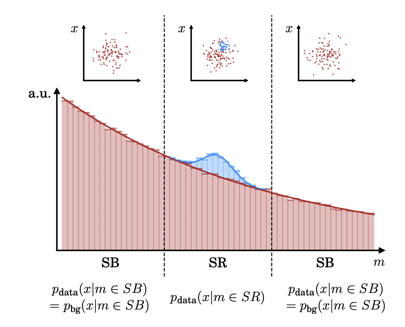
Figure 1: A schematic of the resonant anomaly detection motivation. The goal is to observe an excess of signal (blue) events above a background (red) process. The signal is localized in $m$ to a signal region (SR), and a model for background can be derived from data in the sidebands (SB) regions. Typically, the signal-background discrimination task makes use of features other than $m$. Figure is taken from Hallin:2021wme .

An alternative strategy is to construct a set of synthetic SM samples, or events that are representative of the SM background process in the same mass space as the BSM events. A binary classifier trained to discriminate the synthetic samples from detected data is then the optimal classifier for discriminating SM background from the new physics (see Ref. Metodiev:2017vrx ), so long as the synthetic samples are indeed a faithful representation of actual SM (i.e. not containing any events derived from a resonant anomaly) events in the probed mass range.

In recent years, there has been much work done on developing procedures to construct such synthetic SM samples. While there now exist many varied methods for sample construction, the vast majority of them can be characterized based on two properties of their construction. First, generation methods can be data-exclusive or simulation-assisted: data-exclusive methods generate synthetic samples by making use of collider data from the SB mass regions, where the data are far enough from any BSM signal to be treated as representative of SM background; simulation-assisted methods will also use an auxiliary dataset of simulated background-only collisions. Second, generation methods exploit machine learning techniques through either likelihood(-ratio) learning or feature morphing: methods can either learn the likelihood(-ratio) of a SM-only dataset (this can be either from the auxiliary simulated dataset or the SB data) and interpolate this likelihood into the SR; alternatively, methods can morph features from said background-only regions into the SR.

In this paper, we will consider the four methods shown in Table 1, which span this “character space” of methods for resonant AD.

	Simulation-assisted	Data-exclusive
Likelihood learning	Salad Andreassen:2020nkr	(La)Cathode Hallin:2021wme ; Hallin:2022eoq
Feature morphing	Feta Golling:2022nkl	Curtains sengupta2023curtains

Table 1: Many methods for constructing Standard Model background templates for resonant anomaly detection can be classified on two axes: on the horizontal, usage of an auxiliary dataset (simulation); on the vertical, how non-signal region Standard Model background processes are morphed into signal region Standard Model template samples.

We provide a brief summary of the four methods considered here.

• SALAD: Simulation Assisted Likelihood-free Anomaly Detection Andreassen:2020nkr trains a binary classifier to discriminate simulated SM events from detected SM events in the SB (background-only) region, then uses the classifier to reweight simulated SM events in the SR. These reweighted events comprise the synthetic SM samples.

• CATHODE: Classifying Anomalies THrough Outer Density Estimation Hallin:2021wme trains a normalizing flow–based probability density estimator to model detected data in SB, then interpolates the distribution into the SR. A set of events drawn from the interpolated distribution comprises the synthetic SM samples.

• CURTAINs: Constructing Unobserved Regions by Transforming Adjacent INtervals sengupta2023curtains trains a normalizing flow–based transport function to morph detected data between low- and high-mass SB, then applies the flow to map from SB into the SR. These morphed samples comprise the synthetic SM samples.

• FETA: Flow-Enhanced Transportation for Anomaly detection Golling:2022nkl trains a normalizing flow–based transport function to morph SM simulation in SB to detected data in background-dominated SB, then applies the model to SM simulation in the SR. These morphed samples comprise the synthetic SM samples.

Our goal is then to explore how the synthetic SM samples generated by each of these methods perform in resonant AD tasks, focusing on their relative performances in addition to their absolute performances. In fact, all four methods are comparable at picking up on signal contaminations of $\sim 0.93\%$ and above: in Fig. 2, we plot the significance improvement characteristic (SIC) as a function of the signal efficiency. Broadly speaking, the SIC corresponds to the multiplicative factor by which a signal significance would improve by making a well-motivated cut on the data; a classifier that is ideally suited to discriminating signal from background would have a high SIC at all signal efficiencies.

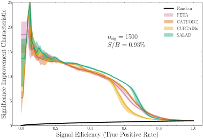
Figure 2: Significance Improvement Characteristic for a binary classifier trained to discriminate each synthetic background generation method’s samples from signal-contaminated data. Below this signal injection ($n_{\mathrm{sig}}=1500$), methods perform less equally. For readability, we withhold a description of the classifier architectures and ensembling choices until Sec. 2.3.

2.2 Dataset

We use the LHC Olympics 2020 R&D dataset LHCOlympics ; Kasieczka:2021xcg , which consists of 1,000,000 background events comprised of QCD dijet production, together with 100,000 signal events from a $Z^{\prime}$ resonance at 3.5 TeV, decaying to scalars $X$ and $Y$ at 500 GeV and 100 GeV respectively, which then each decay to quark pairs. Since the $X$ and $Y$ scalars are highly boosted, their decay products are highly collimated and form large-radius jets. For the main resonant feature, we use the dijet invariant mass ($m=m_{JJ}$) which should reconstruct the $Z^{\prime}$ mass for the signal. Events are required to have at least one large-radius anti-$k_{T}$ Cacciari:2011ma ; Cacciari:2008gp jet ($R=1$) with a $p_{T}$ threshold of $1.2$ TeV. Each event contains up to 700 particles with three degrees of freedom $p_{T}$, $\eta$, $\phi$. The events are generated with Pythia 8.219 Sjostrand:2006za ; Sjostrand:2014zea and Delphes 3.4.1 deFavereau:2013fsa . Also included in the LHC Olympics dataset is a set of 1,000,000 Herwig++B_hr_2008 QCD dijet events generated using the same tunes, which is used for the simulation-assisted approaches (SALAD and FETA) as the auxiliary “simulated” data (SIM). We therefore denote the Pythia events as “data” (DAT).

In addition to the LHC Olympics dataset, we make use of two auxiliary sets of QCD dijet events generated using the same tunes as the LHC Olympics dataset, but only in the $m_{JJ}$ region [3.3, 3.7] TeV (our chosen signal region). The first set, consisting of 1,000,000 Herwig++-based events, is used to generate additional SALAD samples. The second set, consisting of 320k Pythia-based events, is used for testing the synthetic samples.

We choose a feature space of six dijet observables $m_{J_{1}}$, $\Delta m_{JJ}$, $\tau^{21}_{J_{1}}$, $\tau^{21}_{J_{2}}$, $\Delta R_{JJ}$, and $m_{JJ}$ (see Figs. 3 and 4). This last feature is our mass-like event variable, which we use to define a SR spanning [3.3, 3.7] TeV. For our sidebands, we use the full amount of available data, down to 1.5 TeV and up to 5.5 TeV.

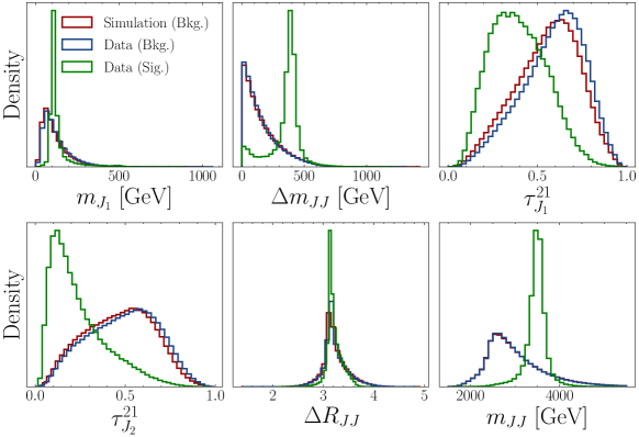
Figure 3: The 5-dimensional feature space of dijet collision events used in this resonant AD study. We also show a 6th feature, a mass-like event variable that is used to define a signal region (SR) and sidebands regions (SB).

Synthetic samples are generated using the procedure outlined in each method’s respective paper. However, in an attempt to equalize the quality of the samples as much as possible, all methods are given the same training and validation sets of simulation and data, which is an 80-20 split of the full sidebands data, i.e. all data in the range ([1.5, 5.5] $\setminus$ [3.3, 3.7]) TeV. These training and validation event counts, as well as the number of synthetic SM samples generated for each method, are shown in Table 2.

The CATHODE, CURTAINs, and FETA methods all involve training a generative model (i.e. a normalizing flow) to learn an underlying probability distribution. This allows us to reduce statistical uncertainties of the synthetic SM samples by oversampling from the generative models. For CATHODE, we can sample from the normalizing flow that has been interpolated into the SR as many times as we want; for CURTAINs (or FETA), we can similarly oversample from the normalizing flows that learn the densities of SB data (or SR simulation). In this study, we use the oversampling factor (also shown in Table 2) that was shown to saturate each model’s performance in its respective paper.

Method	Training data	Validation data	# samples	Oversampling
SALAD	793k SIM, 696k DAT	198K SIM, 174K DAT	1,045k	N/A
CATHODE	696k DAT	174K DAT	400k	3
CURTAINs	373k DAT	93k DAT	1,887k	4
FETA	793k SIM, 696k DAT	198K SIM, 174K DAT	732k	6

Table 2: Numerical breakdown of the events used to construct the given number of synthetic SM samples (in the SR) for the four machine learning methods considered in this report. The CURTAINs method uses a slightly narrower SB region of [2.7, 4.5] TeV to avoid transforming events across the $m_{JJ}$ turn-on region border. The SALAD samples are generated by applying the learned weights to an additional, much larger set of Herwig++ simulated SM events not contained in the LHC Olympics dataset. Note that CATHODE and CURTAINs are data-exclusive (i.e. fully data-driven), using only the the “detected” (DAT) Pythia set, while SALAD and FETA require an auxiliary “simulated” (SIM) Herwig++ set.

2.3 Classifier architecture

As stated earlier, a set of synthetic SM background samples can be used for a resonant AD task by training a binary classifier to discriminate the samples from a set of detected SR data. If the SR data contains a nonzero percentage of BSM events, then the binary classifier should be able to pick up on this difference. In fact, that classifier (in the limit of infinite data and arbitrarily flexible training / architecture) is the optimal one for distinguishing SM background from the BSM signal Metodiev:2017vrx .

Concretely, the discrimination task in this paper is between a given method’s synthetic SM samples and a set of 121k SR DAT background + $n_{\mathrm{sig}}$ SR DAT signal ($Z^{\prime}$) events, where $n_{\mathrm{sig}}$ is a controllable parameter, the number of injected signal events in the SR.

To evaluate the similarity between two datasets of events, we use a binary classifier network consisting of 3 linear layers of size (64, 32, 1). The network uses rectified linear unit (ReLU) activations and is optimized using Adam adam on the Binary Cross Entropy loss. We train using a 5-fold cross validation scheme, keeping the network with the best validation loss. Each fold is trained with a batch size of 128 and a learning rate of $10^{-3}$ for up to 100 epochs with a patience of 5 epochs. All hyperparameters were optimized via manual tuning to give the best possible significance improvement characteristic curves (introduced formally in Sec. 4). All errorbars and errorbands in plots come from retraining the binary classifier with different random seeds. Note that we do not explicitly study the effect of varying the random seeds for training the architectures that generate each set of synthetic samples. We believe that this variation would have an effect similar in magnitude to that of the binary classifier seed variation, but we leave it to future work to explore.

All figures and summary statistics are generated by evaluating the relevant trained binary classifier network on a “standard test set” of 20,000 signal and 320,000 background dijet events, which are not used at any time during the training procedure. Using a larger number of background events for evaluation allows for smooth summary statistics at low signal efficiencies, which is expected to be the relevant region for resonant AD. Unless explicitly stated otherwise, all plots are score-averaged for each method, i.e. the plots are derived from the average of classifier scores over 10 independent runs.

3 Contrasting the synthetic SM samples

3.1 Background-only case

As a first test of the synthetic SM samples created by each of the four generation methods, we compare their distributions to background-only SM data, i.e. with a signal injection $n_{\mathrm{sig}}=0$. These distributions are shown in Fig. 4. We see that at this level all four methods reproduce the true distribution well.

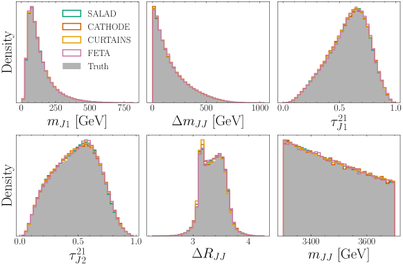
Figure 4: Distributions of synthetic SM backgrounds generated by each method compared to data with $n_{\mathrm{sig}}=0$.

As a next text of the synthetic SM samples created by each of the four generation methods, we analyze classifiers trained to discriminate synthetic SM background from background-only SM data, i.e. with a signal injection $n_{\mathrm{sig}}=0$. Given that there is no BSM signal present in the training data, differences in classifier performances come down to the “nature” of the synthetic SM samples for each method. All of the methods are given the same training and validation data sets, so the statistical fluctuations from the input data should be correlated between methods. Further, all of the binary classifiers are evaluated with the same random seed, so the network initializations should be identical in that respect. However, there are differences stemming from the initialization of the neural networks for each method, as well as from the differences of the methods themselves. These differences might be expected to decorrelate the classifier scores.

We provide the receiver operating characteristic area-under-the-curves (AUC) for such classifiers in Fig. 5. Interestingly, AUCs for all such methods are only just non-consistent with 0.5, which would correspond to a random classifier.

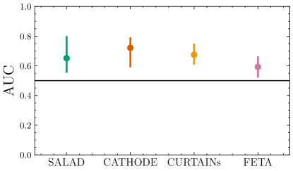
Figure 5: Receiver operating characteristic area-under-the-curves (AUC) for binary classifiers trained to discriminate each method’s synthetic samples from data with $n_{\mathrm{sig}}=0$. The table summarizes 100 classifier runs with different random seeds, with errorbars showing a 68-percentile spread. No score averaging has been done for this plot.

Figure 6 plots the classifier scores, averaged over 10 classifier runs, as evaluated on the test set’s background events. Note that we plot the standardized scores, since the binary classifier is trained to flag the most anomalous events with the highest scores. We also focus on the first quadrant of the coordinate plane, corresponding to the“anomaly regions” of the plots, or the highest regions in (standardized) score space where the classifier-flagged anomalies are expected to lie. In general, the classifier scores for the networks trained to discriminate detected data from each synthetic sample generation method do not appear to agree across methods: the scores are, for the most part, uncorrelated when evaluated on true background events.

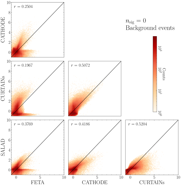
Figure 6: Scores for background events for a binary classifier trained to discriminate synthetic SM background from data with $n_{\mathrm{sig}}=0$). Each axis represents a different method of SM sample generation. $r$ denotes the Pearson correlation coefficient. The scores are standardized so as to make it clear what events the binary classifier flags as the most anomalous. For each method, scores are averaged over 10 classifier runs.

As a next task, we quantify the similarity across sample generation methods of events that are deemed “signal-like” by the binary classifier. As our similarity metric, we consider the background events in the standard test set with classifier scores in the top $p$ percentile, i.e. the background events classified as the most “signal-like”, or most different to the synthetic background samples. Within the scope of an anomaly detection search, these top $p$-percentile events are exactly those that correspond to high-score, likely-to-be-anomalous events.

For each percentile $p$, we find the set of the top $p$ events independently for the classifiers trained on all four methods. We then calculate the overlaps between the sets of selected events between each pair of sample generation methods, then across all four methods. Note that for fully independent event selection methods, we would expect a fraction $p$ of shared events by chance; therefore for easier visualization, we plot the excess overlap with respect to this random baseline in Fig. 7 (subtracting the correct baseline for the overlap of all four methods). If the excess overlap is 0, then the performance overlap is no more than expected by random chance.

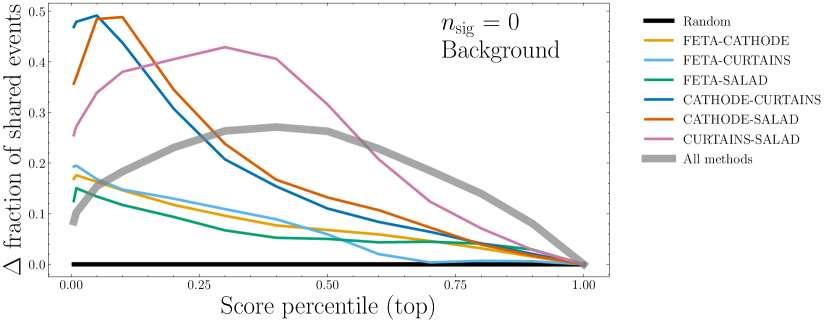
Figure 7: Fractional overlap, with respect to a random-choice baseline, of the $p$th percentile of true background events classified as the most “signal-like” between different methods of synthetic SM sample generation. For each method, scores are averaged over 10 classifier runs.

For most combinations of synthetic sample generation methods, the amount of overlap between any two sample generation methods is slightly greater than what we would expect between two uncorrelated sets of random numbers, especially for larger score percentiles. However, there appears to be a large amount of similarity between CATHODE and SALAD, and between CATHODE and CURTAINs, especially at small percentiles. There is also large degree of similarity between CURTAINs and SALAD, especially at larger percentiles.

Another way to study the quality of the background-only samples relative to each other utilizes a multiclass classifier. This method of comparing different generative models was first introduced in Lim:2022nft in the context of up-sampling hydrodynamical galaxy simulations. (See also Diefenbacher:2023vsw for a subsequent application to comparing generative models for fast calorimeter simulation.) We use the same classifier architecture as before and only modify the output layer to yield 4 (softmaxed) numbers, which we interpret as the probabilities of the input samples belonging to one of the four methods. We also use a larger batch size of 1000, which we found necessary in order to get repeatable results. We use a subset of 400,000 samples from each of the four methods to train (60%), test (20%), and evaluate (20%) the classifier. Samples from SALAD get their appropriate sample weight in training, testing, and evaluation. Since the average of these weights is about 0.98, we add an additional class weight of 1/0.98 = 1.021 to the SALAD samples to correct for the small imbalance.

For final evaluation and comparison of the samples, we consider the average of the log posterior Lim:2022nft , which is defined as

$$LP(\text{model }i|\text{samples }j)=\frac{1}{N}\sum_{x_{k}\in j}\omega_{k}\log{p_{\text{model }i}(x_{k})},$$ (1)

evaluated on the held-out test datasets. Here, the sum includes all samples $x_{k}$ of the tested model $j\in$ (SALAD, CATHODE, CURTAINs, FETA), $\omega_{k}$ is the sample weight of the sample $x_{k}$, and $N$ is the number of samples in the set. Since individual runs tend to scatter, we average the log posteriors over 100 independent classifier trainings with different random seeds. A well-trained multiclass classifier should be able to identify the samples belonging to each model, therefore we would expect to have

$$LP(\text{model }i|\text{samples }j=i)>LP(\text{model }i|\text{samples }j\neq i).$$ (2)

Indeed, this is what we observe in the first four columns of Fig. 8. The probability of belonging to a given model is highest for samples that were generated with that model for SALAD, CATHODE, CURTAINs (albeit only slightly for the latter two), and FETA. These results are consistent with the previous similarity studies: SALAD, CATHODE, and CURTAINs exhibit an above-average degree of similarity with each other, while FETA appears to be more independent. To assess the question which of the methods produces artificial background closest to “truth” (the true SR background SM events), we evaluate the log posterior of Eq. (1) for samples from the truth dataset. We see in the right column of Fig. 8 that all four methods are essentially of equivalent quality, with their log posterior scores all well within each other’s error bars.

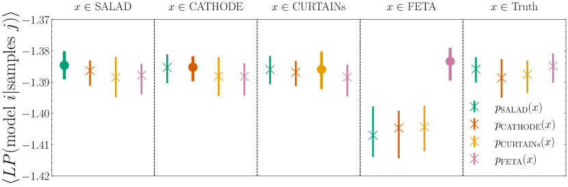
Figure 8: Average log posteriors $\langle LP(\text{model }i|\text{samples }j)\rangle$ of the multiclass classifier. The circle markers highlight the case $i=j$, and the cross markers indicate the cases $i\neq j$. “Truth” designates the SR SM background events. Errorbars show a 68-percentile spread of the $LP$s of 100 independent retrainings (no score averaging is carried out).

3.2 Adding in signal

In Figs. 9 and 10, we provide the scatterplots of the classifier scores evaluated on true background and true signal (respectively) events across different methods, this time for the case with injected signal: $n_{\mathrm{sig}}=1500$ ($S/B=0.93\%,S/\sqrt{B}=3.24$). Note that we fully retrain all classifiers for this new signal injection.

As shown in Fig. 9, for this larger signal injection (as compared with 0 signal injection in Fig. 6), the correlation between classifier scores for background events across synthetic sample generation method is somewhat higher, especially for correlations involving SALAD or FETA. In contrast, Fig. 10 shows that the classifier scores for signal events are highly correlated between any two methods; all methods seem to agree on what anomalous events are. To summarize these results: we see that the classifier scores are rather uncorrelated on background events, but highly correlated on signal events. This might mean that the characteristics (i.e. the 5-dimensional non-mass feature space) of the synthetic background that is created differ non-trivially from method to method; there isn’t overwhelming consensus on how to classify true background. However, all four of the methods produce background that is non-trivially different from true signal, at least different enough that classifiers can reliably distinguish background from signal.

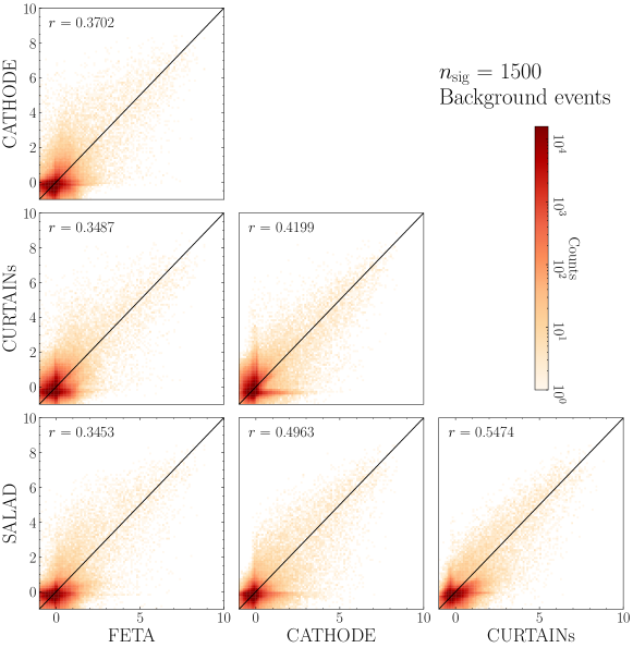
Figure 9: Scores for background events for a binary classifier trained to discriminate synthetic SM background from data with $n_{\mathrm{sig}}=1500$, $S/\sqrt{B}$ = 3.24). Each axis represents a different method of SM sample generation.

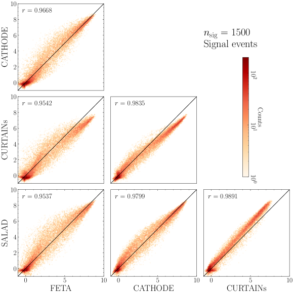
Figure 10: Scores for signal events for a binary classifier trained to discriminate synthetic SM background from data with $n_{\mathrm{sig}}=1500$, $S/\sqrt{B}$ = 3.24). Each axis represents a different method of SM sample generation.

In Fig. 11, we once again plot the overlaps of the top-$p$ percentile most “signal-like” events for a training signal injection of $n=1500$. For background events (Fig. 11(a)), there is now a sizable amount of overlap between all pairs of methods at $p\lesssim 0.1$, though the overlap drops off quickly for larger percentiles. For the signal events (Fig. 11(b)), there is a significant excess of event overlaps between any two methods down to low-to-mid percentiles. This agrees with intuition: the natures of the synthetic SM samples may differ from method to method, but the hope is that they all differ significantly from a BSM resonance such that they can be used as a suitable background against which to discriminate the resonance. Importantly, there is an excess in event overlaps above random chance between all four methods across the board, at all percentiles.

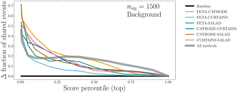
(a) True background events.

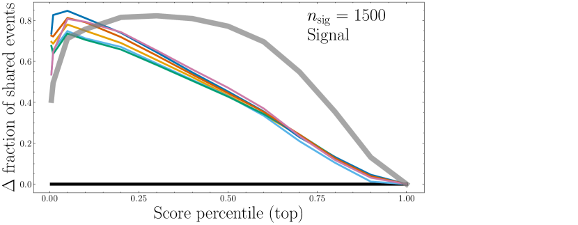
(b) True signal events.

Figure 11: Fractional overlap, with respect to a random-choice baseline, of the $p$th percentile of events classified as the most “signal-like” between different methods of synthetic SM sample generation.

In Fig. 12, we consider a slightly different view of the percentile overlaps by fixing the percentile of the most “signal-like” events and plotting this as a function of $n_{\mathrm{sig}}$ in the classifier training set. For the top 5 percentile of the most signal-like true background events, there appears to be slightly increasing similarity with the number of injected signal events $n_{\mathrm{sig}}$ across all four methods, but not between any two methods. For the top 5 percentile of the most signal-like true signal events, the agreement increases with $n_{\mathrm{sig}}$, leveling out at $n_{\mathrm{sig}}\approx 1200$. Put another way, the four methods considered here agree on what the 5% most anomalous events are when trained to discriminate their own synthetic SM samples from a dataset containing signal injections as low as 0.62%.

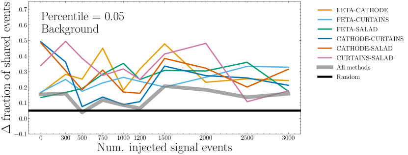
(a) True background events.

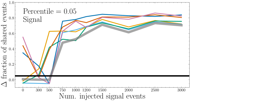
(b) True signal events.

Figure 12: Fractional overlap, with respect to a random-choice baseline, of the 5th percentile of events classified as the most “signal-like” between different methods of synthetic SM sample generation, scanning over $n_{\mathrm{sig}}$.

4 Combining the samples

In this section, we investigate the amount which combining the synthetic samples can provide a more faithful approximation for SM background than taking samples from any of the individual generation methods alone. We have seen previously that classifiers trained to discriminate an individual method’s synthetic samples from data tend to agree on what anomalous, signal-like events are more often than random. However, the agreement isn’t absolute. This might indicate that the events that each method’s classifier are flagging as anomalous occupy slightly different parts of phase space. Therefore by combining the synthetic samples, we could hope to be more broadly sensitive to a larger phase space.

There are numerous ways to combine the sample generation methods, as the combination can in principle be done at one of many stages of an analysis. Additionally, one could imagine combining methods in a way that prioritizes one method over the other three. In this section, we will investigate the two most straightforward combinations that weight all four methods in the same way: first at the sample level, and second at the (classifier) score level.

To combine generation methods at the sample level, we take 250k samples from each method so that each contributes equally. We then train a binary classifier to discriminate the combined synthetic samples from the SR data, varying $n_{\mathrm{sig}}$ from 0 to 3000 (corresponding to $S/B$ in the SR of $0\%$ to $1.86\%$). We evaluate each classifier on the standard test set. To combine generation methods at the score level, we simply average the score given to a given test set event over each of the four methods.

To aggregate classifier runs, we train 100 such binary classifiers, average scores across ensembles of 10 runs, and generate classifier metric curves using the ensembled scores. This has the effect of tightening the errorbands for Figs. 13 and 14, making them easier to parse.

In Fig. 13, we provide summary plots across the range of tested $n_{\mathrm{sig}}$ values. In Fig. 13(a), we calculate the classifier significance improvement characteristic (SIC) as a function of the signal efficiency, then take the maximum of the SIC. The max(SIC) gives the best multiplicative improvement to signal significance, corresponding to the best-motivated cut (which we do not know a priori). In Fig. 13(b), we plot the significance at a background rejection of $10^{3}$, which is less sensitive to the low-signal efficiency fluctuations of the max(SIC). Based on these metrics, the combined synthetic samples are competitive with, but not necessarily better than, any of the individual sample generation methods. In particular, SALAD looks to be the method to beat at the majority of signal injections.

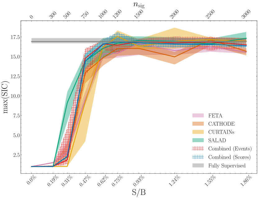
(a) Maximum of the Significance Improvement Characteristic.

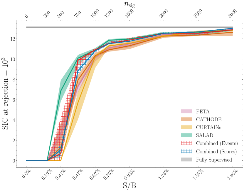
(b) Significance Improvement Characteristic at a classifier rejection of $10^{3}$.

Figure 13: Various metrics for a classifier trained to discriminate a combination of FETA, CATHODE, and CURTAINs synthetic SM samples from data over a range of $n_{\mathrm{sig}}$ values. Errorbands show a 68-percentile spread across the median and come from training a 5-fold classifier 100 times with different random seeds and ensembling scores over 10 runs.

However, the summary statistics alone may not be the most helpful gauge for performance in an AD task, since we do not necessarily know the cut value corresponding to the max(SIC). In Fig. 14, we provide additional summary plots for the lowest signal injection $n_{\mathrm{sig}}=750$ ($S/B=0.74\%$) where using the combined samples leads to an improvement over using any individual method. While the two combination methods (i.e. at the sample and score levels) are comparable, the sample-level combination does appear to give better performance at most signal efficiencies.

Based on these plots, using the combined samples as the SM background leads to a classifier that is uniformly better (with respect to signal efficiency) at detecting the small amount of signal. This implies that when the score cutoff corresponding to the max(SIC) is unknown — as it is in virtually all AD tasks — combining synthetic SM samples is the optimal strategy.

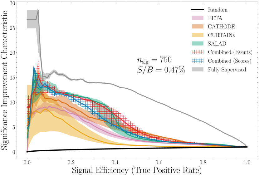
(a) Significance Improvement Characteristic plotted against the signal efficiency.

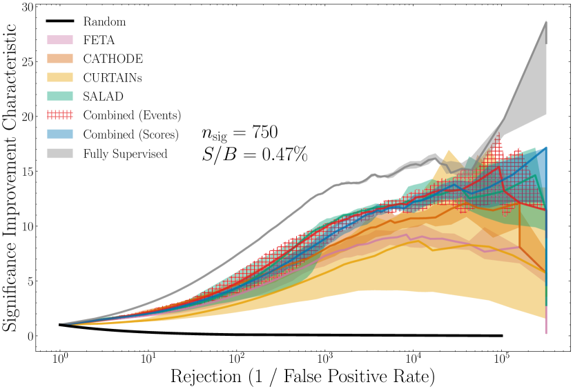
(b) Significance Improvement Characteristic plotted against classifier rejection.

Figure 14: Various classifier metrics for a classifier trained to discriminate a combination of FETA, CATHODE, and CURTAINs synthetic SM samples from data with $n_{\mathrm{sig}}=750$. Errorbands show a 68-percentile spread across the median and come from training a 5-fold classifier 100 times with different random seeds, ensembling scores over 10 runs, and averaging classifier metrics over the ensembles.

5 Conclusions

In this paper, we have explored four conceptually different methods of generating synthetic Standard Model (SM) background samples to be used for resonant anomaly detection (AD) tasks: SALAD, CATHODE, CURTAINs, and FETA. Each method uses a different means of generating a set of synthetic Standard Model samples to be used as a background set for resonant anomaly detection, but all use the same meta-format: shift in some way a sample of background-only events (pulled from an auxiliary dataset or background-only regions in data) to a signal region of interest, and search for a resonant anomaly within that region, such as by estimating an anomaly score based on the data-to-background likelihood ratio in non-$m$ features and cutting on it to enhance on the standard bump hunt procedure.

In general, the four construction methods produce synthetic SM samples that perform similarly when used for resonant AD tasks. Binary classifiers trained to discriminate SM samples from SALAD, CATHODE, CURTAINs, and FETA against data (SM background + injected signal) assign scores to the signal events that are generally correlated. Furthermore, the four methods agree on what the top $p$ percentile of the most “signal-like” events are. While all methods perform similarly on their own with respect to being able to detect evidence of anomalous events as quantified by their max(SICs), combining the four methods allows for a more sensitive AD tool at any given signal efficiency. This is especially useful in practice, when we do not know the optimal score cutoff corresponding to the max(SIC). We find that there is enough evidence to recommend that future AD tasks make use of this combined strategy for generating synthetic SM background samples.

With an eye towards future work: the LHC Olympics dataset is used as a benchmarking tool in the majority of resonant AD R&D, but it represents just one resonant anomaly type out of a vast landscape. It is very possible that the results found in this report do not perfectly extend to other BSM particles. In that respect, it is interesting to remember the background (SM) -only studies in Sec. 3.1, which showed that the four methods considered in this work do seem to produce samples that cover non-overlapping regions of phase space. It would also be useful to consider other means of combining the synthetic samples, perhaps at the level of classifier metrics other than at the event-level or score-level, or in ways that prioritize one method in particular.

Code avalability

All analysis code can be found at https://github.com/rmastand/synthetic_SM_AD/tree/main.

Appendix A Robustness of classifier scores

One might hope that the nature of the synthetic samples produced by each of the four generation methods considered in this report are robust in the sense that they consistently produce the same results despite variances in the binary classifier initialization and training procedure. To gauge this robustness, in Fig. 15, we plot the classifier scores derived from samples of the same method, but for classifiers trained starting with a different random seed, all on background-only events ($n_{\mathrm{sig}}=0$).

These plots illustrate that the scores output by the random classifier are relatively robust with respect to the training procedure when trained on a single sample generation method: the correlation between different random seeds is greater than 90% for all methods. However, in the main text of this paper, we elect to show results derived from scores averaged over 10 classifier trials (i.e. with different random seeds). This choice helps to stabilize the results, such that we are not comparing an uncharacteristically good classifier run for one method with an uncharacteristically bad classifier run for another.

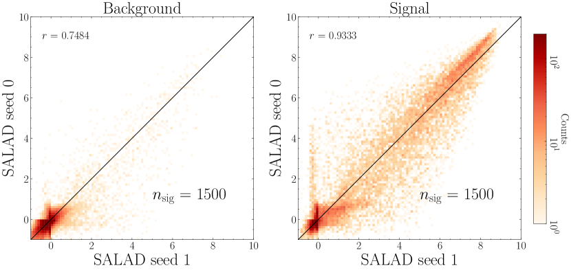
(a) SALAD against SALAD.

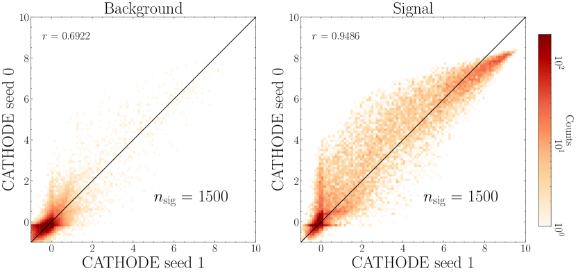
(b) CATHODE against CATHODE.

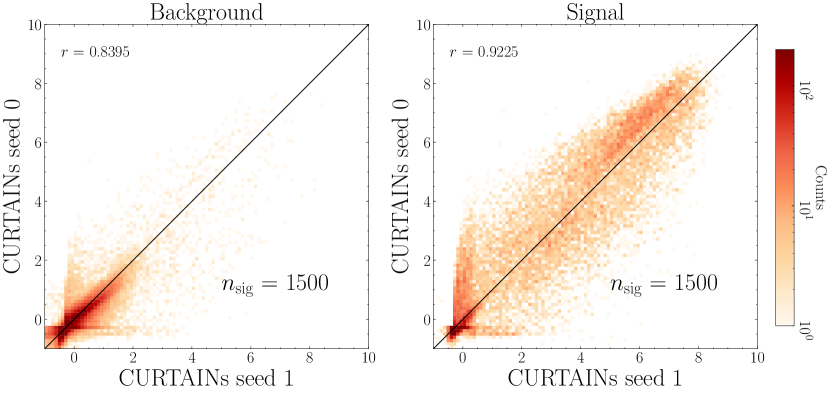
(c) CURTAINs against CURTAINs.

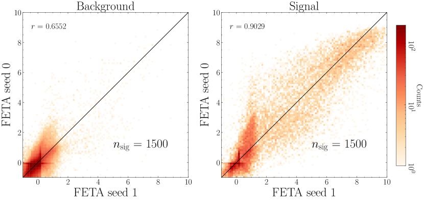
(d) FETA against FETA.

Figure 15: Classifier scores for a binary classifier trained to discriminate synthetic SM background from data with $n_{\mathrm{sig}}=1500$). Each axis represents a different random seed for the same sample generation method.

Appendix B Additional plots

In this section, we provide a small number of supplementary plots to complement the main text figures. In Fig. 16, we plot the standardized scores for true signal events, as calculated by a binary classifier trained to discriminate the synthetic samples from data with $n_{\mathrm{sig}}=0$. This is a companion plot to Fig. 6. In Fig. 17, we plot the fractional overlap, with respect to a random-choice baseline, of the $p$th percentile of true signal events classified as the most “signal-like” between different methods of synthetic SM samples. This is a companion plot to Fig. 7.

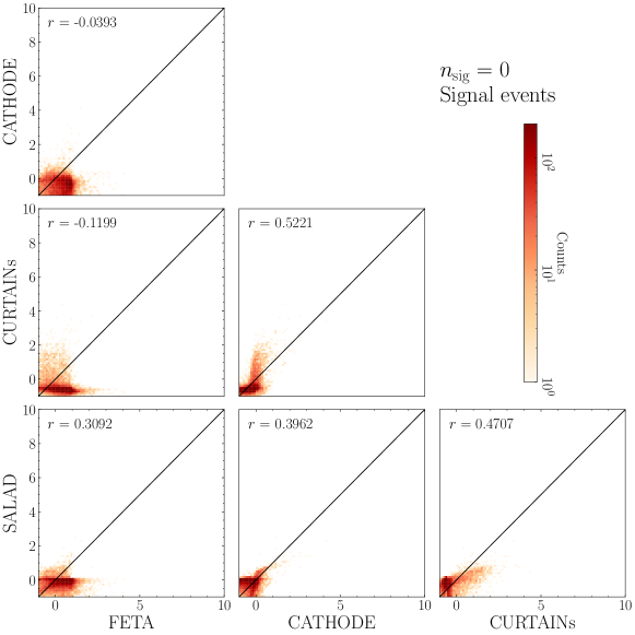
Figure 16: Scores for signal events for a binary classifier trained to discriminate synthetic SM background from data with $n_{\mathrm{sig}}=0$). Each axis represents a different method of SM sample generation. $r$ denotes the Pearson correlation coefficient. The scores are standardized so as to make it clear what events the binary classifier flags as the most anomalous. For each method, scores are averaged over 10 classifier runs. This is a companion plot to Fig. 6

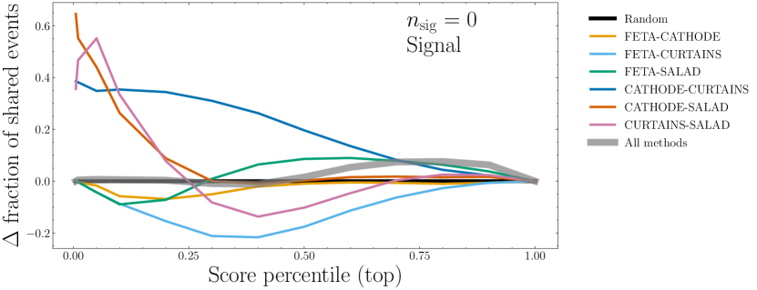
Figure 17: Fractional overlap, with respect to a random-choice baseline, of the $p$th percentile of true signal events classified as the most “signal-like” between different methods of synthetic SM sample generation. For each method, scores are averaged over 10 classifier runs. This is a companion plot to Fig. 7.

References

- (1) ATLAS Collaboration, G. Aad et al., “Observation of a new particle in the search for the Standard Model Higgs boson with the ATLAS detector at the LHC,” Phys. Lett. B 716 (2012) 1–29, arXiv:1207.7214 [hep-ex].
- (2) CMS Collaboration, S. Chatrchyan et al., “Observation of a New Boson at a Mass of 125 GeV with the CMS Experiment at the LHC,” Phys. Lett. B 716 (2012) 30–61, arXiv:1207.7235 [hep-ex].
- (3) ATLAS Collaboration, “Exotic Physics Searches,” 2019. https://twiki.cern.ch/twiki/bin/view/AtlasPublic/ExoticsPublicResults.
- (4) ATLAS Collaboration, “Supersymmetry searches,” 2019. https://twiki.cern.ch/twiki/bin/view/AtlasPublic/SupersymmetryPublicResults.
- (5) ATLAS Collaboration, “Higgs and Diboson Searches,” 2019. https://twiki.cern.ch/twiki/bin/view/AtlasPublic/HDBSPublicResults.
- (6) CMS Collaboration, “CMS Exotica Public Physics Results,” 2019. https://twiki.cern.ch/twiki/bin/view/CMSPublic/PhysicsResultsEXO.
- (7) CMS Collaboration, “CMS Supersymmetry Physics Results,” 2019. https://twiki.cern.ch/twiki/bin/view/CMSPublic/PhysicsResultsSUS.
- (8) CMS Collaboration, “CMS Beyond-two-generations (B2G) Public Physics Results,” 2019. https://twiki.cern.ch/twiki/bin/view/CMSPublic/PhysicsResultsB2G.
- (9) LHCb Collaboration, “Publications of the QCD, Electroweak and Exotica Working Group,” 2019. http://lhcbproject.web.cern.ch/lhcbproject/Publications/LHCbProjectPublic/Summary_QEE.html.
- (10) G. Karagiorgi, G. Kasieczka, S. Kravitz, B. Nachman, and D. Shih, “Machine Learning in the Search for New Fundamental Physics,” arXiv:2112.03769 [hep-ph].
- (11) G. Kasieczka et al., “The LHC Olympics 2020 a community challenge for anomaly detection in high energy physics,” Rept. Prog. Phys. 84 no. 12, (2021) 124201, arXiv:2101.08320 [hep-ph].
- (12) T. Aarrestad et al., “The Dark Machines Anomaly Score Challenge: Benchmark Data and Model Independent Event Classification for the Large Hadron Collider,” SciPost Phys. 12 no. 1, (2022) 043, arXiv:2105.14027 [hep-ph].
- (13) ATLAS Collaboration, G. Aad et al., “Anomaly detection search for new resonances decaying into a Higgs boson and a generic new particle in hadronic final states using TeV collisions with the ATLAS detector,” arXiv:2306.03637 [hep-ex].
- (14) ATLAS Collaboration, “Search for new phenomena in two-body invariant mass distributions using unsupervised machine learning for anomaly detection at TeV with the ATLAS detector,” tech. rep., CERN, Geneva, 2023. https://cds.cern.ch/record/2859329. All figures including auxiliary figures are available at https://atlas.web.cern.ch/Atlas/GROUPS/PHYSICS/CONFNOTES/ATLAS-CONF-2023-022.
- (15) J. H. Collins, K. Howe, and B. Nachman, “Anomaly Detection for Resonant New Physics with Machine Learning,” Phys. Rev. Lett. 121 no. 24, (2018) 241803, arXiv:1805.02664 [hep-ph].
- (16) J. H. Collins, K. Howe, and B. Nachman, “Extending the search for new resonances with machine learning,” Phys. Rev. D99 no. 1, (2019) 014038, arXiv:1902.02634 [hep-ph].
- (17) A. Andreassen, B. Nachman, and D. Shih, “Simulation Assisted Likelihood-free Anomaly Detection,” Phys. Rev. D 101 no. 9, (2020) 095004, arXiv:2001.05001 [hep-ph].
- (18) B. Nachman and D. Shih, “Anomaly Detection with Density Estimation,” Phys. Rev. D 101 (2020) 075042, arXiv:2001.04990 [hep-ph].
- (19) K. Benkendorfer, L. L. Pottier, and B. Nachman, “Simulation-assisted decorrelation for resonant anomaly detection,” Phys. Rev. D 104 no. 3, (2021) 035003, arXiv:2009.02205 [hep-ph].
- (20) G. Stein, U. Seljak, and B. Dai, “Unsupervised in-distribution anomaly detection of new physics through conditional density estimation,” in 34th Conference on Neural Information Processing Systems. 12, 2020. arXiv:2012.11638 [cs.LG].
- (21) O. Amram and C. M. Suarez, “Tag n’ train: a technique to train improved classifiers on unlabeled data,” Journal of High Energy Physics 2021 no. 1, (Jan, 2021) . https://doi.org/10.1007%2Fjhep01%282021%29153.
- (22) A. Hallin, J. Isaacson, G. Kasieczka, C. Krause, B. Nachman, T. Quadfasel, M. Schlaffer, D. Shih, and M. Sommerhalder, “Classifying anomalies through outer density estimation,” Phys. Rev. D 106 no. 5, (2022) 055006, arXiv:2109.00546 [hep-ph].
- (23) J. F. Kamenik and M. Szewc, “Null hypothesis test for anomaly detection,” Phys. Lett. B 840 (2023) 137836, arXiv:2210.02226 [hep-ph].
- (24) A. Hallin, G. Kasieczka, T. Quadfasel, D. Shih, and M. Sommerhalder, “Resonant anomaly detection without background sculpting,” arXiv:2210.14924 [hep-ph].
- (25) M. F. Chen, B. Nachman, and F. Sala, “Resonant Anomaly Detection with Multiple Reference Datasets,” arXiv:2212.10579 [hep-ph].
- (26) T. Golling, S. Klein, R. Mastandrea, and B. Nachman, “Flow-enhanced transportation for anomaly detection,” Phys. Rev. D 107 no. 9, (2023) 096025, arXiv:2212.11285 [hep-ph].
- (27) D. Sengupta, S. Klein, J. A. Raine, and T. Golling, “Curtains flows for flows: Constructing unobserved regions with maximum likelihood estimation,” 2023.
- (28) ATLAS Collaboration, G. Aad et al., “Dijet resonance search with weak supervision using TeV collisions in the ATLAS detector,” Phys. Rev. Lett. 125 no. 13, (2020) 131801, arXiv:2005.02983 [hep-ex].
- (29) D. Shih, M. R. Buckley, L. Necib, and J. Tamanas, “Via Machinae: Searching for Stellar Streams using Unsupervised Machine Learning,” arXiv:2104.12789 [astro-ph.GA].
- (30) D. Shih, M. R. Buckley, and L. Necib, “Via Machinae 2.0: Full-Sky, Model-Agnostic Search for Stellar Streams in Gaia DR2,” arXiv:2303.01529 [astro-ph.GA].
- (31) M. Pettee, S. Thanvantri, B. Nachman, D. Shih, M. R. Buckley, and J. H. Collins, “Weakly-Supervised Anomaly Detection in the Milky Way,” arXiv:2305.03761 [astro-ph.GA].
- (32) E. M. Metodiev, B. Nachman, and J. Thaler, “Classification without labels: Learning from mixed samples in high energy physics,” JHEP 10 (2017) 174, arXiv:1708.02949 [hep-ph].
- (33) S. Choi, J. Lim, and H. Oh, “Data-driven Estimation of Background Distribution through Neural Autoregressive Flows,” arXiv:2008.03636 [hep-ph].
- (34) CMS Collaboration, “Evidence for the simultaneous production of four top quarks in proton-proton collisions at = 13 TeV,”.
- (35) G. Kasieczka, B. Nachman, and D. Shih, “Official Datasets for LHC Olympics 2020 Anomaly Detection Challenge (Version v6) [Data set].,” 2019. https://doi.org/10.5281/zenodo.4536624.
- (36) M. Cacciari, G. P. Salam, and G. Soyez, “FastJet User Manual,” Eur. Phys. J. C 72 (2012) 1896, arXiv:1111.6097 [hep-ph].
- (37) M. Cacciari, G. P. Salam, and G. Soyez, “The anti- jet clustering algorithm,” JHEP 04 (2008) 063, arXiv:0802.1189 [hep-ph].
- (38) T. Sjostrand, S. Mrenna, and P. Z. Skands, “PYTHIA 6.4 Physics and Manual,” JHEP 05 (2006) 026, arXiv:hep-ph/0603175.
- (39) T. Sjöstrand, S. Ask, J. R. Christiansen, R. Corke, N. Desai, P. Ilten, S. Mrenna, S. Prestel, C. O. Rasmussen, and P. Z. Skands, “An introduction to PYTHIA 8.2,” Comput. Phys. Commun. 191 (2015) 159–177, arXiv:1410.3012 [hep-ph].
- (40) DELPHES 3 Collaboration, J. de Favereau, C. Delaere, P. Demin, A. Giammanco, V. Lemaître, A. Mertens, and M. Selvaggi, “DELPHES 3, A modular framework for fast simulation of a generic collider experiment,” JHEP 02 (2014) 057, arXiv:1307.6346 [hep-ex].
- (41) M. Bähr, S. Gieseke, M. A. Gigg, D. Grellscheid, K. Hamilton, O. Latunde-Dada, S. Plätzer, P. Richardson, M. H. Seymour, A. Sherstnev, and B. R. Webber, “Herwig++ physics and manual,” The European Physical Journal C 58 no. 4, (Nov, 2008) 639–707. https://doi.org/10.1140%2Fepjc%2Fs10052-008-0798-9.
- (42) D. P. Kingma and J. Ba, “Adam: A method for stochastic optimization,” 2014. https://arxiv.org/abs/1412.6980.
- (43) S. H. Lim, K. A. Raman, M. R. Buckley, and D. Shih, “GalaxyFlow: Upsampling Hydrodynamical Simulations for Realistic Gaia Mock Catalogs,” arXiv:2211.11765 [astro-ph.GA].
- (44) S. Diefenbacher, E. Eren, F. Gaede, G. Kasieczka, C. Krause, I. Shekhzadeh, and D. Shih, “L2LFlows: Generating High-Fidelity 3D Calorimeter Images,” arXiv:2302.11594 [physics.ins-det].