Diffusion Models for Probabilistic Deconvolution of Galaxy Images

Abstract

Telescopes capture images with a particular point spread function (PSF). Inferring what an image would have looked like with a much sharper PSF, a problem known as PSF deconvolution, is ill-posed because PSF convolution is not an invertible transformation. Deep generative models are appealing for PSF deconvolution because they can infer a posterior distribution over candidate images that, if convolved with the PSF, could have generated the observation. However, classical deep generative models such as VAEs and GANs often provide inadequate sample diversity. As an alternative, we propose a classifier-free conditional diffusion model for PSF deconvolution of galaxy images. We demonstrate that this diffusion model captures a greater diversity of possible deconvolutions compared to a conditional VAE.

1 Introduction

High-fidelity galaxy models are important for deblending (Melchior et al., 2021), analyzing lens substructure (Mishra-Sharma & Yang, 2022), and validating the analysis of optical surveys (Korytov et al., 2019). Traditional galaxy models rely on simple parameteric profiles such as Sersic profiles (Sérsic, 1963). However, these models fail to capture the rich structures that are visible in modern surveys. As a result, there is growing interest in using deep generative models, such as variational autoencoders (VAEs), to represent galaxies (Regier et al., 2015; Castelvecchi, 2017; Lanusse et al., 2021).

Deep generative models of galaxies are fitted with images that have been observed with a particular point-spread function (PSF). It is thus necessary to account for the PSF in fitting these galaxy models, to disentangle the measurement process from the physical reality.

Because PSF convolution is not an invertible transformation, multiple deconvolved images are compatible with the observed image. Traditional deconvolution methods produce only one deconvolved image that is compatible with the image (Vojtekova et al., 2021). Deep generative models are an appealing alternative because they infer a distribution of deconvolved images that are compatible with an observation. Although conditional VAEs and conditional GANs (Schawinski et al., 2017; Fussell & Moews, 2019; Lanusse et al., 2021) can provide a distribution of deconvolved images, both are known to produce insufficient diversity in their outputs (Salimans et al., 2016).

Diffusion models are a recently developed alternative to VAEs and GANs that excel at producing diverse samples. Diffusion models have been successfully applied to solve inverse problems (Kawar et al., 2022; Remy et al., 2023; Adam et al., 2022; Song et al., 2022). However, training diffusion models with PSF convolved data to learn a representation of physical reality that is decoupled from the measurement process is not as straightforward as with a VAE. If we simply add a PSF convolution layer to the end of the diffusion model’s decoder, as we can with a VAE, training is no longer tractable.

Instead, we propose to model PSF-convolved galaxy images with a classifier-free conditional diffusion model (ho2021classifier) and to condition on the observed PSF. In training this model, we make use of paired data sources, e.g., both ground-based and space-based telescopes. We used a conditional VAE as a baseline and compared the methods using a novel evaluation method. We find that CVAEs tended to produce high percentages of invalid deconvolutions due to missing high-frequency details in reconstructions, resulting in lower sample diversity compared to conditional diffusion models. Our code is available from https://github.com/yashpatel5400/galgen

2 Methods

Let $x$ denote the observed (PSF-convolved) image, let $y$ denote the latent “clean” image, and let $\Pi$ denote the PSF. Then, neglecting pixelation and measurement noise, $x=\Pi*y$. We investigate classifier-free conditional diffusion models for solving the deconvolution task and we consider conditional VAEs as a baseline to compare against.

2.1 Conditional VAE

VAEs model the data distribution as a transformation of a lower-dimensional latent space (Kingma & Welling, 2013). An encoder $q_{\varphi}$ maps the input $x$ to a distribution over a low-dimensional latent expression $z$, which defines an approximate posterior distribution $q_{\varphi}(z\mid x)$; a decoder $p_{\theta}$ maps $z$ to the original data space through a generative model $p_{\theta}(x\mid z)$. Conditional VAEs (CVAEs) (Sohn et al., 2015) extend VAEs by conditioning both the encoder and decoder on auxiliary variables $c$, which may be denoted as $q_{\varphi}(z\mid x,c)$ and $p_{\theta}(x\mid z,c)$, respectively.

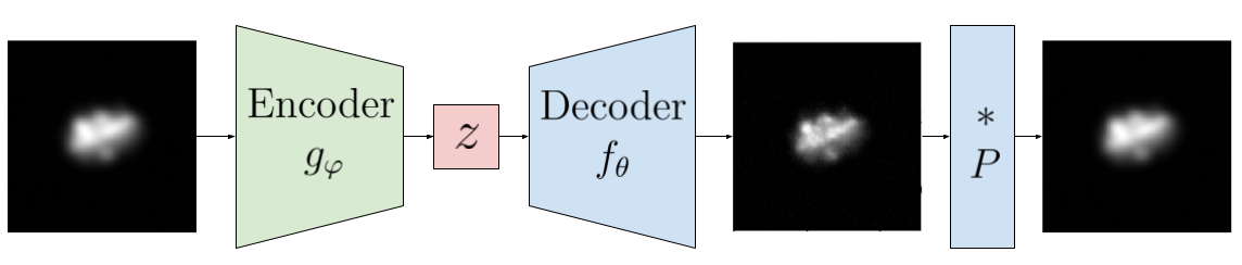
Figure 1: A CVAE is employed with a partially fixed decoder consisting of a deterministic convolution with the known PSF.

We investigate a CVAE in which $c=\Pi$ and the final layer of the decoder is fixed to be a convolution with the known PSF, as in Lanusse et al. (2021) and illustrated in Figure 1. With this approach, for each draw from the latent space, a candidate deconvolved image is produced as an intermediate result in the decoder, which is the quantity targeted by inference. For training, we take the loss to be a weighted-variant of the ELBO for the joint distribution $p(x,y\mid z)$:

$$\begin{gathered}\mathcal{L}_{\text{CVAE}}:=\alpha\ \mathbb{E}_{z\sim q_{\varphi}(z\mid x)}[\log(p_{\theta}(y\mid z))]\\ +\beta\ \mathbb{E}_{z\sim q_{\varphi}(z\mid x)}[\log(p_{\theta}(x\mid y,z))]\\ -D_{KL}(q_{\varphi}(z\mid x)||p_{\theta}(z)).\end{gathered}$$ (1)

Note that the first term targets the reconstruction of the deconvolved image. The hyperparameter weighting terms $\alpha$ and $\beta$ asymmetrically weight the PSF-convolved and deconvolved reconstructions, a formulation similar to the $\beta$-VAE (Higgins et al., 2017), which we found to improve the reconstruction of high-frequency details in samples.

2.2 Conditional Diffusion Models

Conditional diffusion models, an extension on denoising diffusion probabilistic models (Ho et al., 2020), are trained with the following loss function:

$$\mathcal{L}_{\text{Diff}}:=\mathbb{E}_{t\sim[1,T],\mathbf{x}_{0},\boldsymbol{\epsilon_{t}}}\left[||\boldsymbol{\epsilon}_{t}-\boldsymbol{\epsilon}_{\theta}(\mathbf{x}_{t},t,c)||^{2}\right],$$ (2)

where $\boldsymbol{\epsilon}_{\theta}(\mathbf{x}_{t},t,c)$ predicts the noise added to $\mathbf{x}_{t}$ (the latent variable for time step $t$) and $c$ is the conditioning information. We set $c=(x,\Pi)$. Therefore, at inference time, to deconvolve the image $x\in\mathbb{R}^{k_{1}\times k_{2}}$, a deconvolved image $y$ is sampled by first sampling $x_{0}\sim\mathcal{N}(0,I_{k_{1}k_{2},k_{1}k_{2}})$ and then taking $T$ denoising steps conditioned on $(x,\Pi)$.

2.3 Evaluation Metrics

Recent works such as Hackstein et al. (2023) have investigated metrics for the related task of generating galaxy images. However, the task of galaxy generation is distinct from ours, as we are seeking to produce diverse candidates conditional on a single observed image. Thus, simply measuring the recovery of the marginal distribution $p(y)$ of deconvolved images is insufficient to assess performance for our task. Furthermore, no paired reference data is available that provides observations of $x$ paired with multiple draws of $y$ for each $x$.

Instead, to assess the diversity of samples from the posterior $p(y\mid x,\Pi)$, we propose the following metric, where a given $q$ must satisfy the specified constraint:

$$\mathbb{E}_{x\sim p(x)}\left[\mathbb{V}_{y\sim q(y\mid x,\Pi)}[y]\right]$$ (3)

s.t. $$\mathbb{E}_{x\sim p(x)}\left[\mathbb{E}_{y\sim q(y\mid x,\Pi)}\left[||\Pi*y-x||_{2}^{2}\right]\right]<\epsilon.$$

Here, $\epsilon$ represents an allowed slack and $\mathbb{V}$ denotes the total variance of $y$ given both $x$ and $\Pi$. By adding the constraint, we ensure that high-scoring methods produce valid deconvolutions. To avoid favoring methods that generate images with imperceptible pixel-level variance, we compute $\mathbb{V}$ over image featurizations, defined by mapping the domain of images $\mathcal{Y}$ to image features $\mathcal{F}$ with a pre-trained InceptionV3 network; this idea is inspired by the Fréchet inception distance (FID). That is, for distributions $p(y\mid x)$ and $q(y\mid x)$ defined over the space of images, we fit two distributions, $\mathcal{N}(\mu^{(p)}_{y\mid x},\Sigma^{(p)}_{y\mid x})$ and $\mathcal{N}(\mu^{(q)}_{y\mid x},\Sigma^{(q)}_{y\mid x})$ respectively, over featurizations of the image space. Note that these distributions are fitted separately for each $x_{i}$ in a test collection $\{x_{i}\}_{i=1}^{N}$, giving a collection of distributions $\{\mathcal{N}(\mu^{(q)}_{y|x_{i}},\Sigma^{(q)}_{y|x_{i}})\}_{i=1}^{N}$. Finally, the objective is estimated as

$$\mathbb{E}_{x\sim p(x)}\left[\mathbb{V}_{y\sim q(y\mid x,\Pi)}[y]\right]\approx\frac{1}{N}\sum_{i=1}^{N}\text{Tr}\left(\Sigma^{(q)}_{y|x_{i}}\right).$$ (4)

3 Experiments

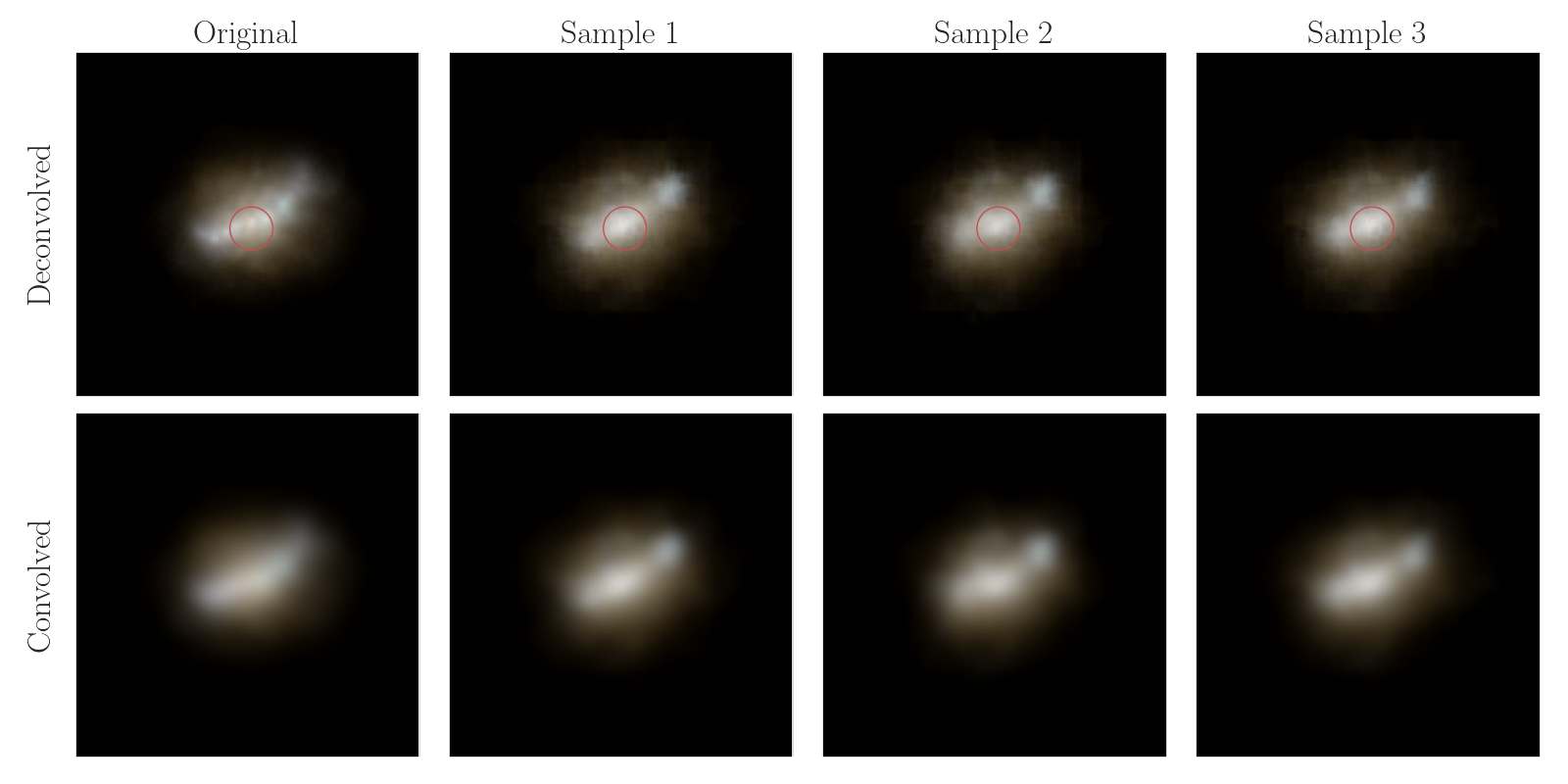
Figure 2: Candidate deconvolutions from the CVAE model. It can be seen that the generated samples shown are roughly valid inverse mappings by comparing them following convolution with the PSF (bottom row, columns 2–4) to the original PSF-convolved image (bottom row, column 1). However, high-frequency details, such as the belt of stars along the middle and other regions highlighted with red circles, are lost in reconstruction.

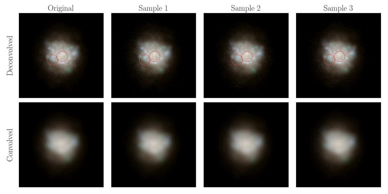
Figure 3: Candidate deconvolutions from the conditional diffusion model. It can be seen that the generated samples shown are roughly valid inverse mappings by comparing them following convolution with the PSF (bottom row, columns 2–4) to the original PSF-convolved image (bottom row, column 1). Additionally, high-frequency details (highlighted with red circles) are prominently captured in deconvolutions, enabling a greater diversity of reconstructions.

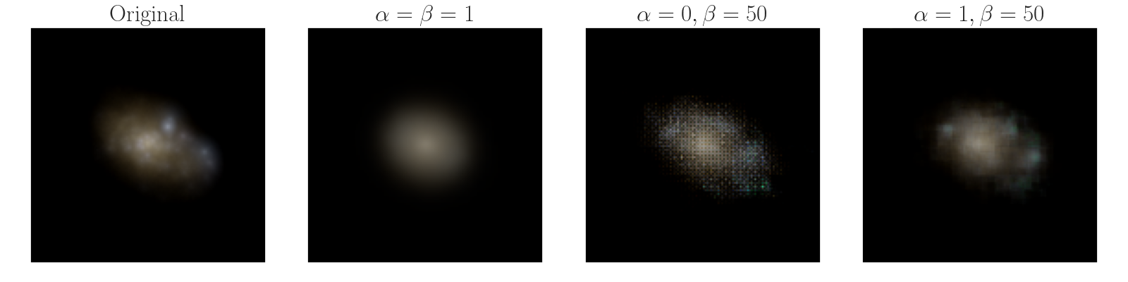
Figure 4: A representative sample from CVAEs trained to convergence with different choices of weights for the deconvolved and convolved image reconstructions, i.e. $\alpha$ and $\beta$ respectively. Observe that increasing the weight of the clean reconstruction tends to result in the loss of high-frequency detail.

We experiment with galaxy images produced by the IllustrisTNG simulator (Pillepich et al., 2018). This dataset provides a synthetic testbed similar in structure to the paired dataset of ground- and space-based telescope images that motivates our work. We construct a dataset consisting of tuples $\{(x_{i},y_{i},\Pi_{i})\}_{i=1}^{n}$ by convolving each clean image $y_{i}$ with a PSF $\Pi_{i}$ sampled from a collection. We view the use of the clean image $y_{i}$ as an idealized surrogate for space-based telescopes.

Our dataset consists of 9718 images, each $128\times 128$ pixels, with 7774 used for training and 1944 reserved for validation. Evaluation of the aforementioned FID-like and variance metrics was performed on the validation set. Note that inference does not use the clean images. PSFs were taken to be discretized two-dimensional isotropic Gaussians on grids of size $10\times 10$ with varying choices of $\sigma\in[2.0,4.0]$ discretized in intervals of 0.5.

All experiments were implemented in PyTorch (Paszke et al., 2019). A standard U-Net architecture was used for the DDPM denoiser $\boldsymbol{\epsilon}_{\theta}(\cdot)$. Our implementation of the DDPM was based on the “Conditional Diffusion MNIST” project (Pearce et al., 2022). Our CVAE employed a standard CNN-based architecture for both the encoder and decoder, with transposed convolutional layers used in the decoder. The observed PSF was included as an additional channel after it was encoded by a one-layer CNN network for both the DDPM and CVAE. The diffusion model was trained for 500 epochs with a minibatch size of 96, whereas the VAE model was trained for 600 epochs with a minibatch size of 128. For optimization, we used Adam (Kingma & Ba, 2014) with a learning rate of $10^{-4}$. We trained the diffusion model using one Nvidia A100 40G GPU, while the VAE model was trained using one Nvidia 2080 Ti GPU. We used $T=950$ DDPM time steps. DDPM inference required 10 seconds per sample, while CVAE inference required just 0.01 seconds per sample.

Our CVAE was trained with asymmetric weights for deconvolved and convolved reconstructions, whose selection is justified by the results of Figure 4. To then assess the quality of the results according to Equation 3, we first confirmed the validity of the samples across both the CVAE and the diffusion model by convolving them with the known PSF to ensure approximate recovery of the original images with a slack of $\epsilon=10^{-4}$. Although both accurately capture the low-frequency details, the CVAE fails to capture the high-frequency variation, resulting in visibly distinct reconstructed images compared to the originals (Figures 2 and 3).

Next, we discard samples with insufficient similarity between the reconstruction they imply and the original image. The proportion of samples retained for each method, which serves as a performance metric, is given in Table 1. We find that the diffusion model produces greater variety than the CVAE, as can be seen in Figures 2 and 3 and in Table 1. This variety manifests itself in subtle variations of high-frequency details that are equivalent under the forward convolution map.

Table 1: Percent of retained samples and conditional variance metrics for samples generated by the diffusion and CVAE models. Quantitative results confirm the greater diversity apparent in visualizing the valid samples produced by the diffusion model over those from the CVAE.

Metric	Diffusion	CVAE
Percent Retained	100%	53.9%
Variance	15.86	15.13

4 Discussion

We investigated the sampling diversity of both CVAEs and conditional diffusion models that have been trained to perform PSF deconvolution. Diffusion models produce a greater diversity of valid deconvolution candidates compared to CVAEs, suggesting that they are preferable for downstream inference tasks. In future work, we may apply conditional diffusion models to settings in which both the source PSF and the target PSF vary, by conditioning on the target PSF too. This extension would let us train high-fidelity disentangled galaxy models solely with images from ground-based surveys.

References

- Adam et al. (2022) Adam, A., Coogan, A., Malkin, N., Legin, R., Perreault-Levasseur, L., Hezaveh, Y., and Bengio, Y. Posterior samples of source galaxies in strong gravitational lenses with score-based priors. arXiv preprint arXiv:2211.03812, 2022.
- Castelvecchi (2017) Castelvecchi, D. Astronomers explore uses for AI-generated images. Nature, 542(7639):16–17, 2017.
- Fussell & Moews (2019) Fussell, L. and Moews, B. Forging new worlds: high-resolution synthetic galaxies with chained generative adversarial networks. Monthly Notices of the Royal Astronomical Society, 485(3):3203–3214, 2019.
- Hackstein et al. (2023) Hackstein, S., Kinakh, V., Bailer, C., and Melchior, M. Evaluation metrics for galaxy image generators. Astronomy and Computing, 42(100685), 2023.
- Higgins et al. (2017) Higgins, I., Matthey, L., Pal, A., Burgess, C., Glorot, X., Botvinick, M., Mohamed, S., and Lerchner, A. -vae: Learning basic visual concepts with a constrained variational framework. In International Conference on Learning Representations, 2017.
- Ho et al. (2020) Ho, J., Chen, A., Srinivas, A., Li, Q., Bachem, O., and Lucic, M. Denoising diffusion probabilistic models. arXiv preprint arXiv:2006.11239, 2020.
- Kawar et al. (2022) Kawar, B., Elad, M., Ermon, S., and Song, J. Denoising diffusion restoration models. In Advances in Neural Information Processing Systems, volume 35, 2022.
- Kingma & Ba (2014) Kingma, D. P. and Ba, J. Adam: A method for stochastic optimization. arXiv preprint arXiv:1412.6980, 2014.
- Kingma & Welling (2013) Kingma, D. P. and Welling, M. Auto-encoding variational bayes. arXiv preprint arXiv:1312.6114, 2013.
- Korytov et al. (2019) Korytov, D., Hearin, A., Kovacs, E., Larsen, P., Rangel, E., Hollowed, J., Benson, A. J., Heitmann, K., Mao, Y.-Y., Bahmanyar, A., et al. CosmoDC2: A synthetic sky catalog for dark energy science with LSST. The Astrophysical Journal Supplement Series, 245(2):26, 2019.
- Lanusse et al. (2021) Lanusse, F., Mandelbaum, R., Ravanbakhsh, S., Li, C.-L., Freeman, P., and Póczos, B. Deep generative models for galaxy image simulations. Monthly Notices of the Royal Astronomical Society, 504(4):5543–5555, 2021.
- Melchior et al. (2021) Melchior, P., Joseph, R., Sanchez, J., MacCrann, N., and Gruen, D. The challenge of blending in large sky surveys. Nature Reviews Physics, 3(10):712–718, 2021.
- Mishra-Sharma & Yang (2022) Mishra-Sharma, S. and Yang, G. Strong lensing source reconstruction using continuous neural fields. arXiv preprint arXiv:2206.14820, 2022.
- Paszke et al. (2019) Paszke, A., Gross, S., Massa, F., Lerer, A., Bradbury, J., Chanan, G., Killeen, T., Lin, Z., Gimelshein, N., Antiga, L., et al. Pytorch: An imperative style, high-performance deep learning library. Advances in Neural Information Processing Systems, 32, 2019.
- Pearce et al. (2022) Pearce, T., Tan, H., Zeraatkar, M., and Zhao, X. Conditional Diffusion MNIST, 2022. URL https://github.com/TeaPearce/Conditional_Diffusion_MNIST. Accessed: 15 Apr 2023.
- Pillepich et al. (2018) Pillepich, A., Springel, V., Nelson, D., Genel, S., Naiman, J., Pakmor, R., Hernquist, L., Torrey, P., Vogelsberger, M., Weinberger, R., et al. Simulating galaxy formation with the illustristng model. Monthly Notices of the Royal Astronomical Society, 473(3):4077–4106, 2018.
- Regier et al. (2015) Regier, J., McAuliffe, J., and Prabhat, M. A deep generative model for astronomical images of galaxies. In NIPS Workshop: Advances in Approximate Bayesian Inference, 2015.
- Remy et al. (2023) Remy, B., Lanusse, F., Jeffrey, N., Liu, J., Starck, J.-L., Osato, K., and Schrabback, T. Probabilistic mass-mapping with neural score estimation. Astronomy & Astrophysics, 672:A51, 2023.
- Salimans et al. (2016) Salimans, T., Goodfellow, I., Zaremba, W., Cheung, V., Radford, A., and Chen, X. Improved techniques for training GANs. In Advances in Neural Information Processing Systems, volume 29, 2016.
- Schawinski et al. (2017) Schawinski, K., Zhang, C., Zhang, H., Fowler, L., and Santhanam, G. K. Generative adversarial networks recover features in astrophysical images of galaxies beyond the deconvolution limit. Monthly Notices of the Royal Astronomical Society: Letters, 467(1):L110–L114, 2017.
- Sérsic (1963) Sérsic, J. Influence of the atmospheric and instrumental dispersion on the brightness distribution in a galaxy. Boletin de la Asociacion Argentina de Astronomia La Plata Argentina, 6:41–43, 1963.
- Sohn et al. (2015) Sohn, K., Lee, H., and Yan, X. Learning structured output representation using deep conditional generative models. Advances in Neural Information Processing Systems, 28, 2015.
- Song et al. (2022) Song, Y., Shen, L., Xing, L., and Ermon, S. Solving inverse problems in medical imaging with score-based generative models. In International Conference on Learning Representations, 2022.
- Vojtekova et al. (2021) Vojtekova, A., Lieu, M., Valtchanov, I., Altieri, B., Old, L., Chen, Q., and Hroch, F. Learning to denoise astronomical images with U-nets. Monthly Notices of the Royal Astronomical Society, 503(3):3204–3215, 2021.