Numerical simulation of forerunning fracture in saturated porous solids with hybrid FEM/Peridynamic model

Abstract

In this paper, a novel hybrid FEM and Peridynamic modeling approach proposed in (1) is used to predict the dynamic solution of hydro-mechanical coupled problems. A modified staggered solution algorithm is adopted to solve the coupled system. A one-dimensional dynamic consolidation problem is solved first to validate the hybrid modeling approach, and both $\delta-$convergence and $m_{r}-$convergence studies are carried out to determine appropriate discretization parameters for the hybrid model. Thereafter, dynamic fracturing in a rectangular dry/fully saturated structure with a central initial crack is simulated both under mechanical loading and fluid-driven conditions. In the mechanical loading fracture case, fixed surface pressure is applied on the upper and lower surfaces of the initial crack near the central position to force its opening. In the fluid-driven fracture case, the fluid injection is operated at the centre of the initial crack with a fixed rate. Under the action of the applied external force and fluid injection, forerunning fracture behavior is observed both in the dry and saturated conditions.

1 Introduction

The dynamic fracture propagation in saturated porous solids is not always smooth and continuous (2, 3, 4). The stepwise fracture tip advancement and pressure oscillation in saturated porous media have duly been documented with experiments in (5, 6, 7, 8) and field observations in (9, 10, 11, 12, 13, 14). In geophysical observations, intermittent fracture advancement is also detected in saturated formations. Recognizing the existence of such a behavior makes it easier to explain the non-volcanic (subduction) tremor and volcanic tremor (15, 16). Furthermore, properly predicting this phenomenon has also economic significance in guiding the exploitation of resources in the reservoirs by using fracking operations (4, 13).

A variety of numerical tools have been developed to simulate the dynamic hydraulic fracturing in saturated media. A fully coupled cohesive-fracture discrete model was combined to a generalized finite element formulation in (17) for solving the dynamic fracture problems in porous media in thermal-hydro-mechanical coupled context. Further, the three-dimensional version of the model was presented in (18) and applied to deal with the problem of hydraulic fracturing in a concrete dam in quasi-static conditions. In (19), a three-dimensional, three-phase coupled numerical model was introduced for hydro-mechanical coupled problems, taking the mutual influence between dynamic fracture propagation and reservoir flow into consideration. The double porosity approach was applied in (20) to model the dynamic failure resulting from tensile and shear stresses, dynamic non-linear permeability, leak-off and thermal-poro-mechanical effects. In the numerical implementation of that model, finite volume method was used for fluid flow, finite element method for the solid phase and the backward Euler method for time discretization. In (21), the interactions between hydraulic fractures and pre-existing natural fractures were investigated by using a coupled numerical model that integrates dynamic fracture propagation and reservoir flow simulation. A hydraulic fracture simulator for non-isothermal conditions was developed in (22) by coupling a flow simulator to a geomechanics code. The developed simulator was then applied to dynamic hydraulic fracture cases in (23), in which the fracture advancement was found to occur discontinuously in time and the pressure showed a saw-toothed response. A coupled flow and geomechanics model was developed in (24), where a cohesive zone model was adopted for simulating fluid-driven fracture and a poro-elastic/plastic formation behavior. In the above-mentioned works, all solutions featured irregular fracture advancement steps which point to a physical origin, generally documented by the fact that there are fewer crack advancement steps in a time interval than number of time steps. However, in some other works (25, 26, 27), the fracture showed a regular advancement process with the adopted simulation parameters. As discussed in (4), regular fracture advancement steps are mainly of numerical origin most probably caused by improper time step/fracture advancement algorithms (28, 29).

Besides the observed fracture propagation with irregular steps, forerunning fracturing is a further proof of the existence of stepwise advancement (4). Forerunning fracture behavior exists in rocks (30) and has been observed in the numerical simulation of a double cantilever beam problem in (4), under the action of a pre-defined monotonically increasing load. Forerunning was also observed in (31) and in case of heterogeneous material in (32). These examples took only mechanical wave propagation into consideration, ignoring the effects of the wave propagation of the pore pressure in a saturated porous medium. No other work on the numerical simulation of forerunning fracture in saturated porous media has been found in the literature. This motivates further investigation on this issue in this paper, where a hybrid FEM/Peridynamic approach will be applied.

Peridynamics (PD), firstly introduce by Silling in 2000 (33), is a non-local continuum theory based on spatial integro-differential equations, which has an unparalleled capability to simulate the crack propagation in structures due to allowing cracks to grow naturally without resorting to external crack growth criteria. The first version of the PD theory, called Bond-Based PD (BB-PD), had a strong limitation because the Poisson’s ratio could only assume a fixed value (34, 35, 36). To remove that limitation, its most recent version named as state-based PD (SB-PD) is introduced in (37), including the ordinary and non-ordinary versions (OSB-PD and NOSB-PD). In the past two decades, PD-based computational methods have made great progress in dealing with crack propagation problems (34, 38, 39, 40, 41, 42). Although the PD-based numerical approaches have great advantages in solving crack propagation problems, they are usually more computationally expensive than those making use of local mechanics and FEM (43, 44, 45).

Inspired by (46) and with the aim to reduce the computing costs, a novel hybrid FEM and Peridynamic modeling approach has been proposed in (1) to simulate the hydro-mechanical coupled fracturing process in saturated porous media. This hybrid modeling approach is here used to solve dynamic hydro-mechanical coupled problems. The staggered solution algorithm is adopted for this purpose. In each solving sequence, the implicit time integration iteration from (47) is used to solve the FE equations of fluid flow, and a modified explicit central difference time integration algorithm presented in (48) is used to solve the peridynamic equations. A one-dimensional dynamic consolidation problem is first addressed for validation of the presented approach. Subsequently, the dynamic fracture propagation in a rectangular porous structure with a central initial crack under mechanical loading and under fluid injection is simulated to investigate the possibility of forerunning fracture behavior. As mentioned in (31), the action of high-amplitude incident sinusoidal waves could lead to forerunning mode of fracture. Therefore, the external force and fluid injection rate applied to the rectangle porous samples are selected with significantly large values such as to generate a high-amplitude wave in the studied system.

2 Methodology

2.1 Ordinary state-based peridynamic formulation for fully saturated porous media

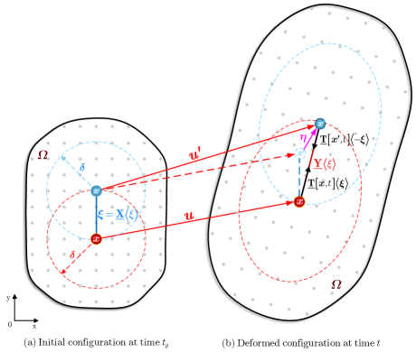
Figure 1: The positions of two material points in the (a) initial and (b) deformed configurations.

As shown in Fig. 1, a domain $\Omega$ modeled by the OSB-PD is composed by material points of infinitesimal volume, where each point would interact with the other points around it within a prescribed horizon radius ($\delta$). Assuming that there is a point $\boldsymbol{x}$ in a domain $\Omega$, and $\boldsymbol{x}^{\prime}$ is a point within its horizon, the hydro-mechanical coupled peridynamic equation of motion at time $t$ can be given as (1):

$$\rho\boldsymbol{\ddot{u}}\left(\boldsymbol{x},t\right)=\int\nolimits_{\mathcal{H}_{x}}\left\{\text{{\@text@baccent{T}}}\left[\boldsymbol{x},p,t\right]\left\langle\boldsymbol{\xi}\right\rangle-\text{ {\@text@baccent{T}}}\left[\boldsymbol{x}^{\prime},p^{\prime},t\right]\left\langle\boldsymbol{-\xi}\right\rangle\right\}dV_{x^{\prime}}+\boldsymbol{b}\left(\boldsymbol{x},t\right)$$ (1)

where $\rho$ is the material mass density, $\boldsymbol{\ddot{u}}$ is the acceleration, $\text{{\@text@baccent{T}}}\left[\boldsymbol{x},p,t\right]\left\langle\boldsymbol{\xi}\right\rangle$ and $\text{ {\@text@baccent{T}}}\left[\boldsymbol{x}^{\prime},p^{\prime},t\right]\left\langle\boldsymbol{-\xi}\right\rangle$ are force density vector states along the deformed bond at points $\boldsymbol{x}$ and $\boldsymbol{x}^{\prime}$, respectively. $dV_{x^{\prime}}$ is the infinitesimal volume associated to point $\boldsymbol{x}^{\prime}$, $\boldsymbol{b}$ is the force density applied by some external force. To describe the position of $\boldsymbol{x}^{\prime}$ with respect to $\boldsymbol{x}$, a relative position vector is defined as:

$$\boldsymbol{\xi=x}^{\prime}-\boldsymbol{x}$$ (2)

After being displaced respectively by $\boldsymbol{u}$ and $\boldsymbol{u}^{\prime}$, the relative displacement vector of $\boldsymbol{x}$ and $\boldsymbol{x}^{\prime}$ is given as:

$$\boldsymbol{\eta}=\boldsymbol{u}^{\prime}-\boldsymbol{u}$$ (3)

To specifically describe the initial and deformed states of the bond in the OSB-PD theory, the reference position vector state, $\underline{\boldsymbol{X}}\left\langle\boldsymbol{\xi}\right\rangle=\boldsymbol{\xi}$, and the deformation vector state, $\underline{\boldsymbol{Y}}\left\langle\boldsymbol{\xi}\right\rangle=\boldsymbol{\xi+\eta}$, are defined. Therefore, the reference position scalar state and the deformation scalar state, representing the lengths of the bond in its initial and deformed state, respectively, are given as:

$$\begin{array}[]{ccc}\underline{x}=\left\|\underline{\boldsymbol{X}}\right\|&,&\underline{y}=\left\|\underline{\boldsymbol{Y}}\right\|\end{array}$$ (4)

where $\left\|\cdot\right\|$ denotes the Euclidean norm.

In a linear OSB-PD material, the elastic strain energy density at point $\boldsymbol{x}$ is given as (49, 39):

$$W\left(\theta,\underline{e}^{d}\right)=\frac{k^{\prime}\theta^{2}}{2}+\frac{\gamma}{2}\int\nolimits_{\mathcal{H}_{x}}\underline{\mathit{w}}\text{ }\underline{e}^{d}\text{ }\underline{e}^{d}\text{d}V_{x^{\prime}}$$ (5)

where $\theta$ is the volume dilatation value, $\underline{e}^{d}$ is the deviatoric extension state, $k^{\prime}$ and $\gamma$ are positive constants related to mechanical material parameters, $\underline{\mathit{w}}$ is an influence function and several examples of its forms have been summarized in (50).

For simplification, only plane strain condition is considered in this paper. $\theta$ and $\underline{e}^{d}$ are usually given as (50):

$$\theta=\frac{2}{m}\int\nolimits_{\mathcal{H}_{x}}\left(\underline{\mathit{w}}\text{ }\underline{x}\text{ }\underline{e}\right)\text{d}V_{x^{\prime}}$$ (6)

$$\underline{e}^{d}=\underline{e}-\frac{\theta\underline{x}}{3}$$ (7)

in which, $\underline{e}$ is the extension scalar state defined as:

$$\underline{e}=\underline{y}-\underline{x}$$ (8)

In plane strain cases, $k^{\prime}$ and $\gamma$ are given as:

$$k^{\prime}=\kappa+\frac{\mu}{9}$$ (9)

$$\gamma=\frac{8\mu}{m}$$ (10)

where $\kappa$ and $\mu$ are bulk modulus and shear modulus, respectively. $m$ is the weighted volume defined as:

$$m=\int\nolimits_{\mathcal{H}_{x}}\underline{\mathit{w}}\left\|\boldsymbol{\xi}\right\|^{2}\text{d}V_{x^{\prime}}$$ (11)

In order to consider the effect of pore pressure on solid deformation, the effective stress principle (51) need to be introduced in the peridynamic model. In (52, 53), an effective force state is proposed in the framework of non-ordinary state-based peridynamics (NOSB-PD) to model geomaterials. The NOSB-PD model is indeed a good choice to simulate the complex behavior of solid materials by introducing the developed classical continuous constitutive relations. In this paper, the ordinary state-based peridynamic model is adopted, and according to (54, 1), the effective force density vector state $\text{{\@text@baccent{T}}}\left[\boldsymbol{x},p,t\right]\left\langle\boldsymbol{\xi}\right\rangle$ in Eq.(1) is defined as:

$$\text{{\@text@baccent{T}}}\left[\boldsymbol{x},p,t\right]\left\langle\boldsymbol{\xi}\right\rangle=\underline{t}\left[\boldsymbol{x},p,t\right]\left\langle\boldsymbol{\xi}\right\rangle\cdot\underline{\boldsymbol{M}}\left\langle\boldsymbol{\xi}\right\rangle$$ (12)

where $\underline{t}$ is called the force density scalar state. $\underline{\boldsymbol{M}}$ is a unit state in the direction of the deformed bond, which is usually defined as:

$$\underline{\boldsymbol{M}}\left\langle\boldsymbol{\xi}\right\rangle=\frac{\underline{\boldsymbol{Y}}}{\left\|\underline{\boldsymbol{Y}}\right\|}$$ (13)

Referring to (54, 1), $\underline{t}\left[\boldsymbol{x},p,t\right]$ is defined in plane strain cases as:

$$\underline{t}\left[\boldsymbol{x},p,t\right]=\left[\left(2k^{\prime}-\frac{1}{9}\gamma m\right)\theta-2\alpha p\right]\frac{\underline{\mathit{w}}\text{ }\underline{x}}{m}+\gamma\underline{\mathit{w}}\text{ }\underline{e}^{d}=\underline{t}\left[\boldsymbol{x},t\right]-2\alpha p\frac{\underline{\mathit{w}}\text{ }\underline{x}}{m}$$ (14)

Thus, the hydro-mechanical coupled peridynamic equation of motion will become:

$$\begin{array}[]{l}\rho\boldsymbol{\ddot{u}}\left(\boldsymbol{x},t\right)=\int\nolimits_{\mathcal{H}_{x}}\left\{\text{{\@text@baccent{T}}}\left[\boldsymbol{x},p,t\right]\left\langle\boldsymbol{\xi}\right\rangle-\text{ {\@text@baccent{T}}}\left[\boldsymbol{x}^{\prime},p^{\prime},t\right]\left\langle\boldsymbol{-\xi}\right\rangle\right\}dV_{x^{\prime}}+\boldsymbol{b}\left(\boldsymbol{x},t\right)\\ =\int\nolimits_{\mathcal{H}_{x}}\left\{\text{{\@text@baccent{T}}}\left[\boldsymbol{x},t\right]\left\langle\boldsymbol{\xi}\right\rangle-\text{ {\@text@baccent{T}}}\left[\boldsymbol{x}^{\prime},t\right]\left\langle\boldsymbol{-\xi}\right\rangle\right\}dV_{x^{\prime}}-2\alpha\int\nolimits_{\mathcal{H}_{x}}\left[p\frac{\underline{\mathit{w}}\text{ }\underline{x}}{m\left(\boldsymbol{x}\right)}\underline{\boldsymbol{M}}\left\langle\boldsymbol{\xi}\right\rangle-\text{ }p^{\prime}\frac{\underline{\mathit{w}}\text{ }\underline{x}}{m\left(\boldsymbol{x}^{\prime}\right)}\underline{\boldsymbol{M}}\left\langle-\boldsymbol{\xi}\right\rangle\right]dV_{x^{\prime}}+\boldsymbol{b}\left(\boldsymbol{x},t\right)\end{array}$$ (15)

where $p$ and $p^{\prime}$ are the values of pore pressure at points $\boldsymbol{x}$ and $\boldsymbol{x}^{\prime}$.

2.2 Failure criteria

Failure criteria are essential in PD-based numerical models to describe material failure and crack advancement. In (55), a strain energy-based “critical bond stretch” failure criterion is introduced for state-based PD model and successfully applied to the quantitative fracture analysis of solid materials. Here we adopt that failure criterion for convenience.

As in (55), when the stretch value of a bond reaches the critical value $s_{c}$, it will be broken, indicating the advancement of fracture. The stretch value of bond $\boldsymbol{\xi}$ is defined as (50):

$$s\left\langle\boldsymbol{\xi}\right\rangle=\frac{\underline{e}\left\langle\boldsymbol{\xi}\right\rangle}{\underline{x}\left\langle\boldsymbol{\xi}\right\rangle}$$ (16)

thus, the extension scalar state can be also expressed as:

$$\underline{e}\left\langle\boldsymbol{\xi}\right\rangle=s\left\langle\boldsymbol{\xi}\right\rangle\text{ }\underline{x}\left\langle\boldsymbol{\xi}\right\rangle$$ (17)

As shown in Fig. 2, $\mathcal{H}_{l}$ is the domain removed by the crack surface from the neighborhood of point $\boldsymbol{x}$. $\boldsymbol{x}^{\prime}$ represents points located in the domain $\mathcal{H}_{l}$. The bond connecting $\boldsymbol{x}$ and $\boldsymbol{x}^{\prime}$ is marked as $\boldsymbol{\xi}$. At the formation of the crack surface, the deformation energy stored in the bond $\boldsymbol{\xi}$ is released. Therefore, we could assume that the work required to break all the bonds connecting point $\boldsymbol{x}$ to points in the domain $\mathcal{H}_{l}$ is equal to the summation of the energy stored in these bonds in their critical stretch condition. In critical condition, the extension scalar states of these bonds are $\underline{e}_{c}=s_{c}$ $\underline{x}$.

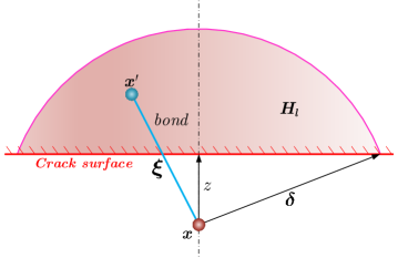
Figure 2: A diagrammatic sketch of a peridynamic domain crossed by a crack surface.

According to the definition of $\theta$ in Eq. (6), the volume dilatation value caused by the broken bonds can be computed by:

$$\theta_{\boldsymbol{l}}=\frac{2}{m}\int\nolimits_{\mathcal{H}_{l}}\left(\underline{\mathit{w}}\text{ }\underline{x}\text{ }\underline{e}_{c}\right)\text{ d}V_{x^{\prime}}=\frac{2}{m}\int\nolimits_{\mathcal{H}_{l}}\left(\underline{\mathit{w}}\text{ }\underline{x}^{2}\text{ }s_{c}\right)\text{ d}V_{x^{\prime}}=2\varpi_{l}\text{ }s_{c}$$ (18)

where

$$\begin{array}[]{ccc}\varpi_{l}=\frac{m_{l}}{m}&\&&m_{l}=\int\nolimits_{\mathcal{H}_{l}}\left(\underline{\mathit{w}}\text{ }\underline{x}^{2}\right)dV_{x^{\prime}}\end{array}$$ (19)

is the volume weight from the points in the domain $\mathcal{H}_{l}$, and $\varpi_{l}=\frac{m_{l}}{m}$ is the ratio of $m_{l}$ to $m$.

Using Eqs. (5), (6), (9) and (10), the expression of strain energy density can be rewritten as (55, 49):

$$W\left(\theta,\underline{e}\right)=\frac{1}{2}\left(\kappa-\frac{7}{9}\mu\right)\theta^{2}+\frac{4\mu}{m}\int\nolimits_{\mathcal{H}_{x}}\underline{\mathit{w}}\text{ }\underline{e}\text{ }\underline{e}\text{ }\text{d}V_{x^{\prime}}$$ (20)

Accordingly, substitution of Eqs. (18-19) into (20) gives the energy released by the broken bonds at point $\boldsymbol{x}$ as:

$$W\left\langle\boldsymbol{x}\right\rangle=\frac{1}{2}\left(\kappa-\frac{7}{9}\mu\right)\theta_{\boldsymbol{l}}^{2}+\frac{4\mu}{m}\int\nolimits_{\mathcal{H}_{l}}\underline{\mathit{w}}\text{ }\underline{x}^{2}\text{ }s_{c}^{2}\text{d}V_{x^{\prime}}=\left[2\varpi_{l}^{2}\left(\kappa-\frac{7}{9}\mu\right)+4\mu\varpi_{l}\right]s_{c}^{2}\text{ }$$ (21)

Consequently, the released energy per unit fracture area is:

$$G_{c}=2\int\nolimits_{0}^{\delta}W\left\langle\boldsymbol{x}\right\rangle\text{ d}z=2\int\nolimits_{0}^{\delta}\left[2\varpi_{l}^{2}\left(\kappa-\frac{7}{9}\mu\right)+4\mu\varpi_{l}\right]s_{c}^{2}\text{ d}z=\left[4\left(\kappa-\frac{7}{9}\mu\right)\beta+8\mu\beta^{\prime}\right]s_{c}^{2}$$ (22)

In Eq. (22), $\beta$ and $\beta^{\prime}$ are parameters affected by the influence function, and are defined as:

$$\begin{array}[]{ccc}\beta=\int\nolimits_{0}^{\delta}\varpi_{l}^{2}\text{ d}z&,&\beta^{\prime}=\int\nolimits_{0}^{\delta}\varpi_{l}\text{ d}z\end{array}$$ (23)

In this paper, the influence function is taken as $\underline{\mathit{w}}=1$, therefore, the values of $\beta$ and $\beta^{\prime}$ can be obtained as:

$$\begin{array}[]{ccc}\beta=0.2192\delta&,&\beta^{\prime}=\frac{2\delta}{5\pi}\end{array}$$ (24)

According to Eq. (22), the critical stretch value $s_{c}$ of plane strain OSB-PD model can be given as:

$$s_{c}=\sqrt{\frac{G_{c}}{\left[4\left(\kappa-\frac{7}{9}\mu\right)\beta+8\mu\beta^{\prime}\right]}}$$ (25)

where $G_{c}$ is the critical energy release rate for mode I fracture. The effect of damage can be taken into account by introducing a variable $\mathit{\varrho}$, in a way similar to that used in BB-PD models (44, 56):

$$\underline{\mathit{\varrho}}\left\langle\boldsymbol{\xi}\right\rangle\boldsymbol{=}\left\{\begin{array}[]{ccc}1&,&\text{if }s\left\langle\boldsymbol{\xi}\right\rangle<s_{c}\text{ , for all }0<\overline{t}<t\\ 0&,&\text{otherwise}\end{array}\right.$$ (26)

then the damage value $\varphi_{x}$ at point $\boldsymbol{x}$ in the system can be defined as:

$$\varphi_{x}=1-\frac{\int\nolimits_{\mathcal{H}_{x}}\underline{\mathit{w}}\left\langle\boldsymbol{\xi}\right\rangle\text{ }\underline{\mathit{\ \varrho}}\left\langle\boldsymbol{\xi}\right\rangle\text{d}V_{x^{\prime}}}{\int\nolimits_{\mathcal{H}_{x}}\underline{\mathit{w}}\left\langle\boldsymbol{\xi}\right\rangle\text{d}V_{x^{\prime}}}$$ (27)

where $\varphi_{x}\in\left[0,1\right]$, and the cracks can be identified wherever $\varphi_{x}\geqslant 0.5$.

2.3 Formulation for fluid flow in fractured porous media

In this paper, we use Darcy’s law to describe the flow field in the saturated porous domain $\Omega$. Other more complicated flow field models will be considered in future work. To formulate the governing equation for flow in the fractured porous domain, the whole domain $\Omega$ is divided into three parts: $\Omega_{r}$, $\Omega_{f}$ and $\Omega_{t}$ (see Fig. 3a), representing the unbroken domain (reservoir domain), the fracture domain and the transition domain between $\Omega_{r}$ and $\Omega_{f}$. The peridynamic damage field ($\varphi$ in Eq. (27)) is used as an indicator. As shown in Fig. 3b, two threshold values ($c_{1}$ and $c_{2}$) are set to identify the three flow domains: the reservoir domain is defined as $\varphi\leqslant c_{1}$, the fracture domain as $\varphi\geqslant c_{2}$ and the transition domain as $c_{1}\leq\varphi\leq c_{2}$.

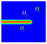
(a)

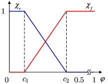
(b)

Figure 3: (a) The definition of the $\Omega_{r}$, $\Omega_{t}$ and $\Omega_{f}$; (b) linear indicator functions $\chi_{r}$ and $\chi_{f}$.

Therefore, the mass balance equation for the reservoir domain is given as:

$$\rho_{r}s_{r}\frac{\partial p}{\partial t}+\rho_{r}\alpha_{r}\frac{\partial\varepsilon_{v}}{\partial t}+\rho_{r}\nabla\cdot\left[\frac{k_{r}}{\mu_{w}}\left(-\nabla p+\rho_{r}g\right)\right]=q_{r}$$ (28)

where $\alpha_{r}$, $s_{r}$, $k_{r}$, $q_{r}$ and $\rho_{r}$ are the Biot coefficient, storage coefficient, permeability, source term and the density of the medium in the reservoir domain, respectively; $\mu_{w}$ is the viscosity coefficient of the fluid in the reservoir domain. $g$ is gravity and $\varepsilon_{v}$ is volumetric strain. The storage coefficient is given as:

$$s_{r}=\frac{\left(\alpha_{r}-n_{r}\right)\left(1-\alpha_{r}\right)}{K_{r}}+\frac{n_{r}}{K_{w}}$$ (29)

where $K_{r}$ and $K_{w}$ are the bulk moduli of solid and fluid in the reservoir domain, $n_{r}$ is the porosity.

The fracture domain is assumed to be fully filled by fluid and the porosity $n_{f}=1$ is adopted. Supposing that the fluid in the fracture is incompressible, the volumetric strain term in Eq. (28) vanishes (57, 58), and the mass balance in the fracture domain is expressed as:

$$\rho_{f}s_{f}\frac{\partial p}{\partial t}+\rho_{f}\nabla\cdot\left[\frac{k_{f}}{\mu_{w}}\left(-\nabla p+\rho_{f}g\right)\right]=q_{f}$$ (30)

where $s_{f}$, $k_{f}$, $q_{f}$ and $\rho_{f}$ are the storage coefficient, permeability, source term and the density of the fluid in the fracture domain.

Two linear indicator functions are defined to connect the transition domain with the reservoir and fracture domains: $\chi_{r}$ and $\chi_{f}$ (58, 59, 60), and they satisfy:

$$\chi_{r}\left(\cdot,\varphi\right):=\chi_{r}\left(\boldsymbol{x},t,\varphi\right)=1\text{ in }\Omega_{r}\left(t\right)\text{ and }\chi_{r}\left(\cdot,\varphi\right)=0\text{ in }\Omega_{f}\left(t\right)$$ (31)

$$\chi_{f}\left(\cdot,\varphi\right):=\chi_{f}\left(\boldsymbol{x},t,\varphi\right)=1\text{ in }\Omega_{f}\left(t\right)\text{ and }\chi_{f}\left(\cdot,\varphi\right)=0\text{ in }\Omega_{r}\left(t\right)$$ (32)

As described in Fig. 3b, the two linear functions are defined as:

$$\chi_{r}\left(\cdot,\varphi\right)=\frac{c_{2}-\varphi}{c_{2}-c_{1}},\text{ and }\chi_{f}\left(\cdot,\varphi\right)=\frac{\varphi-c_{1}}{c_{2}-c_{1}}$$ (33)

Fluid and solid properties in the transition domain can be obtained by interpolating those properties of reservoir and fracture domains by using the indicator functions: $\rho_{T}=\rho_{r}\chi_{r}+\rho_{f}\chi_{f}$, $\alpha_{T}=\alpha_{r}\chi_{r}+\alpha_{f}\chi_{f}$, $n_{T}=n_{r}\chi_{r}+n_{f}\chi_{f}$, $k_{T}=k_{r}\chi_{r}+k_{f}\chi_{f}$, $s_{T}=s_{r}\chi_{r}+s_{f}\chi_{f}$. It should be noted in particular that the Biot coefficient in the fracture domain is taken as $\alpha_{f}=1$. Therefore, the governing equation for the fluid flow in the transition domain can be given as:

$$\rho_{T}s_{T}\frac{\partial p}{\partial t}+\rho_{T}\alpha_{T}\frac{\partial\varepsilon_{v}}{\partial t}+\rho_{T}\nabla\cdot\left[\frac{k_{T}}{\mu_{w}}\left(-\nabla p+\rho_{T}g\right)\right]=q_{T}$$ (34)

Moreover, the cubic law is used to evaluate the permeability in the fracture domain (61, 29):

$$k_{f}=\frac{1}{12}a^{2}$$ (35)

where $a$ is the aperture of the crack, and it can be obtained by using the method described in the $sect.$ $3.3$ of (1).

3 Discretization and numerical solution procedure

Following the description of the hybrid modeling approach in (1), the Galerkin finite element method is adopted for the governing equation of the fluid flow, while the peridynamics for the deformation of the solid phase. The fluid domain is discretized by using 4-node FE elements and the solid domain by using a regular PD grid. PD and FE nodes share the same coordinates, but this is not required by our approach. The implementation of the hydro-mechanical coupling process is described in Fig. 4.

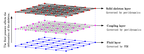
(a) Effect of fluid on solid.

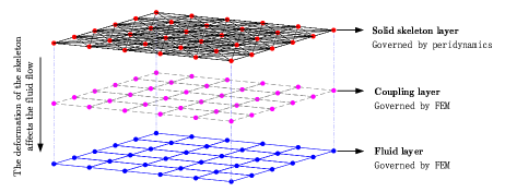
(b) Effect of solid on fluid.

Figure 4: Schematic diagram of bidirectional influence in the coupling process, redrawn with permission from Ni et al. (1).

3.1 Discretization of governing equations

The discretized peridynamic equation of motion of the current node $\boldsymbol{x}_{i}$ is written as:

$$\begin{array}[]{l}\rho\boldsymbol{\ddot{u}}_{i}^{t}=\sum_{j=1}^{N_{H_{i}}}\left\{\text{ {\@text@baccent{T}}}\left[\boldsymbol{x}_{i},t\right]\left\langle\boldsymbol{\xi}_{ij}\right\rangle-\text{ {\@text@baccent{T}}}\left[\boldsymbol{x}_{j},t\right]\left\langle\boldsymbol{-\xi}_{ij}\right\rangle\right\}\cdot V_{j}\\ -2\alpha\sum_{j=1}^{N_{H_{i}}}\left[p_{i}\frac{\underline{\mathit{w}}\left\langle\boldsymbol{\xi}_{ij}\right\rangle\text{ }\underline{x}\left\langle\boldsymbol{\xi}_{ij}\right\rangle}{m\left(\boldsymbol{x}_{i}\right)}\underline{\boldsymbol{M}}\left\langle\boldsymbol{\xi}_{ij}\right\rangle-\text{ }p_{j}\frac{\underline{\mathit{w}}\left\langle\boldsymbol{\xi}_{ij}\right\rangle\text{ }\underline{x}\left\langle\boldsymbol{\xi}_{ij}\right\rangle}{m\left(\boldsymbol{x}_{j}\right)}\underline{\boldsymbol{M}}\left\langle-\boldsymbol{\xi}_{ij}\right\rangle\right]\cdot V_{j}+\boldsymbol{b}_{i}^{t}\end{array}$$ (36)

where $N_{H_{i}}$ is the number of family nodes of $\boldsymbol{x}_{i}$, $\boldsymbol{x}_{j}$ represents $\boldsymbol{x}_{i}$’s family node, $V_{j}$ is the volume of node $\boldsymbol{x}_{j}$.

Under the assumption of small deformation, the global form of Eq.(36) can be written as:

$$\boldsymbol{M}^{PD}\boldsymbol{\ddot{u}}+\boldsymbol{K}^{PD}\boldsymbol{u}-\boldsymbol{Q}^{PD}p=f^{PD}$$ (37)

in which $\boldsymbol{M}^{PD}$, $\boldsymbol{K}^{PD}$ and $\boldsymbol{Q}^{PD}$ are the mass, stiffness and “coupling” matrices of the PD domain, respectively. Note that $\boldsymbol{M}^{PD}$ is usually taken as a lumped mass matrix. The method of obtaining $\boldsymbol{K}^{PD}$ of OSB-PD equations can be found in (62). Assuming that $\underline{\boldsymbol{M}}\left\langle\boldsymbol{\xi}_{ij}\right\rangle=\left[M_{x},M_{y}\right]$, then the “coupling” matrix for $\boldsymbol{\xi}_{ij}$ can be given as:

$$\boldsymbol{Q_{ij}^{PD}=}2\alpha\underline{\mathit{w}}\left\langle\boldsymbol{\xi}_{ij}\right\rangle\underline{x}\left\langle\boldsymbol{\ \xi}_{ij}\right\rangle V_{i}V_{j}\left[\begin{array}[]{cccc}\frac{M_{x}}{m\left(\boldsymbol{x}_{i}\right)}&\frac{M_{y}}{m\left(\boldsymbol{x}_{i}\right)}&-\frac{M_{x}}{m\left(\boldsymbol{x}_{i}\right)}&-\frac{M_{y}}{m\left(\boldsymbol{x}_{i}\right)}\\ \frac{M_{x}}{m\left(\boldsymbol{x}_{j}\right)}&\frac{M_{y}}{m\left(\boldsymbol{x}_{j}\right)}&-\frac{M_{x}}{m\left(\boldsymbol{x}_{j}\right)}&-\frac{M_{y}}{m\left(\boldsymbol{x}_{j}\right)}\end{array}\right]^{T}$$ (38)

where the influence function $\underline{\mathit{w}}\left\langle\boldsymbol{\ \xi}_{ij}\right\rangle$ used for the coupling bonds should be specified as $\underline{\mathit{w}}=1$.

The discretized governing equations of the fluid flow assume the following form (51):

$$\boldsymbol{S\dot{p}}+\boldsymbol{Q}^{T}\boldsymbol{\dot{u}}+\boldsymbol{Hp=q}^{w}$$ (39)

where $\boldsymbol{Q}$ is the coupling matrix, $\boldsymbol{H}$ is the permeability matrix, $\boldsymbol{S}$ is the compressibility matrix, all of them can be obtained by assembling the corresponding element matrices. When using the shape functions $\boldsymbol{N}_{u}$ (for displacement) and $\boldsymbol{N}_{p}$ (for pressure), the matrices in Eq.(39) can be given as (46, 3):

$$\boldsymbol{Q=}\int\nolimits_{\Omega}\left(\boldsymbol{LN}_{u}\right)^{T}\alpha\boldsymbol{mN}_{p}\text{d}\Omega$$ (40)

$$\boldsymbol{H=}\int\nolimits_{\Omega}\left(\nabla\boldsymbol{N}_{p}\right)^{T}\frac{k}{\mu_{w}}\left(\nabla\boldsymbol{N}_{p}\right)\text{d}\Omega$$ (41)

$$\boldsymbol{S=}\int\nolimits_{\Omega}\boldsymbol{N}_{p}^{T}s\boldsymbol{N}_{p}\text{d}\Omega$$ (42)

in which $\boldsymbol{L}$ is the differential operator defined as:

$$\boldsymbol{L=}\left[\begin{array}[]{ccc}\frac{\partial}{\partial x}&0&\frac{\partial}{\partial y}\\ 0&\frac{\partial}{\partial y}&\frac{\partial}{\partial x}\end{array}\right]^{T}$$ (43)

$\boldsymbol{m}$ is a vector given as:

$$\boldsymbol{m}=\left[1,1,0\right]^{T}$$ (44)

As described in $sect.$ $3.3$, the volumetric coupling term $\left(\rho\alpha\frac{\partial\varepsilon_{v}}{\partial t}\right)$ will be removed from the governing equation for the flow in the fracture domain.

3.2 Staggered solution scheme of the hydro-mechanical coupled system

As in (51, 47), Eqs. 37 and 39 can be combined and rewritten in the following format:

$$\left[\begin{array}[]{cc}\boldsymbol{M}^{PD}&\boldsymbol{0}\\ \boldsymbol{0}&\boldsymbol{0}\end{array}\right]\left[\begin{array}[]{c}\boldsymbol{\ddot{u}}\\ \boldsymbol{\ddot{p}}\end{array}\right]+\left[\begin{array}[]{cc}\boldsymbol{0}&\boldsymbol{0}\\ \boldsymbol{Q}^{T}&\boldsymbol{S}\end{array}\right]\left[\begin{array}[]{c}\boldsymbol{\dot{u}}\\ \boldsymbol{\dot{p}}\end{array}\right]+\left[\begin{array}[]{cc}\boldsymbol{K}^{PD}&\boldsymbol{-Q}^{PD}\\ \boldsymbol{0}&\boldsymbol{H}\end{array}\right]\left[\begin{array}[]{c}\boldsymbol{u}\\ \boldsymbol{p}\end{array}\right]=\left[\begin{array}[]{c}\boldsymbol{f}\\ \boldsymbol{q}^{w}\end{array}\right]$$ (45)

“Monolithic” and “staggered” algorithms are commonly adopted to solve such a coupled system. Details of the “monolithic” solution algorithm can be found in (47, 3, 1). It is usually both memory- and time-intensive when used for the solution of hydro-mechanical coupled problems involving fracture advancement. Therefore often, a “staggered” algorithm is preferred to obtain the dynamic solutions of such kind of coupled problems.

In a “staggered” algorithm, the first row and second row in Eq. 45 are solved sequentially, and the previously solved field variables ($\boldsymbol{u}$ and $\boldsymbol{p}$) are used as conditions of the next solving sequence. For the described hydro-mechanical coupled problems, the two steps in each solving sequence can be summarized as follows:

–step 1: solve the pressure field ($\boldsymbol{p}^{n+1}$) using the following implicit time integration iteration (1):

$$\boldsymbol{p}^{n+1}=\left[\boldsymbol{S}+\vartheta\Delta t\boldsymbol{H}\right]^{-1}\left\{\left[\boldsymbol{S}-\left(1-\vartheta\right)\Delta t\boldsymbol{H}\right]\boldsymbol{p}^{n}-\Delta t\boldsymbol{q}^{w}+\boldsymbol{Q}^{T}\left(\mathbf{u}^{n}-\mathbf{u}^{n-1}\right)\right\}$$ (46)

–step 2: solve the displacement field ($\boldsymbol{u}^{n+1}$) of the solid domain by using appropriate time integration algorithm.

This paper aims to capture the dynamic phenomena in hydraulic fracture problems. Thus, a modified explicit central difference time integration scheme proposed in (48) is adopted here to obtain the dynamic solution of the OSB-PD model. In the chosen time integration scheme, the velocities are integrated with a forward difference and the displacements with a backward difference. The velocity and displacement at the $\left(n+1\right)^{th}$ time increment can be obtained as:

$$\begin{array}[]{l}\boldsymbol{\dot{u}}^{n+1}=\boldsymbol{\dot{u}}^{n}+\Delta t\boldsymbol{\ddot{u}}^{n}\\ \boldsymbol{u}^{n+1}=\boldsymbol{u}^{n}+\Delta t\boldsymbol{\dot{u}}^{n+1}\end{array}$$ (47)

where $\boldsymbol{\ddot{u}}^{n}$ is the acceleration at $n^{th}$ time increment and can be determined by using Newton’s second law:

$$\boldsymbol{\ddot{u}}^{n+1}=\mathbf{M}^{-1}\left(\mathbf{F}^{ext}-\mathbf{F}^{int}-\boldsymbol{Q}^{PD}\boldsymbol{p}\right)$$ (48)

where $\mathbf{F}^{ext}$ and $\mathbf{F}^{int}$ are the external and internal force vectors, respectively, $\mathbf{M}$ is the diagonal mass matrix. The $\Delta t$ in the above equations is the constant time increment, and the explicit method for the undamped system requires a critical time step for numerical stability. According to (63), the stable time increment for PD model can be defined as:

$$\Delta t<\delta/c^{\prime}$$ (49)

where $c^{\prime}=\sqrt{\left(\lambda+2\mu\right)/\rho}$ is the dilatational wave speed and $\lambda$ and $\mu$ are the Lame’s elastic constants of the material.

Note that the permeability and storage matrices ($\boldsymbol{H}$ and $\boldsymbol{S}$) need to be updated accordingly in each time step when involving cracks.

Remark 1. The FE formulation for fluid flow, even if local, contains de facto a length scale due to the fact that we have the natural presence of a gradient term through Darcy’s Law and this inside a divergence operator. The result is a Laplace’s operator which is known to introduce a length scale even if sometimes weak. This fact has been extensively investigated in dynamic strain localization analysis (64). As stated in (1), when solving the hybrid model, the coupling matrices in the first row and second row of Eq. (45) should be generated non-locally and locally, respectively. However, because of the inconsistency of the length scales in the hybrid local and non-local coupled system, it has been found that it may entail problems in the simulation of dynamic problems. It is usually difficult to ensure the consistency of length scales in the both domains. Thus, although not theoretically rigorous, it is a convenient choice to adopt the same formulation of coupling matrices to avoid numerical instability. In addition, recently some criticism has been put forward about wave dispersion characteristics of PD models in (65), which could be another factor affecting the dynamic solutions of the coupled system and deserves further scrutiny.

4 Wave propagation in one-dimensional dynamic consolidation problem: a benchmark case

In this section, an example of one-dimensional dynamic consolidation is presented to validate the proposed approach. This example was solved by Schanz and Cheng (66) for the transient wave propagation of the displacement and pore pressure during the dynamic consolidation process and analytical solutions were obtained by using the Dubner and Abate’s method (67) for comparison. In order to reproduce this example and compare our solution with the analytical one, the behavior of a poroelastic column shown in Fig. 5 is simulated under the following boundary conditions. The top is drained with a pore pressure of $p=0$ and subjected to a sudden surface pressure $P_{s}=1Pa$, while the other boundaries are impermeable and constrained in their normal direction. The mechanical and fluid parameters used in the simulations are listed in Tab. 1. Referring to (66), a fixed time step of $\Delta t=1\times 10^{-5}s$ and $\vartheta=0.5$ are chosen for the time integration.

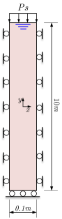
Figure 5: Geometry and boundary conditions of the one-dimensional dynamic consolidation problem.

Table 1: Mechanical and fluid parameters used in the example of dynamic consolidation problem.

$E$	$\nu$	$\rho_{r}$	$\rho_{w}$	$\alpha$
$0.254GPa$	$0.3$	$2700kg/m^{3}$	$1000kg/m^{3}$	$0.7883$
$n$	$K_{r}$	$K_{w}$	$\mu$	$k$
$0.48$	$11GPa$	$3.3GPa$	$1\times 10^{-3}Pa\cdot s$	$3.55\times 10^{-12}m^{2}$

Discretization parameters are the key factors affecting the solutions of peridynamic models (68). It is therefore necessary to perform convergence studies on discretization parameters before using peridynamic-based tools for numerical analysis. $\delta$-convergence and $m_{r}$-convergence studies are hence performed here to identify the most suitable discretization parameters in terms of accuracy and computational cost. In the $m_{r}$-convergence study, the $\delta=0.015m$ and $m_{r}=2,3,4,5$ are adopted respectively. The variations of the vertical displacement on top edge and pore pressure on the bottom edge are plotted in Figs. 6a and 6b, respectively. The comparison between the numerical and analytical solutions suggests that $m_{r}=2$ is an acceptable choice for such a hydro-mechanical coupled problem if both the accuracy of displacement and pore pressure are considered. Consequently, $m_{r}=2$ in conjunction with $\delta=0.012m,0.015m,0.018m,0.02m$ are chosen for the $\delta$-convergence study. The numerical solutions of the $\delta$-convergence study are plotted in Figs. 7a and 7b. According to the numerical results, we can conclude that the proposed hybrid modeling approach can properly simulate the dynamic response in saturated porous media. However, the discretization parameters of peridynamic models have a remarkable influence on simulation results. The proposed PD-based hybrid model shows a different convergence performance in such a hydro-mechanical coupled problem from that in mechanical-only problems (68). In general, $m_{r}=2$ is an economical choice to obtain acceptable results with the hybrid model when choosing the appropriate grid size.

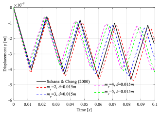
(a) Variation of vertical displacement on the top edge versus time.

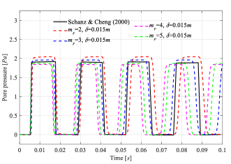
(b) Variation of pore pressure on the bottom edge versus time.

Figure 6: $m_{r}$-convergence study of the dynamic consolidation example with $\delta=0.015m$.

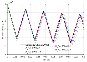
(a) Variation of vertical displacement on the top edge versus time.

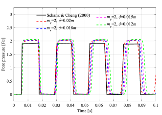
(b) Variation of pore pressure on the bottom edge versus time.

Figure 7: $\delta$-convergence study of the dynamic consolidation example with $m_{r}=2$.

5 Dynamic forerunning fracture in porous structures

In (2, 3, 4), a cantilever beam sample was adopted to study the stepwise crack advancement and fluid pressure oscillations in porous media fracturing dynamics. In (4) as well as in (31), fracture advancement with forerunning was observed in the dry case. Inspired by that, a rectangular structure is solved in this section by using the proposed approach for investigating dynamic fracturing with possible forerunning in both dry and fully saturated porous media. The geometry and constraints of the selected structure are drawn in Fig. 8a. Two different loading conditions, mechanical loading and fluid injection, are adopted as respectively shown in Fig. 8b. The mechanical and fluid parameters used in the simulations are listed in Tab. 2. Note that the fracture energy release rate is taken as $G_{c}=1J/m^{2}$ for making it easier to achieve fracture advancement in the structure. Since the described problem is symmetric, only the right half of the structure is modeled in the simulation. The whole domain is discretized by quadrilateral meshes with grid size of $\Delta x=2.5\times 10^{-3}m$. $m_{r}=2$ is used for the peridynamic model and thus the horizon radius is $\delta=2\times\Delta x=5\times 10^{-3}m$. A fixed time step of $\Delta t=1\times 10^{-7}s$ and $\vartheta=0.5$ are used for the time integration. The simulation time duration is chosen as $1\times 10^{-3}s$. The boundary conditions of the solid and fluid portions are applied non-locally and locally, respectively. The method of applying boundary conditions to peridynamic model can be found in (56), and to FEM model in (51). According to the two loading conditions and the material saturation, three different cases are solved. For the purpose of guiding the wave propagation, the crack is only allowed to propagate along the horizontal centerline of the specimen.

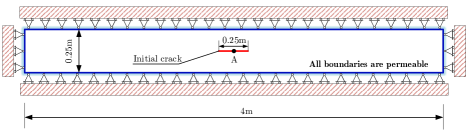
(a) Geometry and constraints.

(b) Loading conditions.

Figure 8: Geometry and boundary conditions of the rectangular structure with a central initial crack.

Table 2: Mechanical and fluid parameters used in the forerunning fracturing examples.

$E$	$\nu$	$G_{c}$	$\rho_{r}$	$\rho_{w}$
$10GPa$	$0.25$	$1J/m^{2}$	$1000kg/m^{3}$	$1000kg/m^{3}$
$\alpha$	$n$	$K_{w}$	$\mu$	$k$
$1$	$0.002$	$2.2GPa$	$1\times 10^{-3}Pa\cdot s$	$1\times 10^{-12}m^{2}$

The first case (case 1) considers a dry porous material under mechanical loading condition. As shown in Fig. 8b, a constant pressure $\boldsymbol{\sigma}=15MPa$ is applied on the surface of the initial crack near the central position to force crack opening. Under the action of the external force, the crack propagates from the initial crack tip. As shown in Figs. 9a to 9d, forerunning events are observed during the simulation.

(a) Damage levels at $2.77\times 10^{-4}s$.

(b) Damage levels at $4.42\times 10^{-4}s$.

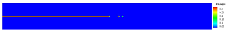
(c) Damage levels at $8\times 10^{-4}s$.

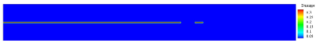
(d) Damage levels at $1\times 10^{-3}s$.

Figure 9: Forerunning fracture in the front of the crack tip in dry structure under mechanical loading condition.

The second case (case 2) is carried out with a saturated porous material under mechanical loading condition by applying the same constant pressure on the surface of the initial crack. Under the action of applied external force, the initial crack opens gradually, the material domain deforms and the pore pressure in the whole domain changes accordingly. In this case, the crack propagation occurs under the combined action of external force and pore pressure. As shown in Figs. 10a to 10d, forerunning events also exist in this case. The distributions of pore pressure at $2.5\times 10^{-4}s$, $2.6\times 10^{-4}s$, $2.7\times 10^{-4}s$ and $2.8\times 10^{-4}s$ are plotted in Figs. 11a to 11d, respectively. Changes shown in these images reveal the wave propagation of pore pressure in the simulated structure. It is worth to observe by comparing the fracture position reached after $1\times 10^{-3}s$ that the fracture propagates faster in the saturated medium thanks to the combined action of stress and pressure waves, and this result can also be inferred from Fig. 14.

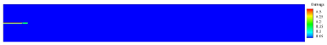
(a) Damage levels at $4\times 10^{-5}s$.

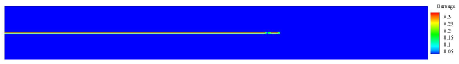
(b) Damage levels at $7.56\times 10^{-4}s$.

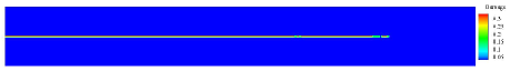
(c) Damage levels at $9.41\times 10^{-4}s$.

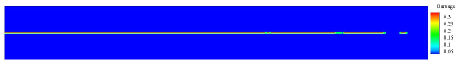
(d) Damage levels at $1\times 10^{-3}s$.

Figure 10: Forerunning fracture in the front of the crack tip in saturated structure under mechanical loading condition.

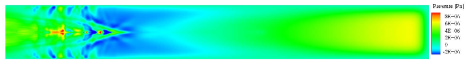
(a) Distribution of pore pressure at $2.5\times 10^{-4}s$.

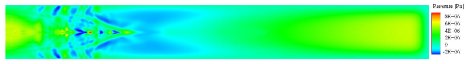
(b) Distribution of pore pressure at $2.6\times 10^{-4}s$.

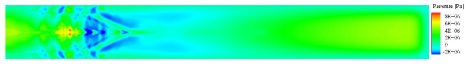
(c) Distribution of pore pressure at $2.7\times 10^{-4}s$.

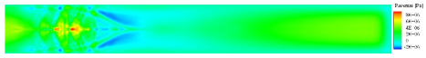
(d) Distribution of pore pressure at $2.8\times 10^{-4}s$.

Figure 11: Wave propagation of pore pressure in saturated structure under mechanical loading condition.

The last case (case 3) is carried out with the saturated porous material under the fluid injection. The fluid is injected at the center of initial crack with a constant volume rate of $Q=1m^{3}/s$. Figs. 12a to 12d show the crack patterns in this case at four different time instants during the fracture process, and cracks are also observed in front of the tip of the continuous crack. The distributions of pore pressure at four time instants ($2.3\times 10^{-4}s$, $2.4\times 10^{-4}s$, $2.5\times 10^{-4}s$ and $2.6\times 10^{-4}s$) are plotted in Figs. 13a to 13d, respectively. A dynamic phenomenon of wave propagation of pore pressure is also observed.

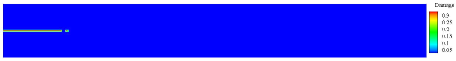
(a) Damage levels at $1.54\times 10^{-4}s$.

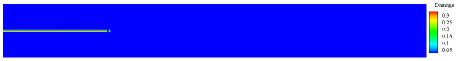
(b) Damage levels at $3.38\times 10^{-4}s$.

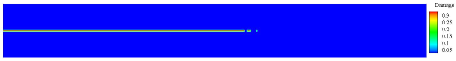
(c) Damage levels at $5.51\times 10^{-4}s$.

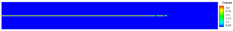
(d) Damage levels at $7.23\times 10^{-4}s$.

Figure 12: Forerunning fracture in the front of the crack tip in saturated structure under fluid injection.

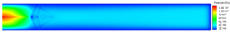
(a) Distribution of pore pressure at $2.3\times 10^{-4}s$.

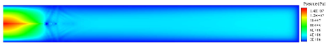
(b) Distribution of pore pressure at $2.4\times 10^{-4}s$.

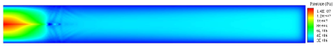
(c) Distribution of pore pressure at $2.5\times 10^{-4}s$.

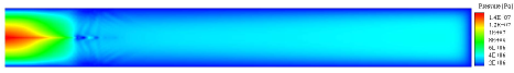
(d) Distribution of pore pressure at $2.6\times 10^{-4}s$.

Figure 13: Wave propagation of pore pressure in saturated structure under fluid injection.

The variation of crack length with time in the three cases is plotted in Fig. 14. The solid dots marked in Fig. 14 correspond to the time instants in Figs. 9, 10 and 12, respectively. Based on the locations of these solid dots and their corresponding distributions of damage levels, it can be found that there appears a jump in crack advancement when forerunning fracture occurs. All the examples shown in this section suggest numerically that the stepwise advancement of fractures and the forerunning fracturing phenomenon stressed in (2, 4) do exist in the dynamic fracture of dry and saturated porous media.

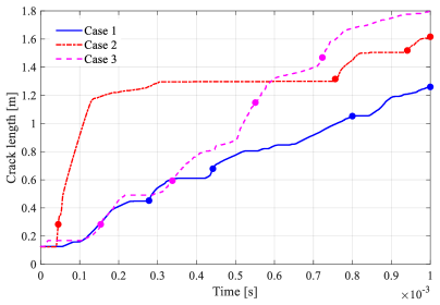
Figure 14: Variation of crack length with time; case 1 is a dry structure under mechanical loading, case 2 a saturated structure under mechanical loading and case 3 a saturated structure with fluid injection.

6 Conclusions

The hybrid FEM and Peridynamic modeling approach proposed in (1) is applied here to solve the problem of dynamic fracture propagation in saturated porous media. In the hybrid modeling approach, the fluid flow is governed by FE equations, while peridynamics is used to solve the deformation of solids and capture the dynamic fracture advancement. A staggered solution scheme is adopted to obtain the dynamic solution of the hydro-mechanical coupled system. In each solving sequence, an implicit time integration iteration from (47) is used to solve the FE equations of fluid flow, and a modified explicit central difference time integration algorithm proposed in (48) is adopted for the peridynamic equations.

Firstly, an example of a one-dimensional dynamic consolidation problem is solved by the presented approach as a benchmark case. Both $\delta-$convergence and $m_{r}-$convergence studies are performed to investigate the influences of discretization parameters on the dynamic solutions of such a coupled problem. Based on the comparison of numerical results and analytical solutions, $m_{r}=2$ is suggested for the PD portion to obtain acceptable dynamic solution of the described hydro-mechanical coupled system. Subsequently, a series of numerical simulations of the dynamic crack propagation in dry and fully saturated porous structures are carried out. Forerunning fracture events, a phenomenon that has been observed experimentally in geomaterials (30), occur in these simulations. Besides the mechanical wave, the wave propagation of pore pressure has also been numerically confirmed to exist in saturated porous structures. The interaction between mechanical waves and pore pressure waves makes dynamic fracturing in saturated media more complicated, influencing also the forerunning episodes. It is worth to point out that in (69) it has been shown that in dry bodies (i) forerunning is a undeniable source of stepwise fracturing advancement; (ii) forerunning is a stability problem; and (iii) forerunning increases the overall tip advancement speed and is, in fact, a mechanism for a crack to move faster when a steady-state propagation is no longer supported by the body due to a high level of external forces. It appears clearly from Fig. 14 that the interaction between stress and pressure waves in saturated media increases the propagation speed of the fracture under mechanical loading even further when compared to dry specimens, at least when forerunning events happen. This observation may be important for geophysics.

References

- (1) Tao Ni, Francesco Pesavento, Mirco Zaccariotto, Ugo Galvanetto, Qi-Zhi Zhu, and Bernhard A Schrefler. Hybrid fem and peridynamic simulation of hydraulic fracture propagation in saturated porous media. Computer Methods in Applied Mechanics and Engineering, 366:113101, 2020.
- (2) Toan D Cao, Fazle Hussain, and Bernhard A Schrefler. Porous media fracturing dynamics: stepwise crack advancement and fluid pressure oscillations. Journal of the Mechanics and Physics of Solids, 111:113–133, 2018.
- (3) C Peruzzo, DT Cao, E Milanese, P Favia, F Pesavento, F Hussain, and BA Schrefler. Dynamics of fracturing saturated porous media and self-organization of rupture. European Journal of Mechanics-A/Solids, 74:471–484, 2019.
- (4) C Peruzzo, L Simoni, and BA Schrefler. On stepwise advancement of fractures and pressure oscillations in saturated porous media. Engineering Fracture Mechanics, 215:246–250, 2019.
- (5) Guang Qing Zhang and Mian Chen. Dynamic fracture propagation in hydraulic re-fracturing. Journal of Petroleum Science and Engineering, 70(3-4):266–272, 2010.
- (6) F Pizzocolo, JM Huyghe, and K Ito. Mode i crack propagation in hydrogels is step wise. Engineering Fracture Mechanics, 97:72–79, 2013.
- (7) Omid Razavi, Ali Karimi Vajargah, Eric van Oort, Munir Aldin, Sudarshan Govindarajan, et al. Optimization of wellbore strengthening treatment in permeable formations. In SPE Western Regional Meeting. Society of Petroleum Engineers, 2016.
- (8) JQ Deng, C Lin, Q Yang, YR Liu, ZF Tao, and HF Duan. Investigation of directional hydraulic fracturing based on true tri-axial experiment and finite element modeling. Computers and Geotechnics, 75:28–47, 2016.
- (9) N Morita, AD Black, GF Guh, et al. Theory of lost circulation pressure. In SPE annual technical conference and exhibition. Society of Petroleum Engineers, 1990.
- (10) Giin-Fa Fuh, Nobuo Morita, PA Boyd, SJ McGoffin, et al. A new approach to preventing lost circulation while drilling. In SPE annual technical conference and exhibition. Society of Petroleum Engineers, 1992.
- (11) Dag Okland, Glenn K Gabrielsen, Jørn Gjerde, Sinke Koen, Ernest L Williams, et al. The importance of extended leak-off test data for combatting lost circulation. In SPE/ISRM Rock Mechanics Conference. Society of Petroleum Engineers, 2002.
- (12) M Kevin Fisher, Norman R Warpinski, et al. Hydraulic-fracture-height growth: Real data. SPE Production & Operations, 27(01):8–19, 2012.
- (13) MY Soliman, Marshal Wigwe, A Alzahabi, E Pirayesh, and N Stegent. Analysis of fracturing pressure data in heterogeneous shale formations. Hydraulic Fracturing Journal, 1(2):8–12, 2014.
- (14) Hans J De Pater et al. Hydraulic fracture containment: New insights into mapped geometry. In SPE Hydraulic Fracturing Technology Conference. Society of Petroleum Engineers, 2015.
- (15) Luigi Burlini and Giulio Di Toro. Volcanic symphony in the lab. Science, 322(5899):207–208, 2008.
- (16) Susan Y Schwartz and Juliana M Rokosky. Slow slip events and seismic tremor at circum-pacific subduction zones. Reviews of Geophysics, 45(3), 2007.
- (17) Bernhard A Schrefler, Stefano Secchi, and Luciano Simoni. On adaptive refinement techniques in multi-field problems including cohesive fracture. Computer methods in applied mechanics and engineering, 195(4-6):444–461, 2006.
- (18) Schrefler Secchi and BA Schrefler. A method for 3-d hydraulic fracturing simulation. International journal of fracture, 178(1-2):245–258, 2012.
- (19) Mohamad Zeini Jahromi, John Yilin Wang, and Turgay Ertekin. Development of a three-dimensional three-phase fully coupled numerical simulator for modeling hydraulic fracture propagation in tight gas reservoirs. In SPE Hydraulic Fracturing Technology Conference 2013, pages 395–404, 2013.
- (20) Jihoon Kim, Evan Um, and George Moridis. Fracture propagation, fluid flow, and geomechanics of water-based hydraulic fracturing in shale gas systems and electromagnetic geophysical monitoring of fluid migration. Technical report, Lawrence Berkeley National Lab.(LBNL), Berkeley, CA (United States), 2014.
- (21) Chong Hyun Ahn, Robert Dilmore, and John Yilin Wang. Modeling of hydraulic fracture network propagation in shale gas reservoirs. In International Conference on Offshore Mechanics and Arctic Engineering, volume 45455, page V005T11A021. American Society of Mechanical Engineers, 2014.
- (22) Jihoon Kim and George J Moridis. Development of the t+ m coupled flow–geomechanical simulator to describe fracture propagation and coupled flow–thermal–geomechanical processes in tight/shale gas systems. Computers & Geosciences, 60:184–198, 2013.
- (23) Jihoon Kim and George J Moridis. Numerical analysis of fracture propagation during hydraulic fracturing operations in shale gas systems. International Journal of Rock Mechanics and Mining Sciences, 76:127–137, 2015.
- (24) Yongcun Feng and KE Gray. Parameters controlling pressure and fracture behaviors in field injectivity tests: a numerical investigation using coupled flow and geomechanics model. Computers and Geotechnics, 87:49–61, 2017.
- (25) T Mohammadnejad and AR Khoei. Hydro-mechanical modeling of cohesive crack propagation in multiphase porous media using the extended finite element method. International Journal for Numerical and Analytical Methods in Geomechanics, 37(10):1247–1279, 2013.
- (26) T Mohammadnejad and AR Khoei. An extended finite element method for hydraulic fracture propagation in deformable porous media with the cohesive crack model. Finite Elements in Analysis and Design, 73:77–95, 2013.
- (27) KM Pervaiz Fathima and René de Borst. Implications of single or multiple pressure degrees of freedom at fractures in fluid-saturated porous media. Engineering Fracture Mechanics, 213:1–20, 2019.
- (28) Stefano Secchi and Bernhard A Schrefler. Hydraulic fracturing and its peculiarities. Asia Pacific Journal on Computational Engineering, 1(1):1–21, 2014.
- (29) Toan Duc Cao, Enrico Milanese, Ernst W Remij, Paolo Rizzato, Joris JC Remmers, Luciano Simoni, Jacques M Huyghe, Fazle Hussain, and Bernhard A Schrefler. Interaction between crack tip advancement and fluid flow in fracturing saturated porous media. Mechanics Research Communications, 80:24–37, 2017.
- (30) PR Sammonds, PG Meredith, MR Ayling, C JONES, and SAF Murrell. Acoustic measurements during fracture of triaxially deformed rock. fracture of concrete and rock: Recent developments. papers presented at the international conference, university of wales, college of cardiff, school of engineering, september 20-22, 1989. Publication of: Society of Automotive Engineers, 1989.
- (31) Leonid Slepyan, Mark Ayzenberg-Stepanenko, and Gennady Mishuris. Forerunning mode transition in a continuous waveguide. Journal of the Mechanics and Physics of Solids, 78:32–45, 2015.
- (32) Viggo Tvergaard and Alan Needleman. An analysis of the brittle-ductile transition in dynamic crack growth. International Journal of Fracture, 59(1):53–67, 1993.
- (33) Stewart A Silling. Reformulation of elasticity theory for discontinuities and long-range forces. Journal of the Mechanics and Physics of Solids, 48(1):175–209, 2000.
- (34) Stewart A Silling and Ebrahim Askari. A meshfree method based on the peridynamic model of solid mechanics. Computers & structures, 83(17-18):1526–1535, 2005.
- (35) Qi-zhi Zhu and Tao Ni. Peridynamic formulations enriched with bond rotation effects. International Journal of Engineering Science, 121:118–129, 2017.
- (36) Yunteng Wang, Xiaoping Zhou, and Miaomiao Kou. Three-dimensional numerical study on the failure characteristics of intermittent fissures under compressive-shear loads. Acta Geotechnica, 14(4):1161–1193, 2019.
- (37) Stewart A Silling, M Epton, O Weckner, Ji Xu, and E23481501120 Askari. Peridynamic states and constitutive modeling. Journal of Elasticity, 88(2):151–184, 2007.
- (38) Xin Lai, Bo Ren, Houfu Fan, Shaofan Li, CT Wu, Richard A Regueiro, and Lisheng Liu. Peridynamics simulations of geomaterial fragmentation by impulse loads. International Journal for Numerical and Analytical Methods in Geomechanics, 39(12):1304–1330, 2015.
- (39) Florin Bobaru, John T Foster, Philippe H Geubelle, and Stewart A Silling. Handbook of peridynamic modeling. CRC press, 2016.
- (40) Zhanqi Cheng, Zhenyu Wang, and Zhongtao Luo. Dynamic fracture analysis for shale material by peridynamic modelling. Computer Modeling in Engineering & Sciences, 118(3):509–527, 2019.
- (41) Heng Zhang, Pizhong Qiao, and Linjun Lu. Failure analysis of plates with singular and non-singular stress raisers by a coupled peridynamic model. International Journal of Mechanical Sciences, 157:446–456, 2019.
- (42) Vito Diana, Joseph F Labuz, and Luigi Biolzi. Simulating fracture in rock using a micropolar peridynamic formulation. Engineering Fracture Mechanics, page 106985, 2020.
- (43) Ugo Galvanetto, Teo Mudric, Arman Shojaei, and Mirco Zaccariotto. An effective way to couple fem meshes and peridynamics grids for the solution of static equilibrium problems. Mechanics Research Communications, 76:41–47, 2016.
- (44) Mirco Zaccariotto, Teo Mudric, Davide Tomasi, Arman Shojaei, and Ugo Galvanetto. Coupling of fem meshes with peridynamic grids. Computer Methods in Applied Mechanics and Engineering, 330:471–497, 2018.
- (45) Tao Ni, Mirco Zaccariotto, Qi-Zhi Zhu, and Ugo Galvanetto. Static solution of crack propagation problems in peridynamics. Computer Methods in Applied Mechanics and Engineering, 346:126–151, 2019.
- (46) Enrico Milanese, Okan Yılmaz, Jean-François Molinari, and Bernhard Schrefler. Avalanches in dry and saturated disordered media at fracture. Physical Review E, 93(4):043002, 2016.
- (47) Olgierd Cecil Zienkiewicz, Robert Leroy Taylor, and Robert Leroy Taylor. The finite element method: solid mechanics, volume 2. Butterworth-heinemann, 2000.
- (48) LM Taylor and DP Flanagan. Pronto 3d: A three-dimensional transient solid dynamics program. Technical report, Sandia National Labs., Albuquerque, NM (USA), 1989.
- (49) Stewart A Silling. Linearized theory of peridynamic states. Journal of Elasticity, 99(1):85–111, 2010.
- (50) Tao Ni, Mirco Zaccariotto, Qi-Zhi Zhu, and Ugo Galvanetto. Coupling of fem and ordinary state-based peridynamics for brittle failure analysis in 3d. Mechanics of Advanced Materials and Structures, pages 1–16, 2019.
- (51) Roland Wynne Lewis and Bernard A Schrefler. The finite element method in the static and dynamic deformation and consolidation of porous media. John Wiley, 1998.
- (52) Xiaoyu Song and Nasser Khalili. A peridynamics model for strain localization analysis of geomaterials. International Journal for Numerical and Analytical Methods in Geomechanics, 43(1):77–96, 2019.
- (53) Xiaoyu Song and Stewart A Silling. On the peridynamic effective force state and multiphase constitutive correspondence principle. Journal of the Mechanics and Physics of Solids, 145:104161, 2020.
- (54) Daniel Z Turner. A non-local model for fluid-structure interaction with applications in hydraulic fracturing. International Journal for Computational Methods in Engineering Science and Mechanics, 14(5):391–400, 2013.
- (55) Heng Zhang and Pizhong Qiao. A state-based peridynamic model for quantitative fracture analysis. International Journal of Fracture, 211(1-2):217–235, 2018.
- (56) Tao Ni, Qi-zhi Zhu, Lun-Yang Zhao, and Peng-Fei Li. Peridynamic simulation of fracture in quasi brittle solids using irregular finite element mesh. Engineering Fracture Mechanics, 188:320–343, 2018.
- (57) Cornelis Johannes Van Duijn, Andro Mikelić, and Thomas Wick. A monolithic phase-field model of a fluid-driven fracture in a nonlinear poroelastic medium. Mathematics and Mechanics of Solids, 24(5):1530–1555, 2019.
- (58) Sanghyun Lee, Mary F Wheeler, and Thomas Wick. Pressure and fluid-driven fracture propagation in porous media using an adaptive finite element phase field model. Computer Methods in Applied Mechanics and Engineering, 305:111–132, 2016.
- (59) Shuwei Zhou, Xiaoying Zhuang, and Timon Rabczuk. A phase-field modeling approach of fracture propagation in poroelastic media. Engineering Geology, 240:189–203, 2018.
- (60) Shuwei Zhou, Xiaoying Zhuang, and Timon Rabczuk. Phase-field modeling of fluid-driven dynamic cracking in porous media. Computer Methods in Applied Mechanics and Engineering, 350:169–198, 2019.
- (61) RW Zimmerman and GS Bodvarsson. Hydraulic conductivity of rock fractures. Technical report, Lawrence Berkeley Lab., 1994.
- (62) Giulia Sarego, Quang V Le, Florin Bobaru, Mirco Zaccariotto, and Ugo Galvanetto. Linearized state-based peridynamics for 2-d problems. International Journal for Numerical Methods in Engineering, 108(10):1174–1197, 2016.
- (63) Xiaoping Zhou, Yunteng Wang, and Qihu Qian. Numerical simulation of crack curving and branching in brittle materials under dynamic loads using the extended non-ordinary state-based peridynamics. European Journal of Mechanics-A/Solids, 60:277–299, 2016.
- (64) HW Zhang, L Sanavia, and BA Schrefler. An interal length scale in dynamic strain localization of multiphase porous media. Mechanics of Cohesive-frictional Materials: An International Journal on Experiments, Modelling and Computation of Materials and Structures, 4(5):443–460, 1999.
- (65) Zdeněk P Bažant, Wen Luo, Viet T Chau, and Miguel A Bessa. Wave dispersion and basic concepts of peridynamics compared to classical nonlocal damage models. Journal of Applied Mechanics, 83(11), 2016.
- (66) Martin Schanz and AH-D Cheng. Transient wave propagation in a one-dimensional poroelastic column. Acta Mechanica, 145(1-4):1–18, 2000.
- (67) Harvey Dubner and Joseph Abate. Numerical inversion of laplace transforms by relating them to the finite fourier cosine transform. Journal of the ACM (JACM), 15(1):115–123, 1968.
- (68) QV Le, WK Chan, and Justin Schwartz. A two-dimensional ordinary, state-based peridynamic model for linearly elastic solids. International Journal for Numerical Methods in Engineering, 98(8):547–561, 2014.
- (69) E Milanese, T Ni, C Peruzzo, M Zaccariotto, U Galvanetto, GS Mishuris, and Bernhard A Schrefler. Forerunning and bridging in dry and saturated fracturing solids. to appear in: Current Trends and Open Problems in Computational Mechanics, Springer, 2021.