On the Convergence of Bounded Agents

Abstract

When has an agent converged? Standard models of the reinforcement learning problem give rise to a straightforward definition of convergence: An agent converges when its behavior or performance in each environment state stops changing. However, as we shift the focus of our learning problem from the environment’s state to the agent’s state, the concept of an agent’s convergence becomes significantly less clear. In this paper, we propose two complementary accounts of agent convergence in a framing of the reinforcement learning problem that centers around bounded agents. The first view says that a bounded agent has converged when the minimal number of states needed to describe the agent’s future behavior cannot decrease. The second view says that a bounded agent has converged just when the agent’s performance only changes if the agent’s internal state changes. We establish basic properties of these two definitions, show that they accommodate typical views of convergence in standard settings, and prove several facts about their nature and relationship. We take these perspectives, definitions, and analysis to bring clarity to a central idea of the field.

1 Introduction

The study of artificial intelligence (AI) is centered around agents. In reinforcement learning (RL, Kaelbling et al., 1996; Sutton & Barto, 2018), focus has traditionally concentrated on agents that interact with a Markov decision process (MDP, Bellman, 1957; Puterman, 2014) or a partially observable MDP (POMDP, Cassandra et al., 1994). Effective agents are often viewed as those that can efficiently converge to optimal behavior (Puterman & Brumelle, 1979; Kearns & Singh, 1998; Szepesvári, 1997), minimize regret (Auer et al., 2008; Jaksch et al., 2010; Azar et al., 2017), or make a small number of mistakes before identifying a near-optimal behavior (Fiechter, 1994; Kearns & Singh, 2002; Brafman & Tennenholtz, 2002; Strehl et al., 2009). Indeed, proving that a particular learning algorithm (quickly) converges in MDPs has long stood as a desirable property of RL agents (Watkins & Dayan, 1992; Bradtke & Barto, 1996; Singh et al., 2000; Gordon, 2000). This goal has shaped many aspects of the RL research agenda: We are often most interested in understanding whether—or how quickly—various learning algorithms converge, such as policy gradient methods (Sutton et al., 1999; Singh et al., 2000; Fazel et al., 2018). In this sense, convergence plays a central role to our understanding of learning itself, and has served as a guiding principle in the design and analysis of agents.

In the settings we have tended to study it is easy to think about convergence. For example, when the problem of interest is described by an MDP or POMDP, we can think of an agent’s convergence in terms of the series of functions that vary according to the environment’s state, such as the agent’s $Q$-function (Watkins & Dayan, 1992; Majeed & Hutter, 2018).

Agents and RL.

However, RL has historically been committed to a modeling imbalance: Despite the iconic two box diagram of the RL problem, our notation and modeling tools tend to focus primarily on the environment, while largely ignoring the agent. For instance, when we talk about RL in terms of an agent interacting with an MDP, we begin by fully defining the contents of the MDP. As a consequence, we orient our thinking and research pathways around the MDP, rather than the agent: We might study what happens when structure is present in the MDP’s reward or transition function (Bradtke & Barto, 1996; Calandriello et al., 2014; Jin et al., 2020; Icarte et al., 2022), or in the MDP’s state space (Kearns & Koller, 1999; Sallans & Hinton, 2004; Diuk et al., 2008). However, because MDPs rely on variables associated with the environment, they do not emphasize the conceptual tools for scrutinizing agents, despite the central role of agency in AI. We suggest that, to fully understand intelligent agents, it is useful to also consider a version of RL in which attention is on the agent, rather than the environment.

To these ends, we draw inspiration from Dong et al. (2022), Lu et al. (2021), Konidaris (2006), and the work on universal AI by Hutter (2000; 2002; 2004), and study a variant of the RL problem that gives up reference to environment state and introduces agent state. This view does two things. First, it removes explicit reference to the environment state space in favour of an agent state space. After all, the agent (and often us as agent designers) do not have access to environment state. Second, it allows us to emphasize the role that boundedness plays in the nature of the agents we study, as in work by Ortega (2011). That is, we can more sharply characterize the kinds of agents we are interested in by modelling the constraints facing real agents. This view draws from the long line of literature going back to Simon’s bounded rationality (1955) and its kin (Cherniak, 1990; Todd & Gigerenzer, 2012; Lewis et al., 2014; Griffiths et al., 2015)—the relationship between intelligence and resource constraints is indeed fundamental (Russell & Subramanian, 1994; Ortega, 2011), and one that should feature directly in the agents we study. To this end, we build around bounded agents (Definition 2.14).

Paper Overview.

This paper inspects the concept of agent convergence in a framing of RL focused on bounded agents. We ask: Given a bounded agent interacting with an environment, what does it mean for the agent to converge in that environment? We propose two notions of convergence based on an agent’s behavior and performance, visualized in Figure 1. Our first account roughly says that an agent’s behavior has converged in an environment when the minimum number of states needed to produce the agent’s future behavior can no longer decrease. The second account roughly says that an agent’s performance has converged in an environment when the agent’s performance can only change if the agent’s internal state changes. These definitions are based on two new quantities that capture objective properties of an agent-environment pair: (i) The limiting size (Definition 3.2), and (ii) The limiting distortion (Definition 4.2). Moreover, we prove that both definitions accommodate standard views of convergence in traditional problem settings. We further establish connections between the two convergence types, and discuss their potential for opening new pathways to agent design and analysis.

To summarize, this paper is about the following three points:

1. To understand intelligent agents, it is important to study RL centered around bounded agents.

2. In this framing of RL, it is prudent to recover definitions of our central concepts, such as convergence.

3. We offer two definitions of the convergence of bounded agents: in behavior (Definition 3.2), and in performance (Definition 4.2), and analyse their properties.

2 Preliminaries: Agents and Environments

We begin by introducing key concepts and notation of RL, including agents, environments, and their kin. Much of our notation and conventions draw directly from recent work by Dong et al. (2022) and Lu et al. (2021), as well as the vast literature on general RL (Lattimore et al., 2013; Lattimore, 2014; Leike, 2016; Cohen et al., 2019; Majeed & Hutter, 2018; Majeed, 2021). We draw further inspiration from the concept of agent space proposed by Konidaris (2006) and Konidaris & Barto (2006; 2007), the disssertation by Ortega (2011) that first developed a formal view of resource-constrained agency, as well as What is an agent? by Harutyunyan (2020).

Notation.

Throughout, we let capital calligraphic letters denote sets ($\mathcal{X}$), lower case letters denote constants and functions ($x$), italic capital letters denote random variables ($X$), and blackboard capitals indicate the natural and real numbers ($\mathbbm{N},\mathbbm{R}$, $\mathbbm{N}_{0}=\mathbbm{N}\cup\{0\}$). Additionally, we let $\Delta(\mathcal{X})$ denote the probability simplex over the countable set $\mathcal{X}$. That is, the function $\rho:\mathcal{X}\times\mathcal{Y}\rightarrow\Delta(\mathcal{Z})$ expresses a probability mass function $\rho(\cdot\mid x,y)$, over $\mathcal{Z}$, for each $x\in\mathcal{X}$ and $y\in\mathcal{Y}$. Lastly, we use $\wedge$ as logical conjunction, $\Rightarrow$ as logical implication, as well as $\forall_{x\in\mathcal{X}}$ and $\exists_{x\in\mathcal{X}}$ to express logical quantification over a set $\mathcal{X}$.

We begin by defining environments and related artifacts.

Definition 2.1.

An agent-environment interface is a pair, $(\mathcal{A},\mathcal{O})$, containing finite sets $\mathcal{A}$ and $\mathcal{O}$.

We refer to elements of $\mathcal{A}$ as actions, denoted $a$, and elements of $\mathcal{O}$ as observations, denoted $o$.

Definition 2.2.

For each $t\in\mathbbm{N}_{0}$, a history, $h_{t}=a_{0}o_{1}a_{1}\ldots a_{t-2}o_{t-1}\in\mathcal{H}_{t}$, is a sequence of alternating actions and observations, $\mathcal{H}_{t}=\left(\mathcal{A}\times\mathcal{O}\right)^{t}$, with $\mathcal{H}=\bigcup_{t=0}^{\infty}\mathcal{H}_{t}$ the set of all histories.

We use $h$ to refer to any history in $\mathcal{H}$, $|h|$ to denote the number of $(a,o)$ pairs contained in $h$, and $hh^{\prime}$ to denote the history resulting from concatenating histories $h,h^{\prime}\in\mathcal{H}$. Lastly, we let $\mathcal{H}_{n:\infty}=\bigcup_{t=n}^{\infty}\mathcal{H}_{t}$ denote all histories of length $n$ or greater, for some $n\in\mathbb{N}_{0}$.

Definition 2.3.

An environment with respect to interface $(\mathcal{A},\mathcal{O})$ is a function $e:\mathcal{H}\times\mathcal{A}\rightarrow\Delta(\mathcal{O})$.

Note that this model of an environment is (i) general, in that it can express the same kinds of problems modeled by an infinite-state POMDP, and (ii) emphasizes online variations of learning. While the presence of environment states and episodes are interesting special cases, we emphasize that we do not want our results or insights to be specialized to them.

Next, we consider an abstract notion of an agent that captures the mathematical way in which experience gives rise to action selection.

Definition 2.4.

An agent with respect to interface $(\mathcal{A},\mathcal{O})$ is a function, $\lambda:\mathcal{H}\rightarrow\Delta(\mathcal{A})$.

This view of an agent ignores all of the mechanisms that might produce behavior at each history. Indeed, it is equivalent to how others define history-based policies (Leike et al., 2016; Majeed, 2021). We unpack this abstraction momentarily by limiting our focus to bounded agents (Definition 2.14).

We use $\mathbbl{\Lambda}$ to refer to the set of all agents, $\Lambda$ as any non-empty set of agents, and ${\mathcal{E}}$ to refer to the set of all environments.

An agent can interact with any environment that is defined with respect to the same interface $(\mathcal{A},\mathcal{O})$. The interaction takes places in discrete steps in the following way: for each $t\in\mathbbm{N}_{0}$ the agent outputs $a_{t}\in\mathcal{A}$ to the environment, followed by the environment passing $o_{t+1}\in\mathcal{O}$ to the agent. In response to $o_{t+1}$, the agent outputs an action $a_{t+1}\in\mathcal{A}$, and so on. Each agent-environment pair induces a particular set of realizable histories as follows.

Definition 2.5.

The realizable histories of a given $(\lambda,e)$ pair define the set of histories of any length that can occur with non-zero probability,

$$\mathcal{H}^{\lambda,e}=\bar{\mathcal{H}}=\bigcup_{t=0}^{\infty}\left\{h_{t}\in\mathcal{H}_{t}:\prod_{k=0}^{t-1}e(o_{k}\mid h_{k},a_{k})\lambda(a_{k}\mid h_{k})>0\right\}.$$ (2.1)

Lastly, given a realizable history $h$, we will regularly refer to the realizable history suffixes, $h^{\prime}$, which, when concatenated with $h$, produce a realizable history $hh^{\prime}\in\mathcal{H}^{\lambda,e}$. We define this set as follows.

Definition 2.6.

The realizable history suffixes of a given $(\lambda,e)$ pair, relative to a history prefix $h\in\mathcal{H}^{\lambda,e}$, define the set of histories that, when concatenated with prefix $h$, remain realizable,

$$\mathcal{H}^{\lambda,e}_{h}=\acute{\mathcal{H}}=\{h^{\prime}\in\mathcal{H}:hh^{\prime}\in\mathcal{H}^{\lambda,e}\}.$$ (2.2)

When clear from context, we abbreviate $\mathcal{H}^{\lambda,e}$ to $\bar{\mathcal{H}}$, and $\mathcal{H}^{\lambda,e}_{h}$ to $\acute{\mathcal{H}}$. Additionally, we occasionally combine abbreviations. For instance, recall that $\mathcal{H}_{t:\infty}$ denotes all histories of length $t$ or greater, and that $\mathcal{H}_{h}^{\lambda,e}$ denotes the realizable history suffixes following $h$. We combine these two abbreviations and let $\acute{\mathcal{H}}_{t:\infty}$ refer to the realizable history suffixes of length $t$ or greater, relative to a given $h$, which is obscured for brevity.

Supported by the arguments of Bowling et al. (2023), we assume that the agent agents goal is captured by a received scalar signal called the reward each time step, generated by a reward function.

Definition 2.7.

We call $r:\mathcal{H}\rightarrow\mathbbm{R}$ a reward function.

We remain agnostic to how precisely the reward function is implemented; it could be a function inside of the agent, or the reward signal could be passed as a special scalar as part of each observation. Such commitments will not have an impact on our framing. When we refer to an environment we will implicitly mean that a reward function has been chosen, too. We will commit to the view that agents are evaluated based on some function of their received future reward, defined as follows.

Definition 2.8.

The performance, $v:\bar{\mathcal{H}}\times\mathbbl{\Lambda}\times{\mathcal{E}}\rightarrow[\mathrm{v}_{\mathrm{min}},\mathrm{v}_{\mathrm{max}}]$ is a bounded function for fixed but arbitrary constants $\mathrm{v}_{\mathrm{min}},\mathrm{v}_{\mathrm{max}}\in\mathbb{R}$ where $\mathrm{v}_{\mathrm{min}}<\mathrm{v}_{\mathrm{max}}$. The function $v$ expresses some statistic of the received future (random) rewards $R_{t}=r(H_{t})$ produced by the future interaction between $\lambda$ and $e$. We will use $v(\lambda,e)$ as a shorthand, and will also adopt $v(\lambda,e\mid h)$ to refer to the performance of $\lambda$ on $e$ after any history $h\in\bar{\mathcal{H}}$.

For concreteness, the reader may think of one choice of performance $v(\lambda,e\mid h_{t})$ as the average reward received by the agent,

$$\liminf_{k\rightarrow\infty}\tfrac{1}{k}\mathbb{E}_{\lambda,e}[R_{t}+\ldots+R_{t+k}\mid H_{t}=h_{t}],$$

where $\mathbb{E}_{\lambda,e}[\ \dots\mid H_{t}=h_{t}]$ denotes expectation over the stochastic process induced by $\lambda$ and $e$ following $h_{t}$. Alternatively, we can measure performance based on the expected discounted reward received by the agent, $v(\lambda,e)=\mathbb{E}_{\lambda,e}[R_{0}+\gamma R_{1}+\ldots]$, where $\gamma\in[0,1)$ is a discount factor. The discussion that follows is agnostic to the choice of $v$.

From these basic components, we define a general form of the RL problem as follows.

Definition 2.9.

The tuple $(e,\Lambda,v)$ defines an instance of the reinforcement-learning problem:

$$\arg\max_{\lambda\in\Lambda}v(\lambda,e).$$ (2.3)

The above definition is a general framing of RL without an explicit model of environment state: We are interested in designing agents $(\lambda\in\Lambda)$ that can achieve high-performance ($v$) on some chosen environment ($e\in{\mathcal{E}}$).

Now, given an agent $\lambda$ and environment $e$, our goal is to study the following question: What does it mean for $\lambda$ to converge in $e$? To ground this question, we will next introduce bounded agents (Definition 2.14), a mechanistic, resource-constrained view of the agents we have so far introduced. Then, using this notion of a bounded agent, we formalise our intuitions around what it means for an agent to converge in Sections 3 and 4.

2.1 Bounded Agents

One advantage of the perspective on RL that emphasizes agents is that it invites questions regarding the nature of the agents we are interested in. For example, all agents we build are ultimately bounded: They are implemented in computers with finite capacity. Consequently, such agents cannot memorize arbitrary-length histories, or manipulate infinite precision real numbers. Thus, actual agents must do a minimum of two things: (1) maintain a finite summary of history that we call agent state, since the agents are bounded, and (2) produce some behavior given this agent state, since they are agents. We define agent state as follows.

Definition 2.10.

An agent state, $s\in\mathcal{S}$, denotes one possible configuration of a given agent.

Unless unclear from context, we simply refer to the agent state as state throughout. Observe that the notion of state adopted here includes everything about the agent: Parameters, update rules, memory, weights, and so on. This is distinct from some other notions of state adopted in the literature, such as the environment state, which can be interpreted as containing everything needed by the environment to compute the next observation, but not necessarily the information needed to compute the agent’s next action. Using this concept, we model history-to-state mappings as follows.

Definition 2.11.

A history-to-state function, $\vec{u}:\mathcal{H}\rightarrow\mathcal{S}$, is a mapping from each history to a state.

Every agent $\lambda$ can be decomposed into two functions: A mapping from histories to states and a mapping from states to distributions over actions. To see why, note that if we define $\vec{u}$ as the identity function and let $\mathcal{S}=\mathcal{H}$, we fully recover Definition 2.4. However, the fact that the function $\vec{u}$ must be computed by the agent restricts the class of functions that can be used, since bounded agents cannot retain histories of arbitrary sizes. We thus define bounded agents with respect to state-update functions that can be incrementally computed based on the current state plus the most recent observation and action, as follows.

Definition 2.12.

A state-update function, $u:\mathcal{S}\times\mathcal{A}\times\mathcal{O}\rightarrow\mathcal{S}$, maintains state from experience and prior state.

The set of state-update functions is strictly smaller than the set of history-to-state functions (McCallum, 1996; Sutton & Barto, 2018). Despite this, we will occasionally make use of the $\vec{u}$ notation for brevity. Then, given that the agent’s state is updated through $u$, the agent’s behavior is produced by a policy as follows.

Definition 2.13.

An agent’s policy is a function, $\pi:\mathcal{S}\rightarrow\Delta(\mathcal{A})$, that produces behavior given the current agent state.

Then, we formally introduce the notion of a bounded agent as follows.

Definition 2.14.

An agent $\lambda\in\mathbbl{\Lambda}$ is said to be a bounded agent if there exists a tuple $(\mathcal{S},s_{0},\pi,u)$, such that

$$\lambda(\cdot\mid h_{t})=\pi(\cdot\mid s_{t}),\hskip 17.07164pts_{t}=\begin{cases}u(s_{t-1},a_{t-1},o_{t})&t>0,\\ s_{0}&t=0,\\ \end{cases}$$ (2.4)

for all $t\in\mathbb{N}_{0},h_{t}\in\mathcal{H}$, where $\mathcal{S}$ is a finite agent state space, $s_{0}\in\mathcal{S}$ is the starting agent state, $\pi$ is a policy, and $u$ is a state-update function.

We use $|\lambda|$ to refer to the size of a bounded agent’s state space. For instance, a bounded agent defined over four states $\mathcal{S}=\{s_{0},s_{1},s_{2},s_{3}\}$ has size four, and thus, $|\lambda|=|\mathcal{S}|=4$. Henceforth, when we refer to an agent $\lambda$, we mean a bounded agent.

This decomposition of a bounded agent is general in the sense that it can nearly capture any agent defined over a state space of a given size. The only caveat is that we have required the state-update to be deterministic, which is in fact less expressive than a stochastic state-update. Although it may be convenient to think of an agent as computing several functions—such as a function that updates the policy over time—all of this structure can be folded in the state-update function. This means that any bounded agent without access to random bits can be described in terms of Definition 2.14, including all agents that have been implemented to date such as DQN (Mnih et al., 2015) and MuZero (Schrittwieser et al., 2020). While this may not be surprising, it does provide a simple formalism to analyze bounded agents of arbitrary complexity.

2.2 The Convergence of Bounded Agents

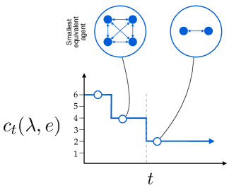
(a) Minimal Size

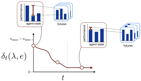
(b) Minimal Distortion

Figure 1: A cartoon visual of our two proposed definitions of convergence: (left) behavior convergence, and (right) performance convergence. Behavior convergence tracks the sequence, $\{c_{t}(\lambda,e)\}_{t=0}^{\infty}$, measuring the minimum number of states needed to produce the agent’s behavior from the current time step across all outcomes that could occur in the environment. Performance convergence tracks the sequence, $\{\delta_{t}(\lambda,e)\}_{t=0}^{\infty}$, measuring the maximum change in the agent’s performance across return visits to its agent states. The vertical dashed line indicates the time of convergence in each case: On the left, the agent’s minimal size has stopped decreasing, and on the right, the agent’s distortion has stopped decreasing.

The notion of convergence underlies many fundamental concepts in RL, and is part of the scientific community’s parlance. But what do we mean when we say that an agent has converged?

When we say some object that evolves over time converges, we tend to mean that we can characterize the evolution of the object as approaching a specific point. For instance, when we speak about the convergence results of Q-learning by Watkins & Dayan (1992), we mean that the limiting sequence of Q-values maintained by the algorithm arrives at a fixed point with probability one. Indeed, this is borrowing directly from the well-defined notions of the convergence of a sequence: One classical definition says roughly that a sequence of random variables, $X_{1},X_{2},\ldots$ converges to a number $z\in\mathbbm{R}$ just when, for all $\epsilon\in\mathbbm{R}_{>0}$, with probability one there exists a $t$ such that for all $n>t$, it holds that $|z-X_{n}|<\epsilon$. Naturally, there is a plurality of such notions, such as pointwise convergence or convergence in probability. We can apply these notions to any sequence generated by the interaction of the agent with the environment.

In typical models of the RL problem such as $k$-armed bandits or MDPs, the choice of the problem formulation immediately restricts our focus to sequences that are suggested by the presence of environment state: For instance, we might consider the agent’s choice of an action distribution over time (in the case of bandits, when there is only one environment state) or the agent’s choice of a policy over time (in the case of an MDP). We can imagine generalizing to POMDPs by simply asking whether the agent’s behavior or performance has converged relative to the POMDP’s hidden state. However, from the view focused on agents, it is less clear which sequence we might be interested in.

Ultimately, we will introduce two new fundamental definitions of an agent-environment pair that induce sequences (pictured in Figure 1), whose limits reflect the convergence of a bounded agent from two perspectives:

1. (Behavior) Minimal Size, $c_{t}(\lambda,e)$, given by Definition 3.1: A measurement of the smallest state space needed to produce the agent’s behavior across all realizable futures in the environment.

2. (Performance) Distortion, $\delta_{t}(\lambda,e)$, given by Definition 4.1: A measurement of the gap in the agent’s performance across future visits to the same agent state in the environment.

We next motivate and define each of these quantities in more detail. Our analysis reveals that the limit of each sequence exists for every $(\lambda,e)$ pair (Theorem 3.1, Theorem 4.2). In MDPs, we show these two measures are connected (Proposition 3.3, Proposition 4.3), which may explain why, historically, there was less pressure to draw the distinction between convergence in performance and behavior. However, in the most general settings, we show they are in fact distinct (Proposition 4.6).

3 Convergence in Behavior

We first explore convergence from the viewpoint of behavior. Intuitively, we might think an agent has converged in a bandit problem when the agent only pulls a single arm forever after. How might we generalize this intuition?

3.1 Limiting Size: $c_{\infty}(\lambda,e)$

Our first definition is built around the following perspective: An agent has converged in behavior in an environment when the minimal number of states needed to describe the agent’s future behaviors can no longer decrease. We focus around uniform convergence, in which agents converge in an environment uniformly across all realizable histories $\bar{\mathcal{H}}$, but note that alternative formulations are possible (and can be easily derived from ours).

To define this idea carefully, we introduce one new fundamental concept of an agent-environment pair: The number of states needed, in the limit, to reproduce the agent’s future behavior in the environment. First, let

$$\Lambda_{n}=\{\lambda\in\mathbbl{\Lambda}:|\lambda|=n\},$$ (3.1)

denote the set of agents operating over a state space of size $n\in\mathbbm{N}$. We define an agent’s minimal size at time $t\in\mathbbm{N}_{0}$ in terms of the size of the smallest agent that produces identical future behavior to $\lambda$ in $e$ as follows.

Definition 3.1.

The minimal size from time $\bm{t}$ of agent $\lambda$ in environment $e$ is denoted

$$c_{t}(\lambda,e)=\min\{n\in\mathbb{N}:\forall_{h\in\bar{\mathcal{H}}_{t:\infty}}\exists_{\lambda_{n}\in\Lambda_{n}}\forall_{h^{\prime}\in\acute{\mathcal{H}}}\ \lambda(hh^{\prime})=\lambda_{n}(hh^{\prime})\}.$$

So, given any time $t\in\mathbbm{N}_{0}$, we measure the minimal number of states needed to reproduce the agent’s behavior forever after in the environment. Intuitively, this number describes how compressed the agent could be, while still producing the same behavior in the current environment from the current time on. Notice that $c_{t}(\lambda,e)\leq|\lambda|$, as the agent cannot be both (i) minimal and, (ii) larger than its current size. Further observe that $c_{t}(\lambda,e)\geq 1$ by definition—we suppose the smallest agent has a single state by convention.

The minimal size from time $t$ produces a sequence, $\{c_{t}(\lambda,e)\}_{t=0}^{\infty}$, with which we can sensibly discuss the convergence of an agent. In particular, the limit of this sequence captures the minimal number of states needed to describe the agent’s behavior in the limit of interaction with $e$.

Definition 3.2.

The limiting size of agent $\lambda$ interacting with environment $e$ is defined as

$$c_{\infty}(\lambda,e)=\lim_{t\rightarrow\infty}c_{t}(\lambda,e).$$ (3.2)

We take the value of this limit to be capture to capture what it means for an agent’s behavior to converge. To see why, we next turn to the analysis of the limiting size.

3.2 Analysis: Behavior Convergence

The limiting size comes with several useful properties that strengthen its case as a convergence definition. All proofs are presented in the Appendix.

Theorem 3.1.

For every $(\lambda,e)$ pair:

1. The sequence $\{c_{t}(\lambda,e)\}_{t=0}^{\infty}$ is non-increasing.

2. $1\leq c_{t}(\lambda,e)\leq|\lambda|,\forall_{t\geq 0}$.

3. $c_{\infty}(\lambda,e)$ exists.

Hence, by point (c), we can sensibly talk about any agent’s limiting size in any given environment.

We further point out several special cases—when an agent is equivalent to a memoryless policy or a fixed $k$-th order policy, its limiting size must obey certain bounds. To be precise, we let,

$$\Pi_{\mathcal{O}}=\{\pi:\mathcal{O}\rightarrow\Delta(\mathcal{A})\},$$ (3.3)

denote the set of all memoryless policies.

Remark 3.2.

For every $(\lambda,e)$ pair:

1. If $\lambda$ is equivalent to a memoryless policy, $\pi_{\mathcal{O}}\in\Pi_{\mathcal{O}}$, then $c_{\infty}(\lambda,e)\leq|\mathcal{O}|$, in every environment.

2. If $\lambda$ is equivalent to a $k$-th order policy, $\pi:\mathcal{O}^{k}\rightarrow\Delta(\mathcal{A})$, then $c_{\infty}(\lambda,e)\leq|\mathcal{O}|^{k}$, in every environment.

This remark notes that, when an agent is equivalent to a memoryless policy, its limiting size will be upper bounded by the size of the observation space. More specifically, we next establish that the limiting size accommodates at least one simple view of convergence in bandits and MDPs in which an agent’s behavior eventually becomes uniformly equivalent to a distribution over actions (in bandits) or a memoryless policy (in MDPs).

Proposition 3.3.

The following two statements hold:

1. (Bandits) If an agent $\lambda$ uniformly converges in a $k$-armed bandit $e$ in the sense that,

   $$\exists_{t\in\mathbb{N}_{0}}\exists_{\rho\in\Delta(\mathcal{A})}\forall_{h\in\bar{\mathcal{H}}_{t:\infty}}\ \rho=\lambda(h),$$ (3.4)

   then $c_{\infty}(\lambda,e)=1$.

2. (MDPs) If an agent $\lambda$ uniformly converges in an MDP $e$ in the sense that,

   $$\exists_{t\in\mathbb{N}_{0}}\exists_{\pi_{\mathcal{O}}\in\Pi_{\mathcal{O}}}\forall_{hao\in\bar{\mathcal{H}}_{t:\infty}}\ \pi_{\mathcal{O}}(o)=\lambda(hao),$$ (3.5)

   then $c_{\infty}(\lambda,e)\leq|\mathcal{O}|$.

Thus, an agent’s minimal limiting size has an intuitive value in well-studied settings: In a bandit, a convergent agent eventually becomes a one-state agent; in an MDP, a convergent agent eventually becomes (at most) a $|\mathcal{O}|$-state agent. It is an open (and perhaps unanswerable) question as to what canonical agents converge to in more general environments, but the measure $c_{\infty}(\lambda,e)$ can give us some insight.

To summarize, we have introduced an agent’s limiting size as a quantity that reflects the convergence of an agent’s behavior in a given environment. In bandits and MDPs, the measure indicates the agent converges to a particular choice of distribution over actions, and a mapping from each environment state to a distribution over actions, respectively. In general, an agent’s behavior converges when its minimal size stops decreasing.

4 Convergence in Performance

We next explore the convergence of an agent’s performance, as studied in prior work in general RL (Lattimore & Hutter, 2011; Lattimore, 2014; Leike et al., 2016). Indeed, we are often interested in an agent’s asymptotic performance, or its rate of convergence to the asymptote (Fiechter, 1994; Szepesvári, 1997; Kearns & Singh, 1998). As we inspect learning curves in practice, it is common to say an agent has converged when the learning curve levels off. Moreover, reward or performance sequences induce a series of numbers over time, and thus can be readily mapped to classical accounts of the convergence of sequences.

4.1 Limiting Distortion: $\delta_{\infty}(\lambda,e)$

Recall that in an environment $e$ there is no explicit reference to state—only histories. How might we think of an agent’s performance converging? We could consider a strict approach that says an agent’s performance converges when it is constant across all future histories. This is much too strong, however, as it fails to accommodate relevant changes in performance that occur solely due to the change in history. For example, in the case that $e$ can be captured by an MDP (and thus, the observation is a sufficient statistic of reward, transitions, and performance), then surely we want to allow changes in performance as the agent changes between environment state. What happens when we no longer have an explicit reference to environment state?

As with the behavioral view, we find that bounded agents provide the needed structure—each bounded agent is comprised of a finite state space, $\mathcal{S}$. We can then define performance convergence relative to agent state by inspecting whether the agent’s performance changes across return visits to each of its own agent states. Intuitively, if the agent’s performance is the same every time it returns to the same agent state, then we say the agent has converged. We formally capture this notion through the limiting distortion of an agent-environment pair, which serves as the basis for our second definition of agent convergence.

To introduce this concept, we require extra notation to capture return visits to the same agent state. We are interested in realizable histories that can be subdivided, $hh^{\prime}$, such that the agent maps $h$ and $hh^{\prime}$ to the same internal agent state. We denote this set

$$\mathcal{H}^{\circ}_{t}=\ \{(h,h^{\prime})\in\mathcal{H}:\ hh^{\prime}\in\bar{\mathcal{H}}_{t:\infty}\ \wedge\ |h|\geq t,$$ (4.1)

$$\wedge\ |h^{\prime}|>0,$$

$$\wedge\ \vec{u}(h)=\vec{u}(hh^{\prime})\}.$$

Note that for all bounded agents, this set is non-empty for all environments $e\in{\mathcal{E}}$ and all times $t\in\mathbb{N}_{0}$.

Lemma 4.1.

$|\mathcal{H}_{t}^{\circ}|>0$ for any $(\lambda,e)$ pair and time $t\in\mathbb{N}_{0}$.

We can then consider the gap in the agent’s performance conditioned on the fact that the agent occupies the same agent state at two different times. This quantity, called distortion, analysed recently by Dong et al. under a more detailed decomposition of agent state (2022, Equations 5 & 6), is closely related to the degree of value error in aggregating states (Van Roy, 2006; Li et al., 2006) or histories (Majeed & Hutter, 2018; 2019; Majeed, 2021). We adapt these quantities in our notation as follows.

Definition 4.1.

The distortion from time $\bm{t}$ of $\lambda$ in $e$ is

$$\delta_{t}(\lambda,e)=\\ \sup_{(h,h^{\prime})\in\mathcal{H}^{\circ}_{t}}|v(\lambda,e\mid h)-v(\lambda,e\mid hh^{\prime})|.$$ (4.2)

Intuitively, the distortion of an agent expresses the largest gap in performance across situations in which the agent is at the same agent state. An agent with high distortion is one in which the agent will produce very different performance as it returns to the same agent state. On the other extreme, an agent with zero distortion is one in which the performance is constant every time the agent is at the same agent state. In this way, the distortion captures whether the agent-environment interaction is non-stationary in a way that is relevant to performance.

Using this measure, we introduce the limiting distortion, the central definition of this section.

Definition 4.2.

The limiting distortion of $\lambda$ in $e$ is

$$\delta_{\infty}(\lambda,e)=\lim_{t\rightarrow\infty}\delta_{t}(\lambda,e).$$ (4.3)

Roughly, $\delta_{\infty}$ measures how well an agent’s state can predict the agent’s own performance across all subsequent histories. This quantity will be zero just when, every time the agent visits one of its states, the factors of the environment that determine the agent’s performance are the same. Thus, the limiting distortion measures the degree of performance-relevant non-stationarity present in the indefinite interaction with the environment.

4.2 Analysis: Performance Convergence

To motivate this quantity as a meaningful reflection of an agent’s performance convergence, we show that the limiting distortion has the following properties.

Theorem 4.2.

For every $(\lambda,e)$ pair:

1. The sequence $\{\delta_{t}(\lambda,e)\}_{t=0}^{\infty}$ is non-increasing.

2. $0\leq\delta_{t}(\lambda,e)\leq(\mathrm{v}_{\mathrm{max}}-\mathrm{v}_{\mathrm{min}}),\forall_{t\geq 0}$.

3. $\delta_{\infty}(\lambda,e)$ exists.

Crucially, property (c) of Theorem 4.2 shows that the limiting distortion exists for every $(\lambda,e)$ pair. The relevant questions, then, are (i) the rate at which the agent reaches $\delta_{\infty}(\lambda,e)$ , and (ii) what the value $\delta_{\infty}(\lambda,e)$ actually is. We suggest that differing values of $\delta_{\infty}(\lambda,e)$ indicate a meaningful difference in the interaction stream produced by $\lambda$ and $e$—and thus, reflect the convergence of $\lambda$ in $e$. We motivate this intuition with the following results.

In standard settings, behavior and performance convergence tend to co-occur. That is, in an MDP, given an agent whose behavior converges in the sense of Proposition 3.3, that same agent’s performance also converges, as follows.

Proposition 4.3.

The following two statements hold:

1. (Bandits) If an agent $\lambda$ uniformly converges in a $k$-armed bandit $e$ in the sense that,

   $$\exists_{t\in\mathbb{N}_{0}}\exists_{\rho\in\Delta(\mathcal{A})}\forall_{h\in\bar{\mathcal{H}}_{t:\infty}}\ \rho=\lambda(h),$$ (4.4)

   then $\delta_{\infty}(\lambda,e)=0$.

2. (MDPs) If an agent $\lambda$ uniformly converges in an MDP $e$ in the sense that,

   $$\exists_{t\in\mathbb{N}_{0}}\exists_{\pi_{\mathcal{O}}\in\Pi_{\mathcal{O}}}\forall_{hao\in\bar{\mathcal{H}}_{t:\infty}}\ \pi_{\mathcal{O}}(o)=\lambda(hao),$$ (4.5)

   then $\delta_{\infty}(\lambda,e)=0$.

This result mirrors that of Proposition 3.3 on the behavioral side. Recall, however, that the style of convergence characterized by Equation 3.5 is restrictive, and will not necessarily accommodate the style of convergence of, say, tabular Q-learning; for many stochastic environments it is unlikely that there is a finite $t$ at which Q-learning is equivalent to a memoryless policy uniformly over all histories. To this end, we next provide a general result about the performance convergence of agents with a particular form.

Proposition 4.4.

Any $\lambda$ and MDP $e$ that satisfy

$$u(s,a,o)=u(s^{\prime},a^{\prime},o^{\prime})\ \Rightarrow\ o=o^{\prime},\hskip 22.76219pt\forall_{s,s^{\prime}\in\mathcal{S}},\forall_{a,a^{\prime}\in\mathcal{A}},\forall_{o,o^{\prime}\in\mathcal{O}},$$ (4.6)

ensure $\delta_{t}(\lambda,e)=0$ for all $t\in\mathbb{N}_{0}$, and thus, $\delta_{\infty}(\lambda,e)=0$.

Note that the condition of Equation 4.6 is satisfied for all bounded agents that always store the most recent observation in memory, as is typical of many agents we implement. In this sense, bounded implementations of Q-learning may ensure $\delta_{\infty}(\lambda,e)=0$. It is an open question as to whether we can design a version of bounded Q-learning that ensures convergence in MDPs in the sense of the main result of Watkins & Dayan (1992). For instance, it is unclear how to design an appropriate step-size annealing schedule with only finitely many agent states.

Conversely, when we consider the same exact kind of environment but impose further constraints on the agent, we find that the limiting distortion can be greater than zero.

Proposition 4.5.

There is a choice of MDP $e$ and bounded Q-learning $\lambda$ that yields $\delta_{\infty}(\lambda,e)>0$.

The contrast of Proposition 4.4 with Proposition 4.5 draws a distinction between the convergence of different agent-environment pairs. In particular, when the environment models an MDP, we saw that bounded agents that memorize the last observation satisfy $\delta_{\infty}(\lambda,e)=0$. However, when we consider a Q-learning agent with limitations to its representational capacity, we find it may be the case that $\delta_{\infty}(\lambda,e)>0$.

Lastly, we recall that by Proposition 3.3 and Proposition 4.3, behavioral and performance convergence tend to co-occur in traditional problems like MDPs. As a final point, we show that, in general environments, there are $(\lambda,e)$ pairs for which the time of behavior convergence is different from the time of performance convergence, thereby providing some formal support for treating these two views as distinct.

Proposition 4.6.

For any $(\lambda,e)$ pair and any choice of $\beta,\epsilon\in\mathbb{R}_{\geq 0}$ let

$$t_{\beta}(\lambda,e) =\min\{t\in\mathbb{N}_{0}:|c_{t}(\lambda,e)-c_{\infty}(\lambda,e)|\leq\beta\},$$

$$t_{\epsilon}(\lambda,e) =\min\{t\in\mathbb{N}_{0}:|\delta_{t}(\lambda,e)-\delta_{\infty}(\lambda,e)|\leq\epsilon\}.$$

Then, for $\beta=0$, $\epsilon=0$, there exists pairs $(\lambda,e)$ and $(\lambda^{\prime},e^{\prime})$ such that

$$t_{\epsilon}(\lambda,e)<t_{\beta}(\lambda,e),\hskip 11.38109ptt_{\beta}(\lambda^{\prime},e^{\prime})<t_{\epsilon}(\lambda^{\prime},e^{\prime}).$$ (4.7)

This result indicates that, in general, even when an agent’s limiting distortion has been reached, it does not mean that its limiting size has been reached, and vice versa. This tells a partial story as to why it is prudent to draw the concept of convergence in behavior and performance apart in more general environments. It is further worth noting that, in some environments, we suspect it is possible that $t_{\epsilon}$ may not exist, though $t_{\beta}$ is guaranteed to exist by definition of $c_{\infty}$.

5 Conclusion

The notion of convergence is central to many aspects of agency—for example, we are often interested in designing agents that converge to some fixed high-quality behavior. Similarly, the notion of learning is intimately connected to how we think about convergence: An agent that eventually converges is, in many cases, one that stops learning. In this paper we have presented a careful examination of the concept of convergence for bounded agents in an of RL that emphasizes agents rather than environments. We explored two perspectives on how to think about the convergence of a bounded agent operating in a general environment: from behavior (Definition 3.2), and from performance (Definition 4.2). We established simple properties of both formalisms, proved that they reflect some standard notions of convergence, and bear interesting relation to one another. We take these formalisms, definitions, and results to bring new clarity to a central concept of RL, and hope that this work can help us to better design, analyse, and understand learning agents.

The perspectives and definitions here introduced suggest a number of new pathways for the analysis and design of agents. For instance, both the limiting size and distortion of an agent can be useful guides for developing or evaluating the learning mechanisms that drive our agents; in some domains, we may explicitly want to build agents that converge in either sense, or to evaluate agents in environments that require a larger limiting size or distortion from its agents. Similarly, these quantities may suggest new ways to sharpen the problem we are ultimately interested in by focusing only on agents that have a minimal limiting size or distortion—as is likely the case of all agents of interest. Additionally, in future work, it would be useful to develop efficient algorithms that can estimate the limiting size or distortion of an actual agent-environment pair. Lastly, we emphasize that while behavior and performance are natural choices for a conception of convergence, we do not here discuss notions of convergence based around epistemic uncertainty (Lu et al., 2021), but acknowledge its potential significance for future work.

Acknowledgments

The authors are grateful to Mark Rowland for comments on a draft of the paper. We would also like to thank the attendees of the 2023 Barbados RL Workshop, as well as Elliot Catt, Will Dabney, Steven Hansen, Anna Harutyunyan, Joe Marino, Joseph Modayil, Remi Munos, Brendan O’Donoghue, Matt Overlan, Tom Schaul, Yunhao Tang, Shantanu Thakoor, and Zheng Wen for inspirational conversations.

Appendix A Appendix

We present each result and its associated proof in full detail, beginning with proofs of results presented in Section 3.

Theorem 3.1.

For every $(\lambda,e)$ pair, the following properties hold:

1. The sequence $\{c_{t}(\lambda,e)\}_{t=0}^{\infty}$ is non-increasing.

2. $1\leq c_{t}(\lambda,e)\leq|\lambda|,\forall_{t\geq 0}$.

3. $c_{\infty}(\lambda,e)$ exists.

Proof of Theorem 3.1..

We prove each property separately.

(a) The sequence $\{c_{t}(\lambda,e)\}_{t=0}^{\infty}$ is non-increasing.

Note that the set $\overline{\mathcal{H}}_{t:\infty}$ induces a sequence of sets $\overline{\mathcal{H}}_{0:\infty},\overline{\mathcal{H}}_{1:\infty},\ldots$ such that

$$\overline{\mathcal{H}}_{t+1:\infty}\subseteq\overline{\mathcal{H}}_{t:\infty},$$ (A.1)

for all $t\geq 0$. The non-increasing nature of the sequence $\{c_{t}(\lambda,e)\}_{t=0}^{\infty}$ holds by immediate consequence of this subset relation, as the $\sup$ ensures that

$$\sup\mathcal{X}_{t+1}\leq\sup\mathcal{X}_{t},$$

for countable sets $\mathcal{X}_{t+1}$ and $\mathcal{X}_{t}$ where $\mathcal{X}_{t+1}\subseteq\mathcal{X}_{t}$. Therefore, $c_{t+1}(\lambda,e)\leq c_{t}(\lambda,e)$ for all $t\geq 0$. ✓.

(b) $1\leq c_{t}(\lambda,e)\leq|\lambda|,\ \forall_{t\geq 0}$.

Second, note that the lower bound trivially holds since the smallest an agent can be is a single state (simply by convention—we could opt for the empty state space as the smallest agent, but this choice is arbitrary). Next, we note that the upper bound also holds in a straightforward way: The minimal state space size of the agent can’t be larger than the agent’s actual state space. ✓

(c) $c_{\infty}(\lambda,e)$ exists.

The property follows directly by consequence of the agent’s boundedness: The actual agent $\lambda$ uses a state space of some finite size, $b$. Thus, for every time $t$, in every environment, there is at least one $b\in\mathbbm{N}$, and one bounded agent that produces the same behavior as the agent: The agent itself. Therefore, by the non-increasing nature of the sequence, there must exist a point at which $c_{\infty}(\lambda,e)$ stops decreasing, due to the floor at the minimum possible state-space size of one. ✓

This completes the argument for all three statements, and thus completes the proof. ∎

Remark 3.2.

For every $(\lambda,e)$ pair:

1. If $\lambda$ is equivalent to a memoryless policy, $\pi_{\mathcal{O}}\in\Pi_{\mathcal{O}}$, then $c_{\infty}(\lambda,e)\leq|\mathcal{O}|$, in every environment.

2. If $\lambda$ is equivalent to a $k$-th order policy, $\pi:\mathcal{O}^{k}\rightarrow\Delta(\mathcal{A})$, then $c_{\infty}(\lambda,e)\leq|\mathcal{O}|^{k}$, in every environment.

Proof of Remark 3.2..

While (a) is clearly a special case of (b), we provide a proof of each result for the sake of clarity.

(a) If $\lambda$ is equivalent to a memoryless policy, then $c_{\infty}(\lambda,e)\leq|\mathcal{O}|$, in every environment.

To be precise, when we say an $\lambda$ is equivalent to a memoryless policy, we mean there is a choice of $\pi_{\mathcal{O}}\in\Pi_{\mathcal{O}}$ such that,

$$\lambda(h)=\pi_{\mathcal{O}}(h),\ \forall_{h\in\overline{\mathcal{H}}}.$$ (A.2)

Now that this term is clear, we see why the fact holds. The agent’s behavior can always be described by a process that sets its agent state to be the last observation, then acts according to the corresponding $\pi_{\mathcal{O}}$ from Equation A.2. That is, consider $\lambda^{\diamond}$ that (1) sets $\mathcal{S}=\mathcal{O}$, (2) sets $s$ = $o$, and (3) acts according to $\pi_{\mathcal{O}}^{\diamond}$,

$$\pi_{\mathcal{O}}^{\diamond}(s)=\pi_{\mathcal{O}}(o).$$

Clearly this agent only requires at most $|\mathcal{O}|$ states, and thus, $c_{\infty}(\lambda,e)\leq|\mathcal{O}|$. ✓

(b) If ${\vec{\lambda}}$ is equivalent to a $k$-th order policy, $\pi:\mathcal{O}^{k}\rightarrow\Delta(\mathcal{A})$, then $c_{\infty}(\lambda,e)\leq|\mathcal{O}|^{k}$, in every environment.

The reasoning is similar to point (3.). Let us first be precise: When we say the agent $\lambda$ is a $k$-th order policy, $\pi:\mathcal{O}^{k}\rightarrow\Delta(\mathcal{A})$, we mean the agent’s behavior can be described by some fixed function $\pi^{(k)}:\mathcal{O}^{k}\rightarrow\Delta(\mathcal{A})$ in every environment. That is, $\lambda=(\mathcal{S},s_{0},\pi,u)$ operates over some finite state space, and uses a policy $\pi:\mathcal{S}\rightarrow\Delta(\mathcal{A})$. But, this agent ensures there exists a $k$-th order policy $\pi^{(k)}$ such that, for any $t$, for every $h_{t}=a_{0}o_{1},\ldots,a_{t-2}o_{t-1}$,

$$\lambda(\cdot\mid h_{t})=\pi^{(k)}(\cdot\mid o_{t-k-1},\ldots,o_{t-2},o_{t-1}).$$

We note that handling the indices for the first observations where $t<k$ must be done carefully, but the reasoning remains the same.

Hence, we can define a new agent, $\lambda^{\diamond}=(\mathcal{S}^{\diamond},s_{0}^{\diamond},\pi^{\diamond},u^{\diamond})$, with $\mathcal{S}^{\diamond}=\mathcal{O}^{k}$, yielding:

$$\lambda(\cdot\mid h_{t})=\lambda^{\diamond}(\cdot\mid h_{t})=\pi^{\diamond}(\cdot\mid\underbrace{s_{t-1}^{\diamond}}_{o_{t-k-1},\ldots,o_{t-1}}).$$

By construction of $\lambda^{\diamond}$, the most states ever needed to mimic the behavior of $\lambda$ is $|\mathcal{O}|^{k}$.

We note that the relation is an inequality, $c_{\infty}(\lambda,e)\leq|\mathcal{O}|^{k}$, rather than a strict equality, as in some environments not every length $k$ sequence of observations may be required to produce the original agent’s behavior. ✓

This completes the argument for both statements. ∎

Proposition 3.3.

The following two statements hold:

1. (Bandits) If an agent $\lambda$ converges in a $k$-armed bandit $e$ in the sense that,

   $$\exists_{t\in\mathbb{N}_{0}}\exists_{\rho\in\Delta(\mathcal{A})}\forall_{h\in\overline{\mathcal{H}}_{t:\infty}}\ \rho=\lambda(h),$$ (A.3)

   then $c_{\infty}(\lambda,e)=1$.

2. (MDPs) If an agent $\lambda$ converges in an MDP $e$ in the sense that,

   $$\exists_{t\in\mathbb{N}_{0}}\exists_{\pi_{\mathcal{O}}\in\Pi_{\mathcal{O}}}\forall_{hao\in\overline{\mathcal{H}}_{t:\infty}}\ \pi_{\mathcal{O}}(o)=\lambda(hao),$$ (A.4)

   then $c_{\infty}(\lambda,e)\leq|\mathcal{O}|$.

Proof of Proposition 3.3..

We prove the two properties separately.

(a) (Bandits) If an agent $\lambda$ converges in a $k$-armed bandit $e$ in the sense that,

$$\exists_{t\in\mathbb{N}_{0}}\exists_{\rho\in\Delta(\mathcal{A})}\forall_{h\in\overline{\mathcal{H}}_{t:\infty}}\ \rho=\lambda(h),$$

then $c_{\infty}(\lambda,e)=1$.

We know by assumption that there is a time $t$ such that the agent’s chosen action distribution for all realizable histories is identical. Note that a fixed choice of action distribution can be captured by a memoryless policy $\pi_{\mathcal{O}}\in\Pi_{\mathcal{O}}$. Since $e$ is a $k$-armed bandit, we know there is only one observation, $|\mathcal{O}|=1$. Thus, by point (a) of Remark 3.2, we conclude $c_{\infty}(\lambda,e)\leq|\mathcal{O}|$, where $|\mathcal{O}|=1$. ✓

(b) (MDPs) If an agent $\lambda$ converges in an MDP $e$ in the sense that,

$$\exists_{t\in\mathbb{N}_{0}}\exists_{\pi_{\mathcal{O}}\in\Pi_{\mathcal{O}}}\forall_{hao\in\overline{\mathcal{H}}_{t:\infty}}\ \pi_{\mathcal{O}}(o)=\lambda(hao),$$

then $c_{\infty}(\lambda,e)\leq|\mathcal{O}|$.

The argument is similar to the previous point: We know by assumption that there is a time $t$ such that the agent’s behavior in all realizable histories is equivalent to some memoryless policy, $\pi_{\mathcal{O}}\in\Pi_{\mathcal{O}}$. By point (a) of Remark 3.2, we know that any agent that is equivalent to such a policy ensures $c_{\infty}(\lambda,e)\leq|\mathcal{O}|$. ✓

This completes the proof of both statements, and thus concludes the argument. ∎

Appendix B Section 4 Proofs: Convergence in Performance

We now present proofs of results from Section 4.

Lemma 4.1.

$|\mathcal{H}_{t}^{\circ}|>0$ for any $(\lambda,e)$ pair and time $t\in\mathbb{N}_{0}$.

Proof of Lemma 4.1..

The intuition is simple to state: All bounded agents must eventually return to at least one of their agent states.

In more detail, recall that in Equation 4.1 we define $\mathcal{H}^{\circ}_{t}$ to contain all history pairs $(h,h^{\prime})$ such that the following four conditions hold:

1. $hh^{\prime}\in\overline{\mathcal{H}}_{t:\infty}$,

2. $|h|\geq t$,

3. $|h|>0$.

4. $\vec{u}(h)=\vec{u}(hh^{\prime})$,

We now show that for any $(\lambda,e)$ pair and $t\in\mathbb{N}_{0}$, there will always be a pair $(h,h^{\prime})$ that satisfies all four properties.

(i) $hh^{\prime}\in\overline{\mathcal{H}}_{t:\infty}$.

Let us consider the first property. Recall that $\overline{\mathcal{H}}_{t:\infty}$ contains histories of length $t$ or greater that occur with non-zero probability from the interaction between $\lambda$ and $e$. By definition of this set, it is non-empty. ✓

(ii) $|h|\geq t$ and (iii) $|h^{\prime}|>0$.

Now, observe that by necessity some of the $(h,h^{\prime})$ pairs that satisfy the first condition, also satisfy the second and third conditions: Pick any realizable history from $\overline{\mathcal{H}}_{t:\infty}$ and there is a way to divide into pieces $h$ and $h^{\prime}$ such that $|h|\geq t$ and $|h|>0$. ✓

(iv) $\vec{u}(h)=\vec{u}(hh^{\prime})$.

Now, lastly, observe that some $(h,h^{\prime})$ pairs that satisfy these three conditions must also ensure that the agent occupies the same agent state after experiencing $h$ and $hh^{\prime}$. That is, that $\vec{u}(h)=\vec{u}(hh^{\prime})$. If this were not the case, then for all such history pairs $h$ and $h^{\prime}$ that satisfy conditions (i, ii, iii), the agent would have to occupy a different agent state across $h$ and $hh^{\prime}$. But then as the length of $h$ and $hh^{\prime}$ go to infinity, the agent will occupy infinitely many different agent states, which contradicts its boundedness. ✓

This completes the argument for each of the four properties, and thus completes the proof. ∎

Theorem 4.2.

For every $(\lambda,e)$ pair:

1. The sequence $\{\delta_{t}(\lambda,e)\}_{t=0}^{\infty}$ is non-increasing.

2. $0\leq\delta_{t}(\lambda,e)\leq(\mathrm{v}_{\mathrm{max}}-\mathrm{v}_{\mathrm{min}}),\forall_{t\geq 0}$.

3. $\delta_{\infty}(\lambda,e)$ exists.

Proof of Theorem 4.2..

We prove each property separately.

(a) The sequence $\{\delta_{t}(\lambda,e)\}_{t=0}^{\infty}$ is non-increasing.

Note that the set $\mathcal{H}^{\circ}_{t}$ induces a sequence of non-empty sets $\mathcal{H}^{\circ}_{0}$, $\mathcal{H}^{\circ}_{1}\ldots$ such that

$$\mathcal{H}^{\circ}_{t+1}\subseteq\mathcal{H}^{\circ}_{t},$$ (B.1)

for all $t\geq 0$. Further, Lemma 4.1 ensures each of these sets are non-empty. The non-increasing nature of the sequence $\{\delta_{t}(\lambda,e)\}_{t=0}^{\infty}$ holds by immediate consequence of this subset relation, as the $\sup$ ensures that

$$\sup\mathcal{X}_{t+1}\leq\sup\mathcal{X}_{t},$$

for countable sets $\mathcal{X}_{t+1}$ and $\mathcal{X}_{t}$ where $\mathcal{X}_{t+1}\subseteq\mathcal{X}_{t}$. Therefore, $\delta_{t+1}(\lambda,e)\leq\delta_{t}(\lambda,e)$ for all $t\geq 0$. ✓.

(b) $0\leq\delta_{t}(\lambda,e)\leq(\mathrm{v}_{\mathrm{max}}-\mathrm{v}_{\mathrm{min}}),\ \forall_{t\geq 0}$.

The lower bound holds as a direct consequence of the presence of the absolute value in Equation 4.2. The upper bound holds as a direct consequence of the boundedness of the function $v$. ✓

(c) The quantity $\delta_{\infty}(\lambda,e)$ exists for every agent-environment pair.

First we expand the definition of $\delta_{\infty}(\lambda,e)$,

$$\delta_{\infty}(\lambda,e)$$ (B.2)

$$=\lim_{t\rightarrow\infty}\delta_{t}(\lambda,e)$$

$$=\lim_{t\rightarrow\infty}\sup_{(h,h^{\prime})\in\mathcal{H}^{\circ}_{t}}|v(\lambda,e\mid h)-v(\lambda,e\mid hh^{\prime})|.$$

Note that the sequence $\{\delta_{t}(\lambda,e)\}_{t=0}^{\infty}$ is bounded by property (b): It is bounded below by 0 and above by $(\mathrm{v}_{\mathrm{max}}-\mathrm{v}_{\mathrm{min}})$. Thus, since the $\limsup$ of a bounded sequence always exists, we conclude that $\delta_{\infty}(\lambda,e)$ always exists. ✓

This completes the argument for all three statements, and thus completes the proof. ∎

Proposition 4.3.

The following two statements hold:

1. (Bandits) If an agent $\lambda$ uniformly converges in a $k$-armed bandit $e$ in the sense that,

   $$\exists_{t\in\mathbb{N}_{0}}\exists_{\rho\in\Delta(\mathcal{A})}\forall_{h\in\overline{\mathcal{H}}_{t:\infty}}\ \rho=\lambda(h),$$ (B.3)

   then $\delta_{\infty}(\lambda,e)=0$.

2. (MDPs) If an agent $\lambda$ uniformly converges in an MDP $e$ in the sense that,

   $$\exists_{t\in\mathbb{N}_{0}}\exists_{\pi_{\mathcal{O}}\in\Pi_{\mathcal{O}}}\forall_{hao\in\overline{\mathcal{H}}_{t:\infty}}\ \pi_{\mathcal{O}}(o)=\lambda(hao),$$ (B.4)

   then $\delta_{\infty}(\lambda,e)=0$.

Proof of Proposition 4.3..

We prove the result for the MDP case, and since bandits are a clear instance of MDPs and the memoryless policies on $\mathcal{O}=\{o_{1}\}$ are equivalent to the set $\Delta(\mathcal{A})$, it follows that $\delta_{\infty}(\lambda,e)=0$ for bandits, too.

(b) (MDPs) If an agent $\lambda$ converges in an MDP $e$ in the sense that,

$$\exists_{t\in\mathbb{N}_{0}}\exists_{\pi_{\mathcal{O}}\in\Pi_{\mathcal{O}}}\forall_{hao\in\overline{\mathcal{H}}_{t:\infty}}\ \pi_{\mathcal{O}}(o)=\lambda(hao),$$ (B.5)

then $\delta_{\infty}(\lambda,e)=0$.

By Equation B.5, we know that there is a time $t$ at which the agent will act according to a fixed memoryless policy forever after.

Let us consider some time $t^{\prime}>t$, and recall that the distortion at time $t^{\prime}$ is given by,

$$\delta_{t^{\prime}}(\lambda,e)=\sup_{(h,h^{\prime})\in\mathcal{H}^{\circ}_{t^{\prime}}}|v(\lambda,e\mid h)-v(\lambda,e\mid hh^{\prime})|>0.$$

Let us consider what happens at the history pair, $h$ and $hh^{\prime}$. Since $(h,h^{\prime})\in\mathcal{H}^{\circ}_{t^{\prime}}$, we know that the agent occupies the same agent state at both $h$ and $hh^{\prime}$. Further, since $t^{\prime}>t$, we know that the agent is equivalent to some memoryless policy at both $h$ and $hh^{\prime}$, and will thus make the same choice of action distribution at both $h$ and $hh^{\prime}$. Therefore, the agent will act in an equivalent manner at both $h$ and $hh^{\prime}$. But this is also true for all subsequent realizable histories, and thus, the agent’s performance must be equivalent at both $h$ and $hh^{\prime}$. We conclude that $v(\lambda,e\mid h)=v(\lambda,e\mid hh^{\prime})$, and thus, for all $t^{\prime}>t$,

$$\delta_{t}(\lambda,e)=0.$$ (B.6)

By the non-increasing nature of $\{\delta_{t}(\lambda,e)\}_{t=0}^{\infty}$, we conclude $\delta_{\infty}(\lambda,e)=0$. ∎

Proposition 4.4.

Any $\lambda$ and MDP $e$ that satisfy

$$u(s,a,o)=u(s^{\prime},a^{\prime},o^{\prime})\ \Rightarrow\ o=o^{\prime},\hskip 22.76219pt\forall_{s,s^{\prime}\in\mathcal{S}},\forall_{a,a^{\prime}\in\mathcal{A}},\forall_{o,o^{\prime}\in\mathcal{O}},$$ (B.7)

ensure $\delta_{t}(\lambda,e)=0$ for all $t\in\mathbb{N}_{0}$, and thus, $\delta_{\infty}(\lambda,e)=0$.

Proof of Proposition 4.4..

Consider a fixed but arbitrary pair $(\lambda,e)$ such that Equation B.7 is satisfied.

Then, for arbitrary $t$, consider the performance of this agent at two histories $h$ and $hh^{\prime}$, where $(h,h^{\prime})\in\mathcal{H}^{\circ}_{t}$. Again we know such a pair exists by Lemma 4.1. Further, we know by definition of $\mathcal{H}^{\circ}_{t}$ that the agent will occupy the same agent state after experiencing $h$ and $hh^{\prime}$. That is, letting

$$h =\ldots ao,\hskip 22.76219pts=\vec{u}(h),$$

$$h^{\prime} =\ldots a^{\prime}o^{\prime},\hskip 17.07164pts^{\prime}=\vec{u}(h^{\prime}),$$

it follows that

$$\vec{u}(s,a,o)=\vec{u}(s^{\prime},a^{\prime},o^{\prime}).$$ (B.8)

By assumption, we supposed that the given agent and environment satisfy Equation B.7, and therefore, together with Equation B.8, it follows that $o=o^{\prime}$. But, since $e$ is an MDP, anytime the MDP occupies the same MDP-state and the agent occupies the same agent-state, the resulting performance will be the same. Thus, $v(\lambda,e\mid h)=v(\lambda,e\mid hh^{\prime})$.

Since the time $t$ and history pair $(h,h^{\prime})$ were chosen arbitrarily, we know that

$$v(\lambda,e\mid h)=v(\lambda,e\mid hh^{\prime}),$$

holds for all $t$ and $h,h^{\prime}\in\mathcal{H}^{\circ}_{t}$. Therefore, for all $t\in\mathbbm{N}_{0}$

$$\delta_{t}(\lambda,e) =\sup_{(h,h^{\prime})\in\mathcal{H}^{\circ}_{t}}|v(\lambda,e\mid h)-\underbrace{v(\lambda,e\mid hh^{\prime})}_{=v(\lambda,e\mid h)}|,$$

$$=\sup_{(h,h^{\prime})\in\mathcal{H}^{\circ}_{t}}|v(\lambda,e\mid h)-v(\lambda,e\mid h)|,$$

$$=0,$$

and hence, $\delta_{\infty}(\lambda,e)=0$. ∎

Proposition 4.5.

There is a choice of MDP $e$ and bounded Q-learning $\lambda$ that yields $\delta_{\infty}(\lambda,e)>0$.

Proof of Proposition 4.5..

For concreteness, we describe the agent and environment in more detail, but note that there is a neighborhood of such choices for which the same result holds. For simplicity, we let $v$ capture the expected myopic reward (so discounted return with $\gamma=0$). The same result extends for other settings of $\gamma$, but the argument is simplest in the myopic case.

The MDP $e$ is as follows.

1. The interface is defined as:

   $$\mathcal{O}=\{o_{1},o_{2}\},\hskip 17.07164pt\mathcal{A}=\{a_{\mathrm{move}},a_{\mathrm{stay}}\}.$$

   Thus, since the environment $e$ is an MDP, we understand the MDP to have two states defined by the two observations $\{o_{1},o_{2}\}$. We refer to these as MDP states throughout the proof.

2. The MDP’s transition function is defined as a deterministic function where $a_{\mathrm{move}}$ moves the agent to the other state, while $a_{\mathrm{stay}}$ causes the agent to stay in the same state.

3. The MDP’s reward function is as follows:

   $$r(oao^{\prime})=\begin{cases}-1&o=o_{1},\\ +1&\text{otherwise}.\\ \end{cases}$$ (B.9)

The agent is as follows.

1. The $\lambda$ is an instance of tabular Q-Learning with $\varepsilon$-greedy exploration that experiences every $(o,a)$ pair infinitely often.

2. Additionally, the agent $\lambda$ is bounded in that it has finitely many agent states. While there is a vast space of ways to make such an agent bounded, we choose to consider the case where the agent state is comprised of three quantities, $s=(Q_{t},\alpha_{t},\varepsilon_{t})$, where $Q_{t}:\mathcal{O}\times\mathcal{A}\rightarrow[\mathrm{v}_{\mathrm{min}},\mathrm{v}_{\mathrm{max}}]$ is the Q function, $\alpha_{t}\in[0,1]$ is the time-dependent step size, and $\varepsilon_{t}\in[0,1]$ is the time-dependent exploration parameter. Note that due to the boundedness of the agent, it can only have finitely many choices of $\alpha_{t}$ and $\epsilon_{t}$. Notice that as a result of this boundedness, it is an open question as to whether the precise conditions needed for Q-learning convergence in the classical sense will go through.

3. Lastly, the agent violates Equation B.7—The agent does not store its Q function as an exact function of the MDP’s state, $o\in\mathcal{O}$, but rather, the agent’s state-update function collapses $o_{1}$ and $o_{2}$ to a single Q function expressing the expected discounted return of $a_{\mathrm{move}},a_{\mathrm{stay}}$.

Now, we show that the pair defined above satisfies $\delta_{\infty}(\lambda,e)>0$. We do so through two points. First, we show that for arbitrarily chosen $t$, there is a valid history pair $(h,h^{\prime})\in\mathcal{H}^{\circ}_{t}$ where $h$ ends in $o_{1}$ and $h^{\prime}$ ends in $o_{2}$, and (2) that the performance $v(\lambda,e\mid h)\neq v(\lambda,e\mid hh^{\prime})$.

(1) For any $t\in\mathbb{N}$, there is a valid $(h,h^{\prime})\in\mathcal{H}^{\circ}_{t}$.

Consider a fixed but arbitrary time $t\in\mathbb{N}$, and a history pair, $(h,h^{\prime})\in\mathcal{H}^{\circ}_{t}$. Recall that this pair ensures that (1) $|h|\geq t$, (2) Both $h$ and $hh^{\prime}$ occur with non-zero probability via the interaction of $\lambda$ and $e$, and (3) The agent occupies the same agent state in $h$ and $hh^{\prime}$. Further, we require that $h$ ends in $o_{1}$, and $h^{\prime}$ ends in $o_{2}$. To see that such a history pair will exist for the chosen $t\in\mathbb{N}$, recall first that by assumption in point ($\lambda$.i), Q-learning will experience every $(o,a)$ pair infinitely often. By the agent’s boundedness in point ($\lambda$.i) together with Lemma 4.1 ensures that $|\mathcal{H}^{\circ}_{t}|\geq 0$. Next, by point ($\lambda.iii$), the agent is insensitive to the latest observation emitted, and so can occupy the same agent state between $h$ and $hh^{\prime}$, even when $h$ ends in $o_{1}$ and $h^{\prime}$ ends in $o_{2}$. For example, let $h=o_{1}a\ldots o_{1}ao_{2}$, and $h^{\prime}=ao_{2}$. Note that $r(h)=r(o_{1}ao_{1})=+1$, and note that $r(hh^{\prime})=r(o_{1}ao_{2})=+1$. Therefore the reward stream will not change the agent’s internal state, and thus $\vec{u}(h)=\vec{u}(hh^{\prime})$. ✓

(2) $v(\lambda,e\mid h)\neq v(\lambda,e\mid hh^{\prime})$.

Next notice that for this chosen $(h,h^{\prime})$ pair from step (1), the performance $v(\lambda,e\mid h)\neq v(\lambda,e\mid hh^{\prime})$. To see why, observe that in history $h$, the agent occupies MDP state $o_{1}$, and thus, the subsequent reward is guaranteed to be $+1$ by Equation B.9. Conversely, in history $hh^{\prime}$, the agent occupies MDP state $o_{2}$, and so the next reward receives is guaranteed to be $-1$ by Equation B.9. Since we assumed $\gamma=0$, it follows that $v(\lambda,e\mid h)\neq v(\lambda,e\mid hh^{\prime})$ and consequently, $\delta_{t}(\lambda,e)>0$. ✓

Since $t$ was chosen arbitrarily, we note that the above property holds for all $t\in\mathbb{N}$, and therefore,

$$\lim_{t\rightarrow\infty}\delta_{t}(\lambda,e)>0.\qed$$

Proposition 4.6.

For any $(\lambda,e)$ pair and any choice of $\beta,\epsilon\in\mathbb{R}_{\geq 0}$ let,

$$t_{\beta}(\lambda,e) =\min\{t\in\mathbb{N}_{0}:|c_{t}(\lambda,e)-c_{\infty}(\lambda,e)|\leq\beta\},$$

$$t_{\epsilon}(\lambda,e) =\min\{t\in\mathbb{N}_{0}:|\delta_{t}(\lambda,e)-\delta_{\infty}(\lambda,e)|\leq\epsilon\}.$$

Then, for $\beta=0$, $\epsilon=0$, there exists pairs $(\lambda,e)$ and $(\lambda^{\prime},e^{\prime})$ such that

$$t_{\epsilon}(\lambda,e)<t_{\beta}(\lambda,e),\hskip 11.38109ptt_{\beta}(\lambda^{\prime},e^{\prime})<t_{\epsilon}(\lambda^{\prime},e^{\prime}).$$ (B.10)

Proof of Proposition 4.6..

We construct two examples $(\lambda,e)$ where the time of performance convergence is different from the time of behavior convergence.

(a) Example 1: There exists a $(\lambda,e)$ such that $t_{\epsilon}(\lambda,e)<t_{\beta}(\lambda,e).$

We construct the example as follows. Let:

• $\lambda$ denote a single state agent that plays the same action at every round of interaction,

• $e$ denote an environment that produces $r(h_{t})=0$ for any history when $t>10$, but $r(h_{t})=1$ for all histories where $t\geq 10$,

• And, the performance $v(\lambda,e\mid h)$ produces the reward received only in the next time step following $h$, for any $h$.

Thus, since $\lambda$ only has a single state, we know $c_{0}(\lambda,e)=c_{\infty}(\lambda,e)=1$, and there $t_{\epsilon}=0$.

Conversely, we can see that $\delta_{0}(\lambda,e)=1$ whereas $\delta_{10}(\lambda,e)=\delta_{\infty}(\lambda,e)=0$, as the agent’s performance is zero at $h_{0}$, but the agent’s performance will be 1 for any $h_{0}h^{\prime}$ where $|h^{\prime}|\geq 10$. Thus, since $t_{\epsilon}=0$ and $t_{\beta}=10$, we conclude $t_{\epsilon}<t_{\beta}$. ✓

(b) Example 2: There exists a $(\lambda,e)$ such that $t_{\beta}(\lambda,e)<t_{\epsilon}(\lambda,e).$

Consider an environment with a constant reward function, $r(h)=0,\ \forall_{h\in\mathcal{H}}$. Then, by immediate consequence, $\delta_{0}(\lambda,e)=\delta_{t}(\lambda,e)=\delta_{\infty}(\lambda,e)=0,\ \forall_{t\geq 0}$. Thus, $t_{\epsilon}=0$ for any agent in this environment.

Now we construct an agent for which the time of behaviour convergence $t_{\beta}(\lambda,e)>0$. Observe that this is true of an agent that switches between two agent states for the first ten time steps, choosing a different action in each state. Then, at time step $t=10$, the agent sticks with a single state and choice of action forever after. Consequently, we see that the agent requires two states to produce its behavior up until time $t=10$, at which time the agent only requires one state. Therefore, $c_{0}(\lambda,e)=2$, but $c_{10}(\lambda,e)=c_{\infty}(\lambda,e)=1$. Hence, $t_{\beta}(\lambda,e)=10$, whereas $t_{\epsilon}(\lambda,e)=0$, and so $t_{\epsilon}<t_{\beta}$. ✓

This completes the proof of both conditions, and we conclude. ∎

References

- Auer et al. (2008) Peter Auer, Thomas Jaksch, and Ronald Ortner. Near-optimal regret bounds for reinforcement learning. Advances in Neural Information Processing Systems, 2008.
- Azar et al. (2017) Mohammad Gheshlaghi Azar, Ian Osband, and Rémi Munos. Minimax regret bounds for reinforcement learning. In Proceedings of the International Conference on Machine Learning, 2017.
- Bellman (1957) Richard Bellman. A Markovian decision process. Journal of Mathematics and Mechanics, pp. 679–684, 1957.
- Bowling et al. (2023) Michael Bowling, John D. Martin, David Abel, and Will Dabney. Settling the reward hypothesis. In Proceedings of the International Conference on Machine Learning, 2023.
- Bradtke & Barto (1996) Steven J Bradtke and Andrew G Barto. Linear least-squares algorithms for temporal difference learning. Machine learning, 22(1):33–57, 1996.
- Brafman & Tennenholtz (2002) Ronen I Brafman and Moshe Tennenholtz. R-max-a general polynomial time algorithm for near-optimal reinforcement learning. Journal of Machine Learning Research, 3(Oct):213–231, 2002.
- Calandriello et al. (2014) Daniele Calandriello, Alessandro Lazaric, and Marcello Restelli. Sparse multi-task reinforcement learning. Advances in neural information processing systems, 2014.
- Cassandra et al. (1994) Anthony R. Cassandra, Leslie Pack Kaelbling, and Michael L. Littman. Acting optimally in partially observable stochastic domains. In Proceedings of the AAAI Conference on Artificiall Intelligence, 1994.
- Cherniak (1990) Christopher Cherniak. Minimal rationality. MIT Press, 1990.
- Cohen et al. (2019) Michael K Cohen, Elliot Catt, and Marcus Hutter. A strongly asymptotically optimal agent in general environments. arXiv preprint arXiv:1903.01021, 2019.
- Diuk et al. (2008) Carlos Diuk, Andre Cohen, and Michael L Littman. An object-oriented representation for efficient reinforcement learning. In Proceedings of the International conference on Machine learning, 2008.
- Dong et al. (2022) Shi Dong, Benjamin Van Roy, and Zhengyuan Zhou. Simple agent, complex environment: Efficient reinforcement learning with agent states. Journal of Machine Learning Research, 23(255):1–54, 2022.
- Fazel et al. (2018) Maryam Fazel, Rong Ge, Sham Kakade, and Mehran Mesbahi. Global convergence of policy gradient methods for the linear quadratic regulator. In Proceedings of the International Conference on Machine Learning, 2018.
- Fiechter (1994) Claude-Nicolas Fiechter. Efficient reinforcement learning. In Proceedings of the Conference on Computational Learning Theory, 1994.
- Gordon (2000) Geoffrey J Gordon. Reinforcement learning with function approximation converges to a region. In Advances in Neural Information Processing Systems, 2000.
- Griffiths et al. (2015) Thomas L Griffiths, Falk Lieder, and Noah D Goodman. Rational use of cognitive resources: Levels of analysis between the computational and the algorithmic. Topics in cognitive science, 7(2):217–229, 2015.
- Harutyunyan (2020) Anna Harutyunyan. What is an agent? http://anna.harutyunyan.net/wp-content/uploads/2020/09/What_is_an_agent.pdf, 2020.
- Hutter (2000) Marcus Hutter. A theory of universal artificial intelligence based on algorithmic complexity. arXiv preprint cs/0004001, 2000.
- Hutter (2002) Marcus Hutter. Self-optimizing and Pareto-optimal policies in general environments based on Bayes-mixtures. In Proceedings of the International Conference on Computational Learning Theory, 2002.
- Hutter (2004) Marcus Hutter. Universal artificial intelligence: Sequential decisions based on algorithmic probability. Springer Science & Business Media, 2004.
- Icarte et al. (2022) Rodrigo Toro Icarte, Toryn Q Klassen, Richard Valenzano, and Sheila A McIlraith. Reward machines: Exploiting reward function structure in reinforcement learning. Journal of Artificial Intelligence Research, 73:173–208, 2022.
- Jaksch et al. (2010) Thomas Jaksch, Ronald Ortner, and Peter Auer. Near-optimal regret bounds for reinforcement learning. Journal of Machine Learning Research, 11(Apr):1563–1600, 2010.
- Jin et al. (2020) Chi Jin, Zhuoran Yang, Zhaoran Wang, and Michael I Jordan. Provably efficient reinforcement learning with linear function approximation. In Proceedings of the Conference on Learning Theory, 2020.
- Kaelbling et al. (1996) Leslie Pack Kaelbling, Michael L. Littman, and Andrew W. Moore. Reinforcement learning: A survey. Journal of Artificial Intelligence Research, pp. 237–285, 1996.
- Kearns & Koller (1999) Michael Kearns and Daphne Koller. Efficient reinforcement learning in factored MDPs. In Proceedings of the International Joint Conference on Artificial Intelligence, 1999.
- Kearns & Singh (1998) Michael Kearns and Satinder Singh. Finite-sample convergence rates for Q-learning and indirect algorithms. Advances in Neural Information Processing Systems, 1998.
- Kearns & Singh (2002) Michael Kearns and Satinder Singh. Near-optimal reinforcement learning in polynomial time. Machine learning, 49(2-3):209–232, 2002.
- Konidaris (2006) George Konidaris. A framework for transfer in reinforcement learning. In ICML Workshop on Structural Knowledge Transfer for Machine Learning, 2006.
- Konidaris & Barto (2006) George Konidaris and Andrew Barto. Autonomous shaping: Knowledge transfer in reinforcement learning. In Proceedings of the International Conference on Machine Learning, 2006.
- Konidaris & Barto (2007) George Konidaris and Andrew Barto. Building portable options: Skill transfer in reinforcement learning. In Proceedings of the International Joint Conference on Artificial Intelligence, 2007.
- Lattimore (2014) Tor Lattimore. Theory of general reinforcement learning. PhD thesis, The Australian National University, 2014.
- Lattimore & Hutter (2011) Tor Lattimore and Marcus Hutter. Asymptotically optimal agents. In Proceedings of the International Conference on Algorithmic Learning Theory, 2011.
- Lattimore et al. (2013) Tor Lattimore, Marcus Hutter, and Peter Sunehag. The sample-complexity of general reinforcement learning. In Proceedings of the International Conference on Machine Learning, 2013.
- Leike (2016) Jan Leike. Nonparametric general reinforcement learning. PhD thesis, The Australian National University, 2016.
- Leike et al. (2016) Jan Leike, Tor Lattimore, Laurent Orseau, and Marcus Hutter. Thompson sampling is asymptotically optimal in general environments. In Proceedings of the Conference on Uncertainty in Artificial Intelligence, 2016.
- Lewis et al. (2014) Richard L Lewis, Andrew Howes, and Satinder Singh. Computational rationality: Linking mechanism and behavior through bounded utility maximization. Topics in cognitive science, 6(2):279–311, 2014.
- Li et al. (2006) Lihong Li, Thomas J. Walsh, and Michael L. Littman. Towards a unified theory of state abstraction for MDPs. In Proceedings of the International Symposium on Artificial Intelligence and Mathematics, 2006.
- Lu et al. (2021) Xiuyuan Lu, Benjamin Van Roy, Vikranth Dwaracherla, Morteza Ibrahimi, Ian Osband, and Zheng Wen. Reinforcement learning, bit by bit. arXiv preprint arXiv:2103.04047, 2021.
- Majeed (2021) Sultan J Majeed. Abstractions of general reinforcement Learning. PhD thesis, The Australian National University, 2021.
- Majeed & Hutter (2018) Sultan J. Majeed and Marcus Hutter. On Q-learning convergence for non-Markov decision processes. In Proceedings of the International Joint Conference on Artificial Intelligence, 2018.
- Majeed & Hutter (2019) Sultan Javed Majeed and Marcus Hutter. Performance guarantees for homomorphisms beyond Markov decision processes. In Proceedings of the AAAI Conference on Artificial Intelligence, 2019.
- McCallum (1996) Andrew Kachites McCallum. Reinforcement learning with selective perception and hidden state. PhD thesis, 1996.
- Mnih et al. (2015) Volodymyr Mnih, Koray Kavukcuoglu, David Silver, Andrei A. Rusu, Joel Veness, Marc G. Bellemare, Alex Graves, Martin Riedmiller, Andreas K. Fidjeland, Georg Ostrovski, Stig Petersen, Charles Beattie, Amir Sadik, Ioannis Antonoglou, Helen King, Dharshan Kumaran, Daan Wierstra, Shane Legg, and Demis Hassabis. Human-level control through deep reinforcement learning. Nature, 518(7540):529–533, 2015.
- Ortega (2011) Pedro Alejandro Ortega. A unified framework for resource-bounded autonomous agents interacting with unknown environments. PhD thesis, University of Cambridge, 2011.
- Puterman (2014) Martin L Puterman. Markov Decision Processes: Discrete Stochastic Dynamic Programming. John Wiley & Sons, 2014.
- Puterman & Brumelle (1979) Martin L. Puterman and Shelby L. Brumelle. On the convergence of policy iteration in stationary dynamic programming. Mathematics of Operations Research, 4(1):60–69, 1979.
- Russell & Subramanian (1994) Stuart J Russell and Devika Subramanian. Provably bounded-optimal agents. Journal of Artificial Intelligence Research, 2:575–609, 1994.
- Sallans & Hinton (2004) Brian Sallans and Geoffrey E Hinton. Reinforcement learning with factored states and actions. The Journal of Machine Learning Research, 5:1063–1088, 2004.
- Schrittwieser et al. (2020) Julian Schrittwieser, Ioannis Antonoglou, Thomas Hubert, Karen Simonyan, Laurent Sifre, Simon Schmitt, Arthur Guez, Edward Lockhart, Demis Hassabis, Thore Graepel, et al. Mastering atari, Go, chess and shogi by planning with a learned model. Nature, 588(7839):604–609, 2020.
- Simon (1955) Herbert A Simon. A behavioral model of rational choice. The quarterly journal of economics, 69(1):99–118, 1955.
- Singh et al. (2000) Satinder Singh, Tommi Jaakkola, Michael L. Littman, and Csaba Szepesvári. Convergence results for single-step on-policy reinforcement-learning algorithms. Machine learning, 38(3):287–308, 2000.
- Strehl et al. (2009) Alexander L. Strehl, Lihong Li, and Michael L. Littman. Reinforcement learning in finite MDPs: PAC analysis. Journal of Machine Learning Research, 10:2413–2444, 2009.
- Sutton & Barto (2018) Richard S. Sutton and Andrew G. Barto. Reinforcement Learning: An Introduction. MIT Press, 2018.
- Sutton et al. (1999) Richard S Sutton, David McAllester, Satinder Singh, and Yishay Mansour. Policy gradient methods for reinforcement learning with function approximation. Advances in neural information processing systems, 1999.
- Szepesvári (1997) Csaba Szepesvári. The asymptotic convergence-rate of Q-learning. Advances in Neural Information Processing Systems, 1997.
- Todd & Gigerenzer (2012) Peter M Todd and Gerd Ed Gigerenzer. Ecological rationality: Intelligence in the world. Oxford University Press, 2012.
- Van Roy (2006) Benjamin Van Roy. Performance loss bounds for approximate value iteration with state aggregation. Mathematics of Operations Research, 31(2):234–244, 2006.
- Watkins & Dayan (1992) Christopher J.C.H. Watkins and Peter Dayan. -learning. Machine learning, 8(3-4):279–292, 1992.