Adiabatic or Non-Adiabatic? Unraveling the Nature of Initial Conditions in the Cosmological Gravitational Wave Background

Abstract

The non-thermal nature of the stochastic gravitational-wave background of cosmological origin (CGWB) poses a challenge in defining the initial conditions for the graviton overdensity. Specifically, the adiabatic initial condition, which holds for Cosmic Microwave Background (CMB) photons, is not guaranteed a priori for the primordial GWs. In this letter, we compute the initial conditions for the cosmological background generated by quantum fluctuations of the metric during inflation. Our analysis reveals that adiabatic initial conditions are no longer valid. The violation of adiabaticity arises from the presence of independent tensor perturbations during inflation, which behave as two extra fields that affect the standard single-clock argument. Since the energy density of the CGWB is subdominant compared to ordinary matter, gravitational radiation plays a negligible role in Einstein’s equations. Therefore, the only way to compute the initial conditions is to perturb the energy-momentum tensor defined in terms of the gravitational strain. A direct consequence of our finding is that the initial conditions from inflation enhance the total CGWB angular power-spectrum by an order of magnitude compared to the standard adiabatic case.

Introduction

The recent detection of a stochastic gravitational wave background (SGWB) by the PTA collaboration (i.e., NANOGrav, EPTA/InPTA, PPTA, and CPTA Agazie et al. (2023a); Antoniadis et al. (2023a); Reardon et al. (2023); Xu et al. (2023)) opens an exciting era for the study of cosmological (CGWB) and astrophysical (AGWB) backgrounds. Several cosmological or astrophysical interpretations of the detected signal have been proposed in Afzal et al. (2023); Agazie et al. (2023b); Antoniadis et al. (2023b); Franciolini et al. (2023a); Ellis et al. (2023); Franciolini et al. (2023b); Vagnozzi (2023); Figueroa et al. (2023); Liu et al. (2023). Furthermore, current ground-based interferometers, such as the aLIGO/Virgo/KAGRA collaboration Abbott et al. (2019), are close to reaching the sensitivity required to detect the AGWB produced by unresolved astrophysical sources, while future space-based, such as LISA Amaro-Seoane et al. (2017), Taiji Orlando et al. (2021), BBO Corbin and Cornish (2006) and DECIGO Kawamura et al. (2011), and ground-based interferometers, such as Einstein Telescope Punturo et al. (2010); Maggiore et al. (2020); Branchesi et al. (2023) and Cosmic Explorer Reitze et al. (2019); Abbott et al. (2017), might be able to detect also the CGWB generated by various early Universe mechanisms (see, e.g., Guzzetti et al. (2016); Bartolo et al. (2016); Caprini and Figueroa (2018)). Since both the AGWB and the CGWB would retain interesting physical information on the GW sourcing mechanism, it is crucial to have a technique to disentangle the cosmological and the astrophysical contributions with high accuracy. The cutting-edge method to separate components in the GW context exploits the different frequency dependence of the SGWBs Caprini et al. (2019); Flauger et al. (2021). However, given the better angular resolution of future GW detectors, also anisotropies in the energy density of the SGWB are expected to be an effective tool to distinguish among various sources of GWs in the early and late Universe Alba and Maldacena (2016); Contaldi (2017); Cusin et al. (2018); Jenkins and Sakellariadou (2018); Bertacca et al. (2020); Bartolo et al. (2019, 2020); Valbusa Dall’Armi et al. (2021); Mentasti and Peloso (2021); Bellomo et al. (2022); Bartolo et al. (2022); Valbusa Dall’Armi et al. (2022); Mentasti et al. (2023a); Valbusa Dall’Armi et al. (2023).

In this letter, we compute the initial overdensity of the CGWB, which is predicted to provide a significant contribution to the observed anisotropies. Specifically, we focus our analysis on the cosmological background generated by the quantum fluctuations of the metric during inflation. Our analysis reveals that, in this scenario, the primordial background exhibits inhomogeneities that deviate from adiabaticity, in contrast to the standard results obtained for the Cosmic Microwave Background (CMB) and Cold Dark Matter (CDM).

Similarly to CMB anisotropies Dodelson (2003), it is possible to use a Boltzmann approach to characterize the angular power-spectrum of the CGWB Contaldi (2017); Bartolo et al. (2019, 2020); Valbusa Dall’Armi et al. (2021), finding that the anisotropies are indeed produced both at production and during the propagation of the waves through the large-scale scalar and tensor perturbations of the Universe. The inhomogeneities in the CGWB density at its production are closely related to the properties of the source, while the redshifting of gravitons during their free streaming is almost entirely constrained by the knowledge of the $\Lambda$CDM parameters, up to some ingredients that influence the evolution of metric perturbations before Big Bang nucleosynthesis Valbusa Dall’Armi et al. (2021); Malhotra et al. (2023). When the CGWB is a direct outcome of the inflaton, which is the case for instance of the decay of the inflaton into GWs during reheating, as it is expected to happen for photons and baryons, the initial conditions are adiabatic in the single-field models of inflation, because the features of the energy spectrum of the source are inherited by the decay products. This is consistent with the “separate universe assumption”, which ensures that when a single-clock sets the evolution of the Universe, the presence of adiabatic modes is unavoidable. However, when the stochastic GWs are generated by the intrinsic quantum fluctuations of the metric, which represent two additional independent degrees of freedom (i.e., the two polarizations of the tensor perturbations), non-adiabatic modes could appear even in single-field inflation.

Since the quantum fluctuations of the metric and of the inflaton are independent, a rigorous way to compute the initial overdensity of the CGWB, or, equivalently, the intrinsic entropy perturbation of the gravitons is needed. To obtain the initial overdensity of the CGWB from inflation we explicitly compute the energy-momentum tensor of GWs, starting from its definition in terms of the gravitational field. This approach, which allows us to use a microscopic quantity (i.e., $h_{ij}$) to have a macroscopic (i.e., $\rho$) description of the system, is quite general and could also be applied to the perturbations induced by spectator (scalar) fields that fluctuate during inflation. In this letter, we analyze the effect of non-adiabatic initial conditions on the angular power-spectrum of the CGWB and compare it with the adiabatic case. We find that these initial conditions lead to an enhancement of the CGWB angular spectrum by about one order of magnitude. As a consequence, also the sensitivity of the anisotropies to the presence of extra relativistic degrees of freedom in the early Universe is increased Valbusa Dall’Armi et al. (2021). We finally estimate the degree of correlation of the CGWB with the CMB for such initial conditions.

Angular power-spectrum of the CGWB

We consider a perturbed Friedmann-Lemaître-Robertson-Walker (FLRW) spacetime, whose line element in the Poisson gauge reads

$$ds^{2}=a^{2}(\eta)\left[-e^{2\Phi}d\eta^{2}+e^{-2\Psi}\left(e^{\gamma}\right)_{ij}dx^{i}dx^{j}\right],$$ (1)

where $\Phi$ and $\Psi$ are the large-scale scalar perturbations and $\gamma_{ij}$ is the transverse-traceless tensor perturbation. The latter can be decomposed into the small-scale $h_{ij}$ and the large-scale modes $H_{ij}$, as $\gamma_{ij}\equiv h_{ij}+H_{ij}\,$. Our observable for interferometers is the CGWB generated by the tensor perturbation $h_{ij}$, whose comoving momentum $q$ is taken to be much larger than the typical comoving scales $k$ over which the background varies. Therefore, it is possible to use the short-wave approximation Isaacson (1967), which allows to describe the propagation of GWs by using geometric optics in a curved manifold, where the geometry is purely determined by the background quantities and by the large-scale perturbations (i.e., $\Phi$, $\Psi$ and $H_{ij}$). Therefore, it is possible to introduce a distribution function $f_{\rm GW}(\eta,\vec{x},\vec{q})$ for gravitons and to compute its evolution by using the collisionless Boltzmann equation Alba and Maldacena (2016); Contaldi (2017); Bartolo et al. (2019, 2020), because the collision term is a higher-order term in the Planck mass Misner et al. (1973); Bartolo et al. (2018). The homogeneous and isotropic contribution to the distribution function $\bar{f}_{\rm GW}(q)$ solves the Boltzmann equation at zeroth order and it is sensitive just to the expansion of the Universe, while the perturbation of the distribution function, which can be recasted by using $\delta f_{\rm GW}=-q\,d\bar{f}_{\rm GW}/dq\,\Gamma$, where $\Gamma$ is the GW analog of the fractional perturbation of the CMB temperature, is the sum of an initial, of a scalar and of a tensor contribution,

$$\Gamma(\eta_{0},\vec{k},\vec{q})=\Gamma_{I}(\eta_{0},\vec{k},\vec{q})+\Gamma_{S}(\eta_{0},\vec{k})+\Gamma_{T}(\eta_{0},\vec{k})\,,$$ (2)

with $\eta_{0}$ the present time. The scalar contribution takes into account the redshifting of gravitons due to the metric perturbations, including the Sachs-Wolfe (SW) and the Integrated Sachs-Wolfe (ISW) effects Bartolo et al. (2019, 2020), similarly to the CMB case  Sachs and Wolfe (1967); White et al. (1994), while the tensor part contains an analogous ISW effect for tensors Pritchard and Kamionkowski (2005). The first numerical computation of the angular power-spectrum of the CGWB has been done in Valbusa Dall’Armi et al. (2021), while a public Boltzmann code GW_CLASS has been recently developed Schulze et al. (2023). In this work, we focus on the initial condition contribution to the solution of the Boltzmann equation,

$$\Gamma_{I}(\eta_{0},\vec{k},\vec{q})=e^{i\vec{k}\cdot\hat{q}(\eta_{0}-\eta_{\rm in})}\Gamma(\eta_{\rm in},\vec{k},\vec{q})\,,$$ (3)

with $\eta_{\rm in}$ the initial time at which we compute the initial conditions. The connection between the perturbation of the distribution function $\Gamma$ and the perturbation of the energy density in a given frequency bin, which is the observable at interferometers, is given by $\delta_{\rm GW}(\eta,\vec{x},\vec{q})=[4-n_{\rm gwb}(q)]\Gamma(\eta,\vec{x},\vec{q})$, with $n_{\rm gwb}$ the tensor tilt of the cosmological background at the frequency $f=q/2\pi$ Bartolo et al. (2019, 2020). In the CMB case, the initial condition is set at the time when photons are tightly coupled with baryons, therefore any deviation from a thermal spectrum would be suppressed and the perturbation of the distribution function is just the fractional fluctuation of the CMB temperature, $\delta T(\hat{n})/T$, which does not depend on the magnitude of the photon momentum. Since the CGWB is produced at much higher temperatures, it is necessary to discuss the initial conditions more carefully, because the decoupling of gravitational interactions implies a non-trivial spectrum and a perturbation of the distribution function that could depend on frequency.

Adiabatic initial conditions

We start by illustrating the example in which the perturbations of the CGWB are adiabatic, in order to understand the analogies and the differences with respect to the CMB. Apart from the quantum fluctuations of the metric, a CGWB could be produced by the decay of the inflaton during reheating, along with other particle species that fill the universe. In this case, the initial conditions for the energy density of the CGWB are connected to the perturbations of the inflaton, because the inhomogeneities in the inflaton field propagate to its decay products. To see this explicitly, we consider the simple case in which the energy transfer occurs from the inflaton $\varphi$ to standard radiation and gravitons. The continuity equations for the various components read

$$\delta\rho^{\prime}_{i}+3\mathcal{H}(1+w_{i})\delta\rho_{i}-3\Psi^{\prime}(1+w_{i})\bar{\rho}_{i}=\delta Q_{i}\,,$$ (4)

where $Q_{i}\,$ is the local energy-momentum transfer of each component $(i=\rm{rad},\rm{GW},\rm{\varphi})$, which is constrained by $\sum_{i}Q_{i}=0\,$, and the equation of state parameter $w_{\rm\varphi}=0$ and $w_{\rm GW,\rm rad}=1/3$. During conventional reheating, the decay of the sole inflaton can produce only adiabatic perturbations on super-horizon scales. The gauge-invariant entropy perturbation, $S_{ij}\equiv\frac{\delta_{i}}{1+w_{i}}-\frac{\delta_{j}}{1+w_{j}}$, vanishes and, consequently, perturbations with the same equation of state are equal, $\delta_{\rm rad}=\delta_{\rm GW}$. In this simple case, it is possible to compute the initial conditions as a function of the scalar perturbations of the metric by using the $(0,0)$ Einstein equation,

$$\frac{2}{\mathcal{H}}\left(\Psi^{\prime}+\mathcal{H}\Phi\right)=-\frac{\sum_{i}\bar{\rho}_{i}\delta_{i}}{\sum_{j}\bar{\rho}_{j}}\rightarrow\delta_{i}=-2\Phi+2\frac{\Psi^{\prime}}{\mathcal{H}}\,,$$ (5)

with $\mathcal{H}$ the conformal Hubble factor. The initial perturbation of the distribution function for adiabatic initial conditions has been computed in Ricciardone et al. (2021); Schulze et al. (2023) and it is given by

$$\Gamma(\eta_{\rm in},\vec{k},q)=-\frac{2}{4-n_{\rm gwb}(q)}\Phi(\eta_{\rm in},\vec{k})\,,$$ (6)

where we have neglected the time derivative of $\Psi$, which is subdominant for sub-horizon modes.

Non-adiabaticity of gravitons during inflation

In the case of a CGWB produced by quantum fluctuations of the metric during inflation, the situation is different. In this case, in order to use the short-wave approximation, the initial conditions for the CGWB are set long after the horizon crossing of the high-frequency GWs and the amount of energy produced as gravitational radiation is sub-dominant compared to standard radiation, because, according to Big-Bang Nucleosynthesis and Planck constraints Caprini and Figueroa (2018), one has the upper bound

$$\frac{\bar{\rho}_{\rm GW}(\eta_{\rm in})}{\bar{\rho}_{\rm rad}(\eta_{\rm in})}\lesssim\left(\frac{g_{S}(T_{0})}{g_{S}(T_{\rm in})}\right)^{4/3}\frac{7}{8}\Delta N_{eff}\approx 4\times 10^{-3}\Delta N_{eff}\,,$$ (7)

where the effective numbers of degrees of freedom are $g_{S}(T_{0})=3.91$ and $g_{S}(T_{\rm in})=106.75$, while $\Delta N_{eff}=0.046$ Aghanim et al. (2020). Assuming that only standard radiation and the CGWB are present at this stage, we can write the $(0,0)$ Einstein’s equation, which determines a condition for the energy density of particle species in the Universe, and the scalar traceless part of Einstein’s equations, which gives the relation between the scalar perturbations of the metric in terms of the anisotropic stress. In the Poisson gauge, these equations read

$$\begin{split}\frac{2}{\mathcal{H}}\left(\Psi^{\prime}+\mathcal{H}\Phi\right)=&-\frac{\bar{\rho}_{\rm rad}\delta_{\rm rad}+\bar{\rho}_{\rm GW}\delta_{\rm GW}}{\bar{\rho}_{\rm rad}+\bar{\rho}_{\rm GW}}\,,\\ k^{2}(\Phi-\Psi)=&-12\mathcal{H}^{2}\frac{\bar{\rho}_{\rm rad}\pi_{\rm rad}+\bar{\rho}_{\rm GW}\pi_{\rm GW}}{\bar{\rho}_{\rm rad}+\bar{\rho}_{\rm GW}}\,.\end{split}$$ (8)

where $\pi_{\rm rad}$ and $\pi_{\rm GW}$ denote the scalar part of the anisotropic stress of radiation and CGWB respectively. Since Einstein’s equations are almost insensitive to the presence of the CGWB, because its energy density is sub-dominant, (i.e., $\bar{\rho}_{\rm GW}/\bar{\rho}_{\rm rad}\ll 1$) the $(0,0)$ component carries almost no information on $\delta_{\rm GW}$. Furthermore, the perturbation of gravitons is not directly connected to the perturbation of photons, since the latter is generated by the inflaton decay, while the former by the small-scale perturbations of the metric. The only way to get access to the perturbation of gravitons at early times is by directly computing the energy-momentum tensor of GWs in a perturbed FLRW metric, exploiting the microscopic description of the field to reconstruct its macroscopic properties.

The energy-momentum tensor of the gravitational field

The definition of the energy-momentum tensor of the GWs is ambiguous when the wavelength of the waves is comparable to the scales over which the background metric varies Giovannini (2019). In this troublesome case, different definitions, that lead to different results, could be used, like, for instance, by perturbing the Einstein-Hilbert action Ford and Parker (1977a, b) or the Einstein tensor Landau and Lifschits (1975). An interesting proposal has been given by Babak and Grishchuk (2000), in which the GWs are considered a tensor field on a curved manifold. In our case, we set the initial conditions when the GWs are well inside the horizon, because it is possible to use the short-wave approximation and geometric optics, describing gravitons in terms of a distribution function whose evolution is governed by the Boltzmann equation. When the GWs are well inside the causal horizon, all the definitions of the energy-momentum tensor converge Isaacson (1967); Misner et al. (1973); Landau and Lifschits (1975); Giovannini (2019). In this work, we have computed the energy-momentum tensor of the CGWB by using the definition given in Isaacson (1967), which consists of a simple expression in terms of covariant derivatives evaluated w.r.t. the metric containing the large-scale perturbations,

$$T_{\mu\nu}^{\rm GW}=\frac{1}{32\pi G}\left\langle\mathcal{D}_{\mu}\gamma_{\alpha\beta}^{\rm GW}\mathcal{D}_{\nu}\gamma^{\rm GW\,\alpha\beta}\right\rangle\,,$$ (9)

where the radiative degrees of freedom of the metric in the Poisson gauge are non-vanishing only for the spatial indices, $\gamma_{ij}^{\rm GW}=a^{2}h_{ij}$ and $\gamma^{{\rm GW}\,ij}=-[(1+4\Psi)h^{ij}+H^{k(i}h^{j)}_{k}]/a^{2}$. The average here denotes the Brill-Hartle average over the small scales Isaacson (1967); Misner et al. (1973). As a consistency check, we have compared the result obtained by using the prescription of Isaacson (1967) with the approach of Landau and Lifschits (1975), in which the energy-momentum tensor is obtained by perturbing the Einstein tensor up to “hybrid third order” in the perturbations,

$$T^{\rm GW}_{\mu\nu}\left(\eta,\vec{x}\right)=-\frac{1}{8\pi G}G^{(3)}_{\mu\nu}\left(\eta,\vec{x}\right)\,,$$ (10)

where the $G^{(3)}_{\mu\nu}$ is quadratic in $h_{ij}$ and up to linear order in the large-scale scalar $\Phi,\Psi$ and tensor $H_{ij}$ perturbations. The energy-momentum tensor is related to the energy density of the CGWB by $T^{0\,\rm GW}_{0}=-\rho_{\rm GW}$, therefore, by considering separately the contributions at order zero and linear in the large-scale perturbations we get

$$\begin{split}\bar{\rho}_{\rm GW}=&\frac{1}{32\pi Ga^{2}}\langle h_{ij}^{\prime}h^{ij\,\prime}\rangle\,,\\ \frac{\delta\rho_{\rm GW}}{\bar{\rho}_{\rm GW}}=&-2\Phi+4\Psi+2H^{k}_{n}\frac{\left\langle h^{\prime}_{ik}h^{in\,\prime}\right\rangle}{\left\langle{h_{ij}^{\prime}}h^{ij\,\prime}\right\rangle}\,.\end{split}$$ (11)

From the $(i,j)$ component of the energy-momentum tensor of GWs we obtain their isotropic pressure and the anisotropic stress. In the short-wave approximation and by neglecting the large-scale tensor perturbations, we can write the pressure term as $P_{\rm GW}=\frac{1}{3}\rho_{\rm GW}$, which shows that the CGWB can be treated as a standard radiation fluid. The anisotropic stress is sourced by the tensor perturbations of the metric $H_{ij}$. From the $(0,j)$ component of the energy-momentum tensor of GWs we obtain the average velocity of the CGWB, which is negligible because $T^{0}_{k}\sim\langle h^{ij\,\prime}\partial_{k}h_{ij}\rangle$, up to terms proportional to the spatial derivatives of the large-scale perturbations of the metric, which are subdominant when $k\eta\ll 1$. The contribution to $T^{0}_{i}$ proportional to the derivatives of $h_{ij}$ vanishes, having assumed that the quantum fluctuations during inflation preserve statistical isotropy, thus there is no preferred direction in the correlation functions of the gravitational field. In the next sections, we will relate the perturbation of the energy density computed in Eq. (11) to the perturbation of the distribution function of gravitons, showing the most important features that this new initial condition produces on the anisotropies of the cosmological background.

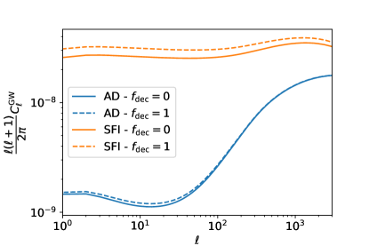
Figure 1: Plot of the angular power-spectrum of the CGWB for adiabatic (blue) and single-field inflation (orange) initial conditions, with $n_{\rm gwb}=0.35$, in the case in which all the relativistic particles at $\eta_{\rm in}$ are coupled (solid) and decoupled (dashed).

Enhancement of the angular power-spectrum

The comparison between the computation of the overdensity of the CGWB in terms of the distribution function and the results found from the energy-momentum tensor, Eq. (11), makes it possible to get the initial condition for the anisotropies of the graviton distribution,

$$\begin{split}\Gamma(\eta_{\rm in},\vec{k},\vec{q})&=\frac{1}{4-n_{\rm gwb}(q)}\left[-2\Phi(\eta_{\rm in},\vec{k})+4\Psi(\eta_{\rm in},\vec{k})\right.\\ &\left.\hskip 70.0001pt+2H(\eta_{\rm in},\vec{k})\left(1-\mu^{2}\right)\right]\,,\end{split}$$ (12)

where $\mu=\hat{k}\cdot\hat{q}$ and we have considered the expansion for an unpolarized background $H_{ij}(\eta,\vec{k})=\sum_{\lambda}H(\eta,\vec{k})e^{\lambda}_{ij}(\hat{k})$. The initial inhomogeneity contains a monopole contribution from the scalar and the tensor perturbations and a quadrupole contribution induced by only $H_{ij}$. The primordial dipole of the GWs does not contribute since the Brill-Hartle average of the velocity of the CGWB is negligible. The quadrupole term, sourced only by the large-scale tensor perturbations at the initial time, is a new term that has no analogue in the CMB case. Although it is comparatively small w.r.t. the monopole, it could play a non-negligible role, depending on the sensitivity of future GW detectors. From now on, for simplicity, we consider CGWB produced by quantum fluctuations of the metric in the case of single-field inflation or any inflationary mechanism that gives rise to adiabatic initial conditions for radiation and matter perturbations. By expanding the field in spherical harmonics we see that the initial contribution is

$$\begin{split}\Gamma_{\ell m,I}=&4\pi(-i)^{\ell}\\ &\int\frac{d^{3}k}{(2\pi)^{3}}\Bigl{[}Y^{*}_{\ell m}(\hat{k})\mathcal{R}(\vec{k})\Delta^{I-S}_{\ell}(\eta_{0},k,\eta_{\rm in})\\ &\hskip 40.00006pt+\sum_{\lambda}Y^{*\,-\lambda}_{\ell m}(\hat{k})H_{\lambda}(\vec{k})\Delta^{I-T}_{\ell}(\eta_{0},k,\eta_{\rm in})\Bigl{]}\,,\end{split}$$ (13)

where $\mathcal{R}$ is the gauge-invariant primordial curvature perturbation, $\Delta^{I-S}_{\ell}$ and $\Delta^{I-T}_{\ell}$ are the source functions given by

$$\begin{split}\Delta^{I-S}_{\ell}=&\frac{1}{4-n_{\rm gwb}(q)}\left[-2T_{\Phi}(\eta_{\rm in},k)+4T_{\Psi}(\eta_{\rm in},k)\right]\\ &\,j_{\ell}[k(\eta_{0}-\eta_{\rm in})]\,,\\ \Delta^{I-T}_{\ell}=&-\frac{1}{4-n_{\rm gwb}(q)}T_{H}(\eta_{\rm in},k)\\ &\,\frac{1}{2}\sqrt{\frac{(\ell+2)!}{(\ell-2)!}}\frac{j_{\ell}[k(\eta_{0}-\eta_{\rm in})]}{k^{2}(\eta_{0}-\eta_{\rm in})^{2}}\,.\end{split}$$ (14)

The transfer functions $T_{\Phi}$, $T_{\Psi}$, $T_{H}$ describe the time evolution of the metric perturbations, while the primordial information is contained in $\mathcal{R}$ and $H_{\lambda}$ (see Bartolo et al. (2019, 2020); Schulze et al. (2023) for more details). The angular power-spectrum of the CGWB is defined by $\langle\delta_{{\rm GW},\ell m}\delta^{*}_{{\rm GW},\ell^{\prime}m^{\prime}}\rangle=\delta_{\ell\ell^{\prime}}\delta_{mm^{\prime}}C^{\rm GW}_{\ell}$ and it is the sum of a contribution given by the initial conditions and a contribution given by the propagation through the scalar and tensor perturbations,

$$\begin{split}\frac{C^{\rm GW}_{\ell}}{4\pi(4-n_{\rm gwb})^{2}}=\int\frac{dk}{k}\Bigl{[}&P_{\mathcal{R}}(k)\left(\Delta^{I-S}_{\ell}+\Delta_{\ell}^{\rm SW}+\Delta_{\ell}^{\rm ISW}\right)^{2}\\ &+P_{T}(k)\left(\Delta^{I-T}_{\ell}+\Delta_{\ell}^{{\rm ISW}-T}\right)^{2}\Bigl{]}\,,\end{split}$$ (15)

where $P_{\mathcal{R}}(k)$ and $P_{T}(k)$ are the primordial scalar and tensor spectra respectively. Neglecting the tensor perturbations, we can see that the contribution to the anisotropy of the CGWB from the initial conditions in the case of single-field inflation enhances the angular power-spectrum w.r.t adiabatic case by a factor

$$\begin{split}\frac{C_{\ell}^{\rm SFI+SW}}{C_{\ell}^{\rm AD+SW}}&\approx\left(\frac{4T_{\Psi}+[2-n_{\rm gwb}(q)]T_{\Phi}}{-2T_{\Phi}}\right)^{2}\,.\end{split}$$ (16)

One can easily notice that when $n_{\rm gwb}=0$, the angular power-spectrum is enhanced by a factor 10. Since the total angular power-spectrum is the sum of the initial condition, SW and ISW and of the cross-correlation between these terms, differences in the initial conditions could change the way in which these three effects combine together, modifying also the scaling of the angular power-spectrum. For instance, the adiabatic initial condition has the same sign of the early-ISW, thus it sums coherently at large $\ell$, generating a bump in the spectrum, while for the initial conditions in single-field inflation they have opposite sign, thus the spectrum remains almost constant when $\ell$ increases. Additionally, it is worth noting that the angular power-spectrum of the CGWB at large angular scales is sensitive to the fractional energy density of relativistic and decoupled species Valbusa Dall’Armi et al. (2021) and to the equation of state of the Universe Malhotra et al. (2023) at early times. The impact of these parameters depends on the choice of the initial conditions. For instance, when the initial conditions are adiabatic, the angular power-spectrum is not sensitive to them when $n_{\rm gwb}\rightarrow 0$ Schulze et al. (2023). In the case of the initial conditions of single-field inflation, it is possible to show that the sensitivity to these extra parameters increases considerably. In Fig. 1 we have plotted the angular power-spectrum of the CGWB with initial conditions in the case of single-field inflation and for the standard adiabatic case, for $n_{\rm gwb}=0.35$. We have depicted the two cases in which all relativistic particles are coupled, $f_{\rm dec}=0$, and decoupled, $f_{\rm dec}=1$, showing that for the case of single-field inflation, the sensitivity to this extra parameter is larger. Moreover, it is important to note that this enhanced sensitivity of the CGWB angular power-spectrum to the fractional energy density of relativistic and decoupled species extends to both the initial conditions of single-field inflation and the equation of state parameter of the Universe at $\eta_{\rm in}$, as introduced in Malhotra et al. (2023).

Correlation between the CGWB and the CMB

At low multipoles, the angular power-spectrum of the CGWB and of the CMB are dominated by the combination of the initial condition and the SW, which is the same for both signals, since at large angular scales the two signals experience the redshift from highly-correlated metric perturbations Ricciardone et al. (2021). The constraints on the angular power-spectrum of CMB anisotropies show that the initial condition for photons is adiabatic Akrami et al. (2020), therefore, when we consider adiabatic initial conditions of the CGWB, the correlation is very large. On the other hand, the initial conditions in the case of single-field inflation are still correlated with large-scale CMB anisotropies at last-scattering, because the scalar perturbations that generate them arise from the same seeds, but since the initial conditions combine differently with the other contributions to the angular power-spectrum, the correlation decreases by a small fraction. If we define the correlation parameter as $r_{\ell}^{\rm CMB\times GW}\equiv C_{\ell}^{\rm CMB\times GW}/\sqrt{C_{\ell}^{\rm CMB}C_{\ell}^{\rm GW}}$ it is possible to show that, on large scales, in the case of adiabatic initial conditions we get $r\approx 0.98$, while in the case of single-field inflation we find $r\approx 0.8-0.9$. So, measuring such a correlation would be a way to test the nature of the initial conditions, as soon as a CGWB is detected.

Conclusions

The non-thermal nature of the cosmological background of GWs challenges the definition of the initial conditions for the overdensity of gravitons, which determines the initial contribution to CGWB anisotropies. The CGWB’s initial anisotropy strongly relies on the specific mechanism of GW production. In this letter, we have shown that the initial conditions for the cosmological background, generated by quantum fluctuations of the metric during inflation, even in the single-field case depart from the adiabaticity. Consequently, this leads to an amplification of the total CGWB angular power-spectrum when compared to the standard adiabatic case. This enhancement could play a crucial role in the detection of the anisotropies of the cosmological background in presence of intrinsic and instrumental noise Mentasti et al. (2023b, a). The inclusion of non-adiabatic initial conditions also substantially augments the sensitivity of the anisotropies to the presence of extra relativistic degrees of freedom in the early Universe, and most probably also to other early universe fundamental observables (e.g., non-Gaussianity Perna et al. (2023)). The impact of these initial conditions on the angular power-spectrum of the CGWB offers a unique means of distinguishing among different sources of GWs in the early Universe. Moreover, our result is quite general, and also applies to perturbations induced by other decoupled particle species that fluctuate during inflation. We plan to explore this effect in future work.

References

- Agazie et al. (2023a) G. Agazie et al. (NANOGrav), Astrophys. J. Lett. 951, L8 (2023a), arXiv:2306.16213 [astro-ph.HE] .
- Antoniadis et al. (2023a) J. Antoniadis et al., (2023a), arXiv:2306.16214 [astro-ph.HE] .
- Reardon et al. (2023) D. J. Reardon et al., Astrophys. J. Lett. 951, L6 (2023), arXiv:2306.16215 [astro-ph.HE] .
- Xu et al. (2023) H. Xu et al., Res. Astron. Astrophys. 23, 075024 (2023), arXiv:2306.16216 [astro-ph.HE] .
- Afzal et al. (2023) A. Afzal et al. (NANOGrav), Astrophys. J. Lett. 951, L11 (2023), arXiv:2306.16219 [astro-ph.HE] .
- Agazie et al. (2023b) G. Agazie et al. (NANOGrav), (2023b), arXiv:2306.16220 [astro-ph.HE] .
- Antoniadis et al. (2023b) J. Antoniadis et al., (2023b), arXiv:2306.16227 [astro-ph.CO] .
- Franciolini et al. (2023a) G. Franciolini, A. Iovino, Junior., V. Vaskonen, and H. Veermae, (2023a), arXiv:2306.17149 [astro-ph.CO] .
- Ellis et al. (2023) J. Ellis, M. Lewicki, C. Lin, and V. Vaskonen, (2023), arXiv:2306.17147 [astro-ph.CO] .
- Franciolini et al. (2023b) G. Franciolini, D. Racco, and F. Rompineve, (2023b), arXiv:2306.17136 [astro-ph.CO] .
- Vagnozzi (2023) S. Vagnozzi, (2023), arXiv:2306.16912 [astro-ph.CO] .
- Figueroa et al. (2023) D. G. Figueroa, M. Pieroni, A. Ricciardone, and P. Simakachorn, (2023), arXiv:2307.02399 [astro-ph.CO] .
- Liu et al. (2023) L. Liu, Z.-C. Chen, and Q.-G. Huang, (2023), arXiv:2307.01102 [astro-ph.CO] .
- Abbott et al. (2019) B. P. Abbott et al. (LIGO Scientific, Virgo), Phys. Rev. D 100, 061101 (2019), arXiv:1903.02886 [gr-qc] .
- Amaro-Seoane et al. (2017) P. Amaro-Seoane et al. (LISA), (2017), arXiv:1702.00786 [astro-ph.IM] .
- Orlando et al. (2021) G. Orlando, M. Pieroni, and A. Ricciardone, JCAP 03, 069 (2021), arXiv:2011.07059 [astro-ph.CO] .
- Corbin and Cornish (2006) V. Corbin and N. J. Cornish, Class. Quant. Grav. 23, 2435 (2006), arXiv:gr-qc/0512039 .
- Kawamura et al. (2011) S. Kawamura et al., Class. Quant. Grav. 28, 094011 (2011).
- Punturo et al. (2010) M. Punturo et al., Class. Quant. Grav. 27, 194002 (2010).
- Maggiore et al. (2020) M. Maggiore et al., JCAP 03, 050 (2020), arXiv:1912.02622 [astro-ph.CO] .
- Branchesi et al. (2023) M. Branchesi et al., (2023), arXiv:2303.15923 [gr-qc] .
- Reitze et al. (2019) D. Reitze et al., Bull. Am. Astron. Soc. 51, 035 (2019), arXiv:1907.04833 [astro-ph.IM] .
- Abbott et al. (2017) B. P. Abbott et al. (LIGO Scientific), Class. Quant. Grav. 34, 044001 (2017), arXiv:1607.08697 [astro-ph.IM] .
- Guzzetti et al. (2016) M. C. Guzzetti, N. Bartolo, M. Liguori, and S. Matarrese, Riv. Nuovo Cim. 39, 399 (2016), arXiv:1605.01615 [astro-ph.CO] .
- Bartolo et al. (2016) N. Bartolo et al., JCAP 12, 026 (2016), arXiv:1610.06481 [astro-ph.CO] .
- Caprini and Figueroa (2018) C. Caprini and D. G. Figueroa, Class. Quant. Grav. 35, 163001 (2018), arXiv:1801.04268 [astro-ph.CO] .
- Caprini et al. (2019) C. Caprini, D. G. Figueroa, R. Flauger, G. Nardini, M. Peloso, M. Pieroni, A. Ricciardone, and G. Tasinato, JCAP 11, 017 (2019), arXiv:1906.09244 [astro-ph.CO] .
- Flauger et al. (2021) R. Flauger, N. Karnesis, G. Nardini, M. Pieroni, A. Ricciardone, and J. Torrado, JCAP 01, 059 (2021), arXiv:2009.11845 [astro-ph.CO] .
- Alba and Maldacena (2016) V. Alba and J. Maldacena, JHEP 03, 115 (2016), arXiv:1512.01531 [hep-th] .
- Contaldi (2017) C. R. Contaldi, Phys. Lett. B 771, 9 (2017), arXiv:1609.08168 [astro-ph.CO] .
- Cusin et al. (2018) G. Cusin, I. Dvorkin, C. Pitrou, and J.-P. Uzan, Phys. Rev. Lett. 120, 231101 (2018), arXiv:1803.03236 [astro-ph.CO] .
- Jenkins and Sakellariadou (2018) A. C. Jenkins and M. Sakellariadou, Phys. Rev. D 98, 063509 (2018), arXiv:1802.06046 [astro-ph.CO] .
- Bertacca et al. (2020) D. Bertacca, A. Ricciardone, N. Bellomo, A. C. Jenkins, S. Matarrese, A. Raccanelli, T. Regimbau, and M. Sakellariadou, Phys. Rev. D 101, 103513 (2020), arXiv:1909.11627 [astro-ph.CO] .
- Bartolo et al. (2019) N. Bartolo, D. Bertacca, S. Matarrese, M. Peloso, A. Ricciardone, A. Riotto, and G. Tasinato, Phys. Rev. D 100, 121501 (2019), arXiv:1908.00527 [astro-ph.CO] .
- Bartolo et al. (2020) N. Bartolo, D. Bertacca, S. Matarrese, M. Peloso, A. Ricciardone, A. Riotto, and G. Tasinato, Phys. Rev. D 102, 023527 (2020), arXiv:1912.09433 [astro-ph.CO] .
- Valbusa Dall’Armi et al. (2021) L. Valbusa Dall’Armi, A. Ricciardone, N. Bartolo, D. Bertacca, and S. Matarrese, Phys. Rev. D 103, 023522 (2021), arXiv:2007.01215 [astro-ph.CO] .
- Mentasti and Peloso (2021) G. Mentasti and M. Peloso, JCAP 03, 080 (2021), arXiv:2010.00486 [astro-ph.CO] .
- Bellomo et al. (2022) N. Bellomo, D. Bertacca, A. C. Jenkins, S. Matarrese, A. Raccanelli, T. Regimbau, A. Ricciardone, and M. Sakellariadou, JCAP 06, 030 (2022), arXiv:2110.15059 [gr-qc] .
- Bartolo et al. (2022) N. Bartolo et al. (LISA Cosmology Working Group), JCAP 11, 009 (2022), arXiv:2201.08782 [astro-ph.CO] .
- Valbusa Dall’Armi et al. (2022) L. Valbusa Dall’Armi, A. Ricciardone, and D. Bertacca, JCAP 11, 040 (2022), arXiv:2206.02747 [astro-ph.CO] .
- Mentasti et al. (2023a) G. Mentasti, C. Contaldi, and M. Peloso, (2023a), arXiv:2304.06640 [gr-qc] .
- Valbusa Dall’Armi et al. (2023) L. Valbusa Dall’Armi, A. Nishizawa, A. Ricciardone, and S. Matarrese, (2023), arXiv:2301.08205 [astro-ph.CO] .
- Dodelson (2003) S. Dodelson, Modern Cosmology (Academic Press, Amsterdam, 2003).
- Malhotra et al. (2023) A. Malhotra, E. Dimastrogiovanni, G. Domènech, M. Fasiello, and G. Tasinato, Phys. Rev. D 107, 103502 (2023), arXiv:2212.10316 [gr-qc] .
- Isaacson (1967) R. A. Isaacson, Gravitational Radiation in the Limit of High Frequency, Ph.D. thesis, Maryland U. (1967).
- Misner et al. (1973) C. W. Misner, K. S. Thorne, and J. A. Wheeler, Gravitation (W. H. Freeman, San Francisco, 1973).
- Bartolo et al. (2018) N. Bartolo, A. Hoseinpour, G. Orlando, S. Matarrese, and M. Zarei, Phys. Rev. D 98, 023518 (2018), arXiv:1804.06298 [gr-qc] .
- Sachs and Wolfe (1967) R. K. Sachs and A. M. Wolfe, Astrophys. J. 147, 73 (1967).
- White et al. (1994) M. J. White, D. Scott, and J. Silk, Ann. Rev. Astron. Astrophys. 32, 319 (1994).
- Pritchard and Kamionkowski (2005) J. R. Pritchard and M. Kamionkowski, Annals Phys. 318, 2 (2005), arXiv:astro-ph/0412581 .
- Schulze et al. (2023) F. Schulze, L. Valbusa Dall’Armi, J. Lesgourgues, A. Ricciardone, N. Bartolo, D. Bertacca, C. Fidler, and S. Matarrese, (2023), arXiv:2305.01602 [gr-qc] .
- Ricciardone et al. (2021) A. Ricciardone, L. V. Dall’Armi, N. Bartolo, D. Bertacca, M. Liguori, and S. Matarrese, Phys. Rev. Lett. 127, 271301 (2021), arXiv:2106.02591 [astro-ph.CO] .
- Aghanim et al. (2020) N. Aghanim et al. (Planck), Astron. Astrophys. 641, A6 (2020), [Erratum: Astron.Astrophys. 652, C4 (2021)], arXiv:1807.06209 [astro-ph.CO] .
- Giovannini (2019) M. Giovannini, Phys. Rev. D 100, 083531 (2019), arXiv:1908.09679 [hep-th] .
- Ford and Parker (1977a) L. H. Ford and L. Parker, Phys. Rev. D 16, 1601 (1977a).
- Ford and Parker (1977b) L. H. Ford and L. Parker, Phys. Rev. D 16, 245 (1977b).
- Landau and Lifschits (1975) L. D. Landau and E. M. Lifschits, The Classical Theory of Fields, Course of Theoretical Physics, Vol. Volume 2 (Pergamon Press, Oxford, 1975).
- Babak and Grishchuk (2000) S. V. Babak and L. P. Grishchuk, Phys. Rev. D 61, 024038 (2000), arXiv:gr-qc/9907027 .
- Akrami et al. (2020) Y. Akrami et al. (Planck), Astron. Astrophys. 641, A10 (2020), arXiv:1807.06211 [astro-ph.CO] .
- Mentasti et al. (2023b) G. Mentasti, C. R. Contaldi, and M. Peloso, (2023b), arXiv:2301.08074 [gr-qc] .
- Perna et al. (2023) G. Perna, A. Ricciardone, D. Bertacca, and S. Matarrese, (2023), arXiv:2302.08429 [astro-ph.CO] .