Metric3D: Towards Zero-shot Metric 3D Prediction from A Single Image

Abstract

Reconstructing accurate 3D scenes from images is a long-standing vision task. Due to the ill-posedness of the single-image reconstruction problem, most well-established methods are built upon multi-view geometry. State-of-the-art (SOTA) monocular metric depth estimation methods can only handle a single camera model and are unable to perform mixed-data training due to the metric ambiguity. Meanwhile, SOTA monocular methods trained on large mixed datasets achieve zero-shot generalization by learning affine-invariant depths, which cannot recover real-world metrics. In this work, we show that the key to a zero-shot single-view metric depth model lies in the combination of large-scale data training and resolving the metric ambiguity from various camera models. We propose a canonical camera space transformation module, which explicitly addresses the ambiguity problems and can be effortlessly plugged into existing monocular models. Equipped with our module, monocular models can be stably trained over $8$ million of images with thousands of camera models, resulting in zero-shot generalization to in-the-wild images with unseen camera settings.

Experiments demonstrate SOTA performance of our method on $7$ zero-shot benchmarks. Notably, our method won the championship in the 2nd Monocular Depth Estimation Challenge. Our method enables the accurate recovery of metric 3D structures on randomly collected internet images, paving the way for plausible single-image metrology. The potential benefits extend to downstream tasks, which can be significantly improved by simply plugging in our model. For example, our model relieves the scale drift issues of monocular-SLAM (Fig. LABEL:Fig:_first_page_fig.), leading to high-quality metric scale dense mapping. The code is available at https://github.com/YvanYin/Metric3D.

1 Introduction

3D reconstruction from images is the core of many computer vision applications, such as autonomous driving and robotics. Main-stream methods leverage multi-view geometry [21] to confidently recover 3D structures. However, these methods cannot be applied to a single image, making 3D reconstruction hard without a prior. State-of-the-art transferable methods, such as MiDaS [40], LeReS [69], and HDN [73], learn such a prior from a large dataset, but they can only output affine-invariant depths, i.e., which are accurate only up to an unknown offset and scale. Though monocular metric depth estimation methods [71, 4] work on a single dataset with a single camera model, they cannot generalize to unseen cameras or scenes. This work aims to address the above problems by learning a zero-shot, single view, metric depth model.

According to the predicted depth, existing methods are categorized into learning metric depth [71, 64, 4, 63], learning relative depth [57, 58, 8, 7], and learning affine-invariant depth [69, 68, 40, 39, 73]. Although the metric depth methods [71, 64, 66, 4, 63] have achieved impressive accuracy on various benchmarks, they must train and test on the dataset with the same camera intrinsics. Therefore, the training datasets of metric depth methods are often small, as it is hard to collect a large dataset covering diverse scenes using one identical camera. The consequence is that all these models are not transferable – they generalize poorly to images in the wild, not to mention the camera parameters of test images can vary too. A compromise is to learn the relative depth [8, 57], which only represents one point being further or closer to another one. The application of relative depth is very limited. Learning affine-invariant depth finds a trade-off between the above two categories of methods. With large-scale data, they decouple the metric information during training and achieve impressive robustness and generalization ability. The recent state-of-the-art LeReS [69] can recover 3D scenes in the wild, but only up to an unknown scale and shift.

This work focuses on learning a zero-shot transferable model to recover metric 3D from a single image. First, we analyze the metric ambiguity issues in monocular depth estimation and study different camera parameters in depth, including the pixel size, focal length, and sensor size. We observe that the focal length is the critical factor for accurate metric recovery. By design, LeReS [69] does not take the focal length information into account during training. As shown in Sec. 3.1, only from the image appearance, various focal lengths may cause metric ambiguity, thus they decouple the depth scale in training. To solve the problem of varying focal lengths, CamConv [15] encodes the camera model in the network, which enforces the network to implicitly understand camera models from the image appearance and then bridges the imaging size to the real-world size. However, training data contains limited images and types of cameras, which challenges data diversity and network capacity. In contrast, we propose a canonical camera transformation method in training. It is inspired by the human body reconstruction methods. To improve reconstructed shape quality on countless poses, they map all samples to a canonical pose space [37] to reduce pose variance. Similarly, we transform all training data to a canonical camera space where the processed images are coarsely regarded as captured by the same camera. To achieve such transformation, we propose two different methods. The first one tries to adjust the image appearance to simulate the canonical camera, while the other one transforms the ground-truth labels for supervision. Camera models are not encoded in the network, making our method easily applicable to existing architectures. During inference, a de-canonical transformation is employed to recover metric information. To further boost the depth accuracy, we propose a random proposal normalization loss. It is inspired by the scale-shift invariant loss [69, 40, 73], which decouples the depth scale to emphasize the single image’s distribution. However, they perform on the whole image, which inevitably squeezes the fine-grained depth difference. We propose to randomly crop several patches from images and enforce the scale-shift invariant loss [69, 40] on them. Our loss emphasizes the local geometry and distribution of the single image.

With the proposed method, we can easily scale up model training to 8 million images from 11 datasets of diverse scene types (indoor and outdoor) and camera models (tens of thousands of different cameras), leading to zero-shot transferability and a significantly improved accuracy. Our model can accurately reconstruct metric 3D from randomly collected Internet images, enabling plausible single-image metrology. Different from affine-invariant depth models, our model can also directly improve various downstream tasks. As an example (Fig. LABEL:Fig:_first_page_fig.), with the predicted metric depths from our model, we can significantly reduce the scale drift of monocular SLAM [52, 51] systems, achieving much better mapping quality with real-world metric recovery. Our model also enables large-scale 3D reconstruction [23]. The model achieves the championship in the 2nd Monocular Depth Estimation Challenge [50]. To summarize, our main contributions are:

• We propose a canonical and de-canonical camera transformation method to solve the metric depth ambiguity problems from various cameras setting. It enables the learning of strong zero-shot monocular metric depth models from large-scale datasets.

• We propose a random proposal normalization loss to effectively boost the depth accuracy;

• Our model achieves state-of-the-art performance on $7$ zero-shot benchmarks. It can perform high-quality 3D metric structure recovery in the wild and benefit several downstream tasks, such as mono-SLAM [52, 35], 3D scene reconstruction [23], and metrology [75].

2 Related Work

3D reconstruction from a single image. Reconstructing various objects from a single image has been well studied [1, 54, 56]. They can produce high-quality 3D models of cars, planes, tables, and human body [41, 42]. The main challenge is how to best recover objects’ details, how to represent them with limited memory, and how to generalize to more diverse objects. However, all these methods rely on learning priors specific to a certain object class or instance, typically from 3D supervision, and can therefore not work for full scene reconstruction. Apart from these reconstructing objects works, several works focus on scene reconstruction [61] from a single image. Saxena et al. [43] construct the scene based on the assumption that the whole scene can be segmented into several small planes. With planes’ orientation and location, the 3D structure can be represented. Recently, LeReS [69] propose to use a strong monocular depth estimation model to do scene reconstruction. However, they can only recover the shape up to a scale. Zhang et al. [74] recently propose a zero-shot geometry-preserving depth estimation model that is capable of making depth predictions up to an unknown scale, without requiring scale-invariant depth annotations for training. In contrast to these works, our method can recover the metric 3D structure.

Supervised monocular depth estimation. After several benchmarks [47, 17] are established, neural network based methods [71, 66, 4] have dominated since then. Several approaches regress the continuous depth from the aggregation of information in an image [14]. As depth distribution corresponding to different RGBs can vary to a large extent, some methods [66, 4] discretize the depth and formulate this problem to a classification [64], which often achieves better performance. The generalization issue of deep models for 3D metric recovery is related to two problems. The first one is to generalize to diverse scenes, while the other one is how to predict accurate metric information under various camera settings. The first problem has been well addressed by recent methods. Some works [58, 57, 64] propose to construct a large-scale relative depth dataset, such as DIW [7] and OASIS [8], and then they target learning the relative relations. However, the relative depth loses geometric structure information. To improve the recovered geometry quality, learning affine-invariant depth methods, such as MiDaS [40], LeReS [69], and HDN [73] are proposed. By mixing large-scale data, state-of-the-art performance and the generalization over scenes are improved continuously. Note that by design, these methods are unable to recover the metric information. How to achieve both strong generalization and accurate metric information over diverse scenes is the key problem that we attempt to tackle.

Large-scale data training. Recently, various natural language problems and computer vision problems [65, 38, 29] have achieved impressive progress with large-scale data training. CLIP [38] is a promising classification model, which is trained on billions of paired image and language descriptions data. It achieved state-of-the-art performance over several classification benchmarks by zero-shot testing. For depth prediction, large-scale data training has been widely applied. Ranft et al. [40] mixed over 2 million data in training, LeReS [68] collected over $300$ thousands data, Eftekhar et al. [13] also merged millions of data to build a strong depth prediction model.

3 Method

Figure 1: Pipeline. Given an input image $I$, we first transform it to the canonical space using CSTM. The transformed image $I_{c}$ is fed into a standard depth estimation model to produce the predicted metric depth $D_{c}$ in the canonical space. During training, $D_{c}$ is supervised by a GT depth $D^{*}_{c}$ which is also transformed into the canonical space. In inference, after producing the metric depth $D_{c}$ in the canonical space, we perform a de-canonical transformation to convert it back to the space of the original input $I$. The canonical space transformation and de-canonical transformation are executed using camera intrinsics.

Preliminaries. We consider the pin-hole camera model with intrinsic parameters are: [[$\nicefrac{{\hat{f}}}{{\delta}},0,u_{0}$], [$0,\nicefrac{{\hat{f}}}{{\delta}},v_{0}$], [$0,0,1$]], where $\hat{f}$ is the focal length (in micrometers), $\delta$ is the pixel size (in micrometers), and $(u_{0},v_{0})$ is the principle center. $f=\nicefrac{{\hat{f}}}{{\delta}}$ is the pixel-represented focal length used in vision algorithms.

3.1 Metric Ambiguity Analysis

Fig. 2 presents an example of photos taken by different cameras and at different distances. Only from the image’s appearance, one may think the last two photos are taken at a similar location by the same camera. In fact, due to different focal lengths, these are captured at different locations. Thus, camera intrinsic parameters are critically important for the metric estimation from a single image, as otherwise, the problem is ill posed. To avoid such metric ambiguity, recent methods, such as MiDaS [40] and LeReS [69], decouple the metric from the supervision and compromise learning the affine-invariant depth.

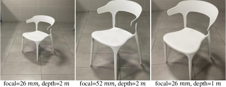
Figure 2: Photos of a chair captured at different distances with different cameras. The first two photos are captured at the same distance but with different cameras, while the last one is taken at a closer distance with the same camera as the first one.

Fig. 3 (A) shows a simple pin-hole perspective projection. Object $A$ locating at $d_{a}$ is projected to $A^{\prime}$. Based on the principle of similarity, we have the equation:

$$\vspace{-1em}d_{a}=\hat{S}\Bigl{[}\frac{\hat{f}}{\hat{S^{\prime}}}\Bigr{]}=\hat{S}\cdot\alpha$$ (1)

where $\hat{S}$ and $\hat{S^{\prime}}$ are the real and imaging size respectively. $\hat{\cdot}$ denotes variables are in the physical metric (e.g., millimeter). To recover $d_{a}$ from a single image, focal length, imaging size of the object, and real-world object size must be available. Estimating the focal length from a single image is a challenging and ill-posed problem. Although several methods [69, 22] have explored, the accuracy is still far from being satisfactory. Here, we simplify the problem by assuming the focal length of a training/test image is available. In contrast, understanding the imaging size is much easier for a neural network. To obtain the real-world object size, a neural network needs to understand the semantic scene layout and the object, at which a neural network excels. We define $\alpha=\nicefrac{{\hat{f}}}{{\hat{S^{\prime}}}}$, so $d_{a}$ is proportional to $\alpha$.

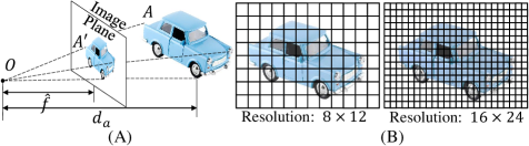
Figure 3: Pinhole camera model. (A) Object $A$ at the distance $d_{a}$ is projected to the image plane. (B) Using two cameras to capture the car. The left one has a larger pixel size. Although the projected imaging sizes are the same, the pixel-represented images (resolution) are different.

We make the following observations regarding sensor size, pixel size, and focal length.

O1: Sensor size and pixel size do not affect the metric depth estimation. Based on the perspective projection (Fig. 3 (A)), the sensor size only affects the field of view (FOV) and is irrelevant to $\alpha$, thus does not affect the metric depth estimation. For the pixel size, we assume two cameras with different pixel sizes ($\delta_{1}=2\delta_{2}$) but the same focal length $\hat{f}$ to capture the same object locating at $d_{a}$. Fig. 3 (B) shows their captured photos. According to the preliminaries, the pixel-represented focal length $f_{1}=\frac{1}{2}f_{2}$. As the second camera has a smaller pixel size, although in the same projected imaging size $\hat{S^{\prime}}$, the pixel-represented image resolution is $S^{\prime}_{1}=\frac{1}{2}S^{\prime}_{2}$. According to Eq. (1), $\frac{\hat{f}}{\delta_{1}\cdot S^{\prime}_{1}}=\frac{\hat{f}}{\delta_{2}\cdot S^{\prime}_{2}}$, i.e. $\alpha_{1}=\alpha_{2}$, so $d_{1}=d_{2}$. Therefore, different camera sensors would not affect the metric depth estimation.

O2: The focal length is vital for metric depth estimation. Fig. 2 shows the metric ambiguity issue caused by the unknown focal length. Fig. 4 illustrates this. If two cameras ($\hat{f}_{1}=2\hat{f}_{2}$) are at distances $d_{1}=2d_{2}$, the imaging sizes on cameras are the same. Thus, only from the appearance, the network will be confused when supervised with different labels. Based on this observation, we propose a canonical camera transformation method to solve the supervision and image appearance conflicts.

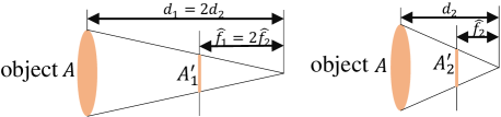
Figure 4: Illustration of two cameras with different focal length at different distance. As $f_{1}=2f_{2}$ and $d_{1}=2d_{2}$, $A$ is projected to two image planes with the same imaging size (i.e. $A^{{}^{\prime}}_{1}=A^{{}^{\prime}}_{2}$).

3.2 Canonical Camera Transformation

The core idea is to set up a canonical camera space ($(f_{x}^{c},f_{y}^{c})$, $f_{x}^{c}=f_{y}^{c}=f^{c}$ in experiments) and transform all training data to this space. Consequently, all data can roughly be regarded as captured by the canonical camera. We propose two transformation methods, i.e. either transforming the input image ($\mathbf{I}\in\mathbb{R}^{H\times W\times 3}$) or the ground-truth (GT) label ($\mathbf{D}\in\mathbb{R}^{H\times W}$). The original intrinsics are $\{f,u_{0},v_{0}\}$.

Method1: transforming depth labels (CSTM_label). Fig. 2’s ambiguity is for depths. Thus our first method directly transforms the ground-truth depth labels to solve this problem. Specifically, we scale the ground-truth depth ($\mathbf{D}^{*}$) with the ratio $\omega_{d}=\frac{f^{c}}{f}$ in training, i.e., $\mathbf{D}^{*}_{c}=\omega_{d}\mathbf{D}^{*}$. The original camera model is transformed to $\{f^{c},u_{0},v_{0}\}$. In inference, the predicted depth ($\mathbf{D}_{c}$) is in the canonical space and needs to perform a de-canonical transformation to recover the metric information, i.e., $\mathbf{D}=\frac{1}{\omega_{d}}\mathbf{D}_{c}$. Note the input $\mathbf{I}$ does not perform any transformation, i.e., $\mathbf{I}_{c}=\mathbf{I}$.

Method2: transforming input images (CSTM_image). From another view, the ambiguity is caused by the similar image appearance. Thus this method is to transform the input image to simulate the canonical camera imaging effect. Specifically, the image $\mathbf{I}$ is resized with the ratio $\omega_{r}=\frac{f^{c}}{f}$, i.e., $\mathbf{I}_{c}=\mathcal{T}(\mathbf{I},\omega_{r})$, where $\mathcal{T}(\cdot)$ denotes image resize. The optical center is resized, thus the canonical camera model is $\{f^{c},\omega_{r}u_{0},\omega_{r}v_{0}\}$. The ground-truth labels are resized without any scaling, i.e., $\mathbf{D}^{*}_{c}=\mathcal{T}(\mathbf{D}^{*},\omega_{r})$. In inference, the de-canonical transformation is to resize the prediction to the original size without scaling, i.e., $\mathbf{D}=\mathcal{T}(\mathbf{D}_{c},\frac{1}{\omega_{r}})$.

Fig. 1 shows the pipeline. After performing either transformation, we randomly crop a patch for training. The cropping only adjusts the FOV and the optical center, thus not causing any metric ambiguity issues. In the labels transformation method $\omega_{r}=1$ and $\omega_{d}=\frac{f^{c}}{f}$, while $\omega_{d}=1$ and $\omega_{r}=\frac{f^{c}}{f}$ in the images transformation method. The training objective is as follows:

$$\min_{\theta}\left|\mathcal{N}_{d}(\mathbf{I}_{c},\theta)-\mathbf{D}^{*}_{c}\right|\vspace{-0.5 em}$$ (2)

where $\theta$ is the network’s ($\mathcal{N}_{d}(\cdot)$) parameters, $\mathbf{D}^{*}_{c}$ and $\mathbf{I}_{c}$ are transformed ground-truth depth labels and images.

Mix-data training is an effective way to boost generalization. We collect $11$ datasets for training, see the supplementary materials for details. In the mixed data, over 10K different cameras are included. All collected training data have included paired camera intrinsic parameters, which are used in our canonical transformation module.

Supervision. To further boost the performance, we propose a random proposal normalization loss (RPNL). The scale-shift invariant loss [40, 69] is widely applied for the affine-invariant depth estimation, which decouples the depth scale to emphasize the single image distribution. However, such normalization based on the whole image inevitably squeezes the fine-grained depth difference, particularly in close regions. Inspired by this, we propose to randomly crop several patches ($p_{i(i=0,...,M)}\in\mathbb{R}^{h_{i}\times w_{i}}$) from the ground truth $\mathbf{D}^{*}_{c}$ and the predicted depth $\mathbf{D}_{c}$. Then we employ the median absolute deviation normalization [48] for paired patches. By normalizing the local statistics, we can enhance local contrast. The loss function is as follows:

$$L_{{\rm RPNL}}=\frac{1}{MN}\sum_{p_{i}}^{M}\sum_{j}^{N}\lvert\frac{d^{*}_{p_{i},j}-\mu(d^{*}_{p_{i},j})}{\frac{1}{N}\sum_{j}^{N}\left|d^{*}_{p_{i},j}-\mu(d^{*}_{p_{i},j})\right|}-$$

$$\frac{d_{p_{i},j}-\mu(d_{p_{i},j})}{\frac{1}{N}\sum_{j}^{N}\left|d_{p_{i},j}-\mu(d_{p_{i},j})\right|}\rvert$$ (3)

where $d^{*}\in\mathbf{D}^{*}_{c}$ and $d\in\mathbf{D}_{c}$ are the ground truth and predicted depth respectively. $\mu(\cdot)$ and is the median of depth. $M$ is the number of proposal crops, which is set to 32. During training, proposals are randomly cropped from the image by $0.125$ to $0.5$ of the original size. Furthermore, several other losses are employed, including the scale-invariant logarithmic loss [14] $L_{silog}$, pair-wise normal regression loss [69]$L_{{\rm PWN}}$, virtual normal loss [64] $L_{{\rm VNL}}$. Note $L_{silog}$ is a variant of L1 loss. The overall losses are as follows.

$$L=L_{{\rm PWN}}+L_{{\rm VNL}}+L_{silog}+L_{{\rm RPNL}}.$$

4 Experiments

Dataset details. We collect $11$ public RGB-D datasets, and over $8$ million data for training. It spreads over diverse indoor and outdoor scenes. Note that all datasets have provided camera intrinsic parameters. Apart from the test split of training datasets, we collect $7$ unseen datasets for robustness and generalization evaluation. Details of employed data are reported in the supplementary materials.

Implementation details. We employ an UNet architecture with the ConvNext-large [33] backbone. ImageNet-22K pre-trained weights are used for initialization. We use AdamW with a batch size of $192$, an initial learning rate $0.0001$ for all layers, and the polynomial decaying method with the power of $0.9$. We train our final model on $48$ A100 GPUs for $500$K iterations. Following the DiverseDepth [64], we balance all datasets in a mini-batch to ensure each dataset accounts for an almost equal ratio. During training, images are processed by the canonical camera transformation module, flipped horizontally with a $50\%$ chance, and then randomly cropped into $512\times 960$ pixels. For the ablation experiments, training settings are different as we sample $5000$ images from each dataset for training. We trained on $8$ GPUs for $150$K iterations.

Evaluation details. a) To show the robustness of our metric depth estimation method, we test on 8 zero-shot benchmarks, including NYUv2 [47], KITTI [17], NuScenes [6], 7-scenes [46], iBIMS-1 [26], DIODE [53], ETH3D [45]. Following previous works [71], absolute relative error (AbsRel), the accuracy under threshold ($\delta_{i}<1.25^{i},i=1,2,3$), root mean squared error (RMS), root mean squared error in log space (RMS_log), and log10 error (log10) metrics are employed. b) Furthermore, we also follow current affine-invariant depth benchmarks [69, 73] (Tab. 4) to evaluate the generalization ability on $5$ zero-shot datasets, i.e., NYUv2, DIODE, ETH3D, ScanNet [11], and KITTI. We mainly compare with large-scale data trained models. Note that in this benchmark we follow existing methods to apply the scale shift alignment before evaluation. c) To evaluate our metric 3D reconstruction quality, we randomly sample 9 unseen scenes from NYUv2 and use colmap [44] to obtain the camera poses for multi-frame reconstruction. Chamfer $l_{1}$ distance and the F-score [25] are used to evaluate the reconstruction accuracy. d) In dense-SLAM experiments, following Li et al. [31], we test on the KITTI odometry benchmark [17] and evaluate the average translational RMS drift ($\%,t_{rel}$) and rotational RMS drift ($\degree/100m,r_{rel}$) errors [17]. Note that all these depth and reconstruction evaluations use the same trained model.

4.1 Zero-shot Generalization Test

Table 1: Quantitative comparison on NYUv2 and KITTI benchmarks. Both datasets are unseen to our model, but we can achieve comparable performance with state-of-the-art methods.

NYUv2 Benchmark
Method	$\boldsymbol{\delta_{1}}$$\uparrow$	$\boldsymbol{\delta_{2}}$$\uparrow$	$\boldsymbol{\delta_{3}}$$\uparrow$	AbsRel$\downarrow$	log10$\downarrow$	RMS$\downarrow$
Li et al. [30]	$0.788$	$0.958$	$0.991$	$0.143$	$0.063$	$0.635$
Laina et al. [28]	$0.811$	$0.953$	$0.988$	$0.127$	$0.055$	$0.573$
VNL  [66]	$0.875$	$0.976$	$0.994$	$0.108$	$0.048$	$0.416$
TrDepth [63]	$0.900$	$0.983$	$0.996$	$0.106$	$0.045$	$0.365$
Adabins [4]	$0.903$	${0.984}$	$\underline{0.997}$	$0.103$	$0.044$	$0.364$
NeWCRFs [71]	${0.922}$	$\boldsymbol{0.992}$	$\boldsymbol{0.998}$	$0.095$	$0.041$	$\underline{0.334}$
Ours CSTM_image	$\boldsymbol{0.925}$	$0.983$	$0.994$	$\underline{0.092}$	$\underline{0.040}$	${0.341}$
Ours CSTM_label	$\underline{0.944}$	$\underline{0.986}$	$0.995$	$\boldsymbol{0.083}$	$\boldsymbol{0.035}$	$\boldsymbol{0.310}$
KITTI Benchmark
Method	$\boldsymbol{\delta_{1}}$$\uparrow$	$\boldsymbol{\delta_{2}}$$\uparrow$	$\boldsymbol{\delta_{3}}$$\uparrow$	AbsRel $\downarrow$	RMS $\downarrow$	RMS_log $\downarrow$
Guo et al. [20]	$0.902$	$0.969$	$0.986$	$0.090$	$3.258$	$0.168$
VNL [66]	${0.938}$	${0.990}$	${0.998}$	${0.072}$	$3.258$	${0.117}$
TrDepth [63]	$0.956$	$0.994$	$0.999$	$0.064$	$2.755$	$0.098$
Adabins [4]	$0.964$	$0.995$	$0.999$	$\underline{0.058}$	$2.360$	$0.088$
NeWCRFs [71]	$\boldsymbol{0.974}$	$\boldsymbol{0.997}$	$\underline{0.999}$	$\boldsymbol{0.052}$	$\boldsymbol{2.129}$	$\boldsymbol{0.079}$
Ours CSTM_image	$\underline{0.967}$	$\underline{0.995}$	$\boldsymbol{0.999}$	$0.060$	${2.843}$	$\underline{0.087}$
Ours CSTM_label	${0.964}$	${0.993}$	${0.998}$	$0.058$	${2.770}$	${0.092}$

Table 2: Quantitative comparison of 3D scene reconstruction with LeReS [69], DPT [39], RCVD [27], SC-DepthV2 [5], and a learning-based MVS method (DPSNet [23]) on 9 unseen NYUv2 scenes. Apart from DPSNet and ours, other methods have to align the scale with ground truth depth for each frame. As a result, our reconstructed 3D scenes achieve the best performance.

Method	Basement_0001a		Bedroom_0015		Dining_room_0004		Kitchen_0008		Classroom_0004		Playroom_0002		Office_0024		Office_0004		Dining_room_0033
	C-$l_{1}$$\downarrow$	F-score $\uparrow$	C-$l_{1}$$\downarrow$	F-score $\uparrow$	C-$l_{1}$$\downarrow$	F-score $\uparrow$	C-$l_{1}$$\downarrow$	F-score $\uparrow$	C-$l_{1}$$\downarrow$	F-score $\uparrow$	C-$l_{1}$$\downarrow$	F-score $\uparrow$	C-$l_{1}$$\downarrow$	F-score $\uparrow$	C-$l_{1}$$\downarrow$	F-score $\uparrow$	C-$l_{1}$$\downarrow$	F-score $\uparrow$
RCVD [27]	0.364	0.276	0.074	0.582	0.462	0.251	0.053	0.620	0.187	0.327	0.791	0.187	0.324	0.241	0.646	0.217	0.445	0.253
SC-DepthV2 [5]	0.254	0.275	0.064	0.547	0.749	0.229	0.049	0.624	0.167	0.267	0.426	0.263	0.482	0.138	0.516	0.244	0.356	0.247
DPSNet [23]	0.243	0.299	0.195	0.276	0.995	0.186	0.269	0.203	0.296	0.195	0.141	0.485	0.199	0.362	0.210	0.462	0.222	0.493
DPT [69]	0.698	0.251	0.289	0.226	0.396	0.364	0.126	0.388	0.780	0.193	0.605	0.269	0.454	0.245	0.364	0.279	0.751	0.185
LeReS [69]	0.081	0.555	0.064	0.616	0.278	0.427	0.147	0.289	0.143	0.480	0.145	0.503	0.408	0.176	0.096	0.497	0.241	0.325
Ours	0.042	0.736	0.059	0.610	0.159	0.485	0.050	0.645	0.145	0.445	0.036	0.814	0.069	0.638	0.045	0.700	0.060	0.663

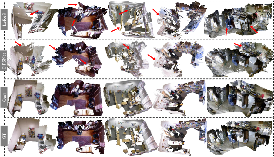
Figure 5: Reconstruction of zero-shot scenes with multiple views. We sample several NYUv2 scenes for 3D reconstruction comparison. As our method can predict accurate metric depth, thus all frame’s predictions are fused together for scene reconstruction. By contrast, LeReS [69]’s depth is up to an unknown scale and shift, which causes noticeable distortions. DPSNet [23] is a multi-view stereo method, which cannot work well on low-texture regions.

Evaluation on metric depth benchmarks. To evaluate the accuracy of predicted metric depth, firstly, we compare with state-of-the-art (SOTA) metric depth prediction methods on NYUv2 [47], KITTI [18]. We use the same model to do all evaluations. Results are reported in Tab. 1. Without any fine-tuning or metric adjustment, we can achieve comparable performance with SOTA methods, which are trained on benchmarks for hundreds of epochs.

Furthermore, We collect $6$ unseen datasets to do more metric accuracy evaluation. These datasets contain a wide range of indoor and outdoor scenes, including rooms, buildings, and driving scenes. The camera models are also various, e.g. 7scenes has a short focal length (around 500), while ETH3D is 2000. We mainly compare with the SOTA metric depth estimation methods and take their NYUv2 and KITTI models for indoor and outdoor scenes evaluation respectively. From Tab. 3, we observe that although 7Scenes is similar to NYUv2 and NuScenes is similar to KITTI, existing methods face a noticeable performance decrease. In contrast, our model is more robust.

Table 3: Quantitative comparison with SOTA metric depth methods on $6$ unseen benchmarks. For SOTA methods, we use their NYUv2 and KITTI models for indoor and outdoor scenes evaluation respectively, while we use the same model for all zero-shot testing.

Method	DIODE(Indoor)	iBIMS-1	7Scenes	DIODE(Outdoor)	ETH3D	NuScenes
	Indoor scenes (AbsRel$\downarrow$/RMS$\downarrow$)			Outdoor scenes (AbsRel$\downarrow$/RMS$\downarrow$)
Adabins [4]	0.443 / 1.963	0.212 / 0.901	0.218 / 0.428	0.865 / 10.35	1.271 / 6.178	0.445 / 10.658
NewCRFs [71]	0.404 / 1.867	0.206 / 0.861	0.240 / 0.451	0.854 / 9.228	0.890 / 5.011	0.400 / 12.139
Ours_CSTM_label	0.252 / 1.440	0.160 / 0.521	0.183 / 0.363	0.414 / 6.934	0.416 / 3.017	0.154 / 7.097
Ours_CSTM_image	0.268 / 1.429	0.144 / 0.646	0.189 / 0.388	0.535 / 6.507	0.342 / 2.965	0.147 / 5.889

Table 4: Comparison with SOTA affine-invariant depth methods on 5 zero-shot transfer benchmarks. Our model significantly outperforms previous methods and sets new state-of-the-art. Following the benchmark setting, all methods have manually aligned the scale and shift.

Method	Backbone	#Params	NYUv2		KITTI		DIODE		ScanNet		ETH3D		Rank
			AbsRel$\downarrow$	$\delta_{1}$$\uparrow$	AbsRel$\downarrow$	$\delta_{1}$$\uparrow$	AbsRel$\downarrow$	$\delta_{1}$$\uparrow$	AbsRel$\downarrow$	$\delta_{1}$$\uparrow$	AbsRel$\downarrow$	$\delta_{1}$$\uparrow$
DiverseDepth [64]	ResNeXt50 [60]	25M	$0.117$	$0.875$	$0.190$	$0.704$	$0.376$	$0.631$	$0.108$	$0.882$	$0.228$	$0.694$	$7.7$
MiDaS [40]	ResNeXt101	88M	$0.111$	$0.885$	$0.236$	$0.630$	$0.332$	$0.715$	$0.111$	$0.886$	$0.184$	$0.752$	$7.2$
Leres [69]	ResNeXt101		$0.090$	${0.916}$	${0.149}$	${0.784}$	${0.271}$	${0.766}$	${0.095}$	${0.912}$	${0.171}$	${0.777}$	$5.4$
Omnidata [13]	ViT-base		0.074	0.945	0.149	0.835	0.339	0.742	0.077	0.935	0.166	0.778	$4.9$
HDN [73]	ViT-Large [12]	306M	$0.069$	$0.948$	$0.115$	$0.867$	$0.246$	$0.780$	$0.080$	$0.939$	$0.121$	$0.833$	$3.7$
DPT-large [39]	ViT-Large		0.098	0.903	0.10	0.901	0.182	0.758	0.078	0.938	0.078	0.946	$3.8$
Ours CSTM_image	ConvNeXt-large [33]	198M	$\underline{0.058}$	$\underline{0.963}$	0.053	$\underline{0.965}$	$\underline{0.211}$	0.825	0.074	0.942	0.064	0.965	$1.3$
Ours CSTM_label	ConvNeXt-large		0.050	0.966	$\underline{0.058}$	0.970	$0.224$	$\underline{0.805}$	0.074	$\underline{0.941}$	$\underline{0.066}$	$\underline{0.964}$	$1.8$

Generalization over diverse scenes. Affine-invariant depth benchmarks decouple the scale’s effect, which aims to evaluate the model’s generalization ability to diverse scenes. Recent impact works, such as MiDaS, LeReS, and DPT, achieved promising performance on them. Following them, we test on 5 datasets and manually align the scale and shift to the ground-truth depth before evaluation. Results are reported in Tab. 4. Although our method enforces the network to recover more challenging metric information, our method outperforms them by a large margin on most datasets.

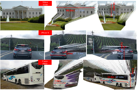
Figure 6: Reconstruction of in-the-wild scenes. We collect several Flickr photos, which are captured by various cameras. With photos’ metadata, we reconstruct the 3D metric shape and measure structures’ sizes. Red and blue marks are ours and ground-truth sizes respectively.

4.2 Applications Based on Our Method

In these experiments, we apply the CSTM_image model to various tasks.

3D scene reconstruction . To demonstrate our work can recover the 3D metric shape in the wild, we first do the quantitative comparison on 9 NYUv2 scenes, which are unseen during training. We predict the per-frame metric depth and then fuse them together with provided camera poses. Results are reported in Tab. 2. We compare with the video consistent depth prediction method (RCVD [27]), the unsupervised video depth estimation method (SC-DepthV2 [5]), the 3D scene shape recovery method (LeReS [69]), affine-invariant depth estimation method (DPT [39]), and the multi-view stereo reconstruction method (DPSNet [23]). Apart from DPSNet and our method, other methods have to align the scale with the ground truth depth for each frame. Although our method does not aim for the video or multi-view reconstruction problem, our method can achieve promising consistency between frames and reconstruct much more accurate 3D scenes than others on these zero-shot scenes. From the qualitative comparison in Fig. 5. our reconstructions have much less noise and outliers.

Dense-SLAM mapping. Monocular SLAM is an important robotics application. It only relies on a monocular video input to create the trajectory and dense 3D mapping. Owing to limited photometric and geometric constraints, existing methods face serious scale drift problems in large scenes and cannot recover the metric information. Our robust metric depth estimation method is a strong depth prior to the SLAM system. To demonstrate this benefit, we naively input our metric depth to the SOTA SLAM system, Droid-SLAM [52], and evaluate the trajectory on KITTI. We do not do any tuning on the original system. Trajectory comparisons are reported in Tab. 5. As Droid-SLAM can access accurate per-frame metric depth, like an RGB-D SLAM, the translation drift ($t_{rel}$) decreases significantly. Furthermore, with our depths, Droid-SLAM can perform denser and more accurate 3D mapping. An example is shown in Fig. LABEL:Fig:_first_page_fig. and more cases are shown in the supplementary materials.

We also test on the ETH3D SLAM benchmarks. Results are reported in Tab. 6. Droid with our depths has much better SLAM performance. As the ETH3D scenes are all small-scale indoor scenes, the performance improvement is less than that on KITTI.

Table 5: Comparison with SOTA SLAM methods on KITTI. We input predicted metric depth to the Droid-SLAM [52] (‘Droid+Ours’), which outperforms others by a large margin on trajectory accuracy.

Method	Seq 00	Seq 02	Seq 05	Seq 06	Seq 08	Seq 09	Seq 10
	Translational RMS drift ($t_{rel},\downarrow$) / Rotational RMS drift ($r_{rel},\downarrow$)
GeoNet [70]	27.6/5.72	42.24/6.14	20.12/7.67	9.28/4.34	18.59/7.85	23.94/9.81	20.73/9.1
VISO2-M [49]	12.66/2.73	9.47/1.19	15.1/3.65	6.8/1.93	14.82/2.52	3.69/1.25	21.01/3.26
ORB-V2 [36]	11.43/0.58	10.34/0.26	9.04/0.26	14.56/0.26	11.46/0.28	9.3/0.26	2.57/0.32
Droid [52]	33.9/0.29	34.88/0.27	23.4/0.27	17.2/0.26	39.6/0.31	21.7/0.23	7/0.25
Droid+Ours	1.44/0.37	2.64/0.29	1.44/0.25	0.6/0.2	2.2/0.3	1.63/0.22	2.73/0.23

Table 6: Comparison of VO error on ETH3D benchmark. Droid SLAM system is input with our depth (‘Droid + Ours’), and ground-truth depth (‘Droid + GT’). The average trajectory error is reported.

	Einstein_global	Manquin4	Motion1	Plantscene3	sfm_house_loop	sfm_lab_room2
	Average trajectory error ($\downarrow$)
Droid	4.7	0.88	0.83	0.78	5.64	0.55
Droid + Ours	1.5	0.69	0.62	0.34	4.03	0.53
Droid + GT	0.7	0.006	0.024	0.006	0.96	0.013

Metrology in the wild. To show the robustness and accuracy of our recovered metric 3D, we download Flickr photos captured by various cameras and collect coarse camera intrinsic parameters from their metadata. We use our CSTM_image model to reconstruct their metric shape and measure structures’ sizes (marked in red in Fig. 6), while the ground-truth sizes are in blue. It shows that our measured sizes are very close to the ground-truth sizes.

4.3 Ablation Study

Ablation on canonical transformation. We study the effect of our proposed canonical transformation for the input images (‘CSTM_input’) and the canonical transformation for the ground-truth labels (‘CSTM_output’). Results are reported in Tab. 7. We train the model on sampled mixed data (55K images) and test it on 6 datasets. A naive baseline (‘Ours w/o CSTM’) is to remove CSTM modules and enforce the same supervision as ours. Without CSTM, the model is unable to converge when training on mixed metric datasets and cannot achieve metric prediction ability on zero-shot datasets. This is why recent mixed-data training methods compromise learning the affine-invariant depth to avoid metric issues. In contrast, our two CSTM methods both can enable the model to achieve the metric prediction ability, and they can achieve comparable performance. Tab. 1 also shows comparable performance. Therefore, both adjusting the supervision and the input image appearance during training can solve the metric ambiguity issues. Furthermore, we compare with CamConvs [15], which encodes the camera model in the decoder with a 4-channel feature. ‘CamConvs’ employ the same training schedule, model, and training data as ours. This method enforces the network to implicitly understand various camera models from the image appearance and then bridges the imaging size to the real-world size. We believe that this method challenges the data diversity and network capacity, thus their performance is worse than ours.

Table 7: Effectiveness of our CSTM. CamConvs [15] directly encodes various camera models in the network, while we perform a simple yet effective transformation to solve the metric ambiguity. Without CSTM, the model cannot achieve transferable metric prediction ability.

Method	DDAD	Lyft	DS	NS	KITTI	NYU
	Test set of train. data (AbsRel$\downarrow$)			Zero-shot test set (AbsRel$\downarrow$)
w/o CSTM	$0.530$	$0.582$	$0.394$	$1.00$	$0.568$	$0.584$
CamConvs [15]	$0.295$	$0.315$	$0.213$	$0.423$	$0.178$	$0.333$
Ours CSTM_image	$0.190$	$0.235$	$0.182$	$0.197$	$0.097$	$0.210$
Ours CSTM_label	$0.183$	$0.221$	$0.201$	$0.213$	$0.081$	$0.212$

Ablation on canonical space. We study the effect of the canonical camera here, i.e., the canonical focal length. We train the model on the small sampled dataset and test it on the validation set of training data and testing data. The average AbsRel error is calculated. We experiment on 3 different focal lengths, i.e., 500, 1000, 1500. Experiments show that $focal=1000$ has slightly better performance than others, see Fig. 7 for details. Thus we set the canonical focal length to 1000 in our experiments.

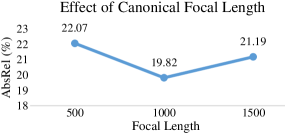
Figure 7: Effect of different canonical focal lengths. We experiment on different canonical focal lengths and find that too large or small focal lengths will impact the performance.

Effectiveness of the random proposal normalization loss. To show the effectiveness of our proposed random proposal normalization loss (RPNL), we experiment on the sampled small dataset. Results are shown in Tab. 8. We test on the DDAD, Lyft, DrivingStereo (DS), NuScenes (NS), KITTI, and NYUv2. The ‘baseline’ employs all losses except our RPNL. We compare it with ‘baseline + RPNL’ and ‘baseline + SSIL [40]’. We can observe that our proposed random proposal normalization loss can further improve the performance. In contrast, the scale-shift invariant loss [40], which does the normalization on the whole image, can only slightly improve the performance.

Table 8: Effectiveness of random proposal normalization loss. Baseline is supervised by ‘$L_{{\rm PWN}}+L_{{\rm VNL}}+L_{silog}$’. SSIL is the scale-shift invariant loss proposed in  [40].

Method	DDAD	Lyft	DS	NS	KITTI	NYUv2
	Test set of train. data (AbsRel$\downarrow$)			Zero-shot test set (AbsRel$\downarrow$)
baseline	$0.204$	$0.251$	$0.184$	$0.207$	$0.104$	$0.230$
baseline + SSIL [40]	$0.197$	$0.263$	$0.259$	$0.206$	$0.105$	$0.216$
baseline + RPNL	0.190	0.235	0.182	0.197	0.097	0.210

5 Conclusion

In this paper, we tackle the problem of reconstructing the 3D metric scene from a single monocular image. To solve the depth ambiguity in image appearance caused by various focal lengths, we propose a canonical camera space transformation method. With our method, we can easily merge millions of data captured by 10k cameras to train one metric depth model. To improve the robustness, we collected over $8$M data for training. Several zero-shot evaluations show the effectiveness and robustness of our work. We further show the ability to do metrology on randomly collected internet images and dense mapping on large-scale scenes.

6 Appendix

6.1 Datasets and Training and Testing

We collect over $8$M data from 11 public datasets for training. Datasets are listed in Tab. 9. The autonomous driving datasets, including DDAD [19], Lyft [24], DrivingStereo [62], Argoverse2 [55], DSEC [16], and Pandaset [59], have provided LiDar and camera intrinsic and extrinsic parameters. We project the LiDar to image planes to obtain ground-truth depths. In contrast, Cityscapes [10], DIML [9], and UASOL [2] only provide calibrated stereo images. We use draftstereo [32] to achieve pseudo ground-truth depths. Mapillary PSD [34] dataset provides paired RGB-D, but the depth maps are achieved from a structure-from-motion method. The camera intrinsic parameters are estimated from the SfM. We believe that such achieved metric information is noisy. Thus we do not enforce learning-metric-depth loss on this data, i.e., $L_{silog}$, to reduce the effect of noises. For the Taskonomy [72] dataset, we follow LeReS [68] to obtain the instance planes, which are employed in the pair-wise normal regression loss. During training, we employ the training strategy from [67] to balance all datasets in each training batch.

The testing data is listed in Tab. 9. All of them are captured by high-quality sensors. In testing, we employ their provided camera intrinsic parameters to perform our proposed canonical space transformation.

Table 9: Training and testing datasets used in experiments.

Datasets	Scenes	Label	Size	# Cam.
Training Data
DDAD [19]	Outdoor	LiDar	$\sim$80K	36+
Lyft [24]	Outdoor	LiDar	$\sim$50K	6+
Driving Stereo (DS) [62]	Outdoor	Stereo†	$\sim$181K	1
DIML [9]	Outdoor	Stereo†	$\sim$122K	10
Arogoverse2 [55]	Outdoor	LiDar	$\sim$3515K	6+
Cityscapes [10]	Outdoor	Stereo†	$\sim$170K	1
DSEC [16]	Outdoor	LiDar	$\sim$26K	1
Mapillary PSD [34]	Outdoor	SfM‡	750K	1000+
Pandaset [59]	Outdoor	LiDar	$\sim$48K	6
UASOL [2]	Outdoor	Stereo†	$\sim$137K	1
Taskonomy [72]	Indoor	LiDar	$\sim$4M	$\sim$1M
Testing Data
NYU [47]	Indoor	Kinect	654	1
KITTI [17]	Outdoor	LiDar	652	4
ScanNet [11]	Indoor	Kinect	700	1
NuScenes (NS) [6]	Outdoor	LiDar	10K	6
ETH3D [45]	Outdoor	LiDar	431	1
DIODE [53]	In/Out	LiDar	771	1
7Scenes [46]	Indoor	Kinect	17k	1
iBims-1 [26]	Indoor	LiDar	100	1

• ‘Stereo’: we use RaftStereo [32] to retrieve the pseudo ground truth.

• ‘SfM’: pseudo ground truth is retrieved by structure from motion.

6.2 Details for Some Experiments

Evaluation of zero-shot 3D scene reconstruction. In this experiment, we use all methods’ released models to predict each frame’s depth and use the ground-truth poses and camera intrinsic parameters to reconstruct point clouds. When evaluating the reconstructed point cloud, we employ the iterative closest point (ICP) [3] algorithm to match the predicted point clouds with ground truth by a pose transformation matrix. Finally, we evaluate the Chamfer $\ell_{1}$ distance and F-score on the point cloud.

Reconstruction of in-the-wild scenes. We collect several photos from Flickr. From their associated camera metadata, we can obtain the focal length $\hat{f}$ and the pixel size $\delta$. According to $\nicefrac{{\hat{f}}}{{\delta}}$, we can obtain the pixel-represented focal length for 3D reconstruction and achieve the metric information. We use meshlab software to measure some structures’ size on point clouds. More visual results are shown in Fig. 10.

Generalization of metric depth estimation. To evaluate our method’s robustness of metric recovery, we test on 8 zero-shot datasets, i.e. NYU, KITTI, DIODE (indoor and outdoor parts), ETH3D, iBims-1, NuScenes, and 7Scenes. Details are reported in Tab. 9. We use the officially provided focal length to predict the metric depths. All benchmarks use the same depth model for evaluation. We don’t perform any scale alignment.

Evaluation on affine-invariant depth benchmarks. We follow existing affine-invariant depth estimation methods to evaluate 5 zero-shot datasets. Before evaluation, we employ the least square fitting to align the scale and shift with ground truth [69]. Previous methods’ performance is cited from their papers.

Dense-SLAM Mapping. This experiment is conducted on the KITTI odometry benchmark. We use our model to predict metric depths, and then naively input them to the Droid-SLAM system as an initial depth. We do not perform any finetuning but directly run their released codes on KITTI. With Droid-SLAM predicted poses, we unproject depths to the 3D point clouds and fuse them together to achieve dense metric mapping. More qualitative results are shown in Fig. 9.

6.3 More Visual Results

Reconstructing 360°NuScenes scenes. Current autonomous driving cars are equipped with several pin-hole cameras to capture 360°views. Capturing the surround-view depth is important for autonomous driving. We sampled some scenes from the testing data of NuScenes. With our depth model, we can obtain the metric depths for 6-ring cameras. With the provided camera intrinsic and extrinsic parameters, we unproject the depths to the 3D point cloud and merge all views together. See Fig. 11 for details. Note that 6-ring cameras have different camera intrinsic parameters. We can observe that all views’ point clouds can be fused together consistently.

Qualitative comparison of depth estimation. In Figs. 8, 12, 13, and  14, We show the qualitative comparison of depth maps with Adabins [4], NewCRFs [71], and Omnidata [13]. Our results have much less artifacts.

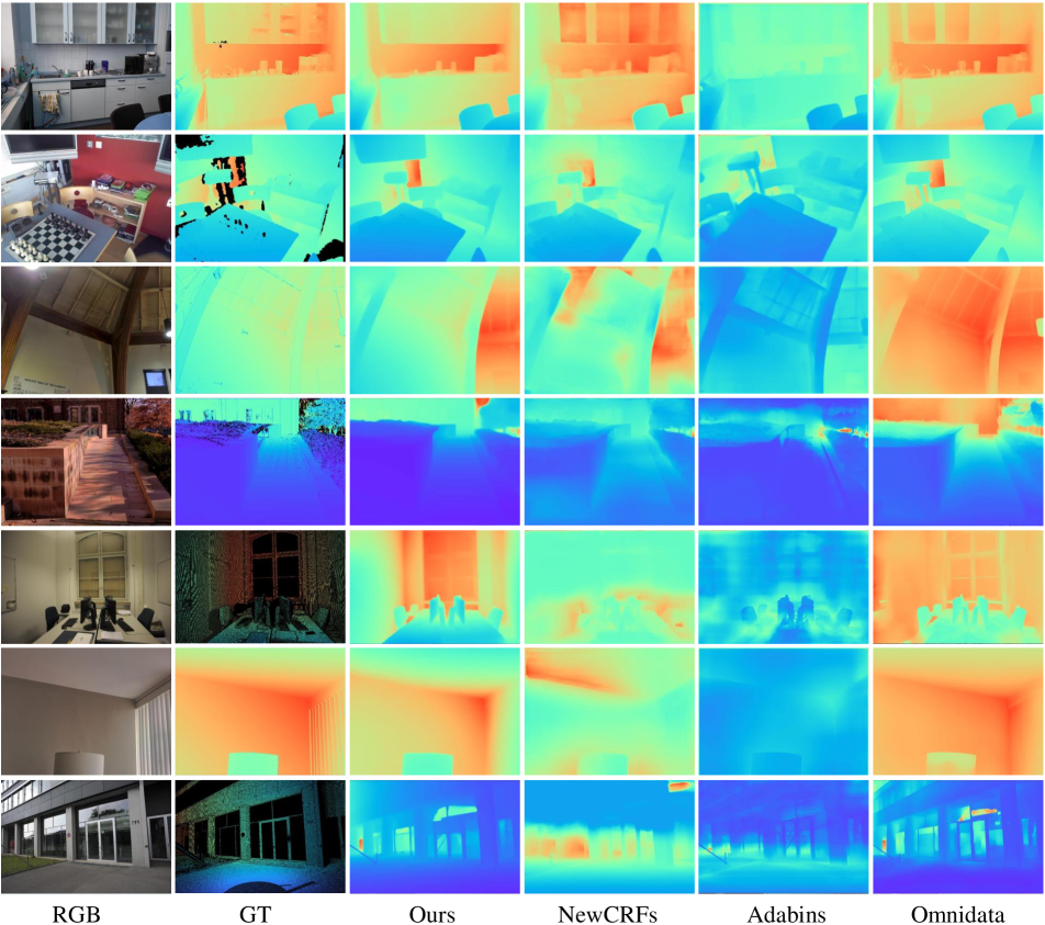
Figure 8: Depth estimation. The visual comparison of predicted on iBims, ETH3D, and DIODE.

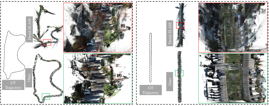
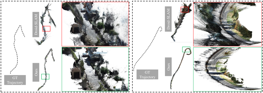
Figure 9: Dense-SLAM Mapping. Existing SOTA mono-SLAM methods usually face scale drift problems in large-scale scenes and are unable to achieve the metric scale. We show the ground-truth trajectory and Droid-SLAM [52] predicted trajectory and their dense mapping. Then, we naively input our metric depth to Droid-SLAM, which can recover a much more accurate trajectory and perform the metric dense mapping.

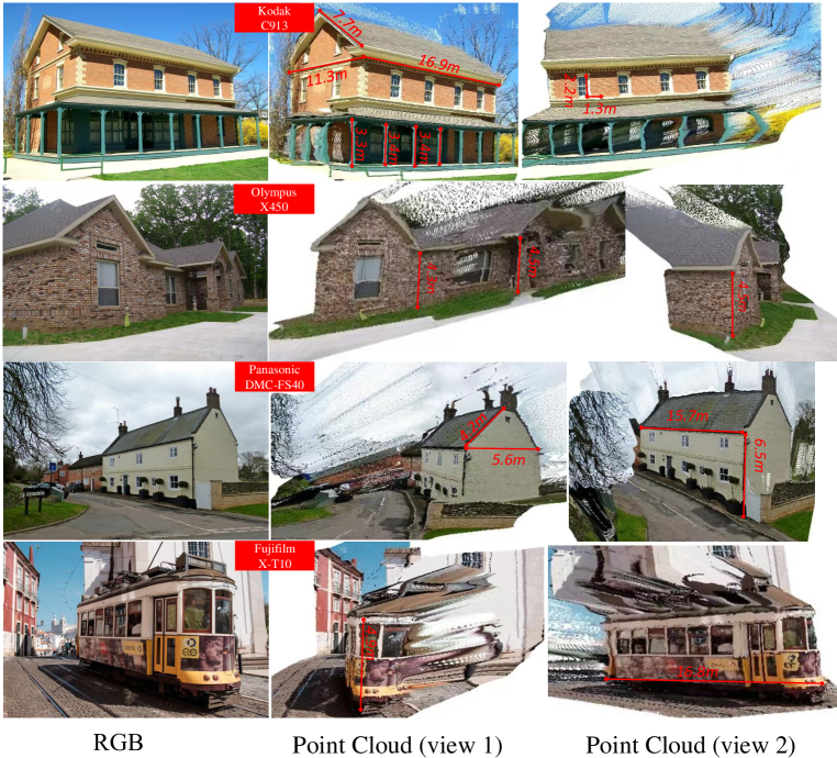
Figure 10: 3D metric reconstruction of in-the-wild images. We collect several Flickr images and use our model to reconstruct the scene. The focal length information is collected from the photo’s metadata. From the reconstructed point cloud, we can measure some structures’ sizes. We can observe that sizes are in a reasonable range.

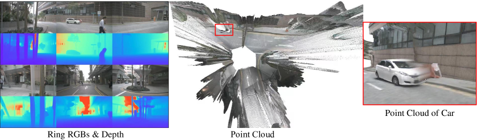
Figure 11: 3D reconstruction of 360°views. Current autonomous driving cars are equipped with several pin-hole cameras to capture 360°views. With our model, we can reconstruct each view and smoothly fuse them together. We can see that all views can be well merged together without scale inconsistency problems. Testing data are from NuScenes. Note that the front view camera has a different focal length from other views.

Figure 12: Depth estimation. The visual comparison of predicted on iBims, ETH3D, and DIODE.

Figure 13: Depth estimation. The visual comparison of predicted on iBims, ETH3D, and DIODE.

Figure 14: Depth estimation. The visual comparison of predicted on iBims, ETH3D, and DIODE.

References

- [1] Jonathan T Barron and Jitendra Malik. Shape, illumination, and reflectance from shading. IEEE Trans. Pattern Anal. Mach. Intell., 37(8):1670–1687, 2014.
- [2] Zuria Bauer, Francisco Gomez-Donoso, Edmanuel Cruz, Sergio Orts-Escolano, and Miguel Cazorla. Uasol, a large-scale high-resolution outdoor stereo dataset. Scientific data, 6(1):1–14, 2019.
- [3] Paul Besl and Neil McKay. Method for registration of 3-d shapes. In Sensor fusion IV: Control Paradigms and Data Structures, volume 1611, pages 586–606. Spie, 1992.
- [4] Shariq Farooq Bhat, Ibraheem Alhashim, and Peter Wonka. Adabins: Depth estimation using adaptive bins. In Proc. IEEE Conf. Comp. Vis. Patt. Recogn., pages 4009–4018, 2021.
- [5] Jia-Wang Bian, Huangying Zhan, Naiyan Wang, Tat-Jin Chin, Chunhua Shen, and Ian Reid. Auto-rectify network for unsupervised indoor depth estimation. IEEE Trans. Pattern Anal. Mach. Intell., 2021.
- [6] Holger Caesar, Varun Bankiti, Alex H Lang, Sourabh Vora, Venice Erin Liong, Qiang Xu, Anush Krishnan, Yu Pan, Giancarlo Baldan, and Oscar Beijbom. nuscenes: A multimodal dataset for autonomous driving. In Proc. IEEE Conf. Comp. Vis. Patt. Recogn., pages 11621–11631, 2020.
- [7] Weifeng Chen, Zhao Fu, Dawei Yang, and Jia Deng. Single-image depth perception in the wild. In Proc. Advances in Neural Inf. Process. Syst., pages 730–738, 2016.
- [8] Weifeng Chen, Shengyi Qian, David Fan, Noriyuki Kojima, Max Hamilton, and Jia Deng. Oasis: A large-scale dataset for single image 3d in the wild. In Proc. IEEE Conf. Comp. Vis. Patt. Recogn., pages 679–688, 2020.
- [9] Jaehoon Cho, Dongbo Min, Youngjung Kim, and Kwanghoon Sohn. DIML/CVL RGB-D dataset: 2m RGB-D images of natural indoor and outdoor scenes. arXiv: Comp. Res. Repository, 2021.
- [10] Marius Cordts, Mohamed Omran, Sebastian Ramos, Timo Rehfeld, Markus Enzweiler, Rodrigo Benenson, Uwe Franke, Stefan Roth, and Bernt Schiele. The cityscapes dataset for semantic urban scene understanding. In Proc. IEEE Conf. Comp. Vis. Patt. Recogn., 2016.
- [11] Angela Dai, Angel X Chang, Manolis Savva, Maciej Halber, Thomas Funkhouser, and Matthias Nießner. Scannet: Richly-annotated 3d reconstructions of indoor scenes. In Proc. IEEE Conf. Comp. Vis. Patt. Recogn., pages 5828–5839, 2017.
- [12] Alexey Dosovitskiy, Lucas Beyer, Alexander Kolesnikov, Dirk Weissenborn, Xiaohua Zhai, Thomas Unterthiner, Mostafa Dehghani, Matthias Minderer, Georg Heigold, Sylvain Gelly, Jakob Uszkoreit, and Neil Houlsby. An image is worth 16x16 words: Transformers for image recognition at scale. Proc. Int. Conf. Learn. Representations, 2021.
- [13] Ainaz Eftekhar, Alexander Sax, Jitendra Malik, and Amir Zamir. Omnidata: A scalable pipeline for making multi-task mid-level vision datasets from 3d scans. In Proc. IEEE Conf. Comp. Vis. Patt. Recogn., pages 10786–10796, 2021.
- [14] David Eigen, Christian Puhrsch, and Rob Fergus. Depth map prediction from a single image using a multi-scale deep network. In Proc. Advances in Neural Inf. Process. Syst., pages 2366–2374, 2014.
- [15] Jose Facil, Benjamin Ummenhofer, Huizhong Zhou, Luis Montesano, Thomas Brox, and Javier Civera. CAM-Convs: camera-aware multi-scale convolutions for single-view depth. In Proc. IEEE Conf. Comp. Vis. Patt. Recogn., pages 11826–11835, 2019.
- [16] Mathias Gehrig, Willem Aarents, Daniel Gehrig, and Davide Scaramuzza. Dsec: A stereo event camera dataset for driving scenarios. IEEE Robotics and Automation Letters, 2021.
- [17] Andreas Geiger, Philip Lenz, Christoph Stiller, and Raquel Urtasun. Vision meets robotics: The kitti dataset. Int. J. Robot. Res., 2013.
- [18] Andreas Geiger, Philip Lenz, and Raquel Urtasun. Are we ready for autonomous driving? the kitti vision benchmark suite. In Proc. IEEE Conf. Comp. Vis. Patt. Recogn., pages 3354–3361. IEEE, 2012.
- [19] Vitor Guizilini, Rares Ambrus, Sudeep Pillai, Allan Raventos, and Adrien Gaidon. 3d packing for self-supervised monocular depth estimation. In Proc. IEEE Conf. Comp. Vis. Patt. Recogn., 2020.
- [20] Xiaoyang Guo, Hongsheng Li, Shuai Yi, Jimmy Ren, and Xiaogang Wang. Learning monocular depth by distilling cross-domain stereo networks. In Proc. Eur. Conf. Comp. Vis., pages 484–500, 2018.
- [21] Richard Hartley and Andrew Zisserman. Multiple view geometry in computer vision. Cambridge university press, 2003.
- [22] Yannick Hold-Geoffroy, Kalyan Sunkavalli, Jonathan Eisenmann, Matthew Fisher, Emiliano Gambaretto, Sunil Hadap, and Jean-François Lalonde. A perceptual measure for deep single image camera calibration. In Proc. IEEE Conf. Comp. Vis. Patt. Recogn., pages 2354–2363, 2018.
- [23] Sunghoon Im, Hae-Gon Jeon, Stephen Lin, and In-So Kweon. Dpsnet: End-to-end deep plane sweep stereo. In Proc. Int. Conf. Learn. Representations, 2019.
- [24] R. Kesten, M. Usman, J. Houston, T. Pandya, K. Nadhamuni, A. Ferreira, M. Yuan, B. Low, A. Jain, P. Ondruska, S. Omari, S. Shah, A. Kulkarni, A. Kazakova, C. Tao, L. Platinsky, W. Jiang, and V. Shet. Level 5 perception dataset 2020. https://level-5.global/level5/data/, 2019.
- [25] Arno Knapitsch, Jaesik Park, Qian-Yi Zhou, and Vladlen Koltun. Tanks and temples: Benchmarking large-scale scene reconstruction. ACM Trans. Graph., 36(4):1–13, 2017.
- [26] Tobias Koch, Lukas Liebel, Friedrich Fraundorfer, and Marco Korner. Evaluation of cnn-based single-image depth estimation methods. In Eur. Conf. Comput. Vis. Worksh., pages 0–0, 2018.
- [27] Johannes Kopf, Xuejian Rong, and Jia-Bin Huang. Robust consistent video depth estimation. In Proc. IEEE Conf. Comp. Vis. Patt. Recogn., 2021.
- [28] Iro Laina, Christian Rupprecht, Vasileios Belagiannis, Federico Tombari, and Nassir Navab. Deeper depth prediction with fully convolutional residual networks. In 2016 Fourth international conference on 3D vision (3DV), pages 239–248. IEEE, 2016.
- [29] John Lambert, Zhuang Liu, Ozan Sener, James Hays, and Vladlen Koltun. Mseg: A composite dataset for multi-domain semantic segmentation. In Proc. IEEE Conf. Comp. Vis. Patt. Recogn., pages 2879–2888, 2020.
- [30] Jun Li, Reinhard Klein, and Angela Yao. A two-streamed network for estimating fine-scaled depth maps from single rgb images. In Proc. IEEE Conf. Comp. Vis. Patt. Recogn., pages 3372–3380, 2017.
- [31] Shunkai Li, Xin Wu, Yingdian Cao, and Hongbin Zha. Generalizing to the open world: Deep visual odometry with online adaptation. In Proc. IEEE Conf. Comp. Vis. Patt. Recogn., pages 13184–13193, 2021.
- [32] Lahav Lipson, Zachary Teed, and Jia Deng. Raft-stereo: Multilevel recurrent field transforms for stereo matching. In Int. Conf. 3D. Vis., 2021.
- [33] Zhuang Liu, Hanzi Mao, Chao-Yuan Wu, Christoph Feichtenhofer, Trevor Darrell, and Saining Xie. A convnet for the 2020s. In Proc. IEEE Conf. Comp. Vis. Patt. Recogn., pages 11976–11986, 2022.
- [34] Manuel Lopez-Antequera, Pau Gargallo, Markus Hofinger, Samuel Rota Bulò, Yubin Kuang, and Peter Kontschieder. Mapillary planet-scale depth dataset. In Proc. Eur. Conf. Comp. Vis., volume 12347, pages 589–604, 2020.
- [35] Raul Mur-Artal and Juan D Tardós. Orb-slam2: An open-source slam system for monocular, stereo, and rgb-d cameras. IEEE transactions on robotics, 33(5):1255–1262, 2017.
- [36] Raúl Mur-Artal and Juan D. Tardós. ORB-SLAM2: an open-source SLAM system for monocular, stereo and RGB-D cameras. IEEE Trans. Robot., 33(5):1255–1262, 2017.
- [37] Sida Peng, Shangzhan Zhang, Zhen Xu, Chen Geng, Boyi Jiang, Hujun Bao, and Xiaowei Zhou. Animatable neural implicit surfaces for creating avatars from videos. arXiv: Comp. Res. Repository, page 2203.08133, 2022.
- [38] Alec Radford, Jong Wook Kim, Chris Hallacy, Aditya Ramesh, Gabriel Goh, Sandhini Agarwal, Girish Sastry, Amanda Askell, Pamela Mishkin, Jack Clark, et al. Learning transferable visual models from natural language supervision. In Proc. Int. Conf. Mach. Learn., pages 8748–8763. PMLR, 2021.
- [39] René Ranftl, Alexey Bochkovskiy, and Vladlen Koltun. Vision transformers for dense prediction. In Proc. IEEE Int. Conf. Comp. Vis., pages 12179–12188, 2021.
- [40] René Ranftl, Katrin Lasinger, David Hafner, Konrad Schindler, and Vladlen Koltun. Towards robust monocular depth estimation: Mixing datasets for zero-shot cross-dataset transfer. IEEE Trans. Pattern Anal. Mach. Intell., 2020.
- [41] Shunsuke Saito, Zeng Huang, Ryota Natsume, Shigeo Morishima, Angjoo Kanazawa, and Hao Li. Pifu: Pixel-aligned implicit function for high-resolution clothed human digitization. In Proc. IEEE Conf. Comp. Vis. Patt. Recogn., pages 2304–2314, 2019.
- [42] Shunsuke Saito, Tomas Simon, Jason Saragih, and Hanbyul Joo. Pifuhd: Multi-level pixel-aligned implicit function for high-resolution 3d human digitization. In Proc. IEEE Conf. Comp. Vis. Patt. Recogn., pages 84–93, 2020.
- [43] Ashutosh Saxena, Min Sun, and Andrew Y Ng. Make3d: Learning 3d scene structure from a single still image. IEEE Trans. Pattern Anal. Mach. Intell., 31(5):824–840, 2008.
- [44] Johannes Lutz Schönberger, Enliang Zheng, Marc Pollefeys, and Jan-Michael Frahm. Pixelwise view selection for unstructured multi-view stereo. In Proc. Eur. Conf. Comp. Vis., 2016.
- [45] Thomas Schops, Johannes L Schonberger, Silvano Galliani, Torsten Sattler, Konrad Schindler, Marc Pollefeys, and Andreas Geiger. A multi-view stereo benchmark with high-resolution images and multi-camera videos. In Proc. IEEE Conf. Comp. Vis. Patt. Recogn., pages 3260–3269, 2017.
- [46] Jamie Shotton, Ben Glocker, Christopher Zach, Shahram Izadi, Antonio Criminisi, and Andrew Fitzgibbon. Scene coordinate regression forests for camera relocalization in rgb-d images. In Proc. IEEE Conf. Comp. Vis. Patt. Recogn., pages 2930–2937, 2013.
- [47] Nathan Silberman, Derek Hoiem, Pushmeet Kohli, and Rob Fergus. Indoor segmentation and support inference from rgbd images. In Proc. Eur. Conf. Comp. Vis., pages 746–760. Springer, 2012.
- [48] Dalwinder Singh and Birmohan Singh. Investigating the impact of data normalization on classification performance. Applied Soft Computing, 2019.
- [49] Shiyu Song, Manmohan Chandraker, and Clark C Guest. High accuracy monocular sfm and scale correction for autonomous driving. IEEE Trans. Pattern Anal. Mach. Intell., 38(4):730–743, 2015.
- [50] Jaime Spencer, C. Stella Qian, Michaela Trescakova, Chris Russell, Simon Hadfield, Erich W. Graf, Wendy J. Adams, Andrew J. Schofield, James Elder, Richard Bowden, Ali Anwar, Hao Chen, Xiaozhi Chen, Kai Cheng, Yuchao Dai, Huynh Thai Hoa, Sadat Hossain, Jianmian Huang, Mohan Jing, Bo Li, Chao Li, Baojun Li, Zhiwen Liu, Stefano Mattoccia, Siegfried Mercelis, Myungwoo Nam, Matteo Poggi, Xiaohua Qi, Jiahui Ren, Yang Tang, Fabio Tosi, Linh Trinh, S. M. Nadim Uddin, Khan Muhammad Umair, Kaixuan Wang, Yufei Wang, Yixing Wang, Mochu Xiang, Guangkai Xu, Wei Yin, Jun Yu, Qi Zhang, and Chaoqiang Zhao. The second monocular depth estimation challenge. In IEEE Conf. Comput. Vis. Pattern Recog. Worksh., pages 3063–3075, June 2023.
- [51] Libo Sun, Wei Yin, Enze Xie, Zhengrong Li, Changming Sun, and Chunhua Shen. Improving monocular visual odometry using learned depth. IEEE Transactions on Robotics, 38(5):3173–3186, 2022.
- [52] Zachary Teed and Jia Deng. Droid-slam: Deep visual slam for monocular, stereo, and rgb-d cameras. volume 34, pages 16558–16569, 2021.
- [53] Igor Vasiljevic, Nick Kolkin, Shanyi Zhang, Ruotian Luo, Haochen Wang, Falcon Z Dai, Andrea F Daniele, Mohammadreza Mostajabi, Steven Basart, Matthew R Walter, et al. Diode: A dense indoor and outdoor depth dataset. arXiv: Comp. Res. Repository, page 1908.00463, 2019.
- [54] Nanyang Wang, Yinda Zhang, Zhuwen Li, Yanwei Fu, Wei Liu, and Yu-Gang Jiang. Pixel2mesh: Generating 3d mesh models from single RGB images. In Proc. Eur. Conf. Comp. Vis., pages 52–67, 2018.
- [55] Benjamin Wilson, William Qi, Tanmay Agarwal, John Lambert, Jagjeet Singh, Siddhesh Khandelwal, Bowen Pan, Ratnesh Kumar, Andrew Hartnett, Jhony Kaesemodel Pontes, Deva Ramanan, Peter Carr, and James Hays. Argoverse 2: Next generation datasets for self-driving perception and forecasting. In Proc. Advances in Neural Inf. Process. Syst., 2021.
- [56] Jiajun Wu, Chengkai Zhang, Xiuming Zhang, Zhoutong Zhang, William Freeman, and Joshua Tenenbaum. Learning shape priors for single-view 3d completion and reconstruction. In Proc. Eur. Conf. Comp. Vis., pages 646–662, 2018.
- [57] Ke Xian, Chunhua Shen, Zhiguo Cao, Hao Lu, Yang Xiao, Ruibo Li, and Zhenbo Luo. Monocular relative depth perception with web stereo data supervision. In Proc. IEEE Conf. Comp. Vis. Patt. Recogn., pages 311–320, 2018.
- [58] Ke Xian, Jianming Zhang, Oliver Wang, Long Mai, Zhe Lin, and Zhiguo Cao. Structure-guided ranking loss for single image depth prediction. In Proc. IEEE Conf. Comp. Vis. Patt. Recogn., pages 611–620, 2020.
- [59] Pengchuan Xiao, Zhenlei Shao, Steven Hao, Zishuo Zhang, Xiaolin Chai, Judy Jiao, Zesong Li, Jian Wu, Kai Sun, Kun Jiang, Yunlong Wang, and Diange Yang. Pandaset: Advanced sensor suite dataset for autonomous driving. In IEEE Int. Intelligent Transportation Systems Conf., 2021.
- [60] Saining Xie, Ross Girshick, Piotr Dollár, Zhuowen Tu, and Kaiming He. Aggregated residual transformations for deep neural networks. In Proc. IEEE Conf. Comp. Vis. Patt. Recogn., pages 1492–1500, 2017.
- [61] Guangkai Xu, Wei Yin, Hao Chen, Chunhua Shen, Kai Cheng, and Feng Zhao. Pose-free 3d scene reconstruction with frozen depth models. In Proc. IEEE Int. Conf. Comp. Vis., 2023.
- [62] Guorun Yang, Xiao Song, Chaoqin Huang, Zhidong Deng, Jianping Shi, and Bolei Zhou. Drivingstereo: A large-scale dataset for stereo matching in autonomous driving scenarios. In Proc. IEEE Conf. Comp. Vis. Patt. Recogn., 2019.
- [63] Guanglei Yang, Hao Tang, Mingli Ding, Nicu Sebe, and Elisa Ricci. Transformer-based attention networks for continuous pixel-wise prediction. In Proc. IEEE Int. Conf. Comp. Vis., 2021.
- [64] Wei Yin, Yifan Liu, and Chunhua Shen. Virtual normal: Enforcing geometric constraints for accurate and robust depth prediction. IEEE Trans. Pattern Anal. Mach. Intell., 2021.
- [65] Wei Yin, Yifan Liu, Chunhua Shen, Anton van den Hengel, and Baichuan Sun. The devil is in the labels: Semantic segmentation from sentences. arXiv: Comp. Res. Repository, page 2202.02002, 2022.
- [66] Wei Yin, Yifan Liu, Chunhua Shen, and Youliang Yan. Enforcing geometric constraints of virtual normal for depth prediction. In Proc. IEEE Int. Conf. Comp. Vis., 2019.
- [67] Wei Yin, Xinlong Wang, Chunhua Shen, Yifan Liu, Zhi Tian, Songcen Xu, Changming Sun, and Dou Renyin. Diversedepth: Affine-invariant depth prediction using diverse data. arXiv: Comp. Res. Repository, page 2002.00569, 2020.
- [68] Wei Yin, Jianming Zhang, Oliver Wang, Simon Niklaus, Simon Chen, Yifan Liu, and Chunhua Shen. Towards accurate reconstruction of 3d scene shape from a single monocular image. IEEE Trans. Pattern Anal. Mach. Intell., 2022.
- [69] Wei Yin, Jianming Zhang, Oliver Wang, Simon Niklaus, Long Mai, Simon Chen, and Chunhua Shen. Learning to recover 3d scene shape from a single image. In Proc. IEEE Conf. Comp. Vis. Patt. Recogn., 2021.
- [70] Zhichao Yin and Jianping Shi. Geonet: Unsupervised learning of dense depth, optical flow and camera pose. In Proceedings of the IEEE conference on computer vision and pattern recognition, pages 1983–1992, 2018.
- [71] Weihao Yuan, Xiaodong Gu, Zuozhuo Dai, Siyu Zhu, and Ping Tan. New CRFs: Neural window fully-connected CRFs for monocular depth estimation. In Proc. IEEE Conf. Comp. Vis. Patt. Recogn., 2022.
- [72] Amir Zamir, Alexander Sax, , William Shen, Leonidas Guibas, Jitendra Malik, and Silvio Savarese. Taskonomy: Disentangling task transfer learning. In Proc. IEEE Conf. Comp. Vis. Patt. Recogn. IEEE, 2018.
- [73] Chi Zhang, Wei Yin, Zhibin Wang, Gang Yu, Bin Fu, and Chunhua Shen. Hierarchical normalization for robust monocular depth estimation. Proc. Advances in Neural Inf. Process. Syst., 2022.
- [74] Chi Zhang, Wei Yin, Gang Yu, Zhibin Wang, Tao Chen, Bin Fu, Joey Tianyi Zhou, and Chunhua Shen. Robust geometry-preserving depth estimation using differentiable rendering. In Proc. IEEE Int. Conf. Comp. Vis., 2023.
- [75] Rui Zhu, Xingyi Yang, Yannick Hold-Geoffroy, Federico Perazzi, Jonathan Eisenmann, Kalyan Sunkavalli, and Manmohan Chandraker. Single view metrology in the wild. In Proc. Eur. Conf. Comp. Vis., pages 316–333. Springer, 2020.