Denoising of Sphere- and SO(3)-Valued Data by Relaxed Tikhonov Regularization

Abstract

Manifold-valued signal- and image processing has received attention due to modern image acquisition techniques. Recently, Condat (IEEE Trans. Signal Proc.) proposed a convex relaxation of the Tikhonov-regularized nonconvex problem for denoising circle-valued data. Using Schur complement arguments, we show that this variational model can be simplified while leading to the same solution. Our simplified model can be generalized to higher dimensional spheres and to ${\mathrm{SO}}(3)$-valued data, where we rely on the quaternion representation of the latter. Standard algorithms from convex analysis can be applied to solve the resulting convex minimization problem. As proof-of-the-concept, we use the alternating direction method of minimizers to demonstrate the denoising behavior of the proposed approach.

I Introduction

With the emergence of modern acquisition techniques which produce manifold-valued signals and images, research in this field focuses new challenges. Circle-valued data appear in interferometric synthetic aperture radar [1, 2, 3], color image restoration in HSV or LCh spaces [4], Magnetic Resonance Imaging [5], biology [6], psychology [7] and various other applications involving the phase of Fourier transformed data for instance. Signals and images with values on the 2-sphere play a role when dealing with 3d directional information [8, 9, 10] or in the processing of color images in the chromaticity-brightness setting [11, 12, 13]. The rotation group ${\mathrm{SO}}(3)$ was considered in tracking and motion analysis and in the analysis of back scatter diffraction data (EBSD) [14, 15, 16].

The denoising of circle- and sphere-valued data was addressed by several methods as lifting procedures [17, 18, 19], variational approaches with TV-like regularizers [20, 21] and half-quadratic minimization models like the iteratively re-weighted least squares method [22, 23]. These methods either enlarge the dimension of the problem drastically, especially for lifting methods, have restricted convergence guarantees, or rely on data on Hadamard manifolds, which spheres are not. There are few stochastic approaches in manifold-valued data processing as the work of Pennec’s group, see for instance [24, 25], where a patch-based approach via an MMSE model on the respective manifold is applied. For an overview, we also refer to [26].

In this paper, we focus exclusively on the important simple variational model with quadratic Tikhonov regularization that penalizes the squared differences of adjacent values on a graph, which promotes the property that such values are close to each other. Unfortunately, due to the manifold constrained, this is still a difficult nonconvex problem. Recalling the convexity relaxed model of Condat [27] for circle-valued data, we show how this relaxed model can be nicely simplified without loosing any information. Based on Schur complement arguments, we will see that our model leads to the same minimizers while reducing the number of parameters and consequently making the computation more efficient. In a preprint [28], which came without any numerical results, Condat suggested to generalize his model to data on the 2-sphere. In this paper, we will see that this approach can be simplified as well. Moreover, it just appears as a special case of quaternion-valued data processing. The latter one also leads to a relaxed convex model for ${\mathrm{SO}}(3)$-valued data.

Outline of the paper: in Section II, we reconsider Condat’s relaxation of the nonconvex Tikhonov model for denoising circle-valued data. We address the model from two different points of view depending whether we embed the circle into the complex numbers $\mathbb{C}$ or into the real numbers $\mathbb{R}^{2}$. Both view points make it easier to understand the later extension of the approach to the quaternion setting. Then, we introduce our simplified model and prove that this model has the same solutions as original relaxed formulation by using Schur complement arguments. In Section III, we will see that our simplified model can be generalized to higher dimensional spheres in a straightforward way. Next, in Section IV, we explain how the nonconvex Tikhonov model as well as its relaxation and simplification can be generalized to ${\mathrm{SO}}(3)$-valued data. The approach relies on the parameterization of ${\mathrm{SO}}(3)$ by quaternions. Remarkably, it also includes 2-sphere-valued data. We describe the ADMM for finding a minimizer of our relaxed models in Section V. Finally, Section VI provides some proof-of-the-concept denoising examples for circle-, sphere- and ${\mathrm{SO}}(3)$-valued data.

II Denoising of Circle-Valued Data

Let $G=(V,E)$ be a connected, undirected graph, where $V\coloneqq\{1,\dots,N\}$ denotes the set of vertices, and $E\subset\{(n,m)\in V\times V:n<m\}$ the set of edges. The cardinality of $E$ is henceforth denoted by $M\coloneqq\lvert E\rvert$. Our aim is to denoise a disturbed circle-valued signal on $G$. The circle can be either embedded into the complex numbers $\mathbb{C}$ or into the two-dimensional Euclidean space $\mathbb{R}^{2}$. The former approach has been especially considered by Condat [27]. The latter approach proposed by us can be immediately generalized to tackle sphere-valued and ${\mathrm{SO}}(3)$-valued data.

II-A $\mathbb{C}$-Valued Model

Let $\mathbb{S}_{\mathbb{C}}\coloneqq\{z\in\mathbb{C}:\lvert z\rvert=1\}$ denote the (complex-valued) unit circle. Our aim is to recover an $\mathbb{S}_{\mathbb{C}}$-valued signal $x\coloneqq(x_{n})_{n\in V}\in\mathbb{S}_{\mathbb{C}}^{N}$ on $G$ from noisy measurements $y\coloneqq(y_{n})_{n\in V}\in{\mathbb{S}_{\mathbb{C}}}^{N}$. Note that the following considerations work also for $y\in{\mathbb{C}}^{N}$. A straightforward approach would be to search for the minimizer of the Tikhonov-like regularized functional

$$\operatorname*{arg\,min}_{x\in\mathbb{S}_{\mathbb{C}}^{N}}\sum_{n\in V}\frac{w_{n}}{2}\,\lvert x_{n}-y_{n}\rvert^{2}+\smashoperator[]{\sum_{(n,m)\in E}^{}}\frac{\lambda_{(n,m)}}{2}\,\lvert x_{n}-x_{m}\rvert^{2},$$ (1)

where $w\coloneqq(w_{n})_{n\in V}\in\mathbb{R}^{N}_{+}$ and $\lambda\coloneqq(\lambda_{(n,m)})_{(n,m)\in E}\in\mathbb{R}^{M}_{+}$ are positive weights. Unfortunately, due to the constraints $x_{n}\in\mathbb{S}_{\mathbb{C}}$ , this problem is nonconvex. In the first step, to derive a convex relaxation, we exploit $\lvert x_{n}\rvert=1$ and rewrite the original problem (1) as

$$\operatorname*{arg\,min}_{x\in\mathbb{S}_{\mathbb{C}}^{N}}\,-\sum_{n\in V}w_{n}\,\Re[x_{n}\bar{y}_{n}]\,-\smashoperator[]{\sum_{(n,m)\in E}^{}}\lambda_{(n,m)}\,\Re[\bar{x}_{m}x_{n}].$$ (2)

Introducing $r\coloneqq(r_{(n,m)})_{(n,m)\in E}\in\mathbb{C}^{M}$, we rearrange the minimization problem (2) into

$$\operatorname*{arg\,min}_{x\in\mathbb{S}_{\mathbb{C}}^{N},r\in\mathbb{C}^{M}}\!\!\!\mathcal{J}(x,r)\text{ s.t. }r_{(n,m)}=\bar{x}_{m}x_{n}$$ (3)

for all $(n,m)\in E$ with

$$\mathcal{J}(x,r)\coloneqq-\sum_{n\in V}w_{n}\,\Re[x_{n}\bar{y}_{n}]-\smashoperator[]{\sum_{(n,m)\in E}^{}}\lambda_{(n,m)}\,\Re[r_{(n,m)}].$$ (4)

The core idea of Condat’s convex relaxation [27] is to encode the nonconvex constraint $x\in\mathbb{S}_{\mathbb{C}}^{N}$ into a positive semi-definite, rank-one matrix.

Lemma 1.

Let $n,m\in V$ and $(n,m)\in E$. Then $x_{n},x_{m}\in\mathbb{S}_{\mathbb{C}}$ and $r_{(n,m)}=\bar{x}_{m}x_{n}$ if and only if

$$P_{(n,m)}\coloneqq\begin{bmatrix}1&x_{n}&x_{m}\\ \bar{x}_{n}&1&\bar{r}_{(n,m)}\\ \bar{x}_{m}&r_{(n,m)}&1\end{bmatrix}\in\mathbb{C}^{3\times 3}$$ (5)

is positive semi-definite and has rank one.

Proof.

Let $x_{n},x_{m}\in\mathbb{S}_{\mathbb{C}}$ and $r_{(n,m)}=\bar{x}_{m}x_{n}$, and denote the conjugation and transposition by $\cdot^{\mathrm{H}}$. Then $P_{(n,m)}=(1,x_{n},x_{m})^{\mathrm{H}}(1,x_{n},x_{m})$ has rank one and is positive semi-definite. Conversely, positive semi-definitness and the rank-one condition imply that $P_{(n,m)}$ has the form

$$P_{(n,m)}=(a,b,c)^{\mathrm{H}}(a,b,c)=\begin{bmatrix}\bar{a}a&\bar{a}b&\bar{a}c\\ \bar{b}a&\bar{b}b&\bar{b}a\\ \bar{c}a&\bar{c}b&\bar{c}c\end{bmatrix}$$

for some $a,b,c\in\mathbb{C}$. Comparison with (5) yields $|a|=|b|=|c|=1$ and thus $|x_{n}|=|\bar{a}||b|=1$, $|x_{m}|=|\bar{a}||c|=1$ as well as $r_{(n,m)}=\bar{c}b=\bar{c}a\bar{a}b=\bar{x}_{m}x_{n}$. ∎

We denote the rank function by $\operatorname{rk}$. Based on Lemma 1, Problem (3) and thus the original formulation (1) become

$$\operatorname*{arg\,min}_{x\in\mathbb{C}^{N},r\in\mathbb{C}^{M}}\mathcal{J}(x,r)\text{ s.t. }P_{(n,m)}\succeq 0\;\text{and}\;\operatorname{rk}(P_{(n,m)})=1$$ (6)

for all $(n,m)\in E$. Neglecting the rank-one constraint, Condat [27] proposes to solve the relaxation:

relaxed complex model

$$\operatorname*{arg\,min}_{x\in\mathbb{C}^{N},r\in\mathbb{C}^{M}}\mathcal{J}(x,r)\quad\text{s.t.}\quad P_{(n,m)}\succeq 0$$ (7)

for all $(n,m)\in E$. Since (II-A) is a convex optimization problem, we may apply standard methods from convex analysis to obtain numerical solutions.

II-B Related $\mathbb{R}^{2}$-Valued Model

Alternatively, the sphere can be embedded in the Euclidean space $\mathbb{R}^{2}$ equipped with the Euclidean norm $\lVert\cdot\rVert$ and inner product $\langle\cdot,\cdot\rangle$. To emphasize the relation to the complex-valued model, we identify the complex number $z\in\mathbb{C}$ with the two-dimensional Euclidean vector $\bm{z}\coloneqq(\Re[z],\Im[z])^{\mathrm{T}}\in\mathbb{R}^{2}$, where $\cdot^{\mathrm{T}}$ denotes the transposition. Against this background, we denote the first and second component of $\bm{z}$ by $\Re[\bm{z}]\coloneqq\bm{z}_{1}$ and $\Im[\bm{z}]\coloneqq\bm{z}_{2}$ respectively. Defining $\mathbb{S}_{1}\coloneqq\{\bm{z}\in\mathbb{R}^{2}:\lVert\bm{z}\rVert=1\}$, we now want to recover an $\mathbb{S}_{1}$-valued signal $\bm{x}\coloneqq(\bm{x}_{n})_{n\in V}\in\mathbb{S}_{1}^{N}$ on $G$ from noisy measurements $\bm{y}\coloneqq(\bm{y}_{n})_{n\in V}\in(\mathbb{S}_{1})^{N}$. Exploiting $\lvert z\rvert=\lVert\bm{z}\rVert$ for all $z\in\mathbb{C}$, we rewrite (1) into the real-valued model

$$\operatorname*{arg\,min}_{\bm{x}\in\mathbb{S}_{1}^{N}}\sum_{n\in V}\frac{w_{n}}{2}\,\lVert\bm{x}_{n}-\bm{y}_{n}\rVert^{2}+\smashoperator[]{\sum_{(n,m)\in E}^{}}\frac{\lambda_{(n,m)}}{2}\,\lVert\bm{x}_{n}-\bm{x}_{m}\rVert^{2}.$$ (8)

To transfer the relaxation of the complex model, we exploit that the complex multiplication can be realized using the matrix representation of $z\in\mathbb{C}$ given by

$$\bm{M}(z)\coloneqq\bm{M}(\bm{z})\coloneqq\left[\begin{smallmatrix}\Re[\bm{z}]&-\Im[\bm{z}]\\ \Im[\bm{z}]&\Re[\bm{z}]\end{smallmatrix}\right].$$ (9)

Introducing the variables $\bm{r}_{(n,m)}=\bm{M}(\bm{x}_{m})^{\mathrm{T}}\bm{x}_{n}\in\mathbb{R}^{2}$, the real-valued version of (3) reads as

$$\operatorname*{arg\,min}_{\bm{x}\in\mathbb{S}_{1}^{N},\bm{r}\in(\mathbb{R}^{2})^{M}}\mathcal{J}(\bm{x},\bm{r})\quad\text{s.t.}\quad\bm{r}_{(n,m)}=\bm{M}(\bm{x}_{m})^{\mathrm{T}}\bm{x}_{n}$$ (10)

for all $(n,m)\in E$ with

$$\mathcal{J}(\bm{x},\bm{r})\coloneqq-\sum_{n\in V}w_{n}\,\langle\bm{x}_{n},{\bm{y}}_{n}\rangle-\smashoperator[]{\sum_{(n,m)\in E}^{}}\lambda_{(n,m)}\,\Re[\bm{r}_{(n,m)}].$$ (11)

Denoting the $d\times d$ identity matrix by $\bm{I}_{d}$, where the index is omitted if the dimension is clear, we analogously encode the nonconvex constraint of (10) into a matrix expression.

Lemma 2.

Let $n,m\in V$ and $(n,m)\in E$. Then $\bm{x}_{n},\bm{x}_{m}\in\mathbb{S}_{1}$ and $\bm{r}_{(n,m)}=\bm{M}(\bm{x}_{m})^{\mathrm{T}}\bm{x}_{n}$ if and only if the block matrix

$$\bm{P}_{(n,m)}\coloneqq\left[\begin{smallmatrix}\bm{I}_{2}&\bm{M}(\bm{x}_{n})&\bm{M}(\bm{x}_{m})\\ \bm{M}(\bm{x}_{n})^{\mathrm{T}}&\bm{I}_{2}&\bm{M}(\bm{r}_{(n,m)})^{\mathrm{T}}\\ \bm{M}(\bm{x}_{m})^{\mathrm{T}}&\bm{M}(\bm{r}_{(n,m)})&\bm{I}_{2}\end{smallmatrix}\right]\in\mathbb{R}^{6\times 6}$$ (12)

is positive semi-definite and has rank two.

Proof.

Let the conditions for $\bm{x}_{n},\bm{x}_{m}$ and $\bm{r}_{(n,m)}$ be fulfilled. Since $\bm{M}(\bm{x}_{n})^{\mathrm{T}}\bm{M}(\bm{x}_{n})=\lVert\bm{x}_{n}\rVert^{2}\bm{I}_{2}$ and $\bm{M}(\bm{x}_{m})^{\mathrm{T}}\bm{M}(\bm{x}_{n})=\bm{M}(\bm{r}_{(n,m)})$, we obtain

$$\bm{P}_{(n,m)}=[\bm{I}_{2},\bm{M}(\bm{x}_{n}),\bm{M}(\bm{x}_{m})]^{\mathrm{T}}[\bm{I}_{2},\bm{M}(\bm{x}_{n}),\bm{M}(\bm{x}_{m})]$$

implying $\operatorname{rk}(\bm{P}_{(n,m)})=2$ and $\bm{P}_{(n,m)}\succeq 0$. The opposite direction follows similarly as in the proof of Lemma 1. ∎

Due to Lemma 2, the real-valued formulation (10) becomes

$$\smashoperator[]{\operatorname*{arg\,min}_{\begin{subarray}{c}\bm{x}\in(\mathbb{R}^{2})^{N}\\ \bm{r}\in(\mathbb{R}^{2})^{M}\end{subarray}}^{}}\mathcal{J}(\bm{x},\bm{r})\text{ s.t. }\bm{P}_{(n,m)}\succeq 0\text{ and }\operatorname{rk}(\bm{P}_{(n,m)})=2$$ (13)

for all $(n,m)\in E$. Since obviously $\bm{P}_{(n,m)}\succeq 0$ if and only if $P_{(n,m)}\succeq 0$, neglecting the rank-two constraint in (13) yields the relaxed formulation:

relaxed real model

$$\operatorname*{arg\,min}_{\bm{x}\in(\mathbb{R}^{2})^{N},\bm{r}\in(\mathbb{R}^{2})^{M}}\mathcal{J}(\bm{x},\bm{r})\quad\text{s.t.}\quad\bm{P}_{(n,m)}\succeq 0$$ (14)

for all $(n,m)\in E$, which is just the real-valued version of complex relaxation (II-A).

II-C Simplified $\mathbb{R}^{2}$-Valued Model

Note that the seconds variables $\bm{r}_{(n,m)}=\bm{M}(\bm{x}_{m})^{\mathrm{T}}\bm{x}_{n}$ in (10) are artificial and originate form the complex-valued model. Therefore the minimization problem (10) seems to be needlessly puffed-up since we also optimize with respect to the variables $\Im(\bm{r}_{(n,m)})$ that do not influence the objective $\mathcal{J}$ in (11) at all. To this end, we propose to reformulate the real-valued problem (8) as

$$\operatorname*{arg\,min}_{\bm{x}\in\mathbb{S}_{1}^{N},\bm{\ell}\in\mathbb{R}^{M}}\mathcal{K}(\bm{x},\bm{\ell})\quad\text{s.t.}\quad\bm{\ell}_{(n,m)}=\langle\bm{x}_{n},\bm{x}_{m}\rangle$$ (15)

for all $(n,m)\in E$ with

$$\mathcal{K}(\bm{x},\bm{\ell})\coloneqq-\sum_{n\in V}w_{n}\,\langle\bm{x}_{n},\bm{y}_{n}\rangle-\smashoperator[]{\sum_{(n,m)\in E}^{}}\lambda_{(n,m)}\,\bm{\ell}_{(n,m)}.$$ (16)

As before and with a similar proof, the nonconvex constraints $\bm{x}_{n}\in\mathbb{S}_{1}$ and $\bm{\ell}_{(n,m)}=\langle\bm{x}_{n},\bm{x}_{m}\rangle$ may be encoded using the positive semi-definiteness and a rank condition of an appropriate matrix.

Lemma 3.

Let $n,m\in V$ and $(n,m)\in E$. Then $\bm{x}_{n},\bm{x}_{m}\in\mathbb{S}_{1}$ and $\bm{\ell}_{(n,m)}=\langle\bm{x}_{n},\bm{x}_{m}\rangle$ if and only if the block matrix

$$\bm{Q}_{(n,m)}\coloneqq\begin{bmatrix}\bm{I}_{2}&\bm{x}_{n}&\bm{x}_{m}\\ \bm{x}_{n}^{\mathrm{T}}&1&\bm{\ell}_{(n,m)}\\ \bm{x}_{m}^{\mathrm{T}}&\bm{\ell}_{(n,m)}&1\end{bmatrix}\in\mathbb{R}^{4\times 4}$$ (17)

is positive semi-definite and has rank two.

In this paper, we relax the rank-two constraint and propose to solve our new relaxed formulation:

simplified relaxed real model (18)

$$\operatorname*{arg\,min}_{\bm{x}\in(\mathbb{R}^{2})^{N},\bm{\ell}\in\mathbb{R}^{M}}\mathcal{K}(\bm{x},\bm{\ell})\quad\text{s.t.}\quad\bm{Q}_{(n,m)}\succeq 0$$ (19)

for all $(n,m)\in E$. Our convex model (19) is simpler than (II-B), since $\bm{r}_{(n,m)}\in\mathbb{R}^{2}$ is replaced by $\bm{\ell}_{(n,m)}\in\mathbb{R}$. Nevertheless, both problems lead to the same solutions. To show this, we need a result on the Schur complement of matrices.

Proposition 4 ([29, p. 495]).

For invertible $\bm{A}$, it holds

$$\bm{W}=\left[\begin{smallmatrix}\bm{A}&\bm{C}\\ \bm{C}^{\mathrm{T}}&\bm{B}\end{smallmatrix}\right]=\left[\begin{smallmatrix}\bm{I}&\bm{0}\\ \bm{C}^{\mathrm{T}}\bm{A}^{-1}&\bm{I}\end{smallmatrix}\right]\left[\begin{smallmatrix}\bm{A}&\bm{0}\\ \bm{0}&\bm{B}-\bm{C}^{\mathrm{T}}\bm{A}^{-1}\bm{C}\end{smallmatrix}\right]\left[\begin{smallmatrix}\bm{I}&\bm{A}^{-1}\bm{C}\\ \bm{0}^{\mathrm{T}}&\bm{I}\end{smallmatrix}\right].$$

The matrix $\bm{W}/\bm{A}\coloneqq\bm{B}-\bm{C}^{\mathrm{T}}\bm{A}^{-1}\bm{C}$ is called Schur complement of $\bm{W}$ and we have $\bm{W}\succeq 0$ if and only if $\bm{A}\succ 0$ and $\bm{W}/\bm{A}\succeq 0$.

Now we can prove the main equivalence theorem.

Theorem 5.

Problems (II-B) and (19) are equivalent in the following sense:

1. If $(\hat{\bm{x}},\hat{\bm{r}})$ solves (II-B), then $(\hat{\bm{x}},\Re[\hat{\bm{r}}])$ solves (19).

2. If $(\tilde{\bm{x}},\tilde{\bm{\ell}})$ solves (19), then $(\tilde{\bm{x}},\tilde{\bm{r}})$ with
   $\tilde{\bm{r}}_{(n,m)}=(\tilde{\bm{\ell}}_{(n,m)},\Im[\bm{M}(\tilde{\bm{x}}_{m})^{\mathrm{T}}\tilde{\bm{x}}_{n}])^{\mathrm{T}}$ solves (II-B).

Proof.

The Schur complement of $\bm{Q}_{m,n}$ with respect to $\bm{I}_{2}$ is given by

$$\bm{Q}_{(n,m)}/\bm{I}_{2}=\left[\begin{smallmatrix}1-\lvert\bm{x}_{n}\rvert^{2}&\bm{\ell}_{(n,m)}-\langle\bm{x}_{n},\bm{x}_{m}\rangle\\ \bm{\ell}_{(n,m)}-\langle\bm{x}_{n},\bm{x}_{m}\rangle&1-\lvert\bm{x}_{m}\rvert^{2}\end{smallmatrix}\right]$$ (20)

On the other hand, permuting the fourth and fifth column/row of $\bm{P}_{(n,m)}$, we obtain $\tilde{\bm{P}}_{(n,m)}$ in (27), which has the Schur complement (32), see next page.

$$\tilde{\bm{P}}_{(n,m)}\coloneqq{\small\left[\scalebox{0.75}{ $\begin{array}[]{cc|cc|cc}1&0&\Re[\bm{x}_{n}]&\Re[\bm{x}_{m}]&-\Im[\bm{x}_{n}]&-\Im[\bm{x}_{m}]\\ 0&1&\Im[\bm{x}_{n}]&\Im[\bm{x}_{m}]&\Re[\bm{x}_{n}]&\Re[\bm{x}_{m}]\\ \hline\cr\Re[\bm{x}_{n}]&\Im[\bm{x}_{n}]&1&\Re[\bm{r}_{(n,m)}]&0&\Im[\bm{r}_{(n,m)}]\\ \Re[\bm{x}_{m}]&\Im[\bm{x}_{m}]&\Re[\bm{r}_{(n,m)}]&1&-\Im[\bm{r}_{(n,m)}]&0\\ \hline\cr-\Im[\bm{x}_{n}]&\Re[\bm{x}_{n}]&0&-\Im[\bm{r}_{(n,m)}]&1&\Re[\bm{r}_{(n,m)}]\\ -\Im[\bm{x}_{m}]&\Re[\bm{x}_{m}]&\Im[\bm{r}_{(n,m)}]&0&\Re[\bm{r}_{(n,m)}]&1\end{array}$}\right],}$$ (27)

$$\tilde{\bm{P}}_{(n,m)}/\bm{I}_{2}=\left[\scalebox{0.75}{ $\begin{array}[]{cc|cc}1-\lvert\bm{x}_{n}\rvert^{2}&\Re[\bm{r}_{(n,m)}]-\Re[\bm{M}(\bm{x}_{m})^{\mathrm{T}}\bm{x}_{n}]&0&\Im[\bm{r}_{(n,m)}]-\Im[\bm{M}(\bm{x}_{m})^{\mathrm{T}}\bm{x}_{n}]\\ \Re[\bm{r}_{(n,m)}]-\Re[\bm{M}(\bm{x}_{m})^{\mathrm{T}}\bm{x}_{n}]&1-\lvert\bm{x}_{m}\rvert^{2}&-\Im[\bm{r}_{(n,m)}]+\Im[\bm{M}(\bm{x}_{m})^{\mathrm{T}}\bm{x}_{n}]&0\\ \hline\cr 0&-\Im[\bm{r}_{(n,m)}]+\Im[\bm{M}(\bm{x}_{m})^{\mathrm{T}}\bm{x}_{n}]&1-\lvert\bm{x}_{n}\rvert^{2}&\Re[\bm{r}_{(n,m)}]-\Re[\bm{M}(\bm{x}_{m})^{\mathrm{T}}\bm{x}_{n}]\\ \Im[\bm{r}_{(n,m)}]-\Im[\bm{M}(\bm{x}_{m})^{\mathrm{T}}\bm{x}_{n}]&0&\Re[\bm{r}_{(n,m)}]-\Re[\bm{M}(\bm{x}_{m})^{\mathrm{T}}\bm{x}_{n}]&1-\lvert\bm{x}_{m}\rvert^{2}\end{array}$}\right]\!\!.$$ (32)

Recall that $\Re[\bm{M}(\bm{x}_{m})^{\mathrm{T}}\bm{x}_{n}]=\langle\bm{x}_{n},\bm{x}_{m}\rangle$. Using the Schur complements in (20) and (32) as well as Proposition 4, we obtain the following: if $(\hat{\bm{x}},\hat{\bm{r}})$ solves (II-B), then $(\hat{\bm{x}},\hat{\bm{\ell}})$ with $\hat{\bm{\ell}}\coloneqq\Re[\hat{\bm{r}}]$ is a feasible point of (19). Moreover, it holds by their definition that $\mathcal{K}(\hat{\bm{x}},\hat{\bm{\ell}})=\mathcal{J}(\hat{\bm{x}},\hat{\bm{r}})$.

Conversely, if $(\tilde{\bm{x}},\tilde{\bm{\ell}})$ solves (19), then $(\tilde{\bm{x}},\tilde{\bm{r}})$ with $\tilde{\bm{r}}$ defined in the theorem is a feasible point of (II-B). Further, we have $\mathcal{K}(\tilde{\bm{x}},\tilde{\bm{\ell}})=\mathcal{J}(\tilde{\bm{x}},\tilde{\bm{r}})$. Taking the minimizing property into account, we conclude

$$\mathcal{K}(\tilde{\bm{x}},\tilde{\bm{\ell}})\leq\mathcal{K}(\hat{\bm{x}},\hat{\bm{\ell}})=\mathcal{J}(\hat{\bm{x}},\hat{\bm{r}})\leq\mathcal{J}(\tilde{\bm{x}},\tilde{\bm{r}})=\mathcal{K}(\tilde{\bm{x}},\tilde{\bm{\ell}}),$$

which is only possible if all values coincides. ∎

Our previous considerations yield immediately the following corollary.

Corollary 6.

Problems (II-A) and (19) are equivalent in the following sense:

1. If $(\hat{x},\hat{r})$ solves (II-A), then $(\hat{\bm{x}},\Re[\hat{r}])$ solves (19).

2. If $(\tilde{\bm{x}},\tilde{\bm{\ell}})$ solves (19), then $(\tilde{x},\tilde{r})$ with
   $\tilde{r}_{(n,m)}=\tilde{\bm{\ell}}_{(n,m)}+\mathrm{i}\Im[\overline{\tilde{x}}_{m}\tilde{x}_{n}]$ solves (II-B).

III Generalization to Sphere-Valued Data

The main advantage of the real-valued, relaxed model (19) is its simple generalization to higher dimensions. Defining the $(d-1)$-dimensional sphere as $\mathbb{S}_{d-1}\coloneqq\{\bm{x}\in\mathbb{R}^{d}:\lVert\bm{x}\rVert=1\}$, we aim to determine the signal $\bm{x}\coloneqq(\bm{x}_{n})_{n\in V}\in\mathbb{S}_{d-1}^{N}$ on $G$ from perturbed values $\bm{y}\coloneqq(\bm{y}_{n})_{n\in V}\in(\mathbb{S}_{d-1})^{N}$. For this, we start with the original, nonconvex problem

$$\operatorname*{arg\,min}_{\bm{x}\in\mathbb{S}_{d-1}^{N}}\sum_{n\in V}\frac{w_{n}}{2}\,\lVert\bm{x}_{n}-\bm{y}_{n}\rVert^{2}+\smashoperator[]{\sum_{(n,m)\in E}^{}}\frac{\lambda_{(n,m)}}{2}\,\lVert\bm{x}_{n}-\bm{x}_{m}\rVert^{2},$$ (33)

and its rewritten version

$$\operatorname*{arg\,min}_{\bm{x}\in\mathbb{S}_{d-1}^{N},\bm{\ell}\in\mathbb{R}^{M}}\mathcal{K}(\bm{x},\bm{\ell})\quad\text{s.t.}\quad\bm{\ell}_{(n,m)}=\langle\bm{x}_{n},\bm{x}_{m}\rangle$$ (34)

for all $(n,m)\in E$ with

$$\mathcal{K}(\bm{x},\bm{\ell})\coloneqq-\sum_{n\in V}w_{n}\,\langle\bm{x}_{n},\bm{y}_{n}\rangle-\smashoperator[]{\sum_{(n,m)\in E}^{}}\lambda_{(n,m)}\,\bm{\ell}_{(n,m)}.$$ (35)

Immediately, Lemma 3 extends to higher dimensions as follows.

Lemma 7.

Let $n,m\in V$ and $(n,m)\in E$. Then $\bm{x}_{n},\bm{x}_{m}\in\mathbb{S}_{d-1}$ and $\bm{\ell}_{(n,m)}=\langle\bm{x}_{n},\bm{x}_{m}\rangle$ if and only if the block matrix

$$\bm{Q}_{(n,m)}\coloneqq\begin{bmatrix}\bm{I}_{d}&\bm{x}_{n}&\bm{x}_{m}\\ \bm{x}_{n}^{\mathrm{T}}&1&\bm{\ell}_{(n,m)}\\ \bm{x}_{m}^{\mathrm{T}}&\bm{\ell}_{(n,m)}&1\end{bmatrix}\in\mathbb{R}^{(d+2)\times(d+2)}$$ (36)

is positive semi-definite and has rank $d$.

Incorporating Lemma 7 and relaxing the rank-$d$ constraint, we obtain the new $d$-dimensional generalization:

simplified relaxed real model (37)

$$\operatorname*{arg\,min}_{\bm{x}\in(\mathbb{R}^{d})^{N},\bm{\ell}\in\mathbb{R}^{M}}\mathcal{K}(\bm{x},\bm{\ell})\quad\text{s.t.}\quad\bm{Q}_{(n,m)}\succeq 0$$ (38)

for all $(n,m)\in E$, which is again a real-valued, convex optimization problem and can thus be solved applying standard numerical methods from convex analysis.

IV Generalization to ${\mathrm{SO}}(3)$-Valued Data

In some applications like electron backscatter tomography, the measured data naturally lie on the 3d rotation group ${\mathrm{SO}}(3)\coloneqq\{\bm{R}\in\mathbb{R}^{3,3}:\bm{R}^{\mathrm{T}}\bm{R}=\bm{I}_{3},\det(\bm{R})=1\}$. The matrices in ${\mathrm{SO}}(3)$ form a three-dimensional manifold and can be parameterized using the rotation axis $\bm{v}\in\mathbb{S}_{2}$ and the rotation angle $\alpha\in[-\pi,\pi)$. More precisely, the rotation matrix corresponding to $\bm{v}$ and $\alpha$ is given by

$$\bm{R}(\bm{v},\alpha)\coloneqq$$ (39)

$$\left[\scalebox{0.8}{$\begin{smallmatrix}(1-\cos(\alpha))\,\bm{v}_{1}^{2}+\cos(\alpha)&(1-\cos(\alpha))\,\bm{v}_{1}\bm{v}_{2}-\bm{v}_{3}\sin(\alpha)&(1-\cos(\alpha))\,\bm{v}_{1}\bm{v}_{3}+\bm{v}_{2}\sin(\alpha)\\ (1-\cos(\alpha))\,\bm{v}_{2}\bm{v}_{1}+\bm{v}_{3}\sin(\alpha)&(1-\cos(\alpha))\,\bm{v}_{2}^{2}+\cos(\alpha)&(1-\cos(\alpha))\,\bm{v}_{2}\bm{v}_{3}-\bm{v}_{1}\sin(\alpha)\\ (1-\cos(\alpha))\,\bm{v}_{1}\bm{v}_{3}-\bm{v}_{2}\sin(\alpha)&(1-\cos(\alpha))\,\bm{v}_{3}\bm{v}_{2}+\bm{v}_{1}\sin(\alpha)&(1-\cos(\alpha))\,\bm{v}_{3}^{2}+\cos(\alpha)\end{smallmatrix}$}\right].$$ (40)

Due to $\bm{R}(\bm{v},\alpha)=\bm{R}(-\bm{v},-\alpha)$, the rotation angle may be restricted to $\alpha\in[0,\pi)$. Moreover, ${\mathrm{SO}}(3)$ can be parameterized by unit quaternions, see for instance [30], which allow us to apply the derived methods to denoise ${\mathrm{SO}}(3)$-valued data.

Each quaternion $z\in\mathbb{H}$ can be written as $z\coloneqq z_{1}+\mathrm{i}z_{2}+\mathrm{j}z_{3}+\mathrm{k}z_{4}$ with $z_{1},z_{2},z_{3},z_{4}\in\mathbb{R}$, where the symbols $\mathrm{i},\mathrm{j},\mathrm{k}$ generalize the complex-imaginary unit. The noncommutative multiplication of two quaternions is defined by the table

$$\mathrm{i}^{2}=\mathrm{j}^{2}=\mathrm{k}^{2}=-1, \quad\mathrm{i}\mathrm{j}=-\mathrm{j}\mathrm{i}=\mathrm{k},$$

$$\mathrm{j}\mathrm{k}=-\mathrm{k}\mathrm{j}=\mathrm{i}, \quad\mathrm{k}\mathrm{i}=-\mathrm{i}\mathrm{k}=\mathrm{j}.$$

The conjugate of a quaternion is given by $\bar{z}\coloneqq z_{1}-\mathrm{i}z_{2}-\mathrm{j}z_{3}-\mathrm{k}z_{4}$, and its norm by $\lvert z\rvert^{2}\coloneqq\bar{z}z=z\bar{z}$. The real or scalar part of $z$ is denoted by $\Re[z]\coloneqq z_{1}$, and its imaginary or vector part by $\Im[z]\coloneqq\mathrm{i}z_{2}+\mathrm{j}z_{3}+\mathrm{k}z_{4}$. Note that, different from the complex-imaginary part, the quaternion-imaginary part contains the symbols $\mathrm{i},\mathrm{j},\mathrm{k}$. The real components to the symbols are henceforth denoted by $\Im_{\mathrm{i}}[z]\coloneqq z_{2}$, $\Im_{\mathrm{j}}[z]\coloneqq z_{3}$, $\Im_{\mathrm{k}}[z]\coloneqq z_{4}$. The sphere of the unit quaternions is indicated by $\mathbb{S}_{\mathbb{H}}\coloneqq\{z\in\mathbb{H}:\lvert z\rvert=1\}$.

The action of rotations in ${\mathrm{SO}}(3)$ can now be identified with the action of unit quaternions [30]. For this, we identify the rotation axis $\bm{v}\in\mathbb{S}_{2}$ and angle $\alpha\in[-\pi,\pi)$ with the unit quaternion

$$q(\bm{v},\alpha)\coloneqq\cos\bigl{(}\tfrac{\alpha}{2}\bigr{)}+\sin\bigl{(}\tfrac{\alpha}{2}\bigr{)}\,(\mathrm{i}\bm{v}_{1}+\mathrm{j}\bm{v}_{2}+\mathrm{k}\bm{v}_{3}).$$ (41)

Notice that the real part of $q(\bm{v},\alpha)$ is always nonnegative. The rotation of $\bm{x}\in\mathbb{R}^{3}$ is given by

$$\bm{R}(\bm{v},\alpha)\,\bm{x}=(\Im_{\mathrm{i}}[\xi_{\bm{x}}],\Im_{\mathrm{j}}[\xi_{\bm{x}}],\Im_{\mathrm{k}}[\xi_{\bm{x}}])^{\mathrm{T}}$$

with the quaternion

$$\xi_{\bm{x}}\coloneqq q(\bm{v},\alpha)\,(\mathrm{i}\bm{x}_{1}+\mathrm{j}\bm{x}_{2}+\mathrm{k}\bm{x}_{3})\,\bar{q}(\bm{v},\alpha),$$

i.e. the action of the rotation corresponds to a conjugation in the group of the unit quaternions. Obviously, the unit quaternions $q$ and $-q$ correspond to the same rotation. More precisely, the unit quaternions form a double cover of $\operatorname{SO}(3)$ by

$$\mathbb{S}_{\mathbb{H}}/\{-1,1\}\cong\operatorname{SO}(3),$$

where $q_{1},q_{2}\in\mathbb{S}_{\mathbb{H}}$ are equivalent if $q_{1}\bar{q}_{2}\in\{-1,1\}$, see [31, Ch III, § 10]. The other way round, the unit quaternion $q\in\mathbb{S}_{\mathbb{H}}/\{-1,1\}$ corresponds to the rotation matrix

$$\bm{R}(q)\coloneqq\left[\scalebox{0.8}{$\begin{smallmatrix}1-2\Im_{\mathrm{j}}[q]^{2}-2\Im_{\mathrm{k}}[q]^{2}&2\Im_{\mathrm{i}}[q]\Im_{\mathrm{j}}[q]-2\Im_{\mathrm{k}}[q]\Re[q]&2\Im_{\mathrm{i}}[q]\Im_{\mathrm{k}}[q]+2\Im_{\mathrm{j}}[q]\Re[q]\\ 2\Im_{\mathrm{i}}[q]\Im_{\mathrm{j}}[q]+2\Im_{\mathrm{k}}[q]\Re[q]&1-2\Im_{\mathrm{i}}[q]^{2}-2\Im_{\mathrm{k}}[q]^{2}&2\Im_{\mathrm{j}}[q]\Im_{\mathrm{k}}[q]-2\Im_{\mathrm{i}}[q]\Re[q]\\ 2\Im_{\mathrm{i}}[q]\Im_{\mathrm{k}}[q]-2\Im_{\mathrm{j}}[q]\Re[q]&2\Im_{\mathrm{j}}[q]\Im_{\mathrm{k}}[q]+2\Im_{\mathrm{i}}[q]\Re[q]&1-2\Im_{\mathrm{i}}[q]^{2}-2\Im_{\mathrm{j}}[q]^{2}\end{smallmatrix}$}\right].$$

Due to the parametrization of ${\mathrm{SO}}(3)$ by the unit quaternions, we are especially interested in the generalization of the complex-valued model (1) and its convex relaxation (II-A) to the hypercomplex numbers $\mathbb{H}$. The aim is again to recover the signal $x\coloneqq(x_{n})_{n\in V}\in\mathbb{S}_{\mathbb{H}}^{N}$ on $G$ from noisy measurements $y\coloneqq(y_{n})_{n\in V}\in\mathbb{S}_{\mathbb{H}}^{N}$. Similarly to the complex-valued setting, we consider the nonconvex problem

$$\operatorname*{arg\,min}_{x\in\mathbb{S}_{\mathbb{H}}^{N}}\sum_{n\in V}\frac{w_{n}}{2}\,\lvert x_{n}-y_{n}\rvert^{2}+\smashoperator[]{\sum_{(n,m)\in E}^{}}\frac{\lambda_{(n,m)}}{2}\,\lvert x_{n}-x_{m}\rvert^{2},$$ (42)

which is equivalent to

$$\operatorname*{arg\,min}_{x\in\mathbb{S}_{\mathbb{H}}^{N},r\in\mathbb{H}^{M}}\mathcal{J}(x,r)\quad\text{s.t.}\quad r_{(n,m)}=\bar{x}_{m}x_{n}$$ (43)

for all $(n,m)\in E$ with

$$\mathcal{J}(x,r)\coloneqq-\sum_{n\in V}w_{n}\,\Re[x_{n}\bar{y}_{n}]-\smashoperator[]{\sum_{(n,m)\in E}^{}}\lambda_{(n,m)}\,\Re[r_{(n,m)}].$$

Since the quaternions are noncommutative, the order of multiplication in the constraint $r_{(n,m)}=\bar{x}_{m}x_{n}$ matters.

Many concepts of linear algebra generalize to quaternion matrices [32]. A quaternion matrix $A\in\mathbb{H}^{d\times d}$ is called Hermitian if $A=A^{\mathrm{H}}$. Such a matrix $A$ is positive semi-definite if $z^{\mathrm{H}}Az\geq 0$ for all $z\in\mathbb{H}^{d}$. Further, $A$ has rank one if all columns are right linear dependent and all rows are left linear dependent. Here the term left and right indicate from which side the quaternion coefficients are multiplied. In the Hermitian case, $A$ has rank one if there exists $z\in\mathbb{H}^{d}$ such that $A=zz^{\mathrm{H}}$. Using a similar argumentation as in Lemma 1, we can rewrite the nonconvex constraints in terms of quaternion matrices.

Lemma 8.

Let $n,m\in V$ and $(n,m)\in E$. Then $x_{n},x_{m}\in\mathbb{S}_{\mathbb{H}}$ and $r_{(n,m)}=\bar{x}_{m}x_{n}$ if and only if

$$P_{(n,m)}\coloneqq\begin{bmatrix}1&x_{n}&x_{m}\\ \bar{x}_{n}&1&\bar{r}_{(n,m)}\\ \bar{x}_{m}&r_{(n,m)}&1\end{bmatrix}\in\mathbb{H}^{3\times 3}$$ (44)

is positive semi-definite and has rank one.

Incorporating Lemma 8 into (43), and relaxing the rank-one constraint, we obtain the new quaternion relaxation:

relaxed quaternion model

$$\operatorname*{arg\,min}_{x\in\mathbb{H}^{N},r\in\mathbb{H}^{M}}\mathcal{J}(x,r)\quad\text{s.t.}\quad P_{(n,m)}\succeq 0$$ (45)

for all $(n,m)\in E$. This is the generalization of Condat’s relaxed complex model (II-A) for quaternion-valued data. Using the approach as for complex data, we identify the quaternion $x_{n}\in\mathbb{H}$ with the vector $\bm{x}_{n}\coloneqq(\Re[x_{n}],\Im_{\mathrm{i}}[x_{n}],\Im_{\mathrm{j}}[x_{n}],\Im_{\mathrm{k}}[x_{n}])^{\mathrm{T}}\in\mathbb{R}^{4}$ and propose to solve instead of (IV) again our new simplified relaxed real model (38) with $d=4$, i.e. we propose to solve the convex formulation:

simplified relaxed real model

$$\operatorname*{arg\,min}_{\bm{x}\in(\mathbb{R}^{4})^{N},\bm{\ell}\in\mathbb{R}^{M}}\mathcal{K}(\bm{x},\bm{\ell})\quad\text{s.t.}\quad\bm{Q}_{(n,m)}\succeq 0$$ (46)

for all $(n,m)\in E$, where

$$\bm{Q}_{(n,m)}\coloneqq\begin{bmatrix}\bm{I}_{4}&\bm{x}_{n}&\bm{x}_{m}\\ \bm{x}_{n}^{\mathrm{T}}&1&\bm{\ell}_{(n,m)}\\ \bm{x}_{m}^{\mathrm{T}}&\bm{\ell}_{(n,m)}&1\end{bmatrix}\in\mathbb{R}^{6\times 6}.$$ (47)

Note that this is exactly the simplified relaxed real model for $\mathbb{S}_{3}$-valued data. Similarly to Corollary 6, the following theorem establishes that the relaxed quaternion model (IV) is equivalent to the simplified relaxed real one (46).

Theorem 9.

Problems (IV) and (46) are equivalent in the following sense:

1. If $(\hat{x},\hat{r})$ solves (IV), then $(\hat{\bm{x}},\Re[\hat{r}])$ solves (46).

2. If $(\tilde{\bm{x}},\tilde{\bm{\ell}})$ solves (46), then $(\tilde{x},\tilde{r})$ with
   $\tilde{r}_{(n,m)}=\tilde{\bm{\ell}}_{(n,m)}+\Im[\overline{\tilde{x}}_{m}\tilde{x}_{n}]$ solves (IV).

Proof.

See Appendix. ∎

Returning to 3d rotations, we want to employ the simplified relaxed real model (46) to denoise ${\mathrm{SO}}(3)$-valued signals. More precisely, having given perturbed data $(\bm{Y}_{n})_{n\in V}\in({\mathrm{SO}}(3))^{N}$, we are looking for a smoothed signal $(\bm{X}_{n})_{n\in V}\in({\mathrm{SO}}(3))^{N}$. As discussed above, the central idea is to use the double cover ${\mathrm{SO}}(3)\cong\mathbb{S}_{\mathbb{H}}/\{-1,1\}$ to lift the given data $(\bm{Y}_{n})_{n\in V}$ to a quaternion signal $(y_{n})_{n\in V}\in\mathbb{S}_{\mathbb{H}}^{N}$. The main issue is here which sign of the corresponding quaternion should we choose? Assuming that $(\bm{Y}_{n})_{n\in V}$ originates from a “smooth” signal on $G$, we expect the Frobenius norm

$$\lVert\bm{Y}_{n}-\bm{Y}_{m}\rVert_{\mathrm{F}}^{2}=8(1-\Re[y_{n}\bar{y}_{m}]^{2})$$ (48)

to be relatively small for all $(n,m)\in E$. The identity can be found in [33, Eq. (27)] for instance. Transferring the smoothness assumption, we thus assume that $\Re[y_{n}\bar{y}_{m}]\gg 0$ for all $(n,m)\in E$. Starting from an arbitrary lifting of $\bm{Y}_{1}$, we lift the remaining data $\bm{Y}_{n}$ such that $\Re[y_{n}\bar{y}_{m}]\geq 0$ for $(n,m)\in E$. Using the simplified real model (46) and Theorem 9, we determine a smoothed signal $(x_{n})_{n\in V}\in\mathbb{S}_{\mathbb{H}}^{N}$, which is retracted by $\bm{X}_{n}\coloneqq\bm{R}(x_{n})$.

Remark 10 ($\mathbb{S}_{2}$-Valued Data).

Note that purely imaginary quaternions, i.e. $z\in\mathbb{H}$ with $\Re[z]=0$, can be identified with three-dimensional vectors. Therefore, the restriction of $\mathbb{S}_{\mathbb{H}}$ to the purely imaginary quaternions can be identified with $\mathbb{S}_{2}$. A variation of Lemma 8 shows that $x_{n},x_{m}\in\mathbb{S}_{\mathbb{H}}$ with $\Re[x_{n}]=\Re[x_{m}]=0$ and $r_{(n,m)}=\bar{x}_{m}x_{n}$ if and only if

$$P^{\prime}_{(n,m)}\coloneqq\begin{bmatrix}1&\Im[x_{n}]&\Im[x_{m}]\\ -\Im[x_{n}]&1&\bar{r}_{(n,m)}\\ -\Im[x_{m}]&r_{(n,m)}&1\end{bmatrix}\in\mathbb{H}^{3\times 3}$$ (49)

is positive semi-definite with rank one. The corresponding relaxed purely quaternion model

$$\operatorname*{arg\,min}_{x\in\mathbb{H}^{N},r\in\mathbb{H}^{M}}\mathcal{J}(x,r)\quad\text{s.t.}\quad P^{\prime}_{(n,m)}\succeq 0\quad\text{for all}\;(n,m)\in E$$ (50)

becomes completely independent of the real parts $\Re[x_{n}]$, $n\in V$. Setting these real parts to zero, we can use the relaxed quaternion problem for denoising $\mathbb{S}_{2}$-valued data. Furthermore, in line with Theorem 9, the relaxed purely quaternion problem coincides with model (38) for $d=3$. A similar approach has also been proposed by Condat in [28].

Remark 11 (Octonion-Valued Data).

Replacing the quaternions by octonions or more general hypercomplex numbers, we may generalize (IV) to more general spheres. Since the octonions are nonassociative, there exists however no real-valued matrix representation, which preserve addition and multiplication. Therefore, Lemma 2 will not carry over to octonions, and the relation between the resulting relaxed octonion model and our simplified relaxed real model with $d=8$ proposed in Section III remains unclear.

V Algorithm

For numerical simulations, we solve the derived relaxed minimization problems by applying the Alternating Directions Methods of Multipliers (ADMM) [34, 35]. Exemplary, we consider the simplified relaxed $d$-dimensional real model (38), which can be rewritten as

$$\smashoperator[l]{\operatorname*{arg\,min}_{\begin{subarray}{c}\bm{x}\in(\mathbb{R}^{d})^{N},\bm{\ell}\in\mathbb{R}^{M},\\ \bm{U}\in(\mathbb{R}^{(d+2)\times(d+2)})^{M}\end{subarray}}^{}}\!\!\!\!\mathcal{K}(\bm{x},\bm{\ell})+\mathcal{G}(\bm{U})\text{ s.t. }\mathcal{Q}(\bm{x},\bm{\ell})=\bm{U},$$ (51)

where the linear map $\mathcal{Q}\colon(\mathbb{R}^{d})^{N}\times\mathbb{R}^{M}\to(\mathbb{R}^{(d+2)\times(d+2)})^{M}$ is given by

$$\mathcal{Q}(\bm{x},\bm{\ell})\coloneqq(\bm{Q}_{(n,m)}-\bm{I}_{d+2})_{(n,m)\in E},$$ (52)

and the positive semi-definite constraint is encoded in

$$\mathcal{G}(\bm{U})\coloneqq\sum_{(n,m)\in E}\iota_{\mathcal{C}}(\bm{U}_{(n,m)}),$$ (53)

where $\iota_{\mathcal{C}}$ denotes the indicator function that is $0$ on $\mathcal{C}$ and $+\infty$ otherwise, and where

$$\mathcal{C}\coloneqq\{\bm{A}\in\mathbb{R}^{(d+2)\times(d+2)}:\bm{A}=\bm{A}^{\mathrm{T}},\bm{A}\succeq-\bm{I}_{d+2}\}.$$

For (51) and $\rho>0$, ADMM reads as (54a)–(54c), top of the page,

$$(\bm{x}^{(k+1)},\bm{\ell}^{(k+1)}) \coloneqq\operatorname*{arg\,min}_{\bm{x}\in(\mathbb{R}^{d})^{N},\bm{\ell}\in\mathbb{R}^{M}}\mathcal{K}(\bm{x},\bm{\ell})+\frac{\rho}{2}\,\lVert\mathcal{Q}(\bm{x},\bm{\ell})-\bm{U}^{(k)}+\bm{Z}^{(k)}\rVert^{2},$$ (54a)

$$\bm{U}^{(k+1)} \coloneqq\operatorname*{arg\,min}_{\bm{U}\in(\mathbb{R}^{(d+2)\times(d+2)})^{M}}\mathcal{G}(\bm{U})+\frac{\rho}{2}\,\lVert\mathcal{Q}(\bm{x}^{(k+1)},\bm{\ell}^{(k+1)})-\bm{U}+\bm{Z}^{(k)}\rVert^{2},$$ (54b)

$$\bm{Z}^{(k+1)} \coloneqq\bm{Z}^{(k)}+\mathcal{Q}(\bm{x}^{(k+1)},\bm{\ell}^{(k+1)})-\bm{U}^{(k+1)},$$ (54c)

where $\lVert\bm{U}\rVert^{2}\coloneqq\sum_{(n,m)\in E}\lVert\bm{U}_{(n,m)}\rVert^{2}_{\mathrm{F}}$ and $\lVert\cdot\rVert_{\mathrm{F}}$ denotes the Frobenius norm, see also [36]. Note that we could alternatively define $\mathcal{Q}$ as a mapping to the linear subspace of symmetric matrices in $\mathbb{R}^{(d+2)\times(d+2)}$. It remains to give explicit formulas for the first and second update step.

Theorem 12.

For $\rho>0$, the solution of (54a) is given by

$$\bm{x}_{n}^{(k+1)} =\frac{1}{2\,\nu_{n}}\biggl{(}(\mathcal{Q}_{\bm{x}}^{*}(\bm{U}^{(k)}-\bm{Z}^{(k)}))_{n}+\frac{1}{\rho}\,w_{n}\bm{y}_{n}\biggr{)},$$

$$\bm{\ell}_{(n,m)}^{(k+1)} =\frac{1}{2}\biggl{(}(\mathcal{Q}_{\bm{\ell}}^{*}(\bm{U}^{(k)}-\bm{Z}^{(k)}))_{(n,m)}+\frac{1}{\rho}\,\lambda_{(n,m)}\biggr{)},$$

where $\nu_{n}\coloneqq\lvert\{(n,m)\in E\}\rvert+\lvert\{(m,n)\in E\}\rvert$ counts the edges starting or ending in $n$, and the restrictions $\mathcal{Q}_{\bm{x}}^{*}\coloneqq\mathcal{Q}^{*}|_{(\mathbb{R}^{d})^{N}}$ and $\mathcal{Q}_{\bm{\ell}}^{*}\coloneqq\mathcal{Q}^{*}|_{\mathbb{R}^{M}}$ of the adjoint operator $\mathcal{Q}^{*}$ with respect to the component spaces are given for $n\in V$ and $i=1,\dots,d$ by

$$\bigl{(}(\mathcal{Q}_{\bm{x}}^{*}(\bm{U}))_{n}\bigr{)}_{i}\! =\!\Bigl{[}\smashoperator[r]{\sum_{(n,m)\in E}^{}}\,(\bm{U}_{(n,m)})_{i,d+1}\!+\!(\bm{U}_{(n,m)})_{d+1,i}\Bigr{]}$$ (55)

$$\hskip 11.38092pt+\!\Bigl{[}\smashoperator[r]{\sum_{(m,n)\in E}^{}}\,(\bm{U}_{(n,m)})_{i,d+2}\!+\!(\bm{U}_{(n,m)})_{d+2,i}\Bigr{]}$$ (56)

and for $(n,m)\in E$ by

$$(\mathcal{Q}_{\bm{\ell}}^{*}(\bm{U}))_{(n,m)}=(\bm{U}_{(n,m)})_{d+1,d+2}+(\bm{U}_{(n,m)})_{d+2,d+1}.$$ (57)

Proof.

Setting the gradient with respect to $\bm{x}$ and $\bm{\ell}$ of the objective in (54a) to zero, we obtain

$$\frac{1}{\rho}(w_{n}\bm{y}_{n})_{n\in V}+\mathcal{Q}_{\bm{x}}^{*}(\bm{U}^{(k)}-\bm{Z}^{(k)}) =\mathcal{Q}_{\bm{x}}^{*}(\mathcal{Q}(\bm{x},\bm{\ell})),$$ (58)

$$\frac{1}{\rho}\lambda+\mathcal{Q}_{\bm{\ell}}^{*}(\bm{U}^{(k)}-\bm{Z}^{(k)}) =\mathcal{Q}_{\bm{\ell}}^{*}(\mathcal{Q}(\bm{x},\bm{\ell})).$$ (59)

Due to $(\mathcal{Q}_{\bm{x}}^{*}(\mathcal{Q}(\bm{x},\bm{\ell})))_{n}=2\nu_{n}\,\bm{x}_{n}$ and $(\mathcal{Q}_{\bm{\ell}}^{*}(\mathcal{Q}(\bm{x},\bm{\ell})))_{(n,m)}=2\bm{\ell}_{(n,m)}$, we obtain the assertion. ∎

The second ADMM step (54b) can be separately computed for single edges $(n,m)\in E$ and consists in finding $\bm{U}_{(n,m)}$ minimizing (60), following page,

$$\operatorname*{arg\,min}_{\bm{U}_{(n,m)}\in\mathbb{R}^{(d+2)\times(d+2)}}\iota_{\mathcal{C}}(\bm{U}_{(n,m)})+\frac{\rho}{2}\,\lVert(\mathcal{Q}(\bm{x}^{(k+1)},\bm{\ell}^{(k+1)}))_{(n,m)}-\bm{U}_{(n,m)}+\bm{Z}_{(n,m)}^{(k)}\rVert^{2}_{\mathrm{F}},$$ (60)

which is the projection of $(\mathcal{Q}(\bm{x}^{(k+1)},\bm{\ell}^{(k+1)}))_{(n,m)}+\bm{Z}_{(n,m)}^{(k)}$ onto $\mathcal{C}$.

Theorem 13.

Let $\bm{A}=\bm{V}\bm{\Sigma}\bm{V}^{\mathrm{T}}\in\mathbb{R}^{(d+2)\times(d+2)}$ be symmetric with $\bm{V}^{\mathrm{T}}\bm{V}=\bm{I}_{d+2}$ and diagonal matrix $\bm{\Sigma}\in\mathbb{R}^{(d+2)\times(d+2)}$. Then it holds

$$\operatorname{proj}_{\mathcal{C}}(\bm{A})=\bm{V}\hat{\bm{\Sigma}}\bm{V}^{\mathrm{T}},$$ (61)

where $\hat{\bm{\Sigma}}\coloneqq\max(\mathrm{diag}(\bm{\Sigma}),-1)$ is meant componentwise.

Proof.

For any $\hat{\bm{A}}\in\mathcal{C}$, we have

$$\lVert\hat{\bm{A}}-\bm{A}\rVert_{\mathrm{F}}=\lVert\underbracket{\bm{V}^{\mathrm{T}}\hat{\bm{A}}\bm{V}}_{\eqqcolon\bm{B}}-\bm{\Sigma}\rVert_{\mathrm{F}}.$$

Since $\hat{\bm{A}}\succeq-\bm{I}_{d+2}$, we know that $\bm{B}_{ii}\geq-1$. Hence we obtain

$$\lVert\hat{\bm{A}}-\bm{A}\rVert_{\mathrm{F}}^{2} \geq\sum_{i=1}^{d+2}|\bm{B}_{ii}-\bm{\Sigma}_{ii}|^{2}$$ (62)

$$\geq\smashoperator[]{\sum_{i\in\{i:\bm{\Sigma}_{ii}<-1\}}^{}}|\bm{B}_{ii}-\bm{\Sigma}_{ii}|^{2}\geq\smashoperator[]{\sum_{i\in\{i:\bm{\Sigma}_{ii}<-1\}}^{}}|\bm{\Sigma}_{ii}+1|^{2}.$$ (63)

Now the lower bound is exactly attained for $\hat{\bm{A}}=\bm{V}\hat{\bm{\Sigma}}\bm{V}^{\mathrm{T}}$ with $\hat{\bm{\Sigma}}=\max(\mathrm{diag}(\bm{\Sigma}),-1)$. ∎

Note that the special structure of $\bm{Q}_{(n,m)}-\bm{I}_{d+2}$ is not preserved by the projection onto $\mathcal{C}$. Summarizing the update steps in Theorem 12 and 13, we can solve our simplified relaxed real model (38) using the following ADMM scheme, whose convergence is here ensured by [37, Cor 28.3].

Algorithm 14 (ADMM for Solving (38)).

Input: $\bm{y}\in(\mathbb{R}^{d})^{N}$, $w\in\mathbb{R}^{N}_{+}$, $\lambda\in\mathbb{R}^{M}_{+}$, $\rho>0$.
Initiation: $\bm{x}^{(0)}\leftarrow 0\in(\mathbb{R}^{d})^{N}$, $\bm{\ell}^{(0)}\leftarrow 0\in\mathbb{R}^{M}$,
$\bm{U}^{(0)}\leftarrow\bm{Z}^{(0)}\leftarrow 0\in(\mathbb{R}^{(d+2)\times(d+2)})^{M}$,
Iteration: For $k=0,1,2,3,\dots$ until convergence:

$\bm{x}_{n}^{(k+1)}\leftarrow\frac{1}{2\nu_{n}}\bigl{(}(\mathcal{Q}_{\bm{x}}^{*}(\bm{U}^{(k)}-\bm{Z}^{(k)}))_{n}+\frac{1}{\rho}\,w_{n}\bm{y}_{n}\bigr{)}$
by (56) for all $n\in V$.
      $\bm{\ell}_{(n,m)}^{(k+1)}\leftarrow\frac{1}{2}\bigl{(}(\mathcal{Q}_{\bm{\ell}}^{*}(\bm{U}^{(k)}-\bm{Z}^{(k)}))_{(n,m)}+\frac{1}{\rho}\,\lambda_{(n,m)}\bigr{)}$
by (57) for all $(n,m)\in E$.
      $\bm{U}^{(k+1)}_{(n,m)}\leftarrow\operatorname{proj}_{\mathcal{C}}\bigl{(}(\mathcal{Q}(\bm{x}^{(k+1)},\bm{\ell}^{(k+1)}))_{(n,m)}+\bm{Z}^{(k)}_{(n,m)}\bigr{)}$
by (61) for all $(n,m)\in E$.
      $\bm{Z}^{(k+1)}\leftarrow\bm{Z}^{(k)}+\mathcal{Q}(\bm{x}^{(k+1)},\bm{\ell}^{(k+1)})-\bm{U}^{(k+1)}$.
Output: $(\tilde{\bm{x}},\tilde{\bm{\ell}})$ solving (38).

Similar schemes can be derived for the relaxed complex and quaternion problem.

VI Numerical Experiments

During the following numerical simulation, we give a proof-of-the-concept for denoising sphere and ${\mathrm{SO}}(3)$-valued data. We compare our simplified relaxed real model (19) with Condat’s relaxed complex model (II-A) for circle-valued data. Here, the proposed ADMM in Algorithm 14 shows a significant faster convergence behaviour than the originally proposed Proximal Method of Multipliers (PMM) in [27], which depends on two parameters $\tau$ and $\sigma$. Furthermore, we apply our simplified relaxed real method for hue and chromaticity denoising in imaging. The employed algorithms are implemented in Python 3.11.4 using Numpy 1.25.0 and Scipy 1.11.1. The experiments are performed on an off-the-shelf iMac 2020 with Apple M1 Chip (8‑Core CPU, 3.2 GHz) and 8 GB RAM.

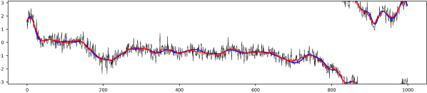
Figure 1: Ground truth (blue), noisy observation with $\kappa=10$ (black), and numerical solution (red) of the line graph signal of length $N=1000$ in Section VI-A. The $\mathbb{S}_{1}$-values are represented by their angles in $[-\pi,\pi)$.

TABLE I: The mean distance to the circle, computation time, and iteration numbers for the line graph signal in Section VI-A with $\kappa=10$. The recorded values are averages over 50 randomly generated ground truths.

	mean	time	iter.
PMM on (II-A)	$10^{-9}$	$2.10$	$201$
ADMM on (II-A)	$10^{-12}$	$1.83$	$182$
ADMM on (19)	$10^{-13}$	$1.77$	$181$

VI-A $\mathbb{S}_{1}$-Valued Data

We start with a synthetic, smooth signal $(\bm{x}_{n})_{n\in V}$ on the line graph. More precisely, we consider the circle-valued, one-dimensional signal in Figure 1. The synthetic noisy observation $(\bm{y}_{n})_{n\in V}$ are generated using the von Mises–Fisher distribution by

$$\bm{y}_{n}\sim\mathcal{N}_{\text{vMF}}(\bm{x}_{n},\kappa)\quad\text{for all}\quad n\in V,$$

where $\kappa>0$ is the so-called capacity. To denoise the generated measurements, we apply PMM ($\tau\coloneqq 0.1$, $\sigma\coloneqq(4\tau)^{-1}$) and ADMM ($\rho\coloneqq 3$) on the relaxed complex model (II-A) and compare these with ADMM ($\rho\coloneqq 3$) in Algorithm 14 for the simplified relaxed real model (19), where the regularization parameters are chosen as $w_{n}\coloneqq 1$ and $\lambda_{(n,m)}\coloneqq 25$. Starting all algorithms from zero, we observe convergence to the same limit, which is shown in Figure 1. To compare the convergence speed, we run all algorithms for 600 iterations and determine the time after which the objective remains in a small $\epsilon\coloneqq 10^{-5}$ neighbourhood around the limiting value. These times are recorded in Table I. For the relaxed complex model (II-A), ADMM shows a significant speed-up compared with PMM. Moreover, switching to our simplified relaxed real model gives an additional acceleration. Notice that the solution $(\tilde{\bm{x}}_{n})_{n\in V}$ of (19) fulfils $\lVert\tilde{\bm{x}}_{n}\rVert\leq 1$, since $\bm{Q}_{(n,m)}\succeq 0$ and thus

$$\det\Bigl{(}\begin{smallmatrix}\bm{I}&\tilde{\bm{x}}_{n}\\ \tilde{\bm{x}}_{n}^{\mathrm{T}}&1\end{smallmatrix}\Bigr{)}=1-\lVert\tilde{\bm{x}}_{n}\rVert^{2}\geq 0$$

for all $(n,m)\in E$. For the relaxed complex models, there holds an analogous observation. Determining the mean of $1-\lVert\tilde{\bm{x}}_{n}\rVert$ over $n\in V$ as well as of $1-\lvert x_{n}\rvert$ for the numerical real and complex solutions, see Table I, we observe convergence the circle, i.e. the numerical solutions solve the original (unrelaxed) problem (8).

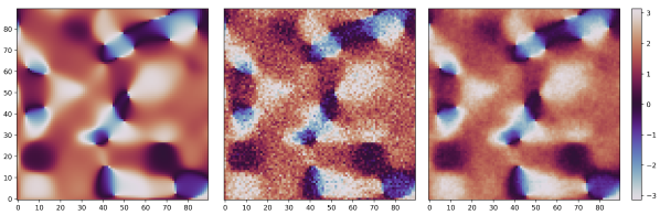
Figure 2: Ground truth (left), noisy observation with $\kappa=20$ (middle), and numerical solution (right) of the image graph signal on $90\times 90$ pixels in Section VI-A. The colour map corresponds to the angles of the $\mathbb{S}_{1}$-values.

TABLE II: The mean distance to the circle, computation time, and iteration numbers for the image graph signal in Section VI-A with $\kappa=20$. The recorded values are averages over 50 randomly generated ground truths.

	mean	time	iter.
PMM on (II-A)	$10^{-4}$	$747.18$	$5536$
ADMM on (II-A)	$10^{-4}$	$389.01$	$2457$
ADMM on (19)	$10^{-4}$	$301.08$	$1943$

For $\mathbb{S}_{1}$-valued images, the (image) graph $G$ consists of the image pixels, which are connected to their vertical and horizontal neighbours. As before, we generate synthetic observation using the von Mises–Fisher distribution. The synthetic observations are denoised using PMM ($\tau\coloneqq 0.1$, $\sigma\coloneqq(8\tau)^{-1}$) and ADMM ($\rho\coloneqq 20$) on the relaxed complex model (II-A) as well as ADMM ($\rho\coloneqq 20$) on the simplified relaxed real model (19), where the regularization parameters are chosen as $w_{n}\coloneqq 1$ and $\lambda_{(n,m)}\coloneqq 1$. The generated data together with its denoised version, which nearly coincides for all three methods, are shown in Figure 2. Different from the one-dimensional setting, all methods show much slower numerical convergence. The times after which the objective stays in an $\epsilon\coloneqq 10^{-4}$ neighborhood around the limiting value after 6000 iterations is shown in Table II. Similarly, the convergence of $\bm{x}_{n}$ to $\mathbb{S}_{1}$ and $x_{n}$ to $\mathbb{S}_{\mathbb{C}}$ is slowed down but can be observed for most pixels after the final iteration. This behaviour has also been observed in [27] and transfers to our simplified relaxed real model. It seems that this drawback only occurs for circle-valued images. The benefit of ADMM and our simplified relaxed real model with respect to the computation time are clearly visible.

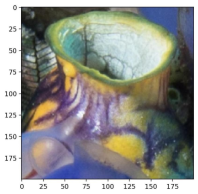
Figure 3: Ground truth of size $200\times 200$ for the colour denoising in Section VI-B.

VI-B Denoising Colour Values

Sphere-valued data naturally occur as colour information of colour images. For instance, the hue of the HSV (hue, saturation, value) colour model is $\mathbb{S}_{1}$-valued, and the chromaticity of the CB (chromaticity, brightness) colour model is $\mathbb{S}_{2}$-valued, see [38, § 1.1]. Identifying the circle $\mathbb{S}_{1}=\{(\cos\alpha,\sin\alpha)^{\mathrm{T}}:\alpha\in[0,2\pi)\}$ with the angle $\alpha\in[0,2\pi)$, the hue starts with red at $0$, goes over green at $2\pi/3$ and blue at $4\pi/3$, and return to red at $2\pi$. The chromaticity is the normalized colour vector of the RGB (red, green, blue) model. For the numerical simulations, we take the hue and the chromaticity of the colour image in Figure 3, perturb the colour values according to the von Mises–Fisher distribution, and apply Algorithm 14 based on the simplified real model for denoising. The results are shown in Figure 4 and 5. Visually, most of the noise is removed.

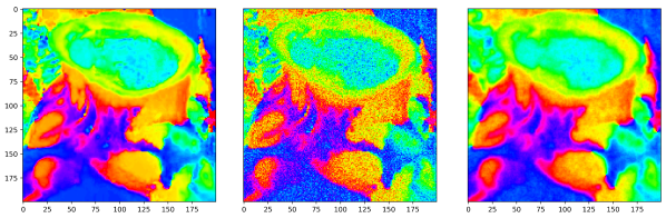
Figure 4: Ground truth (left), noisy observation with $\kappa=10$ (middle), and denoised version (right) of the hue experiment in Section VI-B with respect to Figure 3. ADMM has been employed with $w_{n}\coloneqq 1$, $\lambda_{(n,m)}\coloneqq 2$, and $\rho\coloneqq 20$.

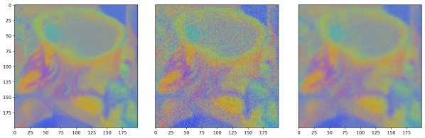
Figure 5: Ground truth (left), noisy observation with $\kappa=100$ (middle), and denoised version (right) of the chromaticity experiment in Section VI-B with respect to Figure 3. ADMM has been employed with $w_{n}\coloneqq 1$, $\lambda_{(n,m)}\coloneqq 3$, and $\rho\coloneqq 3$.

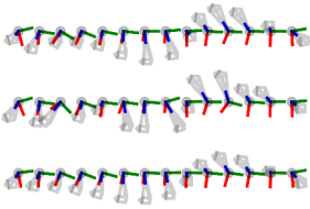
Figure 6: Ground truth (top), noisy observation with $\kappa_{1}\coloneqq 30$ and $\kappa_{2}\coloneqq 15$ (middle), and denoised version (bottom) of the ${\mathrm{SO}}(3)$-valued signal on the line graph in Section VI-C. The rotations are visualized by operating on a 3d object. The red, green, and blue lines indicate the rotated unit vectors. The entire signal has a length of $N\coloneqq 1000$, where only the rotations at $n=1,11,21,31,\dots$ are visualized. The parameters have been $w_{n}\coloneqq 1$, $\lambda_{(n,m)}\coloneqq 50$, and $\rho\coloneqq 3$.

VI-C ${\mathrm{SO}}(3)$-Valued Data

As discussed in Section IV, we want to employ Algorithm 14 to denoise 3d rotation data on line and image graphs. Starting from a smooth ${\mathrm{SO}}(3)$-valued signal $(\bm{R}_{n})_{n\in V}$ corresponding to the rotation axes $\bm{v}_{n}\in\mathbb{S}_{2}$ and rotation angles $\alpha_{n}\in\mathbb{S}_{1}$, i.e. $\bm{R}_{n}=\bm{R}(\bm{v}_{n},\alpha_{n})$, we generate disturbed rotation axes and angles with respect to the von Mises–Fisher distributions on $\mathbb{S}_{2}$ and $\mathbb{S}_{1}$. More precisely, we sample

$$\bm{w}_{n}\sim\mathcal{N}_{\text{vMF}}(\bm{v}_{n},\kappa_{1})\quad\text{and}\quad\beta_{n}\sim\mathcal{N}_{\text{vMF}}(\alpha_{n},\kappa_{2}).$$

The synthetic observations are then given by $(\bm{S}_{n})_{n\in V}$ with $\bm{S}_{n}\coloneqq\bm{R}(\bm{w}_{n},\beta_{n})$. The aim is now to denoise the signal $(\bm{S}_{n})_{n\in V}$. For this, we use the double cover ${\mathrm{SO}}(3)\cong\mathbb{S}_{\mathbb{H}}/\{-1,1\}$ to represent the $3\times 3$ matrices $\bm{S}_{n}$ by their quaternion $q_{n}\coloneqq\pm q(\bm{w}_{n},\beta_{n})$, see (41). Starting with $q_{1}\coloneqq q(\bm{w}_{1},\beta_{1})$ the remaining signs of $q_{n}$ are here chosen such that $\Re[q_{n}\bar{q}_{m}]\geq 0$ for all $(n,m)\in E$. In this example, the original signal is smooth and the noise small enough such that the sign choice is well defined. Finally, Algorithm 14 is employed on the vector representations $\bm{q}_{n}\coloneqq(\Re[q_{n}],\Im_{\mathrm{i}}[q_{n}],\Im_{\mathrm{j}}[q_{n}],\Im_{\mathrm{k}}[q_{n}])^{\mathrm{T}}$. For the line graph, see Figure 6, ADMM takes 8.60 seconds (209 iterations) to converge. For the image graph, see Figure 7, ADMM needs 41.69 seconds (219 iterations) until convergence. In both cases, the mean of $1-\lVert\bm{q}_{n}\rVert$ over $n\in V$ reaches $10^{-9}$ after around 200 iterations. Hence, the computed numerical solutions are in fact solutions of the original unrelaxed problem.

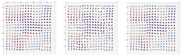
Figure 7: Ground truth (left), noisy observation with $\kappa_{1}\coloneqq 30$ and $\kappa_{2}\coloneqq 5$ (middle), and denoised version (right) of the ${\mathrm{SO}}(3)$-valued signal on the image graph in Section VI-C. The rotations are visualized by operating on a colored 3d cone. The entire signal consists of $90\times 90$ pixel, where only every third pixel from the 25th to the 75th pixel is visualized. The parameters have been $w_{n}\coloneqq 1$, $\lambda_{(n,m)}\coloneqq 1$, and $\rho\coloneqq 3$.

[Proof of Theorem 9]

Recall the identification of the quaternion $z\in\mathbb{H}$ with $\bm{z}\coloneqq(\Re[z],\Im_{\mathrm{i}}[z],\Im_{\mathrm{j}}[z],\Im_{\mathrm{k}}[z])\in\mathbb{R}^{4}$ such that $\lvert z\rvert=\lVert\bm{z}\rVert$. Moreover, each quaternion can be identified with the matrix

$$\bm{M}(z)\coloneqq\left[\begin{smallmatrix}\Re[z]&-\Im_{\mathrm{i}}[z]&-\Im_{\mathrm{j}}[z]&-\Im_{\mathrm{k}}[z]\\ \Im_{\mathrm{i}}[z]&\Re[z]&-\Im_{\mathrm{k}}[z]&\Im_{\mathrm{j}}[z]\\ \Im_{\mathrm{j}}[z]&\Im_{\mathrm{k}}[z]&\Re[z]&-\Im_{\mathrm{i}}[z]\\ \Im_{\mathrm{k}}[z]&-\Im_{\mathrm{j}}[z]&\Im_{\mathrm{i}}[z]&\Re[z]\end{smallmatrix}\right]\in\mathbb{R}^{4\times 4}.$$

In this way, the addition and multiplication of quaternions carries over to the addition and multiplication of the associated matrices. The matrix $P_{(n,m)}\in\mathbb{H}^{3\times 3}$ in (44) is positive semi-definite if and only if the real-valued representation

$$\bm{P}_{(n,m)}\coloneqq\left[\begin{smallmatrix}\bm{I}_{4}&\bm{M}(x_{n})&\bm{M}(x_{m})\\ \bm{M}(x_{n})^{\mathrm{T}}&\bm{I}_{4}&\bm{M}(r_{(n,m)})^{\mathrm{T}}\\ \bm{M}(x_{m})^{\mathrm{T}}&\bm{M}(r_{(n,m)})&\bm{I}_{4}\end{smallmatrix}\right]\in\mathbb{R}^{12\times 12}$$ (64)

is positive semi-definite. In order to establish the equality between quaternion model (IV) and the real-valued model in (38) for $d=4$, we compare the Schur complements of a permuted version of $\bm{P}_{(n,m)}$ and of $\bm{Q}_{(n,m)}$. First, we compute the Schur complement of $\bm{Q}_{m,n}$ in (47) with respect to $\bm{I}_{4}$, which is again given by

$$\bm{Q}_{(n,m)}/\bm{I}_{4}=\left[\begin{smallmatrix}1-\lvert\bm{x}_{n}\rvert^{2}&\bm{\ell}_{(n,m)}-\langle\bm{x}_{n},\bm{x}_{m}\rangle\\ \bm{\ell}_{(n,m)}-\langle\bm{x}_{n},\bm{x}_{m}\rangle&1-\lvert\bm{x}_{m}\rvert^{2}\end{smallmatrix}\right].$$

Second, we consider the matrix $\bm{P}_{(n,m)}$ whose details are given in Table IIIa. Permuting the columns and rows of $\bm{P}_{(n,m)}$ with respect to the permutation $(1,2,3,4,5,9,6,10,7,11,8,12)$, we obtain $\tilde{\bm{P}}_{(n,m)}$ in Table IIIb. Forming the Schur complement with respect to the upper left identity results in the block matrix $\tilde{\bm{P}}_{(n,m)}/\bm{I}_{4}$ in Table IIIc.

TABLE III: Reformulating $P_{(n,m)}$ by writing out its real-valued representation $\bm{P}_{(n,m)}$, permuting the columns/rows with respect to the permutation $(1,2,3,4,5,9,6,10,7,11,8,12)$, and calculating the Schur complement with respect to the upper left identity matrix.

$\left[\scalebox{0.8}{$\begin{array}[]{*{2}{cccc|}cccc}1&0&0&0&\Re[x_{n}]&-\Im_{\mathrm{i}}[x_{n}]&-\Im_{\mathrm{j}}[x_{n}]&-\Im_{\mathrm{k}}[x_{n}]&\Re[x_{m}]&-\Im_{\mathrm{i}}[x_{m}]&-\Im_{\mathrm{j}}[x_{m}]&-\Im_{\mathrm{k}}[x_{m}]\\ 0&1&0&0&\Im_{\mathrm{i}}[x_{n}]&\Re[x_{n}]&-\Im_{\mathrm{k}}[x_{n}]&\Im_{\mathrm{j}}[x_{n}]&\Im_{\mathrm{i}}[x_{m}]&\Re[x_{m}]&-\Im_{\mathrm{k}}[x_{m}]&\Im_{\mathrm{j}}[x_{m}]\\ 0&0&1&0&\Im_{\mathrm{j}}[x_{n}]&\Im_{\mathrm{k}}[x_{n}]&\Re[x_{n}]&-\Im_{\mathrm{i}}[x_{n}]&\Im_{\mathrm{j}}[x_{m}]&\Im_{\mathrm{k}}[x_{m}]&\Re[x_{m}]&-\Im_{\mathrm{i}}[x_{m}]\\ 0&0&0&1&\Im_{\mathrm{k}}[x_{n}]&-\Im_{\mathrm{j}}[x_{n}]&\Im_{\mathrm{i}}[x_{n}]&\Re[x_{n}]&\Im_{\mathrm{k}}[x_{m}]&-\Im_{\mathrm{j}}[x_{m}]&\Im_{\mathrm{i}}[x_{m}]&\Re[x_{m}]\\ \hline\cr\Re[x_{n}]&\Im_{\mathrm{i}}[x_{n}]&\Im_{\mathrm{j}}[x_{n}]&\Im_{\mathrm{k}}[x_{n}]&1&0&0&0&\Re[r_{(n,m)}]&\Im_{\mathrm{i}}[r_{(n,m)}]&\Im_{\mathrm{j}}[r_{(n,m)}]&\Im_{\mathrm{k}}[r_{(n,m)}]\\ -\Im_{\mathrm{i}}[x_{n}]&\Re[x_{n}]&\Im_{\mathrm{k}}[x_{n}]&-\Im_{\mathrm{j}}[x_{n}]&0&1&0&0&-\Im_{\mathrm{i}}[r_{(n,m)}]&\Re[r_{(n,m)}]&\Im_{\mathrm{k}}[r_{(n,m)}]&-\Im_{\mathrm{j}}[r_{(n,m)}]\\ -\Im_{\mathrm{j}}[x_{n}]&-\Im_{\mathrm{k}}[x_{n}]&\Re[x_{n}]&\Im_{\mathrm{i}}[x_{n}]&0&0&1&0&-\Im_{\mathrm{j}}[r_{(n,m)}]&-\Im_{\mathrm{k}}[r_{(n,m)}]&\Re[r_{(n,m)}]&\Im_{\mathrm{i}}[r_{(n,m)}]\\ -\Im_{\mathrm{k}}[x_{n}]&\Im_{\mathrm{j}}[x_{n}]&-\Im_{\mathrm{i}}[x_{n}]&\Re[x_{n}]&0&0&0&1&-\Im_{\mathrm{k}}[r_{(n,m)}]&\Im_{\mathrm{j}}[r_{(n,m)}]&-\Im_{\mathrm{i}}[r_{(n,m)}]&\Re[r_{(n,m)}]\\ \hline\cr\Re[x_{m}]&\Im_{\mathrm{i}}[x_{m}]&\Im_{\mathrm{j}}[x_{m}]&\Im_{\mathrm{k}}[x_{m}]&\Re[r_{(n,m)}]&-\Im_{\mathrm{i}}[r_{(n,m)}]&-\Im_{\mathrm{j}}[r_{(n,m)}]&-\Im_{\mathrm{k}}[r_{(n,m)}]&1&0&0&0\\ -\Im_{\mathrm{i}}[x_{m}]&\Re[x_{m}]&\Im_{\mathrm{k}}[x_{m}]&-\Im_{\mathrm{j}}[x_{m}]&\Im_{\mathrm{i}}[r_{(n,m)}]&\Re[r_{(n,m)}]&-\Im_{\mathrm{k}}[r_{(n,m)}]&\Im_{\mathrm{j}}[r_{(n,m)}]&0&1&0&0\\ -\Im_{\mathrm{j}}[x_{m}]&-\Im_{\mathrm{k}}[x_{m}]&\Re[x_{m}]&\Im_{\mathrm{i}}[x_{m}]&\Im_{\mathrm{j}}[r_{(n,m)}]&\Im_{\mathrm{k}}[r_{(n,m)}]&\Re[r_{(n,m)}]&-\Im_{\mathrm{i}}[r_{(n,m)}]&0&0&1&0\\ -\Im_{\mathrm{k}}[x_{m}]&\Im_{\mathrm{j}}[x_{m}]&-\Im_{\mathrm{i}}[x_{m}]&\Re[x_{m}]&\Im_{\mathrm{k}}[r_{(n,m)}]&-\Im_{\mathrm{j}}[r_{(n,m)}]&\Im_{\mathrm{i}}[r_{(n,m)}]&\Re[r_{(n,m)}]&0&0&0&1\end{array}$}\right]$

(a) Real-valued representation $\bm{P}_{(n,m)}$ of $P_{(n,m)}$.

$\left[\scalebox{0.8}{$\begin{array}[]{cccc|*{8}{c}}1&0&0&0&\Re[x_{n}]&\Re[x_{m}]&-\Im_{\mathrm{i}}[x_{n}]&-\Im_{\mathrm{i}}[x_{m}]&-\Im_{\mathrm{j}}[x_{n}]&-\Im_{\mathrm{j}}[x_{m}]&-\Im_{\mathrm{k}}[x_{n}]&-\Im_{\mathrm{k}}[x_{m}]\\ 0&1&0&0&\Im_{\mathrm{i}}[x_{n}]&\Im_{\mathrm{i}}[x_{m}]&\Re[x_{n}]&\Re[x_{m}]&-\Im_{\mathrm{k}}[x_{n}]&-\Im_{\mathrm{k}}[x_{m}]&\Im_{\mathrm{j}}[x_{n}]&\Im_{\mathrm{j}}[x_{m}]\\ 0&0&1&0&\Im_{\mathrm{j}}[x_{n}]&\Im_{\mathrm{j}}[x_{m}]&\Im_{\mathrm{k}}[x_{n}]&\Im_{\mathrm{k}}[x_{m}]&\Re[x_{n}]&\Re[x_{m}]&-\Im_{\mathrm{i}}[x_{n}]&-\Im_{\mathrm{i}}[x_{m}]\\ 0&0&0&1&\Im_{\mathrm{k}}[x_{n}]&\Im_{\mathrm{k}}[x_{m}]&-\Im_{\mathrm{j}}[x_{n}]&-\Im_{\mathrm{j}}[x_{m}]&\Im_{\mathrm{i}}[x_{n}]&\Im_{\mathrm{i}}[x_{m}]&\Re[x_{n}]&\Re[x_{m}]\\ \hline\cr\Re[x_{n}]&\Im_{\mathrm{i}}[x_{n}]&\Im_{\mathrm{j}}[x_{n}]&\Im_{\mathrm{k}}[x_{n}]&1&\Re[r_{(n,m)}]&0&\Im_{\mathrm{i}}[r_{(n,m)}]&0&\Im_{\mathrm{j}}[r_{(n,m)}]&0&\Im_{\mathrm{k}}[r_{(n,m)}]\\ \Re[x_{m}]&\Im_{\mathrm{i}}[x_{m}]&\Im_{\mathrm{j}}[x_{m}]&\Im_{\mathrm{k}}[x_{m}]&\Re[r_{(n,m)}]&1&-\Im_{\mathrm{i}}[r_{(n,m)}]&0&-\Im_{\mathrm{j}}[r_{(n,m)}]&0&-\Im_{\mathrm{k}}[r_{(n,m)}]&0\\ -\Im_{\mathrm{i}}[x_{n}]&\Re[x_{n}]&\Im_{\mathrm{k}}[x_{n}]&-\Im_{\mathrm{j}}[x_{n}]&0&-\Im_{\mathrm{i}}[r_{(n,m)}]&1&\Re[r_{(n,m)}]&0&\Im_{\mathrm{k}}[r_{(n,m)}]&0&-\Im_{\mathrm{j}}[r_{(n,m)}]\\ -\Im_{\mathrm{i}}[x_{m}]&\Re[x_{m}]&\Im_{\mathrm{k}}[x_{m}]&-\Im_{\mathrm{j}}[x_{m}]&\Im_{\mathrm{i}}[r_{(n,m)}]&0&\Re[r_{(n,m)}]&1&-\Im_{\mathrm{k}}[r_{(n,m)}]&0&\Im_{\mathrm{j}}[r_{(n,m)}]&0\\ -\Im_{\mathrm{j}}[x_{n}]&-\Im_{\mathrm{k}}[x_{n}]&\Re[x_{n}]&\Im_{\mathrm{i}}[x_{n}]&0&-\Im_{\mathrm{j}}[r_{(n,m)}]&0&-\Im_{\mathrm{k}}[r_{(n,m)}]&1&\Re[r_{(n,m)}]&0&\Im_{\mathrm{i}}[r_{(n,m)}]\\ -\Im_{\mathrm{j}}[x_{m}]&-\Im_{\mathrm{k}}[x_{m}]&\Re[x_{m}]&\Im_{\mathrm{i}}[x_{m}]&\Im_{\mathrm{j}}[r_{(n,m)}]&0&\Im_{\mathrm{k}}[r_{(n,m)}]&0&\Re[r_{(n,m)}]&1&-\Im_{\mathrm{i}}[r_{(n,m)}]&0\\ -\Im_{\mathrm{k}}[x_{n}]&\Im_{\mathrm{j}}[x_{n}]&-\Im_{\mathrm{i}}[x_{n}]&\Re[x_{n}]&0&-\Im_{\mathrm{k}}[r_{(n,m)}]&0&\Im_{\mathrm{j}}[r_{(n,m)}]&0&-\Im_{\mathrm{i}}[r_{(n,m)}]&1&\Re[r_{(n,m)}]\\ -\Im_{\mathrm{k}}[x_{m}]&\Im_{\mathrm{j}}[x_{m}]&-\Im_{\mathrm{i}}[x_{m}]&\Re[x_{m}]&\Im_{\mathrm{k}}[r_{(n,m)}]&0&-\Im_{\mathrm{j}}[r_{(n,m)}]&0&\Im_{\mathrm{i}}[r_{(n,m)}]&0&\Re[r_{(n,m)}]&1\end{array}$}\right]$

(b) Permuted matrix $\tilde{\bm{P}}_{(n,m)}$ build from $\bm{P}_{(n,m)}$.

$\left[\scalebox{0.6}{$\begin{array}[]{*{3}{cc|}cc}1-\lvert x_{n}\rvert^{2}&\Re[r_{(n,m)}]-\Re[\bar{x}_{m}x_{n}]&0&\Im_{\mathrm{i}}[r_{(n,m)}]-\Im_{\mathrm{i}}[\bar{x}_{m}x_{n}]&0&\Im_{\mathrm{j}}[r_{(n,m)}]-\Im_{\mathrm{j}}[\bar{x}_{m}x_{n}]&0&\Im_{\mathrm{k}}[r_{(n,m)}]-\Im_{\mathrm{k}}[\bar{x}_{m}x_{n}]\\ \Re[r_{(n,m)}]-\Re[\bar{x}_{m}x_{n}]&1-\lvert x_{m}\rvert^{2}&-\Im_{\mathrm{i}}[r_{(n,m)}]+\Im_{\mathrm{i}}[\bar{x}_{m}x_{n}]&0&-\Im_{\mathrm{j}}[r_{(n,m)}]+\Im_{\mathrm{j}}[\bar{x}_{m}x_{n}]&0&-\Im_{\mathrm{k}}[r_{(n,m)}]+\Im_{\mathrm{k}}[\bar{x}_{m}x_{n}]&0\\ \hline\cr 0&-\Im_{\mathrm{i}}[r_{(n,m)}]+\Im_{\mathrm{i}}[\bar{x}_{m}x_{n}]&1-\lvert x_{n}\rvert^{2}&\Re[r_{(n,m)}]-\Re[\bar{x}_{m}x_{n}]&0&\Im_{\mathrm{k}}[r_{(n,m)}]-\Im_{\mathrm{k}}[\bar{x}_{m}x_{n}]&0&-\Im_{\mathrm{j}}[r_{(n,m)}]+\Im_{\mathrm{j}}[\bar{x}_{m}x_{n}]\\ \Im_{\mathrm{i}}[r_{(n,m)}]-\Im_{\mathrm{i}}[\bar{x}_{m}x_{n}]&0&\Re[r_{(n,m)}]-\Re[\bar{x}_{m}x_{n}]&1-\lvert x_{m}\rvert^{2}&-\Im_{\mathrm{k}}[r_{(n,m)}]+\Im_{\mathrm{k}}[\bar{x}_{m}x_{n}]&0&\Im_{\mathrm{j}}[r_{(n,m)}]-\Im_{\mathrm{j}}[\bar{x}_{m}x_{n}]&0\\ \hline\cr 0&-\Im_{\mathrm{j}}[r_{(n,m)}]+\Im_{\mathrm{j}}[\bar{x}_{m}x_{n}]&0&-\Im_{\mathrm{k}}[r_{(n,m)}]+\Im_{\mathrm{k}}[\bar{x}_{m}x_{n}]&1-\lvert x_{n}\rvert^{2}&\Re[r_{(n,m)}]-\Re[\bar{x}_{m}x_{n}]&0&\Im_{\mathrm{i}}[r_{(n,m)}]-\Im_{\mathrm{i}}[\bar{x}_{m}x_{n}]\\ \Im_{\mathrm{j}}[r_{(n,m)}]-\Im_{\mathrm{j}}[\bar{x}_{m}x_{n}]&0&\Im_{\mathrm{k}}[r_{(n,m)}]-\Im_{\mathrm{k}}[\bar{x}_{m}x_{n}]&0&\Re[r_{(n,m)}]-\Re[\bar{x}_{m}x_{n}]&1-\lvert x_{m}\rvert^{2}&-\Im_{\mathrm{i}}[r_{(n,m)}]+\Im_{\mathrm{i}}[\bar{x}_{m}x_{n}]&0\\ \hline\cr 0&-\Im_{\mathrm{k}}[r_{(n,m)}]+\Im_{\mathrm{k}}[\bar{x}_{m}x_{n}]&0&\Im_{\mathrm{j}}[r_{(n,m)}]-\Im_{\mathrm{j}}[\bar{x}_{m}x_{n}]&0&-\Im_{\mathrm{i}}[r_{(n,m)}]+\Im_{\mathrm{i}}[\bar{x}_{m}x_{n}]&1-\lvert x_{n}\rvert^{2}&\Re[r_{(n,m)}]-\Re[\bar{x}_{m}x_{n}]\\ \Im_{\mathrm{k}}[r_{(n,m)}]-\Im_{\mathrm{k}}[\bar{x}_{m}x_{n}]&0&-\Im_{\mathrm{j}}[r_{(n,m)}]+\Im_{\mathrm{j}}[\bar{x}_{m}x_{n}]&0&\Im_{\mathrm{i}}[r_{(n,m)}]-\Im_{\mathrm{i}}[\bar{x}_{m}x_{n}]&0&\Re[r_{(n,m)}]-\Re[\bar{x}_{m}x_{n}]&1-\lvert x_{m}\rvert^{2}\end{array}$}\right]$

(c) Schur complement $\tilde{\bm{P}}_{(n,m)}/\bm{I}_{4}$ containing $\bm{Q}_{(n,m)}/\bm{I}_{4}$ on the diagonal.

Comparing the Schur complements $\bm{Q}_{(n,m)}/\bm{I}_{4}$ and $\tilde{\bm{P}}_{(n,m)}/\bm{I}_{4}$ and using $\Re[\bar{x}_{m}x_{n}]=\langle\bm{x}_{m},\bm{x}_{n}\rangle$, we obtain the following: if $(\hat{x},\hat{r})$ solves (IV), then $(\hat{\bm{x}},\hat{\bm{\ell}})$ with $\hat{\bm{\ell}}_{(n,m)}\coloneqq\Re[\hat{r}_{(n,m)})]$ is a feasible point of (38). Moreover, it holds $\mathcal{K}(\hat{\bm{x}},\hat{\bm{\ell}})=\mathcal{J}(\hat{x},\hat{r})$. Conversely, if $(\tilde{\bm{x}},\tilde{\bm{\ell}})$ solves (38), then $(\tilde{x},\tilde{r})$ with $\tilde{r}$ defined in the assertion is a feasible point of (IV)—all off-diagonal blocks of $\tilde{\bm{P}}_{(n,m)}/\bm{I}_{4}$ become zero—and again $\mathcal{K}(\tilde{\bm{x}},\tilde{\bm{\ell}})=\mathcal{J}(\tilde{x},\tilde{r})$. Then, taking the minimizing property into account, we conclude

$$\mathcal{K}(\tilde{\bm{x}},\tilde{\bm{\ell}})\leq\mathcal{K}(\hat{\bm{x}},\hat{\bm{\ell}})=\mathcal{J}(\hat{x},\hat{r})\leq\mathcal{J}(\tilde{x},\tilde{r})=\mathcal{K}(\tilde{\bm{x}},\tilde{\bm{\ell}})$$

which is only possible if all values coincides. This yields the assertion. $\square$

References

- [1] R. Bürgmann, P. A. Rosen, and E. J. Fielding, “Synthetic aperture radar interferometry to measure earth’s surface topography and its deformation,” Annu. Rev. Earth Planet Sci., vol. 28, no. 1, pp. 169–209, 2000.
- [2] C.-A. Deledalle, L. Denis, and F. Tupin, “NL-InSAR: Nonlocal interferogram estimation,” IEEE Trans. Geosci. Remote Sens., vol. 49, no. 4, pp. 1441–1452, 2011.
- [3] P. A. Rosen, S. Hensley, I. R. Joughin, F. K. Li, S. N. Madsen, E. Rodriguez, and R. M. Goldstein, “Synthetic aperture radar interferometry,” Proc. IEEE, vol. 88, no. 3, pp. 333–382, 2000.
- [4] M. Nikolova and G. Steidl, “Fast hue and range preserving histogram specification: theory and new algorithms for color image enhancement,” IEEE Trans. Image Process., vol. 23, no. 9, pp. 4087–4100, 2014.
- [5] T. Lan, D. Erdogmus, S. J. Hayflick, and J. U. Szumowski, “Phase unwrapping and background correction in MRI,” in Proceedings MLSP ’08’, 2008, pp. 239–243, IEEE Workshop on Machine Learning for Signal Processing, 16-19 October 2008, Cancun, Mexico.
- [6] Y. Sowa, A. D. Rowe, M. C. Leake, T. Yakushi, M. Homma, A. Ishijima, and R. M. Berry, “Direct observation of steps in rotation of the bacterial flagellar motor,” Nature, vol. 437, pp. 916–919, 2005.
- [7] J. Cremers and I. Klugkist, “One direction? A tutorial for circular data analysis using R with examples in cognitive psychology,” Front. Psychol., vol. 9, no. 2040, 2018.
- [8] B. L. Adams, S. I. Wright, and K. Kunze, “Orientation imaging: the emergence of a new microscopy,” Metall. Mater. Trans. A Phys. Metall. Mater. Sci., vol. 24, pp. 819–831, 1993.
- [9] R. Kimmel and N. Sochen, “Orientation diffusion or how to comb a porcupine,” J. Vis. Commun. Image. Represent., vol. 13, no. 1, pp. 238–248, 2002.
- [10] L. A. Vese and S. J. Osher, “Numerical methods for p-harmonic flows and applications to image processing,” SIAM J. Numer. Anal., vol. 40, no. 6, pp. 2085–2104, 2002.
- [11] T. Batard and M. Bertalmio, “A geometric model of brightness perception and its application to color image correction,” J. Math. Imaging Vis., vol. 60, no. 6, pp. 849–881, 2018.
- [12] J. Persch, F. Pierre, and G. Steidl, “Exemplar-based face colorization using image morphing,” J. Imaging, vol. 3, no. 4, p. 48, 2017.
- [13] M. H. Quang, S. H. Kang, and T. M. Le, “Image and video colorization using vector-valued reproducing kernel Hilbert spaces,” J. Math. Imaging Vis., vol. 37, pp. 49–65, 2010.
- [14] F. Bachmann, R. Hielscher, and H. Schaeben, “Grain detection from 2d and 3d EBSD data—specification of the MTEX algorithm,” Ultramicroscopy, vol. 111, no. 12, pp. 1720–1733, 2011.
- [15] F. Bachmann, R. Hielscher, P. E. Jupp, W. Pantleon, H. Schaeben, and E. Wegert, “Inferential statistics of electron backscatter diffraction data from within individual crystalline grains,” J. Appl. Crystallogr., vol. 43, pp. 1338–1355, 2010.
- [16] M. Gräf, S. Neumayer, R. Hielscher, G. Steidl, M. Liesegang, and T. Beck, “An optical flow model in electron backscatter diffraction,” SIAM J. Imaging Sci., vol. 15, no. 1, pp. 228–260, 2022.
- [17] D. Cremers and E. Strekalovskiy, “Total cyclic variation and generalizations,” J. Math. Imaging Vis., vol. 47, no. 3, pp. 258–277, 2013.
- [18] E. Strekalovskiy and D. Cremers, “Total variation for cyclic structures: convex relaxation and efficient minimization,” in Proceedings CVPR ’11, 2011, pp. 1905–1911, IEEE Conference on Computer Vision and Pattern Recognition, 20-25 June 2011, Colorado Springs, USA.
- [19] J. Lellmann, E. Strekalovskiy, S. Koetter, and D. Cremers, “Total variation regularization for functions with values in a manifold,” in Proceedings ICCV ’13, 2013, pp. 2944–2951, IEEE International Conference on Computer Vision, 1–8 December 2013, Sydney, Australia.
- [20] M. Bačák, R. Bergmann, G. Steidl, and A. Weinmann, “A second order non-smooth variational model for restoring manifold-valued images,” SIAM J. Sci. Comput., vol. 38, no. 1, pp. A567–A597, 2016.
- [21] A. Weinmann, L. Demaret, and M. Storath, “Total variation regularization for manifold-valued data,” SIAM J. Imaging Sci., vol. 7, no. 4, pp. 2226–2257, 2014.
- [22] R. Bergmann, R. H. Chan, R. Hielscher, J. Persch, and G. Steidl, “Restoration of manifold-valued images by half-quadratic minimization,” Inverse Probl. Imaging, vol. 10, no. 2, pp. 281–304, 2016.
- [23] P. Grohs and M. Sprecher, “Total variation regularization on Riemannian manifolds by iteratively reweighted minimization,” Inf. Inference, vol. 5, no. 4, pp. 353–378, 2016.
- [24] X. Pennec, “Intrinsic statistics on Riemannian manifolds: basic tools for geometric measurements,” SIAM J. Imaging Sci., vol. 25, pp. 127–154, 2006.
- [25] F. Laus, M. Nikolova, J. Persch, and G. Steidl, “A nonlocal denoising algorithm for manifold-valued images using second order statistics,” SIAM J. Imaging Sci., vol. 10, no. 1, pp. 416–448, 2017.
- [26] R. Bergmann, F. Laus, J. Persch, and G. Steidl, “Recent advances in denoising of manifold-valued images,” in Handbook of Numerical Analysis, R. Kimmel and X.-C. Tai, Eds. Elsevier, 2019, vol. 20, pp. 553–578.
- [27] L. Condat, “Tikhonov regularization of circle-valued signals,” IEEE Trans. Signal Process., vol. 70, pp. 2775–2782, 2022.
- [28] ——, “Tikhonov regularization of sphere-valued signals,” 2022, arxiv:2207.12330.
- [29] R. A. Horn and C. R. Johnson, Matrix Analysis, 2nd ed. Cambridge: Cambridge University Press, 2012.
- [30] M. Gräf, “A unified approach to scattered data approximation on and ,” Adv. Comput. Math., vol. 37, pp. 379–392, 2012.
- [31] G. E. Bredon, Topology and Geometry, ser. Graduate Texts in Mathematics. New York: Springer, 1993, no. 139.
- [32] F. Zhang, “Quaternions and matrices of quaternions,” Linear Algebra Appl., vol. 251, pp. 21–57, 1997.
- [33] D. Huynh, “Metrics for 3d rotations: Comparison and analysis,” SIAM J. Imaging Sci., vol. 35, pp. 155–164, 10 2009.
- [34] S. Boyd, N. Parikh, E. Chu, B. Peleato, and J. Eckstein, “Distributed optimization and statistical learning via the alternating direction method of multipliers,” Found. Trends Mach. Learn., vol. 3, no. 1, pp. 1–122, 2010.
- [35] N. Parikh and S. P. Boyd, “Proximal algorithms,” Found. Trends Optim., vol. 1, pp. 127–239, 2013.
- [36] M. Burger, A. Sawatzky, and G. Steidl, “First order algorithms in variational image processing,” in Splitting methods in communication, imaging, science, and engineering, ser. Sci. Comput., R. Glowinski, S. Osher, and W. Yin, Eds. Cham: Springer, 2017, pp. 345–407.
- [37] H. H. Bauschke and P. L. Combettes, Convex analysis and monotone operator theory in Hilbert spaces, ser. CMS Books in Mathematics/Ouvrages de Mathématiques de la SMC. New York: Springer, 2011.
- [38] T. Chan, S. Kang, and J. Shen, “Total variation denoising and enhancement of color images based on the CB and HSV color models,” J. Vis. Commun. Image Represent., vol. 12, no. 4, pp. 422–435, 2001.