Studentising non-parametric correlation estimators

Abstract

Studentisation upon rank-based linear estimators is generally considered an unnecessary topic, due to the domain restriction upon $S_{n}$, which exhibits constant variance. This assertion is functionally inconsistent with general analytic practice though. We introduce a general unbiased and minimum variance estimator upon the Beta-Binomially distributed Kemeny Hilbert space, which allows for permutation ties to exist and be uniquely measured. As individual permutation samples now exhibit unique random variance, a sample dependent variance estimator must now be introduced into the linear model. We derive and prove the Slutsky conditions to enable $t_{\nu}$-distributed Wald test statistics to be constructed, while stably exhibiting Gauss-Markov properties upon finite samples. Simulations demonstrate convergent decisions upon the two orthonormal Slutsky corrected Wald test statistics, verifying the projective geometric duality which exists upon the affine-linear Kemeny metric.

The original conceptualisation of the Studentisation procedure developed due to the observation of incomplete information with respect to the $\ell_{2}$-norm’s abelian Hilbert space. [4] chose to consider the problem wherein the variability of the normal distribution’s linear distances were unknown, and merely estimable upon an acquired sample. This reduces the total amount of given information presumed to exist within the abelian function space, resulting in the $t$-test statistics, which asymptotically wrt $n$ converge to the unit normal distribution under the null hypothesis $H_{0}$, when the degrees of freedom are taken to be the population, $\nu\to\infty^{+}$. Within the non-parametric abelian function domain space $S_{n}$, the symmetric group of order $n$ however, the population variance of $n$ permutations without ties are of fixed cardinality $|n!|$ and known fixed variance. The sole free parameter over the population of permutations for any fixed $n$ is then the distance of the observed vector from the population’s expectation, resulting in conventional the Wald $z$-test [1].

Hurley (2023a) introduced a geometric dual Hilbert metric, parallel to the conventional Frobenius norm, upon the [2] original metric distance function, which we recognise to be Beta-Binomially distributed. This allowed us to expand the so-called ‘non-parametric’ population set space, satisfying for any $n$ the Borel-Cantelli lemma (1.2) and establishes the existence of two Gauss-Markov estimators upon a sample of $n$ elements selected uniformly from the extended real line, $\mathcal{M}_{n}$. In this work, we use $n\in\mathbb{N}^{+}$ to reflect a local finite sample of observed elements, and the index $m\in\mathcal{M}_{n}\to\infty^{+}$ to denote a particular permutation within the space of observable permutations upon the sample, and its convergence to the population. However, it should be immediately noted that the local individual variances of the set $m\in\mathcal{M}_{n}$ are no longer fixed and constant, but are instead only restricted to be always finite and positive upon the observed sample.

Under these conditions, the event probability of a common uniform selection of random variables, for which the probability of observation upon $\mathcal{M}_{n}$ events are observed only once, is distinctly unlikely. This compromises the established variability of the population and the corresponding unique probability mapping, as said variability of the expected distances is a direct function of the observed sample elements, thereby resulting in a smaller expected variance than reasonable. Correspondingly, this would result in a standard Type I error scenario, wherein the over-powered local partial Wald tests bias inferences obtained upon the sample. We therefore derive a novel resolution to provide an analytic solution to the problem of Studentisation of partial Wald test statistics upon finite samples for generalisations of the non-parametric correlation coefficients, for a population termed $\mathcal{M}^{\ast}_{n}$.

1 Wald tests for non-parametric samples with unknown variances

We consider the problem of two independently sampled random variables upon the extended real line $(X^{n\times 1},Y^{n\times 1})\in\overline{\mathbb{R}},n\in\mathbb{N}^{+}.$ Assume as given that these two random variables of length $n$ exists a population of $m\in\mathcal{M}_{n}$ distinct permutations, whose distances are measured upon the Kemeny metric. The Kemeny metric is almost surely finite and converges for all $n$. Let it be immediately noted that the expectations of both random variables are not required to be finite upon the $\ell_{2}$-norm, and therefore the abelian $\ell_{2}$ norm function space upon the random variables is degenerate. However, for each observed random variable, there exists a corresponding population of finite permutations $\mathcal{M}_{n}$ upon which each element may be mapped, and a corresponding Frobenius basis space $(X_{\ast}^{n\times 1},Y_{\ast}^{n\times 1})$, for all $n$. These properties satisfy the Borel-Cantelli lemma for the Kemeny norm space. Let it also be noted that $E(U(\mathcal{M}_{n}))=0$, the expectation upon the population of distances for all $n$, is an unbiased estimator, and also that $E(X_{\ast})=E(Y_{\ast})=0.$ Both norm-spaces are therefore are unbiased location estimators, as are all affine-linear functions thereupon.

The selection event of a random variable permutation $m_{l}\in\mathcal{M}_{n}$ was originally assumed to be a unique occurrence under the Borel-Cantelli lemma, in that once it was observed, the space of valid observations upon a second variable was strictly decremented by $1$ for $l=1\,\ldots,n^{n}-n$ random variables. Therefore, upon $\mathcal{M}_{2}$, which contains two non-degenerate permutations, to construct the partial Wald $z$ test with known population variance, there are only two valid permutation selections. Once one element $m_{1}$ is observed, the second element $m_{2}$ occurs with known probability 1. However, consider the set should the probability of selection be instead sample dependent, rather than fixed before observation of the sample.

Under this conditional selection, the probability of the first element arising is $\tfrac{1}{2^{2}-2}$, yet the second also results in a probability of selection of $m_{2}$ remains unchanged to the first, rather than determinate. Thus, $m\to\infty^{+}\equiv m\to n^{n}-n$ if and only if the cardinality of the population is known and fixed à priori, and the probability of re-selection of the same common event is therefore 0. Assuming uniform sampling upon a population where this is not true, and the population neighbourhood of distances $U(\mathcal{M}_{n})$ is not validly defined upon only $n^{n}-n$ measures although the strictly sub-Gaussian support is still valid. If the variability of the distances increases, denoting a greater chance of larger distances being obtained, it would follow that Slutsky’s theorem would necessarily apply. A similar problem was first addressed by [4]. It should be noted that upon the domain $S_{n}$, this problem is strictly unobservable, and therefore $S_{n}\subset\mathcal{M}_{n},$ and for unknown population cardinality for any $n$, the studentification procedure we develop is strictly necessary upon the domain of $\mathcal{M}_{n}$ without further axiomatic assertions. The problem of ties and non-constant known variance upon $S_{n}$ was traditionally otherwise handled by the birthday paradox upon the presumption of continuous random finite variables, which minimised the probability of ties occurring. As the Kemeny abelian function space is a continuous Haar measure, the existence of a corresponding cumulative distribution function space under the continuous mapping theorem is strictly valid, and a corresponding $X^{n\times p}_{j},j=1,\ldots,p$ may be observed without restriction, subject only to the existence of linear orderability upon independently sampled elements wrt $n$. Let it be noted that upon the asymptotic population wrt $n\to\infty^{+}$, the Borel-Cantelli lemma still guarantees convergence, as $\lim_{n\to\infty^{2}}E(|\langle{X^{n\times 1},Y^{n\times 1}\rangle}|)<\infty^{2}.$

We first provide the Kemeny distance function, which is an unbiased Gauss-Markov estimator of the permutation distance upon the observed vector $X$ and a corresponding paired target $Y$. Without loss of generality, consider $Y=\mu^{1}$ a fixed permutation element within $\mathcal{M}_{n}$. Between these two extended real vectors which arise independently and identically, but which do not require identical distributions, the numerators of the requisite Wald test statistics may be defined using equation 1a.

$$d_{\kappa}(X,Y)=\frac{n^{2}-n}{2}+\sum_{k,l=1}^{n}\kappa_{kl}(X)\odot\kappa_{kl}^{\intercal}(Y),~{}k,l=1,\ldots,n.$$ (1a)

Note that $\odot$ here denotes the Hadamard, element-wise, product, and that any affine-linear function upon this distance function is both an unbiased and minimum variance estimator, for any sample $n$. As the domain here is constructed upon skew-symmetric matrices, we require a more flexible linear topology around which individual unit changes may be predicted. For this purpose, we introduced the Kemeny $\rho_{\kappa}$ correlation coefficient, which shares a common domain upon the Kemeny distance function, yet utilises the Frobenius norm to provide a dual orthonormal correlation coefficient. This transition between the permutation space and its corresponding linear dual is achieved by summing each $\kappa(X)$ skew-symmetric mapping over the $k=1,\ldots,n$ rows to produce a $1\times n$ vector, whose expectation is 0 and which when transposed, produces a linear rank ordering of the marginal units about the centred median at 0, $X_{\ast}^{n\times 1}=(\sum_{k=1}^{n}\kappa_{kl}(X_{j}))^{\intercal}.$

If we assume that the variance of these two linear spaces are known, we will require a variance formulation upon the sample. Orthonormality of our two measures is defined for any $n>1$, as for any centred value 0, there is no restriction upon the observed variance over the support or neighbourhood of $U(\mathcal{M}_{n}).$ To construct this measure, we employ the Kemeny linear variance or concentration measure for each random variable $X^{n\times 1}_{j}\in\mathbf{X}^{n\times p},j=1,\ldots,p$

$$s_{\kappa}^{2}(X_{j})=\tfrac{2}{n(n-1)}\sum_{l,k=1}^{n}\kappa_{kl}^{2}(X_{j})=\tfrac{2}{n(n-1)}\sum_{l,k=1}^{n}\kappa_{kl}(X_{j})\kappa_{kl}(X_{j}).$$ (2)

From this expression of the variance is defined a mapping of the extended real domain sub-space to a singular real which is positive if and only if $X$ is non-degenerate, by simple algebraic properties. The scaling space reflects the strictly non-negative element composition upon $\kappa_{n}(X_{j})$, which is the sum of $n^{2}-n$ elements, from which all squared elements in the skew-symmetric matrix representing the random variable $X$ are summated over. There then exists $n^{2}-n$ free elements, the diagonal $n$ elements which strictly 0, producing a maximum order variance equals to 0.5 (proportional and equivalent to the scalar constant of the proportion of non-zero elements in the off-diagonal $\kappa(X)$ normed by $n^{2}-n$), for each independent random variable under examination, which when computed upon the same variable twice is, almost surely, never greater than 1.

Lemma 1.1.

The second moment, the variance of the Kemeny distance, is always positive and finite (compact and totally bounded) for all samples upon $\mathcal{M}_{n}$.

Proof.

Upon $X^{n\times 1}\in\overline{\mathbb{R}}^{n\times 2}$, is observed $\kappa_{m_{l}}(X)$, representing a skew-symmetric matrix whose sum over indices $k,l\in 0,\ldots,n$ is always 0. The corresponding distance for any given $X$ to itself for a any metric space is always 0 by the uniqueness property. By sub-additivity, an arbitrary point of origin may be defined as $I_{n}=\{1,2,\ldots,n-1,n\}^{\intercal}$ without loss of generality. The variance measure upon $\mathcal{M}_{n}$ exists as a sum of finite distances distances from the expectation upon the population $\mathcal{M}_{n}$ with probability 1.

Non-negativity of the domain follows as the sum of the $n^{2}-n$ squared elements upon $\kappa(X_{j}^{n\times 1})$. As $X^{n\times 1}\in(\overline{\mathbb{R}}^{n\times 1})^{2}\geq 0,$ the sum itself must always be non-negative. We then note that upon $\mathcal{M}_{n}$ is excluded the $n$ degenerate constant random permutations which possess variance 0, in which all elements are equally ranked. As this unique finite set, which occurs only $n$ times, for any population are explicitly excluded from the $n^{n}$ possible permutations, the remaining set observes strictly positive variance almost surely,

$$\lim_{n\to\infty^{+}}\Pr(\sigma^{2}>0)=\frac{n^{n}-n}{n^{n}}=1.$$

Now consider the complementary condition, for which is observed upon the asymptotic $\lim_{n\to\infty^{+}}\mathcal{M}_{n}$ that there exists only two permutations which obtain an infinite distance. Upon this pair it is observed that the limiting probability of the observation of a non-finite distance remains

$$\lim_{n\to\infty^{+}}\Pr(\sigma^{2}<\infty^{+})=\frac{n^{n}-n-2}{n^{n}}=1.$$

The second moment of the Kemeny variance expressed upon the $\ell_{2}$ abelian function space is thus almost surely positive and finite for all $n$ upon the Kemeny metric. ∎

The almost sure convergence and finiteness of the variance and expectation, are guaranteed by Lemma 1.1 which establishes the Borel-Cantelli lemma (Hurley, 2023a), as a necessary consequence of Kolmogorov’s stronger order property. The presence of ties upon the permutation space with repeated observation of events reduces the estimated variability of the bivariate sample random variables, such that $s^{2}_{\kappa}(\mathcal{M}\setminus S_{n})\in(0,1)$, while the diameter of the distances themselves remains $|U(\mathcal{M}_{n})|=n^{2}-n$. Therefore, the probability only free component allowable for estimation is the symmetric probability of even and odd distances upon said neighbourhood. We first verify the applicability of the continuous mapping theorem upon the Kemeny distance space.

Lemma 1.2.

If $g_{n}$ converges to $g$ uniformly and $X_{n},X$ exist in a compact set, then all continuous functions on the range of $X_{n},X$ are also uniformly continuous.

Proof.

The uniformity of convergence is established by the Glivenko-Cantelli lemma in Hurley (2023a) upon the Kemeny metric space. By the strictly sub-Gaussian nature of the continuous (Hilbertian) function space, it is observed that $X_{n},X$ are compact and totally bounded for all $n$ under the Borel-Cantelli lemma. Therefore,

$$\lim_{n\to\infty^{+}}E[f(g_{n}(X_{n}))]\rightarrow E[f(g(X))],$$

upon which allows $h_{n}(X):=f(g_{n}(X))$ to be a continuous function for all $m\in\mathcal{M}^{\ast}_{n}$. For each $\epsilon>0$ under uniform convergence, holds that $|g_{n}(X)-g(X)|<\epsilon$ for all $n\geq N(\epsilon)$. By the compactness assertion, it holds that f is uniformly continuous. Select an $N$ such that makes $g_{n}$ uniformly close to $g$ and $f$ to be uniformly continuous. Then

$$h_{n}(X)=f(g_{n}(X))=f(g(X)+g_{n}(X)-g(X))\implies f(g(X))-\epsilon\leq h_{n}(X)\leq f(g(X))+\epsilon.$$

Squeezing the limit of $E[f(g_{n}(X_{n})]$ between the previous bounds under the recognition that $\epsilon$ is arbitrary, thereby proves the validity of the continuous mapping theorem for any finite sample $n$. Should $X_{n},X$ not possess compact range upon this sample of $n$ observations (an almost sure condition under the Borel-Cantelli lemma upon the Kemeny Hilbert space), then $f(X)$ is not uniform. Failure of uniform convergence arises only upon a non-linear CDF, or rank, function, would thereby violates the axiom of the observation of linearly orderable scores upon the sample wrt $n$, and is excluded from consideration by axiomatic assumption. ∎

Enacting this next procedure, to construct the t-distribution upon the Kemeny metric, requires Slutsky’s theorem (Definition 1.1) to be valid upon our permutation space $\mathcal{M}_{n}^{\ast}$ for any $n$, which we prove here. Define $\mathcal{M}^{\ast}_{n}$ to denote the population of two random variables’ permutations upon which is observed a non-zero probability of repeated sampling, and let convergence in probability and distribution be respectively expressed $\overset{p}{\to}$ and $\overset{d}{\to}$ in the finite limit over all $m\in\mathcal{M}_{n}^{\ast}$, for the Kemeny Hilbert space and all affine-linear continuous functions thereupon, by Lemma 1.2.

Definition 1.1.

$\text{Let }X_{n},X,Y_{n},\ Y,\text{ share a common Probability Space }(\Omega,\mathcal{F},P).\\ \text{ If }Y_{n}\overset{p}{\to}c,\text{ for any constant }c\text{, and }X_{n}\overset{d}{\to}X\text{ then:}$

1. $X_{n}+Y_{n}\overset{d}{\to}X_{n}+c$

2. $X_{n}Y_{n}\overset{d}{\to}cX.$

Lemma 1.3.

Under Definition 1.1, it is noted that both addition and multiplication are continuous functions and thus by Lemma 1.2 upon the Kemeny metric function space $g_{n}\to g,\forall g_{n}\in\mathcal{M}_{n}^{\ast}$ validly applies to any Hilbert space.

Proof.

The Kemeny metric space is a Hilbert space which is almost surely affine-linear convergent, by definition over addition, multiplication, and monotonic transformations. By the continuous mapping theorem (1.2) the common probability space $(\Omega,\mathcal{F},\Pr)$ defines said topology and said thus any continuous mappings converge in probability and thus in distribution, wlg. Specifically, $\Omega\equiv\mathcal{M}^{\ast}_{n},\mathcal{F}\equiv\text{Beta-Binomial}(\alpha=n,\beta=n),\Pr\in[0,1]$, by the completeness of the Hilbert space via the Borel-Cantelli lemma(1.2), thereby guarantees convergence in both distribution and probability. If the population variance is unknown but estimable from the sample, the distribution which results must be homogeneous to the ratio of the estimated but unknown variance, with a limiting ratio of 1 upon the population wrt $n$. Slutsky’s theorem is therefore valid for any sampled population expressible upon $\mathcal{M}_{n}^{\ast}.,$ and uniformly converges over all permutations $m$ for any $n\leq\infty^{+}$. ∎

We now define the Wald test under Slutsky’s conditions, from [5, p. 153]

Definition 1.2.

Consider testing

$$H_{0}:\theta=\theta_{0}~{}\text{versus}~{}H_{1}:\theta\neq\theta_{0}.$$

Assume that $\hat{\theta}$ is asymptotically normal, such that $\tfrac{(\hat{\theta}-\theta)}{\hat{se}}\leadsto\mathcal{N}(0,1).$ The size $\alpha$ Wald test is to reject $H_{0}$ when $|W|>z_{\tfrac{\alpha}{2}}$ where

$$W=\tfrac{(\hat{\theta}-\theta)}{\hat{se}}.$$

Lemma 1.4.

Asymptotically wrt $m\in\mathcal{M}^{\ast}_{n}$ the Wald test has size $\alpha$ such that $\Pr(|W|>z_{\tfrac{\alpha}{2}})\to\alpha,$ as required under Definition 1.2.

Proof.

Under the null hypothesis $\theta=\theta_{0}$ the limiting distribution for any finite $n$ must be strictly sub-Gaussian, converging to a limiting normality $\mathcal{N}(0,1)$ by the Central Limit Theorem. The set of event distances $|W|\in\Omega\subset\mathcal{M}_{n}$ possessing the sufficient likelihood of not occurring under the null hypothesis $H_{0}$ when true is thereby expressed

$$\Pr_{\theta_{0}}(|W|>z_{\tfrac{\alpha}{2}}) =\Pr_{\theta}\Big{(}\tfrac{\hat{\theta}-\theta_{0}}{\hat{se}}>z_{\tfrac{\alpha}{2}}\Big{)}$$

$$\implies\Pr(|Z|>z_{\tfrac{\alpha}{2}})=\alpha,$$

where $Z\sim f(x\mid n,\alpha,\beta)=\int_{0}^{1}\mathrm{Bin}(x|n,p)\mathrm{Beta}(p\mid\alpha,\beta)\,\mathop{}\!\mathrm{d}{p},$ and $\mathop{}\!\mathrm{d}{p}$ denotes the density function upon event space $\Omega$. Asserting $z$ to be stably Beta-Binomially distributed for any finite $n,$ it then must follow that $z_{\tfrac{\alpha}{2}}$ is a finite subset upon $\mathcal{M}_{n}^{*}$ which posses squared distances which occur with absolute probability $\Pr(|\Omega|)$ and therefore possesses power $\alpha$. By the symmetry of the distance function, the square root signed distance therefore occurs with probability $\tfrac{\alpha}{2}.$ ∎

More complex estimation scenarios naturally arise when dealing with location estimation upon the distribution with a fixed distance.

1.1 Student t-distributions

We define the Hilbert space as in equation 1a upon a population $\mathcal{M}_{n}\subset\mathcal{M}^{\ast}_{n}:$ By equation 2, the prototypical Binomial case (in which perfect ordering with ties is observed across two events) the variances under the Euclidean and Kemeny formulations are identical, due to the isometric linear equality of the two Hilbert spaces. Using an arbitrary permutation with ties as the default null hypothesis for the ordering $\mu_{0}$, the corresponding distance from the empirical sample permutation is in $U^{\ast}(\mathcal{M})$, where the probability of observation of two independently selected atoms upon $\mathcal{M}_{n}^{\ast}$ is never less than $\mathcal{M}^{-1}_{n}$, normed by the standard deviation. Said sample standard deviation $s_{p}$ is always positive and never larger than $1$. Consequently, the ratio of the signed distance to the concentration tends to 0 uniformly in expectation, characterising the null hypothesis upon the population, by the strong law of law numbers. Here, $s_{p}$ denotes the pooled standard variance between two identically sampled random variables

$$z_{n-1}=-\frac{d_{\kappa}}{c\cdot s_{p}}$$ (3a)

$$s_{p}=\sqrt{\tfrac{\dot{\sigma}^{2}_{\kappa}}{2\cdot\hat{s}^{2}_{\kappa}(X)}}$$ (3b)

where the terms in the denominator are compact and totally bounded upon the interval $(0,0.5]$, and thus sum in expectation is a total less than or equal to 1 in the case of random ties occurring with no greater than random chance upon a bivariate distribution. $c$ denotes the continuity correction for the finite support of the Kemeny Beta-Binomial distribution as defined in Hurley (2023a). Constructed as such, for small $n$ that the limiting distribution of the ratio is the discrete Beta-Binomial distribution which is continuous in probability. However, a minor approximate correction is sufficient to minimise the Kullback-Smironov distance, obtained by dividing by $c=\sqrt{\tfrac{7}{11}}$ if $n\leq 75$, $c=(\tfrac{7}{11})^{\tfrac{1}{4}},$ if $75<n<750$ and $c=(\tfrac{7}{11})^{\tfrac{1}{8}},$ if $750>n$ with $\lim_{n\to\infty^{+}}c(n)\to 0$, reflecting the transition to an atomless probability lattice from an almost surely strictly finite cardinality, and infinite discrimination. An explicit derivation of the continuity correction as a continuous function of sample size $n$ is forthcoming. Alternatively, the discrete $t$-distribution [3] may be utilised to determine the necessary significance thresholds. In either case, empirical demonstrations (see Table 1) demonstrate that the limiting distribution of the constructed Wald test does not obtain a limiting variance of 1 without correction $c$, as required for Lemma 1.4 under invocation of the Slutsky condition expectations (Lemma 1.3).

The estimator $s^{2}_{p}$ produces either a sample dependent variance identical to the population and equal in construction to the Spearman’s $\rho$ partial Wald test, or in the presence of greater variability due to the observation of greater redundancy (i.e., ties), introduces the necessary Slutsky adjustment to maintain the correct linear distribution of the test statistics. The decreased probability of further distances arising upon the population of Kemeny distances is thereby allowed, while remaining compact and totally bounded and uniformly measurable. With this adjustment is also maintained the asymptotic normality, consistency, and minimum variance characteristics we otherwise expect, for any linearly orderable bivariate distribution.

As characterised, all distances for all sample sizes are normed to be on the unit interval, the ratio of the distance on the unit interval divided by the finite and totally bounded estimated variance is always between $(0,1]$, and therefore is almost surely consistent (ignoring the degenerate empirical distributions). Note that as a function of $\hat{s}_{p}^{2}$ then, the population distribution of $U(\mathcal{M})$ must be adjusted as well. This correction, reflects the greater regular sampling upon the ties ( the $n!$ tie-free distributions are a negligible and occur with probability 0), reflects the expectation that the variance of the distances must increase, as would be required for more than the expected positive squared distances occurring. Therefore, a simple adjustment for the population is provided, $U^{*}(\mathcal{M}_{n})=\tfrac{U(\mathcal{M})}{\sqrt{s^{2}_{p}}}$, inflated by the rate of concentration. The variance upon this new distribution is obtained as the adjustment of the population variance scaled by the positive function of $s^{2}_{p}$,

$$s^{2}_{\kappa}=U^{*}(\mathcal{M})=\tfrac{\frac{(n-1)^{2}(n+4)(2n-1)}{18n}}{s^{2}_{p}},$$

which without loss of generality complies with the requirements as established in Lemma 1.3, and is immediately recognisable to follow a $\chi^{2}$ distribution upon the asymptotic population.

Consider two random variables termed $(X,Y)$ drawn independently from a corresponding permutation mapping representation in $\mathcal{M}^{*}_{n}$. Note that the variance-covariance matrix $\Xi^{2\times 2}$ upon the Kemeny metric possesses three such estimators, from which is obtained a just-identified system of equations for an $\overline{\mathbb{R}}^{n\times 2},n<\infty^{+}.$ Specifically, these three proportionally linear estimators are: (1) $\kappa(X)\kappa^{\intercal}(Y)=d_{\kappa}(X,Y),$ (2) $\sigma_{\kappa}(X)=\sqrt{\kappa(X)\kappa(X)},$ (3) $\sigma_{\kappa}(Y)=\sqrt{\kappa(Y)\kappa^{\intercal}(Y)},$, from which by sub-additivity under the Cauchy-Schwartz inequality must then follow $\sqrt{(\kappa(X)\kappa(Y))^{2}\leq\kappa^{2}(X)+\kappa^{2}(Y)}$ denoting the marginal standard deviations of $X$ and $Y$ and their linear combination under the law of total variation. Unsurprisingly, the product of the two skew-symmetric $\kappa(\cdot)$ matrices is tighter than the square root of the linear averaging of said skew-symmetric matrices, by the Cauchy-Schwartz inequality under sub-additivity.

These scenarios (i.e., a one-sample t-test) introduce more specific information in the form of the variances of the two independent vectors $X,Y\in\overline{\mathbb{R}}^{n\times 2}$ constructed from the respective $s^{2}_{\kappa(X)},s^{2}_{\kappa(Y)},$ per equation 2, under uniform sampling. The variance adjustment $s_{p}^{2}$ combined with the Chernoff bound continuity correction $c$ thus resolve the Beta-Binomial distribution between two random variables onto an approximately $t$-distributed random variable with power $\alpha$. However, due to the strong sub-Gaussian regularity of the estimator upon the Kemeny metric $\rho$, we encourage the use of the $z$ test statistics for Wald tests upon Kemeny $\tau_{\kappa}$, as resolve the Slutsky adjustment to deal specifically with the Kemeny $\rho_{\kappa}$ estimator. As depicted in Figure 1, the strong normality of the permutation basis upon the skew-symmetric domain is bijectively regular to the $n\times 1$ standard domain upon the rank space with ties, and serves to regularise the standard affine-linear operation space upon the $\ell_{2}$-norm with a tight and a.s. unbiased upper performance bound which ensures bilinearity.

Under empirical simulation, we may observe that the distribution of the produced distribution is compliant with a Student t-distribution with $n-1$ or $n-2$ degrees of freedom, thereby allowing us to produce a signed test statistic which conforms to the standard t-distribution (Slutsky’s theorem) for non-parametric correlations, leveraging the non-constant, and therefore sample dependent measure of variable variance. The validity of this approximation is guaranteed by the isometric equality of all Hilbert spaces under a unique Frobenius norm representation via the Riesz representation theorem. However, while the probability events must be bilinear under the CLT, the explicit distributions themselves need not be. The equality is achieved only in the limiting condition of the central limit theorem upon the population. This is how we allow for the population permutations matrices to be individual represented, denoting the projective geometric duality between the Kemeny $\rho_{\kappa}$ Frobenius norm and the Kemeny $\tau_{\kappa}$ permutation basis, while simultaneously allowing for independent linear structures to be defined and estimated without collinearity.

Empirical simulations have also confirmed that the Wald statistic for the bivariate correlations are bijectively related, following a $t_{n-2}$ distribution and Figure 1 to provide empirical comparisons for a Student $t_{1248}$ distribution with scaled non-centrality parameter equal to the mean of the observed distribution to the orthonormally estimated strictly sub-Gaussian permutation representation. This establishes the consistent empirical expectation between the theoretical distribution and the empirical Wald test statistics; empirical values from the depicted results are provided in Table 1, and demonstrate that in the presence of ties upon random variables, the Kendall’s $\tau_{b}$ estimator is neither efficient nor unbiased upon finite samples. Note here that again, the Kemeny Wald tests possess the minimum variance and smallest range (i.e., tightest) with the most normal distribution, all consistent with the proven performance of an unbiased minimum variance estimator under the Gauss-Markov theorem. Consistency of the general Kemeny class estimator $\hat{\theta}$ and all affine-linear and monotone transformations thereupon is established by equation 4a under Tchebyshev’s inequality, which is true by the stable and unbiased nature of the continuous probability distribution with compact and totally bounded support (Hurley, 2023a), observed for the entire valid permutation space $m\to|\mathcal{M}^{\ast}_{n}|,\forall~{}n\geq 3$:

$$\lim_{n\to\infty^{+}}\lim_{m\to\mathcal{M}^{*}}\Pr(E_{n}\Big{(}\frac{\hat{d}_{\kappa}(X,Y)}{s_{\kappa}}-\frac{d_{\kappa}}{s_{\kappa}}\Big{)}^{2}=0)=1,$$ (4a)

$$\Pr((\hat{\theta}-\theta)^{2})\geq\epsilon)=\Pr((\hat{\theta}-\theta)^{2}\geq\epsilon^{2})\leq\frac{E(\hat{\theta}-\theta)^{2}}{\epsilon^{2}},$$ (4b)

$$\lim_{m\to\infty^{+}\equiv\mathcal{M}^{*}}E_{n}(\hat{\theta}-\theta)^{2}=0,~{}\forall\;n<\infty^{+}.$$ (4c)

$$t_{n-2}=-\frac{\theta(X,Y)}{s_{\kappa}}$$ (4d)

$$s_{p}=\sqrt{\tfrac{\dot{\sigma}^{2}_{\kappa}}{\hat{\sigma}_{\kappa}(X)\odot\hat{\sigma}_{\kappa}(Y)}},$$ (4e)

$$s_{\kappa}=\sqrt{\tfrac{\frac{(n-1)^{2}(n+4)(2n-1)}{18n}}{s^{2}_{p}}}=\sqrt{\frac{((n-1)^{2}(n+4)(2n-1))\cdot s^{-2}_{p}}{18n}}$$ (4f)

noting that the combination of the two variances in the denominator maintains the averaging of the two random variables’ variances by the law of total expectations. The averaging is accomplished due to the use of the scaling constant of $\sqrt{.5}$ in each $\kappa^{2}(\cdot)$ matrix cell in equation 2. In equation 4f are the concentration adjustments $\sigma^{2}_{\kappa}(X),\sigma^{2}_{\kappa}(Y)$ which are linearly combined to produce the rate of under-dispersion of the ranks (less than or equal to 1), which then divide the known population variance such that arise an estimate of the difference in ranking permutations between two random vectors $X$ and $Y$ for given $n$, which thereby norms the population $U^{*}(\mathcal{M})$ and remains almost surely finite.

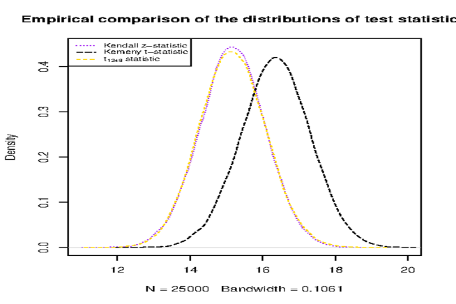
Figure 1: Demonstration that the $t_{1248}$-distribution for the Kemeny partial Wald test is in concordance with the prescribed Gauss-Markov theorem and with strictly sub-Gaussian errors consistent with a normal distribution for finite samples.

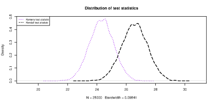
Figure 2: Visualisation of the empirical distributions with n = 2500, wherein even for large samples, we observe that the Kemeny $\tau_{\kappa}$ estimator is both more consistent and more normally distributed.

Table 1: Empirical comparison of the distribution of 25,000 test statistics for the bivariate correlations and Welch’s $t_{1248}-$test over ordinal random variables for various estimators.

Sample-size		mean	sd	median	min	max	range	skew	kurtosis
(a) n = 1250	Kemeny $t-$test	15.1668	0.8943	15.1709	11.3614	18.4783	7.1169	-0.0392	-0.0008
	Kendall $z-$test	16.3493	0.9521	16.3554	12.2476	19.8721	7.6245	-0.0436	0.0056
	Student $t_{1248}\tfrac{1}{c^{3}}$	15.1746	0.9169	15.1709	10.9595	18.9556	7.9961	0.0294	-0.0014
(b) n = 2500	Kemeny $t-$test	24.3124	0.8286	24.3218	20.6684	27.5784	6 .9101	-0.0324	-0.0012
	Kendall $z-$test	26.5708	0.8893	26.5763	22.7169	30.0486	7.3318	-0.0298	-0.0074

1.1.1 One sample non-parametric t-test

The one-sample t-test presents the estimate of a signed distance from a fixed target $\mu^{1}$ scaled by a sample dependent concentration $s_{p}$. This may be tested upon the Kemeny linear non-parametric framework via two independent means of conclusion: the first defining a permutation population vector distance, and the second reflecting individual changes upon the sample wrt individual elements $X_{i}$. Maintaining the Kemeny metric domain, constructed upon random independent samples from $\mathcal{M}_{n}^{\ast}$ defined as $\kappa(X)$, where $X$ is the arbitrary random extended real variable of length $n$, we therefore require both a (signed) distance from the expectation, and a variance, each of which are easily obtained upon the sample.

The first one-sample test statistic, scaled by the individual sample variance, is provided using equation 1a normed as in equation 3a using equation 3b. However, due to the permutation population, which is strictly sub-Gaussian, the estimator Wald statistic does not tend to a $t$-distribution, but instead a Beta-Binomial one. Once the finite support is corrected for, using $c$, the estimator is approximately normally distributed under the null hypothesis, using fixed permutation $\mu^{1}$, mapped onto a skew-symmetric matrix, for the hypothesised null value.

The second, and dual, one-sample test statistic, scaled by the individual sample variance, is constructed upon the $n\times 1$ vectors $X_{\ast},\mu_{\ast}$ produced by marginalising each $\kappa(\cdot)$ mapping over the $k=1,\ldots,n$ rows, then transposing the resulting $1\times n$ vector. This provides a linear ordering of the relative distance about the marginal expectation for the median at 0 upon the ranks. Using this topology, the Frobenius norm is employed to obtain the linear signed distance from the target mapping over all $n$ observations between permutation $m\in\mathcal{M}_{n}^{\ast}\to X_{\ast}^{n\times 1}$ and the fixed reference point $\mu_{\ast}^{1}$. As the variance is sample dependent, using the standard variance formula for the typical t-test, we obtain a test statistic with expectation 0 and a standard deviation of $1\cdot{c}$, which when scaled by the normalising continuity correction returns the null hypothesis distribution to a standard deviation to 1 and the excess kurtosis to 0, for suitably large $n$. We note that the continuity correction is largely unnecessary for suitably large $n$ upon the $\rho_{\kappa}$ based test statistic: For samples of $n\geq 100$, the continuity correction for the latter estimator’s variance is essentially equivalent to 1. However, for the Beta-Binomially distributed $\tau_{\kappa}$ test statistic, the continuity correction is substantively more limited, and should be retained according to the previously suggested thresholds.

1.1.2 Two sample non-parametric t-test

It is trivial to see that when an arbitrary $Y$ is observed to replace $\mu^{1}$, we produce a two-sample test statistic. The only mild moderation in construction is defined upon the denominator, which now reflect two independent sources of variation which must be combined. In order to resolve this identification problem, approaching the estimator from both the Kemeny permutation $n\times n$ basis and the Kemeny $n\times 1$ basis, for each random variable, we require a suitable estimator for the unknown variances. For the former $\tau_{\kappa}$ this is already provided in equation 2, simply substituting for one of the duplicated random variable $X_{j}$ the second observed mapping $\kappa(Y)$, while maintaining the closed and compact abelian nature of the Hilbert space. Inflating the expected permutation population variance for fixed $n$ by the obtained sample variance results in an affine-linear transformation of the strictly sub-Gaussian distance, which remains Beta-Binomially distributed.

In the complementary dual vector space $X_{\ast}^{n\times 1},Y_{\ast}^{n\times 1}$ upon the Frobenius norm, we now consider the test statistic for the correlation coefficient. As the marginal standard deviations are produced by the standard linear estimator, even in the presence of non-normal data, our only concern is the limiting sample size which produces a slightly larger than expected null distribution variance. To correct this error, which results from the strictly sub-Gaussian nature of the data upon $\mathcal{M}_{n}^{\ast}$, we obtain suitable expectations for the distribution by implementation of the continuity correction, noting that for $n\geq 125,$ we obtain a necessary excess variance of only 1.003395, which is determine to be negligible. This determination is confirmed by empirical evaluation of the Kolmogorov-Smironov test statistics’ difference in ECDF from the expected $t_{\nu}$-distribution, where $\nu=n-2$ exhibits non-significant differences from the null hypothesised distribution and less distance from the proposed distribution as compared to the null normal distribution which would otherwise be expected. The reason for the fairly trivial introduction of a non-parametric t-test is due to the allowance for independent sample variances which are not guaranteed equality to $n-1$, as expected upon $S_{n}$.

2 Empirical demonstrations

In this section, we provide a number of numerical demonstrations of each estimator, while establishing the validity of the constructed Wald test statistics, which follow the claimed $t_{\nu}$-distribution with better performance relative to the alternative normal distribution. It should be immediately recognised by the abelian linear model of the sample mean comparisons and the correlation coefficients that the performance is identical for either application. The main compelling difference in analysis focuses upon the invocation of the continuity correction upon both $\rho_{\kappa}$ and $\tau_{\kappa}$, and whether the strictly sub-Gaussian null hypothesis distribution is suitably continuous or not, such that $c\geq 1$.

The utility of the correction is most prevalent upon the $\tau_{\kappa}$ domain, which is theoretically justified by the basis domain being defined upon the entire collection of the $n$ elements’ inner-product between the two skew-symmetric matrices. As the population $M_{n}^{\ast}$ is atomic relative to the standard expected atomless measure for all real numbers, the finite population cardinality, largely reflected in its leptokurtotic nature, forces the distribution to maintain a stable strictly sub-Gaussian nature. However, upon $\rho_{\kappa}$ we observe the linear combination of $n$ distinct elements, which via the central limit theorem enforces faster converge to normality, at the cost of greater than theoretically appropriate variance. This ratio thus defines the expectation of the $t_{\nu}$-distribution performance, while maintaining the bijective duality as depicted in Figure 1. It should be noted that under the Glivenko-Cantelli condition, the expectation of the p-values for the appropriate distribution are 0.5 and the variance should be approximately the square root of said mean p-value.

2.1 One sample t-test and correlation coefficient

Table 2: One-sample t-test results, presenting the variance and Tchebyshev error of the test statistic distributions under $t_{n-1}$ and normality.

sample size	vars	mean	sd	median	mad	min	max	skew	kurtosis
n = 10	Variance	1.3592	0.0121	1.3584	0.0110	1.3325	1.3985	0.3155	0.7364
	$\Pr$.norm	0.0000	0.0000	0.0000	0.0000	0.0000	0.0000
	$\Pr.t_{\nu}$	0.0981	0.0909	0.0735	0.0898	0.0001	0.3532	0.8305	-0.3643
n = 15	Variance	1.1921	0.0081	1.1921	0.0071	1.1673	1.2175	-0.0278	0.6900
	$\Pr$.norm	0.0000	0.0000	0.0000	0.0000	0.0000	0.0000	4.8598	26.7915
	$\Pr.t_{\nu}$	0.2427	0.1868	0.2072	0.1823	0.0016	0.7816	0.7999	-0.1902
n = 20	Variance	1.1298	0.0078	1.1301	0.0085	1.1140	1.1499	0.3551	-0.3520
	$\Pr$.norm	0.0002	0.0003	0.0001	0.0001	0.0000	0.0024	3.6843	17.0129
	$\Pr.t_{\nu}$	0.3874	0.2643	0.3280	0.2895	0.0095	0.9621	0.4401	-0.9823
n = 25	Variance	1.0990	0.0073	1.0995	0.0063	1.0809	1.1165	-0.2661	-0.1038
	$\Pr$.norm	0.0037	0.0057	0.0015	0.0018	0.0000	0.0313	3.0361	9.9158
	$\Pr.t_{\nu}$	0.4328	0.3018	0.3699	0.3778	0.0013	0.9826	0.3236	-1.2425
n = 35	Variance	1.0656	0.0066	1.0654	0.0071	1.0479	1.0830	-0.0553	-0.0829
	$\Pr$.norm	0.0609	0.0626	0.0437	0.0404	0.0005	0.4487	2.8293	13.0304
	$\Pr.t_{\nu}$	0.4609	0.2851	0.4646	0.3650	0.0059	0.9914	0.0101	-1.2400
n = 55	Variance	1.0400	0.0066	1.0402	0.0069	1.0232	1.0550	-0.1943	-0.3074
	$\Pr$.norm	0.2429	0.1666	0.2226	0.1911	0.0034	0.7678	0.6339	-0.1038
	$\Pr.t_{\nu}$	0.4889	0.3320	0.4769	0.4496	0.0116	0.9930	0.1163	-1.4623
n = 75	Variance	1.0285	0.0063	1.0286	0.0066	1.0120	1.0421	-0.0028	-0.4108
	$\Pr$.norm	0.3932	0.2082	0.3860	0.2336	0.0405	0.8450	0.2177	-0.7730
	$\Pr.t_{\nu}$	0.5275	0.2803	0.5350	0.3693	0.0309	0.9859	-0.1254	-1.2658
n = 95	Variance	1.0210	0.0066	1.0212	0.0065	1.0071	1.0400	0.2092	-0.3071
	$\Pr$.norm	0.4269	0.2622	0.4426	0.2985	0.0038	0.9498	0.1681	-0.9971
	$\Pr.t_{\nu}$	0.4831	0.2942	0.5120	0.3818	0.0045	0.9847	0.0042	-1.2458
n = 115	Variance	1.0181	0.0060	1.0178	0.0056	1.0012	1.0348	-0.0382	0.0178
	$\Pr$.norm	0.4679	0.2651	0.4805	0.3222	0.0187	0.9875	0.0332	-1.0128
	$\Pr.t_{\nu}$	0.5072	0.2811	0.5273	0.3408	0.0242	0.9967	-0.0749	-1.1495
n = 135	Variance	1.0142	0.0070	1.0146	0.0067	0.9957	1.0311	-0.2285	0.1833
	$\Pr$.norm	0.4749	0.2836	0.5071	0.3863	0.0101	0.9896	-0.0483	-1.3526
	$\Pr.t_{\nu}$	0.5007	0.2920	0.5151	0.3475	0.0055	0.9956	-0.1069	-1.2800

A total of 55,000 permutations for 10 different sample sizes were simulated, 100 times each, from the appropriate population permutation space $\mathcal{M}_{n}^{\ast},$ denoting $X_{\ast}$ for fixed $Y_{\ast}=[1,2,\ldots,n]^{\intercal}.$ In addition to the estimated variances of the test statistics for each sample size, we also collected empirical Kolmogorov-Smironov test statistic p-values for the Gaussian and Student $t$-distributions with $\nu=n-1$ degrees of freedom. As theoretically shown, it was expected that the average p-values would favour the $t_{\nu}$ distributions, thereby showing greater empirical preference uniformly across all samples. Note that under the null hypothesis of the t-distributions, the limiting variances are defined as 1 but are typically greater than said limit. In total, the average empirical value was found to favour the Studentised signed Wald test statistic. This serves to validate our theoretical claim that the distributions constructed upon the Kemeny metric space are in fact both unbiased and $t_{\nu}$-distributed.

2.2 One sample correlation t-test with different unique variances

Table 3: $t_{\nu}$-distribution results, with $\nu=n-2$. Note that the t-distribution is almost always found to be better fitting than the corresponding normal distribution. The two sample test statistics present with average variances which are nearly identical to the one-sample test statistics as well, supporting the Glivenko-Cantelli uniformity assertion.

sample size	vars	mean	sd	median	mad	min	max	skew	kurtosis
n = 10	Variance	1.3535	0.0109	1.3534	0.0099	1.3309	1.3759	0.1027	-0.4753
	$\Pr$.norm	0.0000	0.0000	0.0000	0.0000	0.0000	0.0000	4.6246	19.5831
	$\Pr.t_{\nu}$	0.2801	0.2294	0.1958	0.2140	0.0008	0.8948	0.6806	-0.7668
n = 15	Variance	1.1911	0.0095	1.1914	0.0082	1.1695	1.2136	-0.0890	0.0313
	$\Pr$.norm	0.0000	0.0000	0.0000	0.0000	0.0000	0.0000	5.9236	36.4432
	$\Pr.t_{\nu}$	0.3668	0.3109	0.2735	0.3281	0.0014	0.9762	0.4962	-1.2212
n = 20	Variance	1.1293	0.0086	1.1294	0.0110	1.1044	1.1445	-0.3675	-0.2253
	$\Pr$.norm	0.0002	0.0008	0.0001	0.0001	0.0000	0.0073	8.3016	74.3816
	$\Pr.t_{\nu}$	0.3677	0.2533	0.3335	0.2692	0.0054	0.9865	0.4516	-0.8192
n = 25	Variance	1.0964	0.0073	1.0958	0.0068	1.0817	1.1155	0.4480	-0.0611
	$\Pr$.norm	0.0043	0.0054	0.0019	0.0024	0.0001	0.0243	1.8308	2.9469
	$\Pr.t_{\nu}$	0.4033	0.2781	0.3643	0.3178	0.0152	0.9892	0.4257	-1.0114
n = 35	Variance	1.0666	0.0072	1.0656	0.0063	1.0465	1.0795	-0.2792	0.0409
	$\Pr$.norm	0.0600	0.0547	0.0469	0.0445	0.0026	0.3133	1.8092	4.2084
	$\Pr.t_{\nu}$	0.4702	0.2826	0.4895	0.3427	0.0337	0.9766	-0.0243	-1.2251
n = 55	Variance	1.0413	0.0070	1.0421	0.0055	1.0276	1.0579	0.1384	-0.1512
	$\Pr$.norm	0.2487	0.1830	0.2071	0.1859	0.0121	0.8095	0.7698	-0.1063
	$\Pr.t_{\nu}$	0.4859	0.2943	0.4622	0.3425	0.0106	0.9963	0.1445	-1.0940
n = 75	Variance	1.0286	0.0067	1.0273	0.0043	1.0112	1.0408	-0.4327	0.2696
	$\Pr$.norm	0.3785	0.2127	0.3946	0.2782	0.0181	0.8553	0.0617	-1.1837
	$\Pr.t_{\nu}$	0.4735	0.2844	0.4688	0.3742	0.0140	0.9840	0.0840	-1.2300
n = 95	Variance	1.0208	0.0068	1.0211	0.0073	1.0000	1.0327	-0.3466	0.5340
	$\Pr$.norm	0.4343	0.2631	0.4181	0.2641	0.0011	0.9766	0.2598	-0.9052
	$\Pr.t_{\nu}$	0.5262	0.2934	0.5284	0.3734	0.0022	0.9754	-0.1241	-1.1727
n = 115	Variance	1.0185	0.0057	1.0182	0.0053	1.0054	1.0307	-0.2349	-0.2340
	$\Pr$.norm	0.4452	0.2721	0.3927	0.3266	0.0070	0.9935	0.2644	-1.2217
	$\Pr.t_{\nu}$	0.4904	0.2818	0.5004	0.3841	0.0039	0.9907	0.0501	-1.2668
n = 135	Variance	0.9880	0.1671	1.0152	0.0087	0.0000	1.0266	-5.5818	30.0358
	$\Pr$.norm	0.4976	0.2868	0.5307	0.3380	0.0036	0.9965	-0.0629	-1.2200
	$\Pr.t_{\nu}$	0.5296	0.2901	0.5493	0.3842	0.0056	0.9982	-0.2029	-1.1905

A similar simulation was conducted for the two-sample t-test, randomly selecting two arbitrary permutations with ties for each specified $n$ and computing the $t_{n-2}$-distribution of test statistics. Significance of differences from the normal distribution and appropriate t-distribution were reported, and the summary of the distribution of deviations from the theoretical expectations are provided. We observe that the variances between the one and two sample tests are nearly identical for every sample size, and that as the degrees of freedom increase, the t-distributions appear to regularly converge to normality: this is observed by the variance of the distributions tending to 1.

In comparing the distributions of the sinusoidally transformed Kemeny $\tau_{\kappa}$ correlation to the corresponding $t$-distribution, we observe that the strictly sub-Gaussian nature of the estimator is maintained, thereby presenting as leptokurtotic, with increased concentration. Thus, while the direct $t$-statistics do not require a continuity correction, the transformations of the $z$-distribution with freely estimated variances do in fact require a continuity correction, to maintain the expected normality distribution under the null hypothesis. Thus, the sinusoidal transform is directly observed to link the two orthonormal topological estimators as a distinct duality, although the discrete to continuous representations of the respective Kemeny and Frobenius norms are imperfect for finite samples.

2.2.1 Sleep data demonstration

The Sleep data set, available in R base, provides an ideal representation of the correlation coefficient between two-groups over 20 individuals. Thus, the distance is 141 by the Kemeny metric, with marginal standard deviations of 8.357159 for sleep and 7.254763 for group drug exposure. The non-parametric $\rho_{\kappa}=0.4253639,t_{18}=1.9941,p=0.06152.$ Using the original scores, the Pearson product-moment correlation obtains $r=0.4016626,t_{18}=1.8608,p=0.07919.$ This confirms the loss of power upon the Frobenius norm applied to non-normal data, as measured by the sample difference in sleep observed after treated with one of two optical isomer conditions. Given the provided marginal summary statistics, the Kemeny

$$\tau_{\kappa}=.2578947,z=\tfrac{141}{\sqrt{\tfrac{938.6}{0.2578947}}}\cdot(\tfrac{7}{11})^{.5}=1.864459,p=0.06225727,$$

again supporting the conclusion that the non-normality of the data enables more powerful monotonic linearity detection upon the Kemeny metric, especially in the presence of ties for discrete comparisons. The relationship between the individual and population permutations depicts a mild differences, indicating a potential outlier in the relative non-linear change in the Frobenius rank domain compared to the lower estimated population permutation domain, or simply the duality gap present in finite samples: $\sin(.2578947\cdot\tfrac{\pi}{2})=0.3941107<0.4253639.$

Table 4: 15,500 bootstrap replications of the point-biserial correlation upon [4] Sleep data

vars	mean	sd	median	trimmed	mad	min	max	range	skew	kurtosis
$\tau_{\kappa}$	0.245	0.116	0.253	0.250	0.117	-0.321	0.526	0.847	-0.466	0.184
$\rho_{\kappa}$	0.417	0.196	0.435	0.427	0.194	-0.543	0.875	1.419	-0.503	0.237
Pearson’s $r$	0.393	0.187	0.409	0.402	0.185	-0.599	0.898	1.497	-0.499	0.356
Spearman’s $\rho$	0.417	0.196	0.435	0.427	0.194	-0.543	0.875	1.419	-0.503	0.237
Kendall $\tau_{b}$	0.358	0.168	0.373	0.366	0.166	-0.470	0.764	1.234	-0.502	0.252

As expected, under replication the Kemeny $\tau_{\kappa}$ coefficient was the most normally distributed, and both metric spaces upon the Kemeny basis were exhibited greater population stability in both variance and range of estimated realisations. The 95% quantiles for the bootstrapped coefficients confirmed the previous population expectations under the Wald tests as well. For the Kemeny $\tau_{\kappa}$, 95%CI = (-0.005,0.442), and for Kemeny $\rho_{\kappa}$, 95%CI = (-0.010,0.749), the confidence intervals parallel the close, but non-significant, rejection of the null hypothesis of a correlation coefficient of 0.

3 Discussion

We have presented formulations for addressing correlation coefficients under the bilinearity conditions of the permutation space and the individual sample elements, in traditional non-parametric scenarios. This allows for the construction of $t_{\nu}$-distribution test statistics for the correlations, which are compact and totally bounded unbiased minimum variance estimators which do not require Gaussian data. Test performance is ideal, and the allowance for ties under a Hilbert space representation allows for the probability mapping to uniquely represent the uniformly most powerful correlation test.

References

- [1] Persi Diaconis “Group Representations in Probability and Statistics” Institute of Mathematical Statistics, Hayward, CA, 1988
- [2] John G Kemeny “Generalized random variables” In Pacific Journal of Mathematics 9.4 Mathematical Sciences Publishers, 1959, pp. 1179–1189 DOI: 10.2140/pjm.1959.9.1179
- [3] J.. Ord “The Discrete Student’s t Distribution” In The Annals of Mathematical Statistics 39.5 Institute of Mathematical Statistics, 1968, pp. 1513–1516 DOI: 10.1214/aoms/1177698133
- [4] Student “The Probable Error of a Mean” In Biometrika 6.1 JSTOR, 1908, pp. 1 DOI: 10.2307/2331554
- [5] Larry Wasserman “All of Statistics” Springer New York, 2004 DOI: 10.1007/978-0-387-21736-9