Adaptively Weighted Audits of Instant-Runoff Voting Elections: AWAIRE

Abstract

An election audit is risk-limiting if the audit limits (to a pre-specified threshold) the chance that an erroneous electoral outcome will be certified. Extant methods for auditing instant-runoff voting (IRV) elections are either not risk-limiting or require cast vote records (CVRs), the voting system’s electronic record of the votes on each ballot. CVRs are not always available, for instance, in jurisdictions that tabulate IRV contests manually.

We develop an RLA method (AWAIRE) that uses adaptively weighted averages of test supermartingales to efficiently audit IRV elections when CVRs are not available. The adaptive weighting ‘learns’ an efficient set of hypotheses to test to confirm the election outcome. When accurate CVRs are available, AWAIRE can use them to increase the efficiency to match the performance of existing methods that require CVRs.

We provide an open-source prototype implementation that can handle elections with up to six candidates. Simulations using data from real elections show that AWAIRE is likely to be efficient in practice. We discuss how to extend the computational approach to handle elections with more candidates.

Adaptively weighted averages of test supermartingales are a general tool, useful beyond election audits to test collections of hypotheses sequentially while rigorously controlling the familywise error rate.

1 Introduction

Ranked-choice or preferential elections allow voters to express their relative preferences for some or all of the candidates, rather than simply voting for one or more candidates. Instant-runoff voting (IRV) is a common form of ranked-choice voting. IRV is used in political elections in several countries, including all lower house elections in Australia.

A risk-limiting audit (RLA) is any procedure with a guaranteed minimum probability of correcting the reported outcome if the reported outcome is wrong. RLAs never alter correct outcomes. (Outcome means the political outcome—who won—not the particular vote tallies.) The risk limit $\alpha$ is the maximum chance that a wrong outcome will not be corrected. Risk-limiting audits are legally mandated or authorised in approximately 15 U.S. states and have been used internationally. RAIRE [2] is the first method for conducting RLAs for IRV contests. RAIRE generates ‘assertions’ which, if true, imply that the reported winner really won. Such assertions are the basis of the SHANGRLA framework for RLAs [5].

A cast vote record (CVR) is the voting system’s interpretation of the votes on a ballot. RAIRE uses CVRs to select the assertions to test. Voting systems that tabulate votes electronically (e.g., using optical scanners) typically generate CVRs, but in some jurisdictions (e.g., most lower house elections in Australia) votes are tabulated manually, with no electronic vote records. Because RAIRE requires CVRs, it cannot be used to check manually tabulated elections. Moreover, while RAIRE generates a set of assertions that are expected to be easy to check statistically if the CVRs are correct, if the CVRs have a high error rate, then the assertions it generates may not hold even if the reported winner actually won, leading to an unnecessary full hand count.

In this paper we develop an approach to auditing IRV elections that does not require CVRs. Instead, it adapts to the observed voter preferences as the audit sample evolves, identifying a set of hypotheses that are efficient to test statistically. The approach has some statistical novelty and logical complexity. To help the reader track the gist of the approach, here is an overview:

• Tabulating an IRV election results in a candidate elimination order. A candidate elimination order that yields a winner other than the reported winner is an alt-order. If there is sufficiently strong evidence that no alt-order is correct, we may safely conclude that the reported winner really won.

• Each alt-order can be characterised by a set of requirements, necessary conditions for that elimination order to be correct. If the data refute at least one requirement for each alt-order, the reported outcome is confirmed.

• We construct a test supermartingale for each requirement; a (predictable) convex combination of the test supermartingales for the requirements in an alt-order is a test supermartingale for that alt-order.

• As the audit progresses, we update the convex combination for each alt-order to give more weight to the test supermartingales that are giving the strongest evidence that their corresponding requirements are false.

• The audit has attained the risk limit $\alpha$ when the intersection test supermartingale for every alt-order exceeds $1/\alpha$ (or when every ballot has been inspected and the correct outcome is known).

The general strategy of adaptively re-weighting convex combinations of test supermartingales gives powerful tests that rigorously control the sequential familywise error rate. It is applicable to a broad range of nonparametric and parametric hypothesis testing problems. We believe this is the first time these ideas have been used in a real application.

To our knowledge, the SHANGRLA framework has until now been used to audit only social choice functions for which correctness of the outcome is implied by conjunctions of assertions: if all the assertions are true, the contest result is correct. The approach presented here—controlling the familywise error rate within groups of hypotheses and the per-comparison error rate across such groups—allows SHANGRLA to be used to audit social choice functions for which correctness is implied by disjunctions of assertions as well as conjunctions. This fundamentally extends SHANGRLA.

2 Auditing IRV contests

We focus on IRV contests. The set of candidates is $\mathcal{C}$, with total number of candidates $C:=|\mathcal{C}|$. A ballot $b$ is an ordering of a subset of candidates. The number of ballots cast in the election is $B$.

Each ballot initially counts as a vote for the first-choice candidate on that ballot. The candidate with the fewest first-choice votes is eliminated (the others remain ‘standing’). The ballots that ranked that candidate first are now counted as if the eliminated candidate did not appear on the ballot: the second choice becomes the first, etc. This ‘eliminate the candidate with the fewest votes and redistribute’ continues until only one candidate remains standing, the winner. (If at any point there are no further choices of candidate specified on a ballot, then the ballot is exhausted and no longer contributes any votes.) Tabulating the votes results in an elimination order: the order in which candidates are eliminated, with the last candidate in the order being the winner.

2.1 Alternative elimination orders

In order to audit an IRV election we need to show that if any candidate other than the reported winner actually won, the audit data would be ‘surprising,’ in the sense that we can reject (at significance level $\alpha$) the null hypothesis that any other candidate won.

Example 1

Consider a four-candidate election, with candidates $1$, $2$, $3$, $4$, where $1$ is the reported winner. We must be able to reject every elimination order in which any candidate other than $1$ is eliminated last (every alt-order): $[1,2,3,4]$, $[1,2,4,3]$, $[1,3,2,4]$, $[1,3,4,2]$, $[1,4,2,3]$, $[1,4,2,3]$, $[2,1,3,4]$, $[2,1,4,3]$, $[2,3,1,4]$, $[2,4,1,3]$, $[3,1,2,4]$, $[3,1,4,2]$, $[3,2,1,4]$, $[3,4,1,2]$, $[4,1,2,3]$, $[4,1,3,2]$, $[4,2,1,3]$, $[4,3,1,2]$. The other 6 elimination orders lead to $1$ winning: they are not alt-orders. ∎

To assess an alt-order, we construct requirements that necessarily hold if that alt-order is correct—then test whether those requirements hold. If one or more requirements for a given alt-order can be rejected statistically, then that is evidence that the alt-order is not the correct elimination order. Blom et al. [2] show that elimination orders can be analysed using two kinds of statements, of which we use but one:

‘Directly Beats’: $\textbf{DB}(i,j,\mathcal{S})$ holds if candidate $i$ has more votes than candidate $j$, assuming that only the candidates $\mathcal{S}\supseteq\{i,j\}$ remain standing. It implies that $i$ cannot be the next eliminated candidate (since $j$ would be eliminated before $i$) if only the candidates $\mathcal{S}$ remain standing.

2.2 Sequential testing using test supermartingales

Each requirement can be expressed as the hypothesis that the mean of a finite list of bounded numbers is less than $1/2$. Each such list results from applying an assorter (see Stark [5]) to the preferences on each ballot. The assorters we use below all take values in $[0,1]$. For example, consider the requirement $\textbf{DB}(1,2,\mathcal{C})$ that candidate $1$ beats candidate $2$ on first preferences. That corresponds to assigning a ballot the value $1$ if it shows a first preference for candidate $2$, the value $0$ if it shows a first preference for $1$, and the value $1/2$ otherwise. If the mean of the resulting list of $B$ numbers is less than $1/2$, then the requirement $\textbf{DB}(1,2,\mathcal{C})$ holds.

A stochastic process $(M_{t})_{t\in\mathbb{N}}$ is a supermartingale with respect to another stochastic process $(X_{t})_{t\in\mathbb{N}}$ if $\operatorname{\mathbb{E}}(M_{t}\mid X_{1},\dots,X_{t-1})\leqslant M_{t-1}$. A test supermartingale for a hypothesis is a stochastic process that, if the null hypothesis is true, is a nonnegative supermartingale with $M_{0}:=1$. By Ville’s inequality [7], which generalises Markov’s inequality to nonnegative supermartingales, the chance that a test supermartingale ever exceeds $1/\alpha$ is at most $\alpha$ if the null hypothesis is true. Hence, we reject the null hypothesis if at some point $t$ we observe $M_{t}\geqslant 1/\alpha$. The maximum chance of the rejection being in error is $\alpha$.

Let $X_{1},X_{2},\dots$ be the result of applying the assorter for a particular requirement to the votes on ballots drawn sequentially at random without replacement from all of the $B$ cast ballots. We test the requirement using the ALPHA test supermartingale for the hypothesis that the mean of the $B$ values of the assorter is at most $\mu_{0}$ is

$$M_{j}=\prod_{i=1}^{j}\left(\frac{X_{i}}{\mu_{i}}\cdot\frac{\eta_{i}-\mu_{i}}{1-\mu_{i}}+\frac{1-\eta_{i}}{1-\mu_{i}}\right),\quad j=1,2,\dots,B,$$

where

$$\mu_{j}=\frac{B\mu_{0}-\sum_{i=1}^{j-1}X_{i}}{B-j+1}$$

is the mean of the population just before the $j$th ballot is drawn (and is thus the value of $\operatorname{\mathbb{E}}X_{j}$) if the null hypothesis is true. The value of $M_{j}$ decreases monotonically in $\mu_{0}$, so it suffices to consider the largest value of $\mu_{0}$ in the null hypothesis, i.e., $\mu_{0}=1/2$ [6]. The value $\eta_{j}$ can be thought of as a (possibly biased) estimate of the true assorter mean for the ballots remaining in the population just before the $j$th ballot is drawn. We use the ‘truncated shrinkage’ estimator suggested by Stark [6]:

$$\eta_{j}=\min\left[\max\left(\frac{d\eta_{0}+\sum_{i=1}^{j-1}X_{i}}{d+j-1},\,\mu_{j}+\epsilon_{j}\right),\,1\right].$$

The parameters $\epsilon_{j}=(\eta_{0}-\mu)/(2\sqrt{d+j-1})$ form a nonnegative decreasing sequence with $\mu_{j}<\eta_{j}\leqslant 1$. The parameters $\eta_{0}$ and $d$ are tuning parameters. The ALPHA supermartingales span the family of betting supermartingales, discussed by [9]: setting $\eta_{j}$ in ALPHA is equivalent to setting $\lambda_{j}$ in betting supermartingales [6].

3 Auditing via adaptive weighting (AWAIRE)

3.1 Eliminating elimination orders using ‘requirements’

We can formulate auditing an IRV contest as a collection of hypothesis tests. To show that the reported winner really won, we consider every elimination order that would produce a different winner (every alt-order). The audit stops without a full hand count if it provides sufficiently strong evidence that no alt-order occurred. Suppose there are $m$ alt-orders. Let $H_{0}^{i}$ denote the hypothesis that alt-order $i$ is the true elimination order, $i=1,\dots,m$. These partition the global null hypothesis,

$$H_{0}=H_{0}^{1}\cup\dots\cup H_{0}^{m}.$$

If we reject all the null hypotheses $H_{0}^{1},\dots,H_{0}^{m}$, then we have also rejected $H_{0}$ and can certify the outcome of the election.

For each alt-order $i$, we have a set of requirements $R_{i}=\{R_{i}^{1},R_{i}^{2},\dots,R_{i}^{r_{i}}\}$ that necessarily hold if $i$ is the true elimination order, i.e.,

$$H_{0}^{i}\subseteq R_{i}^{1}\cap R_{i}^{2}\cap\dots\cap R_{i}^{r_{i}}.$$

If any of these requirements is false, then alt-order $i$ is not the true elimination order. If

$$H_{0}^{i}=R_{i}^{1}\cap R_{i}^{2}\cap\dots\cap R_{i}^{r_{i}}$$

then $R_{i}$ is a complete set of requirements: they are necessary and sufficient for elimination order $i$ to be correct. One way to create a complete set is to take all DB requirements that completely determine each elimination in the given elimination order.

Example 2

A complete set of requirements for the elimination order $[1,2,3,4]$ is: $\textbf{DB}(4,3,\{3,4\})$, $\textbf{DB}(4,2,\{2,3,4\})$, $\textbf{DB}(3,2,\{2,3,4\})$, $\textbf{DB}(4,1,\{1,2,3,4\})$, $\textbf{DB}(3,1,\{1,2,3,4\})$, and $\textbf{DB}(2,1,\{1,2,3,4\})$. If we reject any of these, then we can reject the elimination order $[1,2,3,4]$. ∎

We can rule out alt-order $i$ by rejecting the intersection hypothesis $R_{i}^{1}\cap\dots\cap R_{i}^{r_{i}}$. The test supermartingales for the individual requirements are dependent because all are based on the same random sample of ballots. Section 3.2 shows how to test the intersection hypothesis, taking into account the dependence.

3.1.1 ‘Requirements’ vs ‘assertions’.

SHANGRLA [5] uses the term ‘assertions.’ Requirements and assertions are statistical hypotheses about means of assorters applied to the votes on all the ballots cast in the election. ‘Assertions’ are hypotheses whose conjunction is sufficient to show that the reported winner really won: if all the assertions are true, the reported winner really won. ‘Requirements’ are hypotheses that are necessary if the reported winner really lost—in a particular way, e.g., because a particular alt-order occurred. Loosely speaking, assertions are statements that, if true, allow the audit to stop; while requirements are statements that, if false, allow the audit to stop. To stop without a full hand count, an assertion-based audit needs to show that every assertion is true. In contrast, a requirement-based audit needs to show that at least one requirement is false in each element $H_{0}^{i}$ of a partition of the null hypothesis $H_{0}=\cup_{i}H_{0}^{i}$. (In AWAIRE, the partition corresponds to the alt-orders.)

3.2 Adaptively weighted test supermartingales

Given the sequentially observed ballots, we can construct a test supermartingale (such as ALPHA) for any particular requirement. To test a given hypothesis $H_{0}^{i}$, we need to test the intersection of the requirements in the set $R_{i}$. We now describe how we test that intersection hypothesis, despite the dependence among the test supermartingales for the separate requirements. The test involves forming weighted combinations of the terms in the test supermartingales for individual requirements in such a way that the resulting process is itself a test supermartingale for the intersection hypothesis. This is somewhat similar to the methods of combining test supermartingales described by Vovk & Wang [8].

The quantities defined in this section, such as $E_{r,t}$, are for a given set of requirements $R_{i}$ and thus implicitly depend on $i$. For brevity, we omit $i$ in the notation.

At each time $t$, a ballot is drawn without replacement, and the assorter corresponding to each $R_{i}^{r}$, $r=1,\dots,r_{i}$ is computed, producing the values $X_{t}^{r}$, $r=1,\dots,r_{i}$. Let $(E_{r,t})$ be the test supermartingale for requirement $r$. The test supermartingale can be written as a telescoping product:

$$E_{r,t}:=\prod_{k=0}^{t}e_{r,k},$$

with $E_{r,0}:=1$ for all $r$ and

$$\mathbb{E}(e_{r,k}\mid(X_{\ell}^{r})_{\ell=0}^{k-1})\leqslant 1,$$ (1)

where the conditional expectation is computed under the hypothesis that requirement $r$ is true. (This last condition amounts to the supermartingale property.) We refer to these as base test supermartingales.

For each $k$, let $\{w_{r,k}\}_{r=1}^{r_{i}}$ be nonnegative predictable numbers: $w_{r,t}$ can depend on the values $\{X_{k}^{r}\}$, $r=1,\dots,r_{i}$, $k=0,\dots,t-1$ but not on data collected on or after time $t$. Define the stochastic process formed by multiplying convex combinations of terms from the base test supermartingales using those weights:

$$E_{t}:=\prod_{k=1}^{t}\frac{\sum_{r=1}^{r_{i}}w_{r,k}e_{r,k}}{\sum_{r=1}^{r_{i}}w_{r,k}},\quad t=0,1,\dots,$$

with $E_{0}:=1$. This process, which we call an intersection test supermartingale, is a test supermartingale for the intersection of the $r_{i}$ hypotheses: Clearly $E_{t}\geqslant 0$ and $E_{0}:=1$, and if all the hypotheses are true,

$$\operatorname{\mathbb{E}}\left(E_{t}\mid(X_{k}^{r})_{k=1}^{t-1},r=1,\dots,r_{i}\right) = \operatorname{\mathbb{E}}\left(E_{t-1}\frac{\sum_{r=1}^{r_{i}}w_{r,k}e_{r,k}}{\sum_{r=1}^{r_{i}}w_{r,k}}\mid(X_{k}^{r})_{k=1}^{t-1},r=1,\dots,r_{i}\right)$$

$$= E_{t-1}\operatorname{\mathbb{E}}\left(\frac{\sum_{r=1}^{r_{i}}w_{r,k}e_{r,k}}{\sum_{r=1}^{r_{i}}w_{r,k}}\mid(X_{k}^{r})_{k=1}^{t-1},r=1,\dots,r_{i}\right)$$

$$= E_{t-1}\frac{\sum_{r=1}^{r_{i}}w_{r,k}\;\operatorname{\mathbb{E}}\left(e_{r,k}\mid(X_{k}^{r})_{k=1}^{t-1}\right)}{\sum_{r=1}^{r_{i}}w_{r,k}}$$

$$\leqslant E_{t-1}\frac{\sum_{r=1}^{r_{i}}w_{r,k}}{\sum_{r=1}^{r_{i}}w_{r,k}}=E_{t-1},$$

where the penultimate step follows from Equation 1. Thus $(E_{t})$ is a test supermartingale for the intersection of the requirements. The base test supermartingale for any requirement that is false is expected to grow in the long run (the growth rate depends on the true assorter values and the choice of base test supermartingales). We aim to make $E_{t}$ grow as quickly as the fastest-growing base supermartingale by giving more weight to the terms from the base supermartingales that are growing fastest.

For example, we could take the weights to be proportional to the base values in the previous timestep, $w_{r,t}=E_{r,t-1}$. More generally, we can explore other functions of those previous values, see below for some options. Unless stated otherwise, we set the initial weights for the requirement to be equal.

This describes how we test an individual alt-order. The same procedure is used in parallel for every alt-order. Because the audit stops without a full handcount only if every alt-order is ruled out, there is no multiplicity issue.

3.2.1 Setting the weights.

We explored three ways of picking the weights:

Linear.

Proportional to previous value, $w_{r,t}:=E_{r,t-1}$.

Quadratic.

Proportional to the square of the previous value, $w_{r,t}:=E_{r,t-1}^{2}$.

Largest.

Take only the largest base supermartingale(s) and ignore the rest, $w_{r,t}:=1$ if $r\in\operatorname*{arg\,max}_{r^{\prime}}E_{r^{\prime},t-1}$; otherwise, $w_{r,t}:=0$.

3.2.2 Using ALPHA with AWAIRE.

The adaptive weighting scheme described above can work with any test supermartingales. In our implementation, we use ALPHA with the truncated shrinkage estimator to select $\eta_{t}$ (see Section 2.2); it would be interesting to study the performance of other test supermartingales, for instance, some that use the betting strategies in Waudby-Smith & Ramdas [9].

In our experiments (see Section 4), the intersection test supermartingales were evaluated after observing each ballot. However, for practical reasons, we updated the weights only after observing every 25 ballots rather than every ballot; this does not affect the validity (the risk limit is maintained), only the adaptivity. Initial experiments seem to indicate that updating the weights more frequently often slightly favours lower sample sizes, but not always.

3.2.3 Using CVRs.

If accurate CVRs are available, then we can use them to ‘tune’ AWAIRE and ALPHA to be more efficient for auditing the given contest. We explore several options in Section 4.3. If CVRs are available and are ‘linked’ to the paper ballots in such a way that the CVR for each ballot card can be identified, AWAIRE can also be used with a ballot-level comparison audit, which could substantially reduce sample sizes compared to ballot-polling. See, e.g., Stark [5]. We have not yet studied the performance of AWAIRE for ballot-level comparison audits, only ballot-polling audits.

4 Analyses and results

To explore the performance of AWAIRE, we simulated ballot-polling audits using a combination of real and synthetic data (see below). Each sampling experiment was repeated for 1,000 random permutations of the ballots, each corresponding to a sampling order (without replacement). For each contest, the same 1,000 permutations were used for every combination of tests and tuneable parameters.

In each experiment, sampling continued until either the method confirmed the outcome or every ballot had been inspected. We report the mean sample size (across the 1,000 permutations) for each method.

The ballots were selected one at a time without replacement, and the base test supermartingales were updated accordingly. However, to allow the experiments to complete in a reasonable time, we only updated the weights after every 25 ballots were sampled. This is likely to slightly inflate the required sample sizes due to the reduced adaptation.

We repeated all of our analyses with a risk limit of 0.01, 0.05, 0.1, and 0.25. The results were qualitatively similar across all choices, therefore we only show the results for $\alpha=0.01$.

4.1 Data and software

We used data from the New South Wales (NSW) 2015 Legislative Assembly election in Australia. We took only the 71 contests with 6 or fewer candidates (due to computational constraints: future software will support elections with more candidates). The contests each included about 40k–50k ballots. Our software implementation of AWAIRE is publicly available.

We supplemented these data with 3 synthetic ‘pathological’ contests that were designed to be difficult to audit, using the same scheme as Everest et al. [4]. Each contest had 6 candidates and 56k ballots, constructed as follows. Candidates: $a$ the (true) winner, $b$ an alternate winner, and candidates $c_{1},c_{2},c_{3},c_{4}$. Ballots:

• $16000+2m$ ballots of the form $[a]$,

• $8000-2m$ ballots of the form $[b]$,

• 8000 ballots of the form $[c_{i},b,a]$ for each $i\in\{1,2,3,4\}$.

We used $m\in\{2.5,25,250\}$ to define the 3 pathological contests.

In each of these contests, $b$ is eliminated first, then each of the $c_{i}$ is eliminated, making $a$ the winner. If any $c_{i}$ is eliminated first by mistake (e.g., due to small errors in the count), then $b$ does not get eliminated and instead will collect all of the votes after each elimination and become the winner. A random sample of ballots, such as is used in an audit, will likely often imply the wrong winner.

We calculated the margin of each contest using margin-irv [3] to allow for easier interpretation of the results. The margin is the minimum number of ballots that need to be changed so that the reported winner is no longer the winner, given they were the true winner originally. For easier comparison across contests, we report the margin as proportion of the total ballots rather than as a count.

4.2 Comparison of weighting schemes

We tested AWAIRE with the three weighting schemes described earlier (Linear, Quadratic, and Largest). For the test supermartingales, we used ALPHA with $\eta_{0}=0.52$ and $d=50$. For each simulation, we first set the true winner to be the reported winner, and then repeated it with the closest runner-up candidate (based on the margin) as the reported winner. This allowed us to explore scenarios where the reported winner was false, in order to verify the risk limit (in all cases, the proportion of such simulations the led to certifying the wrong winner was lower than the risk limit).

Figure 1 illustrates an example of how the test supermartingales evolved in two simulations. Panel (a) is a more typical scenario, while panel (b) is an illustration of the rare scenarios where Largest is worst (due to competing and ‘wiggly’ base supermartingales).

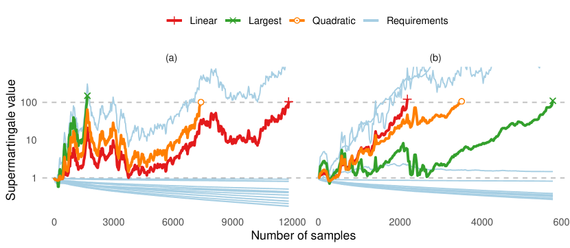
Figure 1: Examples of test supermartingales for a set of requirements. The plots show how our test supermartingales evolved as we sampled increasingly more ballots in a particular audit with risk limit $\alpha=0.01$. Each panel refers to a particular null hypothesis (i.e., a single alt-order) for a particular contest. The lines in light blue show the test supermartingales for each requirement used to test that hypothesis; the bold lines show our adaptively weighted combination across all requirements (using the weighting schemes as indicated by colour). Panel (a): NSW 2015 Upper Hunter contest (true elimination order $[1,2,3,0,4,5]$) with a hypothesised order $[1,2,3,0,5,4]$. Panel (b): NSW 2015 Prospect contest (true elimination order $[3,0,4,1,2]$) with a hypothesised order $[0,3,4,2,1]$. The horizontal lines indicate the start (1) and target ($1/\alpha=100$) values; we stop sampling and reject the null hypothesis when the intersection test supermartingale exceeds the target value.

Figure 2 summarises the performance of the different weighting schemes across a large set of contests. Some more details for a selected subset of contests are shown in top part of Table 1.

The three weighting schemes differ in how ‘aggressively’ they favour the best-looking requirements at each time point. In our experiments, the more aggressive schemes consistently performed better, with the Largest scheme achieving the best (lowest) mean sample sizes. On this basis, and the simplicity of the Largest scheme, we only used this scheme for the later analyses.

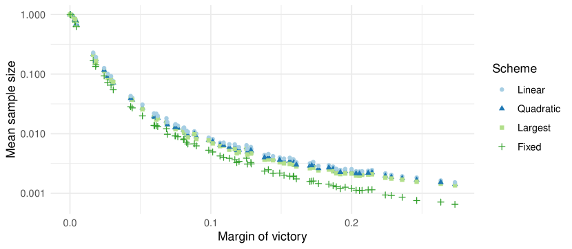
Figure 2: Comparison of weighting schemes. The mean sample size (across 1,000 simulations; shown on a log scale) versus the margin, both shown as a proportion out of the total ballots in a contest. Each point depicts a single contest and weighting scheme, the latter distinguished by colour and point type as indicated. The ‘Fixed’ scheme is only shown for reference: adaptive weighting was disabled and only the best requirements were used.

A key feature of AWAIRE is that it uses the observed ballots to ‘learn’ which requirements are the easiest to reject for each elimination order and adapts the weights throughout the audit to take advantage. To assess the statistical ‘cost’ of the learning, we also ran simulations that used a fixed weight of 1 for the test supermartingales for the requirements that proved easiest to reject, and gave zero weight to the other requirements (we call this the ‘Fixed’ scheme). The performance in this mode is shown in Figure 2 as green crosses. The Fixed version gave smaller mean sample sizes, getting as small as 55% of the Largest. This shows that adaptation less than doubles the sample size.

Table 1: Selected results. The mean sample size from experiments using a risk limit of $\alpha=0.01$, across a subset of contests, in 1,000 replications. The contest margins range from very close (Lismore) to a very wide margin (Castle Hill). The top part of the table shows results from analyses that did not use CVRs; the bottom part shows results from analyses using CVRs without errors. The column labeled $d$ is the value of the ALPHA $d$ parameter.

Contest:			Lismore	Monaro	Auburn	Maroubra	Cessnock	Castle Hill
No. candidates:			6	5	6	5	5	5
Margin:			0.44%	2.43%	5.15%	10.1%	20.0%	27.3%
Total ballots:			47,208	46,236	44,011	46,533	45,942	48,138
Method	Weights	$d$	Mean sample size
No CVRs
AWAIRE	Linear	50	34,246	5,822	1,354	378	117	73
	Quadratic	50	32,988	5,405	1,195	343	107	69
	Largest	50	32,534	5,217	1,130	320	98	65
With error-free CVRs
AWAIRE	Largest	50	32,312	5,172	1,074	283	60	33
	Largest	500	31,790	4,458	942	265	59	33
	Fixed	50	29,969	4,317	876	230	55	31
	Fixed	500	29,756	3,912	781	212	54	31
RAIRE	—	50	31,371	4,260	876	230	56	34
	—	500	31,034	3,862	781	212	54	33

4.3 Using CVRs (without errors)

We compare AWAIRE to RAIRE [2], the only other extant RLA method for IRV contests. Since RAIRE requires CVRs, we considered several ways in which we could use AWAIRE when CVRs are available. We explored choices for the following:

Starting weights.

Using the CVRs we can calculate the (reported) margin for each requirement, allowing us to determine the easiest requirement to reject for each null hypothesis (assuming the CVRs are accurate). We gave each such requirement a starting weight of 1, and the other requirements a starting weight of 0. Other choices are possible (e.g., weights set according to some function of the margins) but we did not explore them.

Weighting scheme.

If the CVRs are accurate, then it would be optimal to keep the starting weights fixed across time (similar to RAIRE). Alternatively, we can allow the weights to adapt as usual to the observed ballots, in case the CVRs are inaccurate. We explored both choices, using only the Largest weighting scheme (which performed best in our comparison, above).

Test supermartingales.

Having CVRs available allows us to tune ALPHA for each requirement by setting $\eta_{0}$ to the reported assorter mean (based on the CVRs). We allowed ALPHA to adapt by setting $d=500$ (adapt slowly) or $d=50$ (adapt quickly). For any requirements that the CVRs claim are true (i.e., consistent with the null hypothesis, with the assorter mean at most 0.5), we used a default value of $\eta_{0}=0.52$.

For comparison, we ran RAIRE with the same set of choices for the test supermartingales. For this analysis, we used accurate CVRs (no errors), the best-case scenario for RAIRE and for any choices where adaptation is slow or ‘switched off’ (such as keeping the weights fixed).

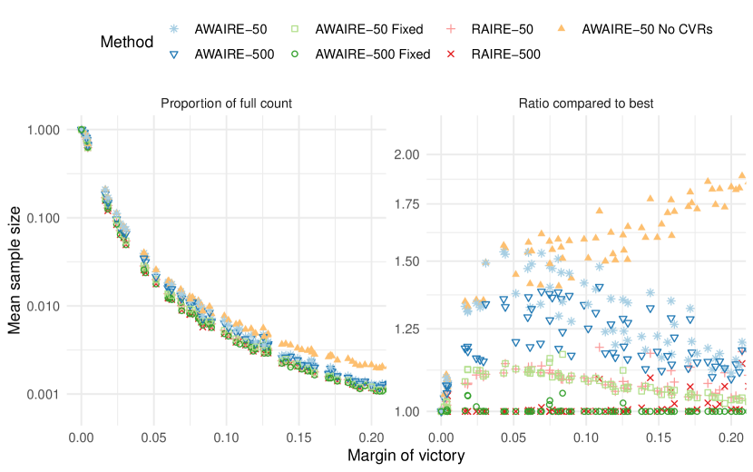
Figure 3: Comparison of methods when using accurate CVRs. Left panel: similar to Figure 2 but now showing different variants of AWAIRE all using the Largest scheme, and RAIRE. Right panel: showing mean sample size as a ratio compared to the best method for each contest. ‘Fixed’ means the weights were kept fixed throughout the audit. ‘No CVRs’ means AWAIRE was not provided the CVRs to set the starting weights. The numbers 50/500 specify the value $d$ used for ALPHA.

Figure 3 summarises the results, with a selected subset shown in the bottom part of Table 1. RAIRE and AWAIRE Fixed are on par when the CVRs are perfectly accurate, with both methods being equal most of the time. For margins up to $10\%$, RAIRE is ahead (albeit slightly) more often than AWAIRE Fixed is; for margins above $10\%$, AWAIRE Fixed is instead more often slightly ahead.

For both AWAIRE and RAIRE, the ‘less adaptive’ versions performed better than their ‘more adaptive’ versions (there is no need to adapt if there are no errors). The largest ratio between the best setup and ‘AWAIRE-50 No CVRs’ is 2.14, which occurs around a margin of 27.3%. However, at that margin, it translates to a difference of less than 35 ballots.

Interestingly, the difference between the various versions of AWAIRE is small. Across the different margins, they maintain the relative order from the least informed (No CVRs) to the most informed and least adaptive (Fixed weights, $d=500$). The cost of non-information in terms of mean sample size is surprising low, particularly when the margin of victory is small: there is little difference between ‘AWAIRE-50 No CVRs’ and ‘AWAIRE-50’. As the margin grows, the relative difference becomes more substantial but the ratio never exceeds 1.97, and at this stage the absolute difference is small (within 50 ballots).

Table 1 gives more detail on a set of elections. For the smallest margin election, AWAIRE Fixed using CVRs outperforms RAIRE, which outperforms AWAIRE Largest using CVRs, which outperforms AWAIRE without CVRs; but the relative difference in the number of ballots required to verify the result is small (about 14%). In this case, the variants of AWAIRE have similar workloads, with or without CVRs. For larger margins ($>$ 5%), the auditing effort falls, and the relative differences between AWAIRE and RAIRE become negligible.

Overall, while AWAIRE with no CVRs can require much more auditing effort than when perfect CVRs are available, for small margins the relative cost difference is small, and for larger margins the absolute cost difference is small. This shows that AWAIRE is certainly a practical approach to auditing IRV elections without the need for CVRs (if doing a ballot-polling audit).

4.4 Using CVRs with permuted candidate labels

We sought to repeat the previous comparison but with errors introduced into the CVRs. There are many possible types of errors and, as far as we are aware, no existing large dataset from which we could construct a realistic error model. A thorough analysis of possible error models is beyond the scope of this paper. For illustrative purposes, we explored scenarios where the candidate labels are permuted in the CVRs, the same strategy adopted by Everest et al. [4].

While this type of error can plausibly occur in practice, we use it here for convenience: it allows us to easily generate scenarios where the reported winner is correct but the elimination order implied by the CVRs is incorrect. This is likely to lead RAIRE to escalate to a full count if it selects a suboptimal choice of assertions. We wanted to see whether in such scenarios AWAIRE could ‘recover’ from a poor starting choice by taking advantage of adaptive weighting.

Table 2: Comparison of methods when using CVRs with errors. Mean sample sizes for experiments using the NSW 2015 Strathfield contest (46,644 ballots, 1.65% margin) and CVRs with different permutations of the candidate labels (leading to different reported elimination orders). The columns refer to groups of one or more permutations for which we observed largely similar results for each of the auditing methods; the corresponding mean sample sizes reported in the table were the average across the permutations in the group (‘all’ = 46,644). The true elimination order is $[1,2,3,4,5]$. Notation for reported elimination orders: an integer means the given candidate is in that place in the order, a crossed-out integer means the given candidate is not in that place, a dot ($\cdot$) means any unmentioned candidate can be in that place, and the final column includes all orders with incorrect winners.

	Reported elimination order
Method	$\left[\begin{array}[]{c}1\\ 2\\ 3\\ 4\\ 5\end{array}\right]$	$\left[\begin{array}[]{c}2\\ 1\\ 3\\ 4\\ 5\end{array}\right]$	$\left[\begin{array}[]{c}\cdot\\ \cdot\\ \cancel{3}\\ 4\\ 5\end{array}\right]$	$\left[\begin{array}[]{c}\cdot\\ \cdot\\ 4\\ \cdot\\ 5\end{array}\right]$	$\left[\begin{array}[]{c}\cdot\\ 4\\ \cdot\\ \cdot\\ 5\end{array}\right]$	$\left[\begin{array}[]{c}4\\ \cdot\\ \cdot\\ \cdot\\ 5\end{array}\right]$	Other
AWAIRE-50 No CVRs	9,821	9,821	9,821	9,821	9,821	9,821	all
AWAIRE-50	9,694	9,717	9,810	14,229	15,714	15,929	all
AWAIRE-500	8,656	8,863	9,052	25,410	29,274	29,786	all
AWAIRE-50 Fixed	7,912	7,914	all	46,462	all	all	all
AWAIRE-500 Fixed	7,315	7,315	all	46,460	all	all	all
RAIRE-50	7,875	7,875	7,875	46,504	46,504	46,504	46,621
RAIRE-500	7,301	7,301	7,301	46,318	46,272	46,225	46,621

We simulated audits for a particular 5-candidate contest, exploring all $5!=120$ possible permutations of the candidate labels in the CVRs. The results are summarised in Table 2. Without label permutation, the results were consistent with Section 4.3. Swapping the first two eliminated candidates made little difference. Permuting the first three eliminated candidates exposed the weakness of the Fixed strategies, which nearly always escalated to full counts. When the runner-up candidate was moved to be reportedly eliminated earlier in the count, RAIRE nearly always escalated to a full count, but AWAIRE performed substantially better (at least for $d=50$), demonstrating AWAIRE’s ability to ‘recover’ from CVR errors. For permutations where the reported winner was incorrect, AWAIRE always led to full count, while RAIRE incorrectly certified 0.3% of the time.

5 Discussion

AWAIRE is the first RLA method for IRV elections that does not require CVRs. AWAIRE may be useful even when CVRs are available, because it may avoid a full handcount when the elimination order implied by the CVRs is wrong but the reported winner really won—a situation in which RAIRE is likely to lead to an unnecessary full handcount.

Comparisons of AWAIRE workloads with and without the adaptive weighting shows that the ‘cost’ of this feature is relatively small (i.e., how many extra samples are required when ‘learning’, compared to not having to do any learning). However, we also saw a sizable difference in performance between AWAIRE with adaptive weighting and methods that had both access to and complete faith in (correct) CVRs (i.e., RAIRE and AWAIRE Fixed).

In some scenarios, RAIRE was slightly more efficient than AWAIRE (similarly configured). The two main differences between these methods are (i) RAIRE uses an optimisation heuristic to select its assertions and (ii) RAIRE has a richer ‘vocabulary’ of assertions to work with than the current form of AWAIRE, which only considers DB for alternate candidate elimination orders. AWAIRE can be extended to use additional requirements, similar to the WO assertions of Blom et al. [1] (which asserts that one candidate always gets more votes initially than another candidate ever gets). Rejecting one such assertion can rule out many alt-orders. Adding requirements to AWAIRE that are similar to these assertions may reduce the auditing effort, since they are often easy to reject.

Our current software implementation becomes inefficient when there are many candidates, because the number of null hypotheses we need to reject is factorial in the number of candidates $C$, and the number of DB requirements we need to track is $O(C!\,C^{2})$. Future work will investigate a lazy version of AWAIRE, where rather than consider all requirements for all alt-orders, we only consider a limited set of requirements (e.g., only those concerning the last 2 remaining candidates). Once we have rejected many alt-orders with these few requirements, which we are likely to do early on, we can then consider further requirements for the remaining alt-orders (e.g., concerning the last 3 candidates). Again, once even more alt-orders have been rejected, with the help of these newly introduced requirements, we can then consider the last 4 remaining candidates, and so on. This lazy expansion process should result in considering far fewer than the $O(C!\,C^{2})$ DB requirements in all.

This work extends SHANGRLA in a fundamental way, allowing it to test disjunctions of assertions, not just conjunctions. The adaptive weighting scheme we develop using convex combinations of test supermartingales is quite general; it solves a broad range of statistical problems that involve sequentially testing intersections and unions of hypotheses using dependent or independent observations.

5.0.1 Acknowledgements.

We thank Michelle Blom, Ronald Rivest and Vanessa Teague for helpful discussions and suggestions. This work was supported by the Australian Research Council (Discovery Project DP220101012, OPTIMA ITTC IC200100009) and the U.S. National Science Foundation (SaTC 2228884).

References

- [1] Blom, M., Conway, A., King, D., Sandrolini, L., Stark, P., Stuckey, P., Teague, V.: You can do RLAs for IRV. In: E-Vote-ID 2020. pp. 296–310. TALTECH Press, Tallinn (2020), Preprint: arXiv:2004.00235
- [2] Blom, M., Stuckey, P.J., Teague, V.: RAIRE: Risk-limiting audits for IRV elections. arXiv:1903.08804 (2019), Preliminary version appeared in E-Vote-ID 2018, LNCS, vol. 11143. Springer
- [3] Blom, M., Stuckey, P.J., Teague, V.J.: Computing the margin of victory in preferential parliamentary elections. In: E-Vote-ID 2018. LNCS, vol. 11143, pp. 1–16. Springer (2018). https://doi.org/10.1007/978-3-030-00419-4_1, Preprint: arXiv:1708.00121
- [4] Everest, F., Blom, M., Stark, P.B., Stuckey, P.J., Teague, V., Vukcevic, D.: Ballot-polling audits of instant-runoff voting elections with a Dirichlet-tree model. In: Computer Security. ESORICS 2022 International Workshops. LNCS, vol. 13785, pp. 525–540. Springer (2023). https://doi.org/10.1007/978-3-031-25460-4_30, Preprint: arXiv:2209.03881
- [5] Stark, P.B.: Sets of half-average nulls generate risk-limiting audits: SHANGRLA. In: Financial Cryptography and Data Security. FC 2020. LNCS, vol. 12063, pp. 319–336. Springer (2020). https://doi.org/10.1007/978-3-030-54455-3_23, Preprint: arXiv:1911.10035
- [6] Stark, P.B.: ALPHA: Audit that learns from previously hand-audited ballots. The Annals of Applied Statistics 17(1), 641–679 (2023). https://doi.org/10.1214/22-AOAS1646, Preprint: arXiv:2201.02707
- [7] Ville, J.: Etude critique de la notion de collectif. No. 3 in Monographies des Probabilites, Gauthier-Villars, Paris (1939)
- [8] Vovk, V., Wang, R.: E-values: Calibration, combination and applications. The Annals of Statistics 49(3), 1736–1754 (2021). https://doi.org/10.1214/20-AOS2020, Preprint: arXiv:1912.06116
- [9] Waudby-Smith, I., Ramdas, A.: Estimating means of bounded random variables by betting. Journal of the Royal Statistical Society Series B: Statistical Methodology (2023). https://doi.org/10.1093/jrsssb/qkad009, Preprint: arXiv:2010.09686