Single-Component Superconductivity in UTe₂ at Ambient Pressure

Abstract

The microscopic mechanism of Cooper pairing in a superconductor leaves its fingerprint on the symmetry of the order parameter. UTe₂ has been inferred to have a multi-component order parameter that entails exotic effects like time reversal symmetry breaking. However, recent experimental observations in newer-generation samples have raised questions about this interpretation, pointing to the need for a direct experimental probe of the order parameter symmetry. Here, we use pulse-echo ultrasound to measure the elastic moduli of UTe₂ in samples that exhibit both one and two superconducting transitions. We demonstrate the absence of thermodynamic discontinuities in the shear elastic moduli of both single- and double-transition samples, providing direct evidence that UTe₂ has a single-component superconducting order parameter. We further show that superconductivity is highly sensitive to compression strain along the $a$ and $c$ axes, but insensitive to strain along the $b$ axis. This leads us to suggest a single-component, odd-parity order parameter—specifically the B_2u order parameter—as most compatible with our data.

I Introduction

Definitive determinations of the superconducting pairing symmetry have been accomplished for only a handful of materials, among them the $s$-wave BCS superconductors and the $d$-wave cuprates [1]. In some superconductors, such as Sr₂RuO₄, debate over the pairing symmetry has persisted for decades despite ultra-pure samples and an arsenal of experimental techniques [2, 3, 4]. This is more than an issue of taxonomy: the pairing symmetry places strong constraints on the microscopic mechanism of Cooper pairing, and some pairing symmetries can lead to topological superconducting states [5].

The question of pairing symmetry is nowhere more relevant than in UTe₂, where in addition to power laws in thermodynamic quantities [6, 7, 8, 9], the most striking evidence for unconventional superconductivity is an extremely high upper critical field $H_{\rm c2}$ compared to the relatively low critical temperature [7, 10]. Remarkably, for some field orientations, the superconductivity re-emerges from a resistive state above $\sim$40 tesla and persists up to at least 60 tesla [11]. This high $H_{\rm c2}$ constrains the spin component of the Cooper pair to be spin-triplet, which in turn constrains the orbital component of the Cooper pair to be odd under inversion (i.e. odd parity, such as a $p$ or $f$-wave state). However, there are many possible odd-parity order parameters and which one—or which pair, if UTe₂ is a two-component superconductor as suggested [12]—manifests in UTe₂ is unknown.

The primary question we address here is regarding the degeneracy of the orbital part of the superconducting order parameter. In addition to even ($s$ or $d$-wave) and odd ($p$ and $f$-wave) designations, order parameters can have multiple components: both conventional $s$-wave and high-$T_{\rm c}$ $d_{x^{2}-y^{2}}$-wave order parameters are described by a single complex number, whereas the topological $p_{x}+ip_{y}$ state has two components, namely $p_{x}$ and $p_{y}$. Evidence for a two component order parameter in UTe₂ stems from the presence of two distinct superconducting transitions in some samples, as well as the onset of time-reversal symmetry breaking at $T_{\rm c}$ [12, 13]. Combined with the evidence for spin-triplet pairing, these observations have led to several proposed exotic, multi-component order parameters for UTe₂ (see Table 1). These multi-component states can have a topological structure that could explain other experimental observations, such as the chiral surface states seen in STM [14], or the anomalous normal component of the conductivity observed in microwave impedance measurements [15].

Claims of a multi-component order parameter are not without controversy, however. As the purity of the samples has increased, $T_{\rm c}$ has shifted to higher values and the second transition has disappeared at ambient pressure [16]. Previous work has suggested that two transitions arise due to inhomogeneity [17], but the application of hydrostatic pressure splits single-$T_{\rm c}$ samples into two-$T_{\rm c}$ samples [18, 19], suggesting that two superconducting order parameters are, at the very least, nearly degenerate with one another.

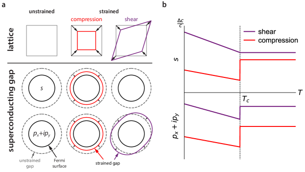
Figure 1: The influence of strain on one- and two-component superconductors. Panel (a) illustrates how two representative order parameters—single-component $s$-wave and two-component $p_{x}+ip_{y}$—respond to both compression and shear strain. Both gaps respond under compression (whether increasing or decreasing in magnitude depends on microscopic details). Only the two-component gap, however, couples to shear strain—here we illustrate the “phase” mode (see Ghosh et al. [2] for more details). Panel (b) shows the expected changes in elastic moduli across $T_{\rm c}$ for one and two component order parameters. All superconductors have a discontinuity in their compressional moduli across $T_{\rm c}$, but only two-component superconductors have discontinuities in their shear moduli.

The natural way to distinguish between single-component and two-component order parameters is to apply strain. Single-component superconductors have a single degree of freedom that couples to compression strains—the superfluid density—producing a discontinuity in the compressional elastic moduli at $T_{\rm c}$ (see Figure 1). They, however, have no such discontinuity in their shear moduli because shear strains preserve volume and thus do not couple to superfluid density. Multi-component superconductors, on the other hand, have additional degrees of freedom: the relative orientation of the two order parameters, as well as their relative phase difference. These additional degrees of freedom couple to shear strains, producing discontinuities in the shear moduli at $T_{\rm c}$. By identifying which elastic moduli have discontinuities at $T_{\rm c}$, one can determine whether a superconductor is multi-component without any microscopic knowledge of the Fermi surface or the pairing mechanism.

Dimensionality	Representation	Shear discontinuity?	Reference (E: experiment; T: theory)
One-Component	$A_{u}$	No	E: NMR [20]
			E: scanning SQUID [21]
	$B_{2u}$	No	E: Ultrasound (this work)
	$B_{3u}$	No	T: DFT [22]
			E: NMR[23, 24]
			E: scanning SQUID [21]
		No	E: specific heat [16, 17]
			E: uniaxial stress [25]
Two-Component	$\{B_{1u},A_{u}\}$	$c_{66}$	E: microwave surface impedance [15]
			E: specific heat, Kerr effect [12]
	$\{B_{3u},A_{u}\}$	$c_{44}$	E: penetration depth [8]
			E: NMR [26]
	$\{B_{1u},B_{2u}\}$	$c_{44}$	T: phenomenology analoguous to 3He [27, 28]
			E: specific heat [9]
	$\{B_{1u},B_{3u}\}$	$c_{55}$	T: phenomenology + DFT [29]
			T: DFT [30]
	$\{B_{2u},B_{3u}\}$	$c_{66}$	T: DFT [31, 32]
			E: specific heat, Kerr effect [12, 13]
			T: emergent $D_{4h}$ symmetry under RG flow [33]
		Yes	E: STM [14]
			T: pair-Kondo effect [34]
			T: MFT of Kondo lattice [35]

Table 1: Proposed order parameters for UTe₂. Proposed odd-parity order parameters for UTe₂, sorted by the number of components (dimensionality), their irreducible representation, and whether the proposed order parameter is based on an experimental observation or a theoretical proposal. Scenarios listed without a specific representation are compatible with any type of one or two-component order parameter. Based on symmetry alone, our work strongly constrains the order parameter to be of the one-component type. Using more quantitative arguments, we suggest a $B_{2u}$ order parameter.

II Results

We use a traditional phase-comparison pulse-echo ultrasound technique to measure the temperature dependence of six elastic moduli in three different samples of UTe₂ over a temperature range from about 1.3 K to 1.9 K. In particular, we measure all three compressional (i.e. $c_{11}$, $c_{22}$, and $c_{33}$) and shear (i.e. $c_{44}$, $c_{55}$, and $c_{66}$) moduli in one sample with two superconducting transitions (S3: $T_{c,1}\approx 1.64$ K, $T_{c,2}\approx 1.60$ K) and in two samples with a single $T_{\rm c}$ (S1: $T_{c}\approx 1.63$ K and S2: $T_{c}\approx 1.70$ K). Ultrasound data in the normal state of UTe₂ have been reported in Ushida et al. [36]. Here, we focus on the superconducting transition. Details of the sample growth and preparation, as well as the experiment, are given in the Methods.

Figure 2 shows the relative changes in four elastic moduli across $T_{\rm c}$ for the single-transition samples S1 and S2. We observe a single, sharp ($\approx$ 85 mK wide) discontinuity in the $c_{33}$ compressional modulus, as expected for all superconducting transitions. We observe no discontinuities in any of the shear elastic moduli to within our experimental resolution (a few parts in $10^{7}$, see S.I. for details).

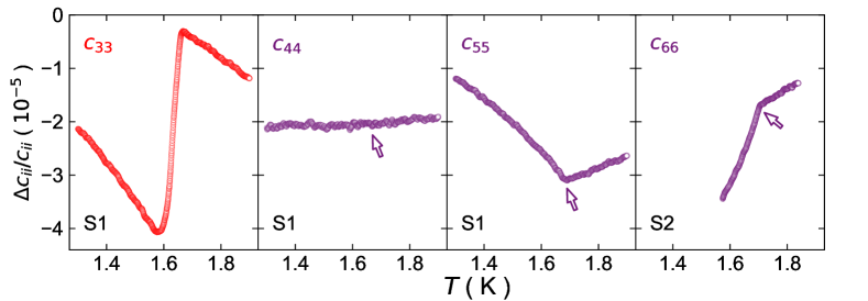
Figure 2: Relative change in elastic moduli through $T_{\rm c}$ for single-$T_{\rm c}$ UTe₂. A compressional elastic modulus, $c_{33}$, shows a sharp discontinuity of approximately 40 parts per million at $T_{\rm c}$, as expected for all superconductors. In contrast, the shear elastic moduli—$c_{44}$, $c_{55}$, and $c_{66}$—show only changes in slope at $T_{\rm c}$, consistent with a single-component superconducting order parameter. Empty arrows mark the superconducting transition for all shear moduli. $\Delta c_{ii}/c_{ii}$ is defined as $\left(c_{ii}(T)-c_{ii}(T_{0})\right)/c_{ii}(T_{0})$ where $T_{0}$ is the highest temperature in the plot.

Figure 3 shows the relative changes in the elastic moduli for sample S3 with a double superconducting transition (the single-$T_{\rm c}$ data is reproduced here for comparison). We observe two distinct discontinuities in $c_{33}$ separated by approximately 40 mK. Subsequent specific heat measurements on the same sample show a similar “double peak” feature identified in other double-$T_{\rm c}$ samples [12] (specific heat data is shown in the S.I.). Notably, we find the sum of the discontinuities in the double-$T_{\rm c}$ sample to be of a similar size as the discontinuity in the single-$T_{\rm c}$ sample. Additionally, the behaviour of the shear elastic moduli is nearly identical to that of the single-$T_{\rm c}$ samples, again with no discontinuities at $T_{\rm c}$.

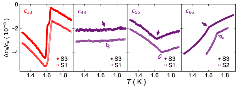
Figure 3: Relative change in elastic moduli through $T_{\rm c}$ for double-$T_{\rm c}$ UTe₂. The compressional elastic modulus $c_{33}$ shows two distinct discontinuities at $T_{\rm c}$, consistent with the two peaks we find in the specific heat of the same sample. The shear moduli, on the other hand, show no discontinuities and behave nearly identically to the shear moduli of the single-$T_{\rm c}$ sample. Single (double) transition samples are shown with empty (filled) symbols. Empty (filled) arrows mark the superconducting transition for all shear moduli for single (double) transition samples. $\Delta c_{ii}/c_{ii}$ is defined as in Figure 2, and curves have been offset for clarity.

We also measure the two other compressional moduli—$c_{11}$ and $c_{22}$—and show them along with $c_{33}$ in Figure 4. $c_{11}$ has a discontinuity of approximately 20 parts per million—roughly a factor of 2 smaller than the discontinuity in $c_{33}$. In contrast, $c_{22}$ has a discontinuity of at most 1 part per million—significantly smaller than the other two compressional moduli. Discontinuities in all three compressional moduli are allowed by symmetry for any superconducting order parameter (see Ghosh et al. [2] and the S.I.).

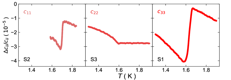
Figure 4: Relative change in compressional elastic moduli through $T_{\rm c}$. The compressional elastic moduli are shown as a function of temperature through $T_{\rm c}$. $c_{33}$ and $c_{11}$ were measured on a single-$T_{\rm c}$ sample and $c_{22}$ was measured on the double-$T_{\rm c}$ sample. Both $c_{11}$ and $c_{33}$ have clearly resolvable discontinuities at $T_{\rm c}$, whereas $c_{22}$ has a barely-resolvable discontinuity. $\Delta c_{ii}/c_{ii}$ is defined as in Figure 2.

We first analyze the data using only the presence or absence of discontinuities in the elastic moduli. This analysis is based on symmetry arguments alone and is independent of the size of the discontinuities. We then perform a quantitative analysis of the discontinuities using Ehrenfest relations. Finally, we combine all of our observations to speculate on which particular superconducting order parameter is most consistent with our data.

Symmetry of the superconducting order parameter. The presence or absence of a discontinuity in each elastic modulus constrains the symmetry of the superconducting order parameter. Roughly speaking, only strains that couple linearly to a degree of freedom associated with the superconducting order parameter show discontinuities at $T_{\rm c}$. We illustrate this with a couple of examples; a more rigorous derivation is given in the SI.

Discontinuities in elastic moduli arise when there is coupling between strain and superconductivity that is linear in strain and quadratic in the order parameter. For a single-component superconducting order parameter, this only occurs for compression strains [37]. A single-component order parameter can be written as $\eta=\eta_{0}e^{i\phi}$, where $\eta_{0}$ is the magnitude of the gap (which may depend on momentum) and $\phi$ is the superconducting phase. The lowest-order coupling to a strain $\epsilon_{ij}$ is $\epsilon_{ij}\eta^{\star}\eta=\epsilon_{ij}\eta_{0}^{2}$, where $(^{\star})$ denotes complex conjugation. This coupling is allowed only if $\epsilon_{ij}$ preserves the symmetry of the lattice, i.e. it is only allowed for compression strains and not for shear strains (which break the lattice symmetry). Since $\eta_{0}^{2}$ is proportional to the superfluid density, the physical interpretation of the resulting discontinuity at $T_{\rm c}$ is that compression strain couples to the superfluid density, which turns on at $T_{\rm c}$ and provides a new degree of freedom that softens the lattice.

In contrast to single-component order parameters, multi-component order parameters can have discontinuities in shear elastic moduli. This is because there are more degrees of freedom associated with a multi-component order parameter than with a single-component order parameter. Writing a two-component order parameter as $\vec{\eta}=\left\{\eta_{0,i}e^{i\phi_{i}},\eta_{0,j}e^{i\phi_{j}}\right\}$, there are now several possible couplings at lowest order. Taking the well-known $p$-wave state in tetragonal crystals as an example, one possible coupling is $\epsilon_{xy}\eta_{0,p_{x}}\eta_{0,p_{y}}\cos\left(\phi_{x}-\phi_{y}\right)$ . This is the so-called “phase mode” of the order parameter, as it couples shear $xy$ strain to the relative phase of the two components (see Figure 1). This produces a discontinuity in the associated elastic modulus $c_{66}$. The relative phase is a new degree of freedom that is only present in a multicomponent order parameter, as strain cannot couple to the absolute phase of a single-component order parameter (such a term would break gauge symmetry). Similar expressions exist for orthorhombic crystals (see SI for details), but the main conclusion is independent of the crystal structure: shear elastic moduli only exhibit discontinuities at $T_{\rm c}$ for multi-component superconducting order parameters.

The absence of a discontinuity in any shear elastic modulus in the single-transition samples (S1 and S2) rules out all uniform-parity , two-component order parameters in UTe₂. While there are no natural two-component order parameters in UTe₂ because the crystal structure is orthorhombic, many nearly or accidentally-degenerate order parameters have been proposed to explain the presence of the two nearly-degenerate $T_{\rm c}$’s, time reversal symmetry breaking, and chiral surface states (see Table 1). One proposal is the onset of first a B_2u state followed by a B_3u state at the second, lower $T_{\rm c}$ [12, 13, 31, 32, 33]. This proposal predicts the usual discontinuities in compressional moduli at the first (higher-temperature) $T_{\rm c}$, followed by a discontinuity in the compressional moduli and the $c_{66}$ shear modulus at the lower $T_{\rm c}$. In fact, the product of any two odd-parity (i.e. $p$ or $f$-wave) states or any two even-parity states (i.e. $s$ or $d$-wave) in D_2h predicts a discontinuity in either $c_{44}$, $c_{55}$, or $c_{66}$, none of which we observe. This strongly constrains the superconducting order parameter of UTe₂ to be of the single-component type. Finally, we note that our data is fully consistent with any single-component order parameter, including even-parity states like $s$-wave and $d$-wave.

The similar absence of discontinuities in the shear elastic moduli of the two-transition sample (S3) rules out the multi-component explanation for the second superconducting transition. We find that the single discontinuity in $c_{33}$ in single-$T_{\rm c}$ samples is approximately the same size as the sum of the two discontinuities found in double-$T_{\rm c}$ samples. This suggests that, below the second transition, all electrons in UTe₂ are in the same thermodynamic state, rather than double-$T_{\rm c}$ samples having two separate superconducting mechanisms. This suggests a common origin for the two superconducting transitions, perhaps split by local strains [17] or magnetic impurities [40]. Why this usually manifests as only two sharp $T_{\rm c}$’s (as we also observe in our data), rather than multiple $T_{\rm c}$’s or a broad transition, remains an open question. It also leaves unresolved the issue of why even single-$T_{\rm c}$ samples become double-$T_{\rm c}$ samples under hydrostatic pressure, leaving open the possibility of the appearance of a multi-component order parameter under pressure.

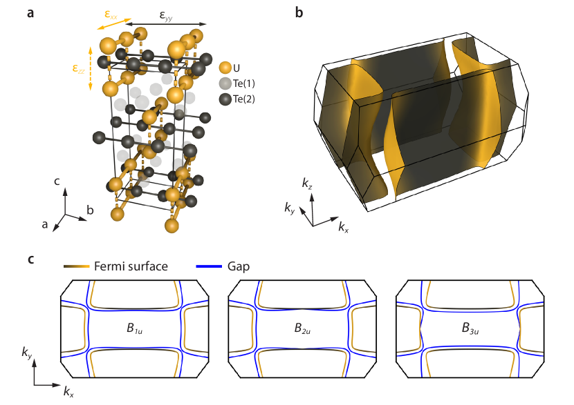
Figure 5: Influence of compression strains on the crystal structure and Fermi surface of UTe₂. Panel (a) shows the crystal structure of UTe₂. Highlighted are tellurium chains along the $b$ axis, and chains that run along the $a$ axis consisting of $c$-axis-oriented uranium dimers. These chains dominate the geometry of the Fermi surface shown in panel (b), modeled after quantum oscillation measurements [41]. The Fermi surface is colored according to its uranium (yellow) and tellurium (gray) content. The superconducting gaps for three possible odd-parity order parameters are shown at $k_{z}=0$ as blue lines in panel (c).

Ehrenfest analysis and the coupling of compression strains to superconductivity. The smallness of the discontinuity in $c_{22}$ compared to the other two compressional moduli indicates that the superconductivity in UTe₂ is insensitive to strain along the $b$ axis ($\epsilon_{yy}$). This observation is made quantitative through Ehrenfest relations, which relate discontinuities in the elastic moduli, $\delta c_{ij}$, to the discontinuity in the specific heat, $\Delta C$. The Ehrenfest relations are

$$\delta c_{ij}=-\frac{\Delta C}{T}\left(\frac{dT_{\rm c}}{d\epsilon_{ij}}\right)^{2},$$ (1)

where $\frac{dT_{\rm c}}{d\epsilon_{ij}}$ is the derivative taken at zero applied stress. Using the specific heat measured on sample S3 (see S.I.) and the data shown in Figure 4, we calculate $\frac{dT_{\rm c}}{d\epsilon_{xx}}=0.23\pm 0.02$ K/(% strain), $\frac{dT_{\rm c}}{d\epsilon_{yy}}=0.07\pm 0.02$ K/(% strain), and $\frac{dT_{\rm c}}{d\epsilon_{zz}}=0.34\pm 0.02$ K/(% strain). These values are roughly consistent with those measured in uniaxial strain experiments [25] (see S.I. for the quantitative comparison).

These Ehrenfest relations indicate that the superconductivity of UTe₂ is significantly more sensitive to strains along the $a$ and $c$ axes than it is to strain along the $b$ axis. This observation is perhaps surprising given the relatively quasi-two-dimensional nature of the Fermi surface measured by quantum oscillations in UTe₂ [41, 42]. The Fermi surface consists of two sets of quasi-one-dimensional sheets running along the $a$ and $b$ axes that hybridize to form one electron and one hole pocket (see Figure 5). Thus, if any direction is to be weakly coupled to superconductivity, one might expect it to be the $c$ axis. This argument is unchanged by the possible existence of an additional small pocket of Fermi surface reported by Broyles et al. [43], as it is roughly isotropic and thus does not single out any particular direction.

Looking at the crystal structure in Figure 5, however, it is clear that the $a$ and $b$ axes are highly asymmetric: chains of $c$-axis-coupled uranium dimers run along the $a$ axis, whereas chains of tellurium run along the $b$ axis (the other tellurium site, Te(1), participates much less in the Fermi surface than the Te(2) chains: see SI.). Thus $\epsilon_{xx}$ and $\epsilon_{zz}$ modulate the inter and intra-dimer coupling of the uranium dimers, respectively, whereas $\epsilon_{yy}$ only modulates the weak inter-chain coupling of the uranium chains. $\epsilon_{yy}$ does, however, modulate the intra-chain spacing of tellurium chains along the $b$ axis. Our observation of the relative insensitivity of $T_{\rm c}$ to $\epsilon_{yy}$ therefore suggests that the superconducting pairing is more sensitive to the uranium-uranium distances than to the tellurium-tellurium distances.

Proposed single-component superconducting order parameter. Thermal transport [6], specific heat [7, 9], and penetration depth [8] all suggest the presence of point nodes in the superconducting gap of UTe₂. $B_{1u}$, $B_{2u}$, and $B_{3u}$ order parameters all have point nodes in their superconducting gaps, but these nodes lie along different directions in momentum space and thus intersect different portions of the Fermi surface (or may not intersect the Fermi surface at all if it is quasi-2D).

We use our observation of relatively weak coupling between $\epsilon_{yy}$ and $T_{\rm c}$ to motivate a particular orientation of the point nodes in UTe₂ and to suggest one particular single-component order parameter. Figure 5 shows a tight binding model of the Fermi surface of UTe₂ as determined by quantum oscillations, color-coded by the relative uranium 6$d$ and tellurium 5$p$ content (both bands have significant uranium 5$f$ character that contribute to their heavy masses, but not to their geometry). Our results suggest that the superconducting gap is either weak or absent on the tellurium-dominant electron Fermi surface. Only the $B_{2u}$ order parameter has nodes that lie along the $k_{y}$ direction, producing a node in the gap on the tellurium-dominant surface and a gap maximum on the uranium-dominant surface. We note that a reported small pocket with a light mass does not qualitatively affect this argument [43], as it is largely isotropic in shape and thus will not respond differently to $\epsilon_{xx}$ and $\epsilon_{yy}$ strain.

III Discussion

Our primary result is that the superconducting transitions in both single and double-transition samples of UTe₂ exhibit no thermodynamic discontinuities in any of the shear elastic moduli at $T_{\rm c}$. The strictest interpretation of this result is that it rules out all multi-component order parameters that have a bilinear coupling to strain. For UTe₂, this rules out all multi-component order parameter scenarios except for mixed-parity order parameters like $s$ + $p$ wave .

Looking beyond our own experiment, there is strong evidence that UTe₂ has an odd-parity order parameter. There is also strong evidence for nodes in the superconducting gap. Combined with our result, this leaves the three $B_{iu}$ representations as the only possibilities. We argue that our observation of a lack of sensitivity of $T_{\rm c}$ to $\epsilon_{yy}$ suggests a $B_{2u}$ order parameter.

A single-component order parameter places constraints on possible explanations for other experiments. First, a single-component order parameter cannot break time reversal symmetry. This suggests that the interpretation of time reversal symmetry breaking at $T_{\rm c}$ as seen by polar Kerr effect measurements [12, 13], along with the chiral surface states seen in STM [14] and microwave surface impedance measurements [15], may need to be revisited.

The search for multi-component superconductors continues: they are of both fundamental and practical interest, since a multi-component order parameter is a straightforward route to topological superconductivity. We find that, while UTe₂ may have an odd-parity, spin-triplet order parameter, it seems that the most likely order parameter to condense at $T_{\rm c}$ is of the single-component $B_{2u}$ representation—either $p_{y}$ or $f_{yz^{2}}$-wave superconductivity. Definitive determination of the orientation of the nodes in the superconducting gap would confirm this scenario.

IV Methods

IV.1 Sample Growth and Preparation

Single crystals of UTe₂ were grown by the chemical vapor transport (CVT) method as described in Ran et al. [7, 44]. Samples with one $T_{\rm c}$ (two $T_{\rm c}$’s) were grown in a two-zone tube furnace with temperatures of $950^{\circ}$C and $860^{\circ}$C ($1060^{\circ}$C and $1000^{\circ}$C) at the hot and cold end, respectively.

Specimens were aligned to better than $1^{\circ}$ using their magnetic anisotropy (performed in a Quantum Design MPMS) and X-ray diffraction (performed in a Laue backscattering system) measurements. Samples were then polished to produce two parallel faces normal to the $(100)$, $(010)$, and $(001)$ directions, depending on the mode geometry (see Table 2).

Thin-film ZnO piezoelectric transducers were sputtered from a ZnO target in an atmosphere of oxygen and argon. Both shear and longitudinal responses are present in each transducer—the shear axis was aligned with either the $(100)$, $(010)$, or $(001)$, again depending on the particular mode geometry. 3 crystals were measured in total; see Table 2 for details. The shear response in our deposited transducers was achieved by mounting the sample on the far end of the sputtering sample stage, maximizing the distance between sample and ZnO target. The position of the sample stage was fixed during the entire deposition process (i.e. rotation was disabled on the sample stage). The resulting polarization direction of the generated sound wave is then parallel to the shortest line drawn between the sample and the target—this orientation was verified using the absolute speed of sound and the moduli obtained using resonant ultrasound spectroscopy [45].

# $T_{c}$	Sample	$\vec{k}$	$\vec{u}$	$c_{ij}$	$f$ (MHz)	$d$ ($\mu$m)	$c$ (GPa)
1	S1	$[001]$	$[100]$	$c_{55}$	1261	$330\pm 17$	$51\pm 5$
			$[010]$	$c_{44}$	1434	$330\pm 17$	$27\pm 3$
			$[001]$	$c_{33}$	2260	$330\pm 17$	$91\pm 11$
	S2	$[100]$	$[100]$	$c_{11}$	823	$920\pm 46$	$81\pm 8$
			$[010]$	$c_{66}$	1250	$920\pm 46$	$28\pm 3$
2	S3	$[001]$	$[100]$	$c_{55}$	1348	$550\pm 28$	$52\pm 5$
			$[010]$	$c_{44}$	1352	$550\pm 28$	$28\pm 3$
			$[001]$	$c_{33}$	1348	$550\pm 28$	$88\pm 9$
		$[010]$	$[100]$	$c_{66}$	1362	$290\pm 15$	$30\pm 3$
			$[010]$	$c_{22}$	1362	$290\pm 15$	$141\pm 15$

Table 2: Sample configuration. Listed are the transducer configurations for all the measurements in this manuscript. Samples are sorted by the number of superconducting phase transitions (first column). Additional information given is the propagation $\vec{k}$ and the polarization $\vec{u}$ of the sound pulse excited in the sample, as well as the measured elastic modulus. Also shown is the frequency at which each measurement is performed. We also provide the thicknesses $d$ of the measured samples and the resulting absolute values of the elastic moduli obtained from the separation of echoes at room temperature. Uncertainties represent a 5 % uncertainty on the thickness.

IV.2 Pulse-Echo Ultrasound Measurements

Measurements were performed in an Oxford Instruments Heliox ³He refrigerator. We used a traditional phase-comparison pulse-echo ultrasound method to measure the change in elastic moduli relative to the highest temperature $T_{0}$, i.e. we measured $\Delta c/c\equiv\left(c(T)-c(T_{0})\right)/c(T_{0})$. Short bursts (typically $\sim 50$ ns) of radiofrequency signals, with the carrier frequency between 500 MHz and 2.5 GHz, were generated with a Tektronix TSG 4106A RF generator modulated by a Tektronix AFG 31052 arbitrary function generator, amplified by a Mini-Circuits ZHL-42W+ power amplifier, and transmitted to the transducer. The signal was detected with the same transducer, amplified with a Mini-Circuits ZX60-3018G-S+ amplifier, and recorded on a Tektronix MSO64 oscilloscope. The detection amplifier was isolated from the power amplifier using Mini-Circuits ZFSWA2-63DR+ switches, timed with the same Tektronix AFG 31052 arbitrary function generator.

Both shear and compressional sound are generated by our transducers—these signals are separated in the time domain due to the different speeds of propagation and identified as shear or compression using the known elastic moduli of UTe₂ [45]. Figure 6 shows a raw pulse-echo signal from a transducer sputtered on sample S3 with sound propagating along the [010] direction with a shear polarization axis along [100], thus measuring $c_{22}$ and $c_{66}$ simultaneously. Echoes corresponding to the different elastic modes can be clearly identified as shear (red vertical dashed lines) and compression (blue vertical dashed lines).

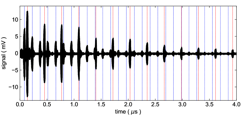
Figure 6: Raw Pulse-Echo Signal. The raw signal from a sputtered ZnO shear transducer on sample S3 with sound propagation along the [010] and polarization along the [100] directions. The transducer exhibits both a compressional (blue lines) and a shear (red dashed lines) response. These correspond to sound modes determined by the elastic moduli $c_{22}$ and $c_{66}$, respectively.

The phase of each echo was analyzed using a software lockin, and the relative change in phase between two echoes was converted to the relative change in speed of sound as a function of temperature. In Figure 7 we compare the temperature dependence of $c_{33}$ of samples S1 and S3 obtained with different transducers.

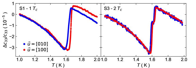
Figure 7: Transducer Comparison. Shown are $\Delta c_{33}/c_{33}$ for single $T_{\rm c}$ (S1, left) and two $T_{\rm c}$ (S3, right) samples. For each sample we compare the relative change in elastic modulus between measurements obtained with two different transducers. Both transducers excited sound along the [001] direction. However, for the data in red, the shear component of the transducer was polarized along [100] (additionally measuring $c_{55}$), whereas for the data in blue, the shear component of the transducer was polarized along [010] (additionally measuring $c_{44}$).

V Data Availability

Data that support the plots within this paper and other findings of this study are available from the corresponding author upon reasonable request.

VI Acknowledgments

We acknowledge helpful discussions with D. Agterberg and P. Brydon. B.J.R. and F.T. acknowledge funding from the Office of Basic Energy Sciences of the United States Department of Energy under award no. DE-SC0020143 for preparing the samples and transducers, performing the measurements, analyzing the data, and writing the manuscript. Research at the University of Maryland was supported by the Department of Energy award number DE-SC-0019154 (sample characterization), the Gordon and Betty Moore Foundation’s EPiQS Initiative through grant number GBMF9071 (materials synthesis), the National Science Foundation under grant number DMR-2105191 (sample preparation), the Maryland Quantum Materials Center and the National Institute of Standards and Technology. A part of this work was performed at the Cornell Center for Materials Research Shared Facilities which are supported through the NSF MRSEC program (DMR-1719875).

VII SUPPLEMENTARY INFORMATION

VII.1 Data Reproducibility

Figure 8 and Figure 9 show the relative change of elastic moduli as a function of temperature as obtained when different echoes from a single experiment are used for the data analysis. Figure 10 and Figure 11 show the relative change of elastic moduli for different carrier frequencies of the excited sound pulse. We find no significant dependence on either the echoes, or the frequencies used for any of our measurements.

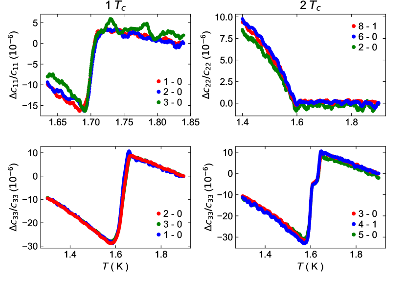
Figure 8: Echo Analysis Compressional Moduli. The relative change of compressional elastic moduli as obtained from different echoes in a single pulse-echo ultrasound experiment. The colors indicate the echoes used for each curve. The data in red are the data shown in the main. The left column shows data for samples with one superconducting transition, the right column is for samples with two transitions.

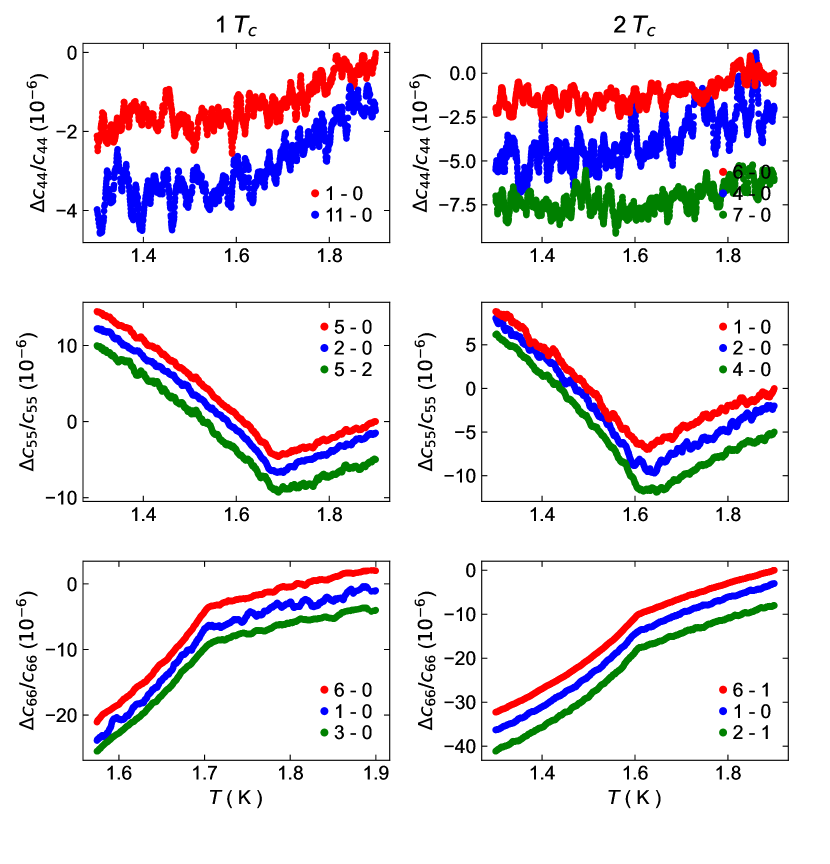
Figure 9: Echo Analysis Shear Moduli. The relative change of shear elastic moduli as obtained from different echoes in a single pulse-echo ultrasound experiment. The colors indicate the echoes used for each curve. The data in red are the data shown in the main. The left column shows data for samples with one superconducting transition, the right column is for samples with two transitions.

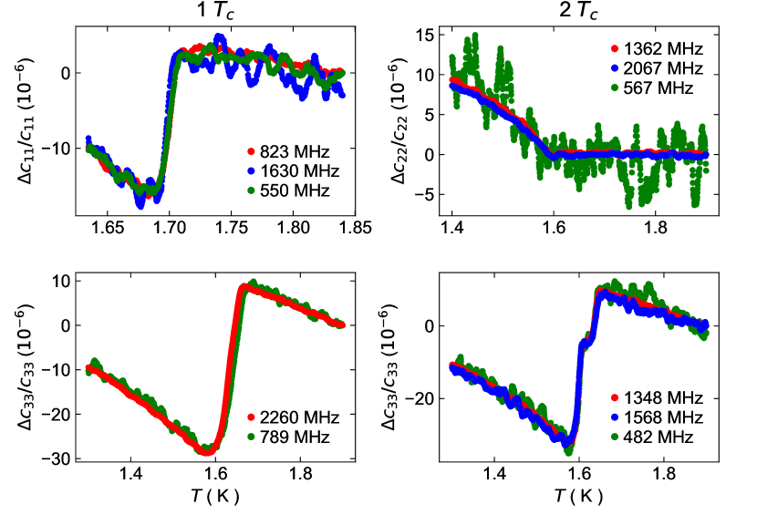
Figure 10: Frequency Dependence Compressional Moduli. The relative change of compressional elastic moduli at different frequencies. The data in red are the data shown in the main. The left column shows data for samples with one superconducting transition, the right column is for samples with two transitions.

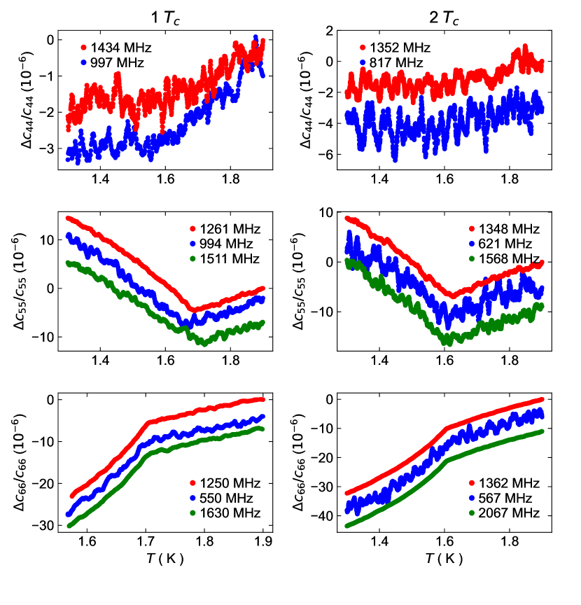
Figure 11: Frequency Dependence Shear Moduli. The relative change of shear elastic moduli at different frequencies. The data in red are the data shown in the main. The left column shows data for samples with one superconducting transition, the right column is for samples with two transitions.

VII.2 Noise Analysis

Figure 12 shows the relative change of all elastic moduli also shown in the main. In order to estimate the noise of our data, a second order polynomial has been fitted to the normal state data (highlighted by a red background in Figure 12). In Figure 13 we show the same elastic moduli with that polynomial subtracted from the data. We then estimate its noise as the RMS of the background-subtracted data above the transition, i.e. the same temperature range which we used to fit said polynomial background (red shaded region). The resulting RMS values lie between 0.04 ppm and 0.41 ppm (on average less than $1.9\times 10^{-7}$).

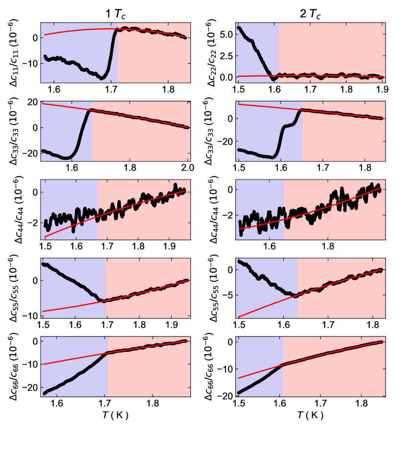
Figure 12: Background Subtraction. Temperature dependence of all elastic moduli shown in the main (black points). A second order polynomial (red line) has been fitted to each modulus in the normal state above $T_{c}$ (red shaded region). The left column shows data for samples with one superconducting transition, the right column is for samples with two transitions.

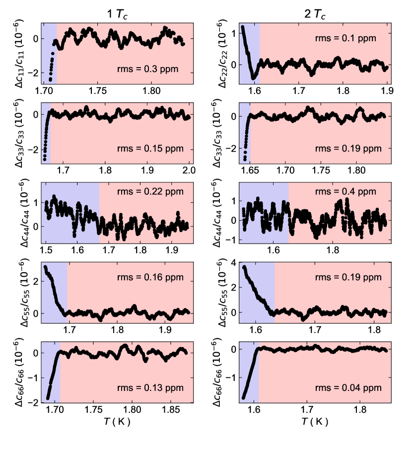
Figure 13: Noise Estimate. Elastic moduli from Figure 12 with the normal state background (see Figure 12) subtracted. A RMS is calculated for each modulus in the same temperature range that was used to fit the background in Figure 12 (red shaded region). The purple/red shaded temperature regions are identical to those in Figure 12. The left column shows data for samples with one superconducting transition, the right column is for samples with two transitions.

VII.3 Landau Free Energy Calculations

Elastic moduli are the second derivative of the free energy with respect to strain, i.e. they are the strain susceptibility, in analogy with the heat capacity, which is the second derivative of the free energy with respect to temperature. If strain couples linearly to the square of the order parameter $\eta$ (just like temperature does in the term $(T-T_{c})\eta^{2}$), the respective elastic modulus will exhibit a discontinuity at the phase transition (just like the specific heat does). The reason for these discontinuities is that immediately below $T_{c}$, the system has a new degree of freedom that can respond when you apply strain (in the case of elastic moduli) or change temperature (in the case of heat capacity). This new degree of freedom means that the response below $T_{c}$ is entirely distinct from that above $T_{c}$: even though the order parameter itself changes continuously, the system’s susceptibility to changes in the order parameter is discontinuous.

For a single-component order parameter, only compressional moduli can exhibit this discontinuity. For a two-component order parameter, on the other hand, discontinuities in compressional moduli and certain shear moduli are allowed. This is because for single-component order parameters, the only quantity that can respond to strain is the magnitude of the order parameter. The bare “amplitude” of the order parameter breaks gauge symmetry and thus cannot enter directly into the free energy or couple linearly to external parameters like strain. As the magnitude of the order parameter is a scalar (simply a number), this means that it couples to scalar strains, i.e. compressional moduli.

For a two component order parameter, there are two new gauge-invariant quantities that can couple to strain: the relative phase between the components of the order parameter, and the overall “orientation” of the two components in order-parameter space. These are new degrees of freedom that can be probed by shear strain, and thus are what allow for discontinuities in the shear moduli at $T_{c}$.

Below, we elaborate on these concepts within the Landau theory of second-order phase transitions.

VII.3.1 Elastic Free Energy

The elastic free energy of a solid is given by $\frac{1}{2}\sum_{i,j}\varepsilon_{i}c_{ij}\varepsilon_{j}$, with strain $\vec{\varepsilon}=\{\varepsilon_{xx},\varepsilon_{yy},\varepsilon_{zz},2\varepsilon_{yz},2\varepsilon_{xz},2\varepsilon_{xy}\}$ and the elastic tensor $\boldsymbol{c}$ in Voigt notation. In an orthorhombic crystal environment (i.e. point group $D_{2h}$), all individual elements of the strain tensor transform as a particular irreducible representation of the point group $D_{2h}$. In particular, we can rewrite

$$\vec{\varepsilon}=\{\varepsilon_{xx},\varepsilon_{yy},\varepsilon_{zz},2\varepsilon_{yz},2\varepsilon_{xz},2\varepsilon_{xy}\}=\{\varepsilon_{Ag,1},\varepsilon_{Ag,2},\varepsilon_{Ag,3},\varepsilon_{B3g},\varepsilon_{B2g},\varepsilon_{B1g}\},$$ (2)

where the subscript now refers to the irreducible representation. Consequently, the elastic free energy can be rewritten as

$$f_{el}= \frac{1}{2}\left(c_{Ag,1}\varepsilon_{Ag,1}^{2}+c_{Ag,2}\varepsilon_{Ag,2}^{2}+c_{Ag,3}\varepsilon_{Ag,3}^{2}+2c_{Ag,4}\varepsilon_{Ag,1}\varepsilon_{Ag,2}+2c_{Ag,5}\varepsilon_{Ag,1}\varepsilon_{Ag,3}+2c_{Ag,6}\varepsilon_{Ag,2}\varepsilon_{Ag,3}\right.$$ (3)

$$\left.+c_{B3g}\varepsilon_{B3g}^{2}+c_{B2g}\varepsilon_{B2g}^{2}+c_{B2g}\varepsilon_{B2g}^{2}\right).$$

Here, we have rewritten the elastic tensor according to

$$\boldsymbol{c}=\begin{pmatrix}c_{11}&c_{12}&c_{13}&0&0&0\\ c_{12}&c_{22}&c_{23}&0&0&0\\ c_{13}&c_{23}&c_{33}&0&0&0\\ 0&0&0&c_{44}&0&0\\ 0&0&0&0&c_{55}&0\\ 0&0&0&0&0&c_{66}\\ \end{pmatrix}=\begin{pmatrix}c_{Ag,1}&c_{Ag,4}&c_{Ag,5}&0&0&0\\ c_{Ag,4}&c_{Ag,2}&c_{Ag,6}&0&0&0\\ c_{Ag,5}&c_{Ag,6}&c_{Ag,3}&0&0&0\\ 0&0&0&c_{B3g}&0&0\\ 0&0&0&0&c_{B2g}&0\\ 0&0&0&0&0&c_{B1g}\\ \end{pmatrix}.$$ (4)

VII.3.2 Order Parameter Free Energy and Coupling to Strain:
One-Component Order Parameter

A single-component superconducting order parameter (OP) can be parametrized as $\eta e^{i\gamma}$, with an amplitude $\eta$ and phase $\gamma$, both real. However, since the free energy needs to obey global gauge symmetry, the OP can only appear in even powers and the phase factor $e^{i\gamma}$ becomes unobservable. Only one degree of freedom remains, the amplitude (or superfluid density) $\eta$. The phase factor is thus dropped in the following discussion. In this case, the OP free energy expansion to fourth order reads

$$f_{OP}=\frac{a}{2}\eta^{2}+\frac{b}{4}\eta^{4},$$ (5)

where $a=a_{0}\left(T-T_{c}\right)$. $a_{0}>0$, and $b$ are phenomenological constants, $T_{c}$ is the critical temperature.

Since the OP has to appear in even powers in the free energy, the lowest possible coupling to strain is quadratic in OP and linear in strain. Furthermore, since the OP transforms as a one-dimensional irreducible representation of $D_{2h}$, its bilinear will always transform as the $A_{g}$ irreducible representation, irrespective of the particular representation. Thus, quadratic in OP and linear in strain coupling terms are only allowed for $A_{g}$ strains, and to lowest order, the terms in the free energy coupling the OP to strain are

$$f_{coupling}=\frac{1}{2}\left(g_{1}\varepsilon_{Ag,1}+g_{2}\varepsilon_{Ag,2}+g_{3}\varepsilon_{Ag,3}\right)\eta^{2}.$$ (6)

Following the formalism outlined in [2], coupling of strain to the OP leads to a discontinuity of the respective elastic moduli at $T_{c}$ according to

$$\delta c_{mn}=\left.-\frac{Z_{m}Z_{n}}{Y}\right|_{\eta\rightarrow\eta_{0},\varepsilon_{m}\rightarrow 0},$$ (7)

where $Z_{m}=\frac{\partial^{2}f_{coupling}}{\partial\eta\partial\varepsilon_{m}}$, $Y=\frac{\partial^{2}f_{OP}}{\partial\eta^{2}}$, and $\eta_{0}=\sqrt{\frac{-a}{b}}$ is the equilibrium value for the OP defined by $\partial f_{OP}/\partial\eta=0$. From Equation 7 it is straightforward to see that coupling terms in the free energy which are quadratic or higher order in strain will not lead to a discontinuity of the respective elastic modulus at $T_{c}$, which justifies the truncation of Equation 6 after terms linear in strain. Consequently, in the case of a one-component OP, no shear modulus (i.e. $c_{B1g}$, $c_{B2g}$, or $c_{B3g}$) is allowed to show a discontinuity at $T_{c}$ (note that a discontinuity in its derivative is allowed [46]). This is a general statement purely based on the dimensionality of the order parameter and irrespective of its particular irreducible representation. Combining Equation 6 and Equation 7, all $A_{g}$ elastic moduli exhibit a discontinuity at the critical temperature. The magnitudes of these discontinuities based on the free energy in Equation 5 and Equation 6 are summarized in Table 3.

	One-Component OP	$B_{2u}+iB_{3u}$
	$\eta_{0}=\sqrt{\frac{-a}{b}}$	$\left(\theta_{0},\gamma_{0}\right)=\left(\pi/4,\pm\pi/2\right)$
		$\eta_{0}=\pm\sqrt{\frac{-2a_{1}}{b_{1}+b_{3}-b_{4}}}$
$\delta c_{Ag,i}$	$-\frac{g_{i}^{2}}{2b}\left(\eta\right)$	$\frac{a_{1}(-2a_{2}(b_{1}+b_{3}-b_{4})g_{i}^{a}g_{i}^{s}+a_{1}(-(b_{1}+b_{3}-b_{4})(g_{i}^{a})^{2}+4b_{2}g_{i}^{a}g_{i}^{s}-(b_{1}-b_{3}+b_{4})(g_{i}^{s})^{2}))}{a_{1}^{2}(b_{1}^{2}-4b_{2}^{2}-(b_{3}-b_{4})^{2})+4a_{1}a_{2}b_{2}(b_{1}+b_{3}-b_{4})-a_{2}^{2}(b_{1}+b_{3}-b_{4})^{2}}\left(\eta,\theta\right)$
$\delta c_{B1g}$	0	$-\frac{g_{4}^{2}}{2b_{4}}\left(\gamma\right)$
$\delta c_{B2g}$	0	0
$\delta c_{B3g}$	0	0

Table 3: Discontinuities in elastic moduli for different OP configurations. Magnitudes of discontinuities in elastic moduli at $T_{c}$ for one and two-component OPs, along with the particular degree of freedom that causes the discontinuity (given in parentheses after the expression for the discontinuity). For a one-component OP, only compressional moduli $c_{A_{g},i}$ show a discontinuity, caused by fluctuations in the order parameter amplitude $\eta$. For a $B_{2u}+iB_{3u}$ two-component OP, compressional moduli and the $c_{B1g}$ elastic modulus are allowed to show a discontinuity. The discontinuity in the compressional moduli is due to fluctuations in the absolute amplitdue $\eta$ of the OP, as well as fluctuations in the relative amplitude $\theta$ between individual components. The discontinuity in $c_{B1g}$, however, is caused by fluctuations of the relative phase $\gamma$ between different order parameter components.

VII.3.3 Order Parameter Free Energy and Coupling to Strain:
Two-Component Order Parameter

Next we discuss discontinuities in the elastic moduli with a two-component OP $\boldsymbol{\eta}=\{\eta_{x},\eta_{y}\}$. In the $D_{2h}$ point group, all irreducible representations are one dimensional. A two-component order parameter therefore has to consist of two one-component order parameters, meaning $\eta_{x}$ and $\eta_{y}$ can belong to different irreducible representations and are not related by symmetry. The example of $\eta_{x}$ and $\eta_{y}$ transforming as the $B_{2u}$ and $B_{3u}$ irreducible representations, respectively, as suggested for the superconducting OP in UTe₂ by authors in Hayes et al. [12] and Wei et al. [13], will be used in the discussion below. For this particular OP, three independent bilinear combinations can be formed: $\left|\eta_{x}\right|^{2}$, $\left|\eta_{y}\right|^{2}$, and $\left(\eta_{x}\eta_{y}^{*}+\eta_{x}^{*}\eta_{y}\right)$ transforming as $A_{g}$, $A_{g}$, and $B_{1g}$ representations respectively. The Landau free energy reads

$$f_{OP} =\frac{a_{1}}{2}\left(\left|\eta_{x}\right|^{2}+\left|\eta_{y}\right|^{2}\right)+\frac{a_{2}}{2}\left(\left|\eta_{x}\right|^{2}-\left|\eta_{y}\right|^{2}\right)$$ (8)

$$+\frac{b_{1}}{4}\left(\left|\eta_{x}\right|^{4}+\left|\eta_{y}\right|^{4}\right)+\frac{b_{2}}{4}\left(\left|\eta_{x}\right|^{4}-\left|\eta_{y}\right|^{4}\right)+\frac{b_{3}}{2}\left|\eta_{x}\right|^{2}\left|\eta_{y}\right|^{2}+\frac{b_{4}}{4}\left(\left(\eta_{x}\eta_{y}^{*}\right)^{2}+\left(\eta_{x}^{*}\eta_{y}\right)^{2}\right),$$

where $a_{1,2}=a_{1,2}^{(0)}\left(T-T_{c}\right)$, $a_{1,2}>0$, and $b_{i}$ are phenomenological constants. Based on these considerations, the free energy coupling the OP to linear powers of strain can be written as

$$f_{coupling} =\frac{1}{2}\left(g_{1}^{s}\varepsilon_{Ag,1}+g_{2}^{s}\varepsilon_{Ag,2}+g_{3}^{s}\varepsilon_{Ag,3}\right)\left(\left|\eta_{x}\right|^{2}+\left|\eta_{y}\right|^{2}\right)+\frac{1}{2}\left(g_{1}^{a}\varepsilon_{Ag,1}+g_{2}^{a}\varepsilon_{Ag,2}+g_{3}^{a}\varepsilon_{Ag,3}\right)]\left(\left|\eta_{x}\right|^{2}-\left|\eta_{y}\right|^{2}\right)$$ (9)

$$+\frac{g_{4}}{2}\varepsilon_{B1g}\left(\eta_{x}\eta_{y}^{*}+\eta_{x}^{*}\eta_{y}\right).$$

Coupling of $B_{1g}$ strain to the second power of the OP as in the free energy above is only possible for the particular example of a $\{B_{2u},B_{3u}\}$ OP. However, linear coupling of shear strain (i.e. $B_{1g}$, $B_{2g}$, or $B_{3g}$ strain in $D_{2h}$) to a bilinear of the OP is in general only possible for a two-component OP.

In order to calculate the discontinuities of elastic moduli in the presence of a two-component OP, Ghosh et al. [2] generalized the expression in Equation 7 to

$$\delta c_{mn}=\left.-\boldsymbol{Z}_{m}^{T}\boldsymbol{Y}^{-1}\boldsymbol{Z}_{n}\right|_{\boldsymbol{\eta}\rightarrow\boldsymbol{\eta}_{0},\varepsilon_{m}\rightarrow 0},$$ (10)

where $\boldsymbol{Z}_{m}=\frac{\partial^{2}f_{coupling}}{\partial\boldsymbol{\eta}\partial\varepsilon_{m}}$ and $\boldsymbol{Y}=\frac{\partial^{2}f_{OP}}{\partial\boldsymbol{\eta}^{2}}$. Parametrizing the OP as $\boldsymbol{\eta}=\eta\left\{\cos\theta,e^{i\gamma}\sin\theta\right\}$, the derivative $\partial/\partial\boldsymbol{\eta}$ becomes $\partial/\partial\left\{\eta,\theta,\gamma\right\}$. Assuming a chiral order parameter $\left(\theta_{0},\gamma_{0}\right)=\left(\pi/4,\pm\pi/2\right)$, the equilibrium amplitude $\eta_{0}$, defined by $\left.\partial f_{OP}/\partial\eta\right|_{\eta_{0},\theta_{0},\gamma_{0}}=0$, is then given by $\eta_{0}=\pm\sqrt{\frac{-2a_{1}}{b_{1}+b_{3}-b_{4}}}$. This assumption is motivated by the observation of time-reversal symmetry breaking (TRSB) [12, 13] in the superconducting state of UTe₂. For this order parameter configuration, one finds

$$\boldsymbol{Y}=\begin{pmatrix}a_{1}+\frac{3\eta_{0}^{2}}{2}\left(b_{1}+b_{3}-b_{4}\right)&-2\eta_{0}\left(a_{2}+b_{2}\eta_{0}^{2}\right)&0\\ -2\eta_{0}\left(a_{2}+b_{2}\eta_{0}^{2}\right)&\left(b_{1}-b_{3}+b_{4}\right)\eta_{0}^{4}&0\\ 0&0&\frac{b_{4}\eta_{0}^{4}}{2}\\ \end{pmatrix},$$ (11)

$$\boldsymbol{Z}_{Ag,i}=\begin{pmatrix}g_{i}^{s}\eta_{0}\\ -g_{i}^{a}\eta_{0}^{2}\\ 0\\ \end{pmatrix},~{}\boldsymbol{Z}_{B1g}=\begin{pmatrix}0\\ 0\\ -\frac{g_{4}\eta_{0}^{2}}{2}\\ \end{pmatrix},~{}\boldsymbol{Z}_{B2(3)g}=\begin{pmatrix}0\\ 0\\ 0\\ \end{pmatrix},$$ (12)

where $i=1,2,3$. From Equation 11 and Equation 12 in can be seen that for a chiral $\left\{B_{2u},B_{3u}\right\}$ order parameter in a $D_{2h}$ point group, all compressional moduli (i.e. the elastic moduli corresponding to $A_{g}$ strains) show a step discontinuity at $T_{c}$ due to coupling of the corresponding strain to the absolute amplitude of the OP (the superfluid density), as well as the relative amplitude of the different components (this is in contrast to a multi-component OP where the different components are related by symmetry, for which compressional strains only couple to the absolute amplitude of the OP [2]). Among all the shear moduli, only $c_{B1g}$ shows a step discontinuity at $T_{c}$, due to the coupling of $B_{1g}$ shear strain to the relative phase between the different components of the OP.

While the details of the above calculation depend on the exact OP parameter configuration, the main statement is general: a multi-component OP is required for a discontinuity in any shear modulus.

VII.4 Heat Capacity Measurements

Heat capacity measurements (Figure 14) were performed in a ³He cryostat using the quasi-adiabatic method: a fixed power was applied to the calorimeter to raise it approximately 1% over the bath temperature. The power was then turned off to allow the calorimeter to relax back to the bath temperature. The heat capacity was extracted from these heating and cooling data by fitting them to exponentially-saturating curves. The sample was affixed to the calorimeter with Apiezon N grease. The background heat capacity of the grease and the calorimeter were measured separately and subtracted from the data in Figure 14.

VII.5 Ehrenfest Analysis

The discontinuity observed in the compressional moduli $\delta c_{ii}$ at $T_{c}$ is directly related to the jump in the heat capacity divided by temperature, $\Delta C/T$, via Ehrenfest relations. For a single component order parameter they read

$$\delta c_{ii}=-\frac{\Delta C}{T}\left(\frac{dT_{c}}{d\varepsilon_{ii}}\right)^{2}.$$ (13)

The derivative of critical temperature with respect to compressional strain $dT_{c}/d\varepsilon_{ii}$ can therefore be calculated by extracting the discontinuities of the corresponding elastic modulus and the heat capacity at $T_{c}$. The heat capacity was measured in sample S3 (see Figure 14) and the size of its discontinuity at $T_{c}$ is determined to be $(196\pm 18)$ mJ/(mol K²). The magnitudes of the discontinuities in $\Delta c/c$ for all compressional moduli are extracted according to Figure 15 and the values are given in Table 4. Using these values, as well as the elastic moduli of UTe₂ [45], the absolute values of $dT_{c}/d\varepsilon_{ii}$ ($ii=xx,yy,zz$) are calculated (see Table 4).

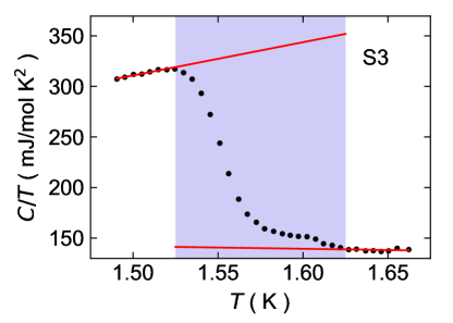
Figure 14: Heat Capacity. Heat capacity divided by temperature as a function of temperature measured on sample S3. The jump at $T_{c}$ is $(196\pm 18)$ mJ/(mol K²), determined according to linear fits below and above the transition (red lines). The uncertainty is estimated from the finite temperature range close to $T_{c}$ in which the data deviates significantly from these fits. This range is indicated by the blue shaded region.

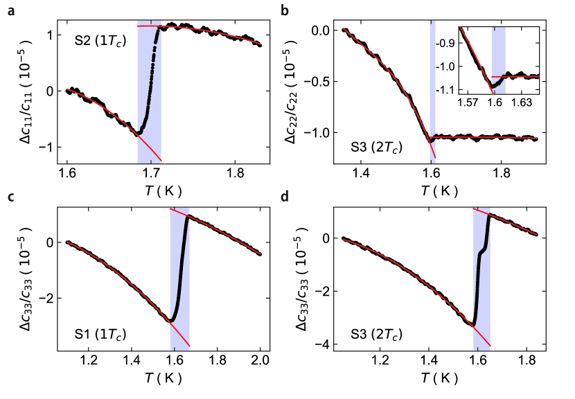
Figure 15: Step Discontinuities in Compressional Moduli. Relative changes in compressional moduli across $T_{c}$ (black points). The magnitude of the step discontinuity in compressional moduli is defined as the difference between polynomial fits to the data above and below $T_{c}$ (red lines). The uncertainty is estimated from the finite temperature range close to $T_{c}$ in which the data deviates significantly from these fits (indicated in blue). Extracted values are given in Table 4. The elastic moduli shown are $c_{11}$ (panel a) and $c_{33}$ (panel c) for samples with one transition and $c_{22}$ (panel b) and $c_{33}$ (panel d) for samples with two transitions. The inset of panel b shows the relative change in $c_{22}$ close to $T_{c}$.

Elastic Modulus	Step in $\frac{\Delta c}{c}$	$\frac{dT_{c}}{d\varepsilon_{ii}}~{}\left(\frac{\mathrm{K}}{\mathrm{\%\,strain}}\right)$	$\frac{dT_{c}}{d\sigma_{ii}}~{}\left(\frac{\mathrm{K}}{\mathrm{GPa}}\right)$	$\frac{dT_{c}}{d\sigma_{ii}}~{}\left(\frac{\mathrm{K}}{\mathrm{GPa}}\right)$ from [25]
$c_{11}$ ($1T_{c}$)	$-(2.2\pm 0.2)\times 10^{-5}$	$-0.23\pm 0.02$	$-0.50\pm 0.03$	-0.87
$c_{22}$ ($2T_{c}$)	$-(0.13\pm 0.07)\times 10^{-5}$	$-0.07\pm 0.02$	$-0.09\pm 0.02$	—
$c_{33}$ ($1T_{c}$)	$-(4.4\pm 0.3)\times 10^{-5}$	$0.34\pm 0.02$	$0.60\pm 0.03$	0.56
$c_{33}$ ($2T_{c}$)	$-(4.7\pm 0.2)\times 10^{-5}$	$0.35\pm 0.02$	$0.62\pm 0.03$	0.56

Table 4: Ehrenfest Analysis. Derivatives of the critical temperature with respect to strain $dT_{c}/d\varepsilon$ are calculated based on the magnitudes of the discontinuities in $\Delta c/c$ extracted according to Figure 15. Values of the absolute elastic moduli and respective uncertainties are taken from Theuss et al. [45] and the size of the specific heat jump (or more precisely $\Delta C/T$) is taken to be $196\pm 18$ mJ/(mol K²) from Figure 14. Knowledge of the signs of $dT_{c}/d\varepsilon$ is required for the correct calculation of $dT_{c}/d\sigma$. Since 13 only yields their absolute value, the signs are chosen according to uniaxial stress experiments [25]. The last column shows a comparison to values from said uniaxial stress experiments in Girod et al. [25].

The derivatives of the critical temperature with respect to stress can be calculated from the derivatives with respect to strain via

$$\begin{pmatrix}dT_{c}/d\sigma_{xx}\\ dT_{c}/d\sigma_{yy}\\ dT_{c}/d\sigma_{zz}\\ \end{pmatrix}=\begin{pmatrix}c11&c12&c13\\ c12&c22&c23\\ c13&c23&c33\\ \end{pmatrix}^{-1}\begin{pmatrix}dT_{c}/d\varepsilon_{xx}\\ dT_{c}/d\varepsilon_{yy}\\ dT_{c}/d\varepsilon_{zz}\\ \end{pmatrix}.$$ (14)

The resulting values are given in Table 4, along with values measured in uniaxial stress experiments [25]. The elastic tensor used for this calculation is again taken from Theuss et al. [45]. Note that the analysis in Equation 14 requires knowledge about the signs of $dT_{c}/d\varepsilon_{ii}$, whereas the Ehrenfest relations in Equation 13 only yield their absolute values. For a correct analysis from our data, signs according to Girod et al. [25] were assumed.

VII.6 UTe₂ Fermi Surface and Superconducting Gap

VII.6.1 Density Functional Theory

Density-functional theory calculations are used to examine the orbital character of the electronic states in the vicinity of the chemical potential. The self-consistent field calculation is performed in the same way as in Theuss et al. [45], by additionally considering the Hubbard $U$ for the uranium $5f$ electrons. The full-potential linearized augmented plane wave method [47] calculations employed the generalized gradient approximation [48] for the exchange correlation, wave function and potential energy cutffs of 16 and 200 Ry, respectively, and muffin-tin sphere radii of $1.35\text{\,}\mathrm{\SIUnitSymbolAngstrom}$. Spin-orbit coupling was fully taken into account in the assumed nonmagnetic state. We set $U=2$ eV to obtain a quasi 2D Fermi surface [30, 31], which qualitatively accounts for the recent experiments. Along the high-symmetry lines in the Brillouin zone ($\Lambda$, $\Sigma$, and $\Delta$ lines, see Figure 16c) and on a dense 50$\times$50$\times$50 $k$-point mesh, the (Kramers degenerate) band energy and wave functions are generated, and the orbital components of each doublet are calculated within the atom-centered spheres of radius $1.35\text{\,}\mathrm{\SIUnitSymbolAngstrom}$. In Figure 16, the orbital components are shown on the Fermi surface (panel a—the visualization of the Fermi surface is done with FermiSurfer [49]) and along the band dispersion (panel b).

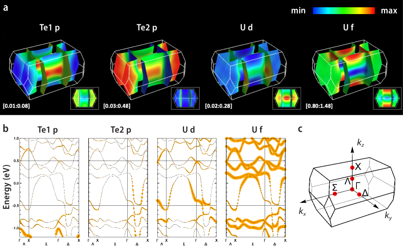
Figure 16: DFT Fermi Surface and Band Structure. (a) Fermi surface of UTe₂ calculated with $U=2$ eV. Fermi surfaces are colored according to their orbital Te1 $p$, Te2 $p$, U $d$, and U $f$ content, from left to right, respectively. Color scales are rescaled between each plot, but respective minimum and maximum values are given to the bottom left of each panel. (b) Band structure calculated with the same parameters as in (a). Orange circles are sized according to the orbital weight of Te1 $p$, Te2 $p$, U $d$, and U $f$ (from left to right) on each individual band. (c) UTe₂ Brillouin zone.

VII.6.2 Tight Binding Model

Figure 16 motivates a tight binding model constructed from two quasi-one-dimensional chain Fermi surfaces: one chain from the Te(2) 5$p$ orbitals, and one from the U 6$d$ orbitals. This model faithfully captures the shape of the Fermi surface measured by quantum oscillations (see [41]). This Fermi surface is quite similar to that calculated for ThTe₂, which has no $f$ electrons—while the $f$ electrons in UTe₂ hybridize strongly with both bands, the predominant effect is to enhance the cyclotron masses and shift the chemical potential, without strongly modifying the Fermi surface shape.

There are two uranium atoms that form a dimer in the center of the conventional unit cell shown in Figure 5a of the main text. The dominant tight binding parameters will be the chemical potential $\mu_{\rm U}$, the intra-dimer overlap $\Delta_{\rm U}$, the hopping $t_{\rm U}$ along the uranium chain in the $a$ direction, the hopping $t^{\prime}_{\rm U}$ to other uranium in the dimer along the chain direction, the hoppings $t_{ch,{\rm U}}$ and $t^{\prime}_{ch,{\rm U}}$ between chains in the $a-b$ plane, and the hopping $t_{z,{\rm U}}$ between chains along the $c$ axis. The two bands from the two uranium sites then come from diagonalizing the following matrix:

$$E_{\rm U}={\tiny\begin{bmatrix}\mu_{\rm U}-2t_{\rm U}\cos k_{x}a-2t_{ch,{\rm U}}\cos k_{y}b&-\Delta_{\rm U}-2t^{\prime}_{\rm U}\cos k_{x}a-2t^{\prime}_{ch,{\rm U}}\cos k_{y}b-4t_{z,{\rm U}}e^{-ik_{z}c/2}\cos k_{x}\frac{a}{2}\cos k_{y}\frac{b}{2}\\ -\Delta_{\rm U}-2t^{\prime}_{\rm U}\cos k_{x}a-2t^{\prime}_{ch,{\rm U}}\cos k_{y}b-4t_{z,{\rm U}}e^{ik_{z}c/2}\cos k_{x}\frac{a}{2}\cos k_{y}\frac{b}{2}&\mu_{\rm U}-2t_{\rm U}\cos k_{x}a-2t_{ch,{\rm U}}\cos k_{y}b\end{bmatrix}}.$$ (15)

There are in principle 4 Te(2) sites per conventional unit cell, but by including only nearest-neighbor hopping in the $a-b$ plane, the problem is again reduced to diagonalizing a $2\times 2$ matrix. The dominant tight binding parameters are then the chemical potential $\mu_{\rm Te}$, the intra-unit-cell overlap $\Delta_{\rm Te}$ between the two Te(2) atoms along the chain direction, the hopping $t_{\rm Te}$ along the Te(2) chain in the $b$ direction, the hopping $t_{ch,{\rm Te}}$ between chains in the $a$ direction, and the hopping $t_{z,{\rm Te}}$ between chains along the $c$ axis. The tight binding matrix is:

$$E_{\rm Te}={\tiny\begin{bmatrix}\mu_{\rm Te}-2t_{ch,{\rm Te}}\cos k_{x}a&-\Delta_{\rm Te}-t_{\rm te}e^{-ik_{y}b}-2t_{z{\rm,Te}}\cos k_{z}\frac{c}{2}\cos k_{x}\frac{a}{2}\cos k_{y}\frac{b}{2}\\ -\Delta_{\rm Te}-t_{\rm te}e^{ik_{y}b}-2t_{z{\rm,Te}}\cos k_{z}\frac{c}{2}\cos k_{x}\frac{a}{2}\cos k_{y}\frac{b}{2}&\mu_{\rm Te}-2t_{ch,{\rm Te}}\cos k_{x}a\end{bmatrix}}.$$ (16)

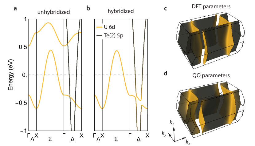
Figure 17: Tight Binding Model. (a-c) Tight binding model with parameters to match DFT results. (a) Unhybridized bands formed by uranium $6d$ (yellow) and tellurium (2) $5p$ (gray) electrons. Bands crossing the Fermi level are hybridized in (b) and the resulting Fermi surface is shown in (c). Colors represent a projection on original U/Te(2) bands. (d) Fermi surface from tight binding model with parameters to match quantum oscillation results [41].

The resultant bands are plotted in Figure 17a. The tight binding parameters were chosen to roughly match the DFT result shown in Figure 16 and are given in Table 5. The two bands crossing the Fermi energy can be hybridized to form the electron and hole pocket. We use an isotropic in momentum hybridization $\delta$ and chose its value to roughly match the DFT result. The resultant two bands that cross the Fermi energy are shown in Figure 17b, and the 3D Fermi surface is shown in Figure 17c. The predominant difference between the FS calculated with $U=2$ eV and the FS reported by Eaton et al. [41] is that the latter was chosen with the opposite-sign dispersion along the $c$-axis. Tight binding parameters chosen to roughly match the FS reported in Eaton et al. [41] are also given in Table 5, with the resultant FS shown in Figure 17d.

	$\Delta_{\rm U}$	$t_{\rm U}$	$t^{\prime}_{\rm U}$	$t_{ch,{\rm U}}$	$t^{\prime}_{ch,{\rm U}}$	$t_{z,{\rm U}}$	$\mu_{\rm Te}$	$\Delta_{\rm Te}$	$t_{\rm Te}$	$t_{ch,{\rm Te}}$	$t_{z,{\rm Te}}$	$\delta$
DFT	0.40	0.15	0.08	0.01	0.00	-0.03	-1.80	-1.50	-1.50	0.00	-0.05	0.09
QO	0.05	0.10	0.08	0.01	0.00	0.04	-1.80	-1.50	-1.50	-0.03	-0.5	0.10

Table 5: All parameters given in eV.

VII.6.3 Superconducting Gap

When considering the symmetries of superconducting gaps, it is necessary to distinguish the cases of weak and strong spin-orbit coupling: UTe₂ likely falls in the latter category. However, since the orthorhombic point group of UTe₂ ($D_{2h}$) is inversion symmetric, one can still label irreducible representations as even or odd. This classification is used to distinguish spin singlet (even) or triplet (odd) superconductors. Since UTe₂ is most likely a spin-triplet superconductor, the possible irreducible representations of the order parameter are $A_{u}$, $B_{1u}$, $B_{2u}$, and $B_{3u}$. In the strong spin-orbit limit, they correspond to the following $\vec{d}$-vectors [50]

$$\vec{d}_{A_{u}} =\left\{\alpha k_{x},\beta k_{y},\gamma k_{z}\right\},$$ (17)

$$\vec{d}_{B_{1u}} =\left\{\alpha k_{y},\beta k_{x},\gamma k_{x}k_{y}k_{z}\right\},$$ (18)

$$\vec{d}_{B_{2u}} =\left\{\alpha k_{z},\beta k_{x}k_{y}k_{z},\gamma k_{x}\right\},$$ (19)

$$\vec{d}_{B_{3u}} =\left\{\alpha k_{x}k_{y}k_{z},\beta k_{z},\gamma k_{y}\right\},$$ (20)

where $\alpha$, $\beta$, and $\gamma$ are real constants and the momentum dependence of the superconducting gap is given by

$$\Delta\left(\vec{k}\right)=\sqrt{\vec{d}\cdot\vec{d}^{\star}\pm\left|\vec{d}\times\vec{d}^{\star}\right|}.$$ (21)

Here, $\vec{d}^{\star}$ is the complex conjugate of $\vec{d}$. The $A_{u}$ order parameter is fully gapped, whereas the $B_{1u}$, $B_{2u}$, and $B_{3u}$ order parameters have point nodes along the $k_{z}$, $k_{y}$, and $k_{x}$ directions respectively. A $B_{1u}$ gap is thus also fully gapped on the Fermi surface of UTe₂ found by quantum oscillations [42, 41] and only exhibits point nodes on a putative Fermi pocket enclosing the $\Gamma$-point [51].

The gap structures shown in the main text are calculated at $k_{z}=0$ with $\alpha=\beta=\gamma$. A slight anisotropy in these parameters can change the exact shape of the momentum dependence of the different gap symmetries, but will not change their nodal structure.

References

- Tsuei and Kirtley [2000] C. C. Tsuei and J. R. Kirtley, Pairing symmetry in cuprate superconductors, Reviews of Modern Physics 72, 969 (2000).
- Ghosh et al. [2021] S. Ghosh, A. Shekhter, F. Jerzembeck, N. Kikugawa, D. A. Sokolov, M. Brando, A. P. Mackenzie, C. W. Hicks, and B. J. Ramshaw, Thermodynamic evidence for a two-component superconducting order parameter in Sr2RuO4, Nature Physics 17, 199 (2021).
- Rice and Sigrist [1995] T. M. Rice and M. Sigrist, Sr2RuO4: an electronic analogue of 3He?, Journal of Physics: Condensed Matter 7, L643 (1995).
- Mackenzie et al. [2017] A. P. Mackenzie, T. Scaffidi, C. W. Hicks, and Y. Maeno, Even odder after twenty-three years: the superconducting order parameter puzzle of Sr2RuO4, npj Quantum Materials 2, 40 (2017).
- Sato and Ando [2017] M. Sato and Y. Ando, Topological superconductors: a review, Rep. Prog. Phys. 80, 076501 (2017).
- Metz et al. [2019] T. Metz, S. Bae, S. Ran, I.-L. Liu, Y. S. Eo, W. T. Fuhrman, D. F. Agterberg, S. M. Anlage, N. P. Butch, and J. Paglione, Point-node gap structure of the spin-triplet superconductor UTe2, Physical Review B 100, 220504 (2019).
- Ran et al. [2019a] S. Ran, C. Eckberg, Q.-P. Ding, Y. Furukawa, T. Metz, S. R. Saha, I.-L. Liu, M. Zic, H. Kim, J. Paglione, and N. P. Butch, Nearly ferromagnetic spin-triplet superconductivity, Science 365, 684 (2019a).
- Ishihara et al. [2023] K. Ishihara, M. Roppongi, M. Kobayashi, K. Imamura, Y. Mizukami, H. Sakai, P. Opletal, Y. Tokiwa, Y. Haga, K. Hashimoto, and T. Shibauchi, Chiral superconductivity in UTe2 probed by anisotropic low-energy excitations, Nature Communications 14, 2966 (2023).
- Kittaka et al. [2020] S. Kittaka, Y. Shimizu, T. Sakakibara, A. Nakamura, D. Li, Y. Homma, F. Honda, D. Aoki, and K. Machida, Orientation of point nodes and nonunitary triplet pairing tuned by the easy-axis magnetization in UTe2, Physical Review Research 2, 032014 (2020).
- Aoki et al. [2019] D. Aoki, A. Nakamura, F. Honda, D. Li, Y. Homma, Y. Shimizu, Y. J. Sato, G. Knebel, J.-P. Brison, A. Pourret, D. Braithwaite, G. Lapertot, Q. Niu, M. Vališka, H. Harima, and J. Flouquet, Unconventional Superconductivity in Heavy Fermion UTe2, Journal of the Physical Society of Japan 88, 043702 (2019).
- Ran et al. [2019b] S. Ran, I.-L. Liu, Y. S. Eo, D. J. Campbell, P. M. Neves, W. T. Fuhrman, S. R. Saha, C. Eckberg, H. Kim, D. Graf, F. Balakirev, J. Singleton, J. Paglione, and N. P. Butch, Extreme magnetic field-boosted superconductivity, Nature Physics 15, 1250 (2019b).
- Hayes et al. [2021] I. M. Hayes, D. S. Wei, T. Metz, J. Zhang, Y. S. Eo, S. Ran, S. R. Saha, J. Collini, N. P. Butch, D. F. Agterberg, A. Kapitulnik, and J. Paglione, Multicomponent superconducting order parameter in UTe2, Science 373, 797 (2021).
- Wei et al. [2022] D. S. Wei, D. Saykin, O. Y. Miller, S. Ran, S. R. Saha, D. F. Agterberg, J. Schmalian, N. P. Butch, J. Paglione, and A. Kapitulnik, Interplay between magnetism and superconductivity in UTe2, Physical Review B 105, 024521 (2022).
- Jiao et al. [2020] L. Jiao, S. Howard, S. Ran, Z. Wang, J. O. Rodriguez, M. Sigrist, Z. Wang, N. P. Butch, and V. Madhavan, Chiral superconductivity in heavy-fermion metal UTe2, Nature 579, 523 (2020).
- Bae et al. [2021] S. Bae, H. Kim, Y. S. Eo, S. Ran, I.-l. Liu, W. T. Fuhrman, J. Paglione, N. P. Butch, and S. M. Anlage, Anomalous normal fluid response in a chiral superconductor UTe2, Nature Communications 12, 2644 (2021).
- Rosa et al. [2022] P. F. S. Rosa, A. Weiland, S. S. Fender, B. L. Scott, F. Ronning, J. D. Thompson, E. D. Bauer, and S. M. Thomas, Single thermodynamic transition at 2 K in superconducting UTe2 single crystals, Communications Materials 3, 1 (2022).
- Thomas et al. [2021] S. M. Thomas, C. Stevens, F. B. Santos, S. S. Fender, E. D. Bauer, F. Ronning, J. D. Thompson, A. Huxley, and P. F. S. Rosa, Spatially inhomogeneous superconductivity in UTe2, Physical Review B 104, 224501 (2021).
- Aoki et al. [2020] D. Aoki, F. Honda, G. Knebel, D. Braithwaite, A. Nakamura, D. X. Li, Y. Homma, Y. Shimizu, Y. J. Sato, J. P. Brison, and J. Flouquet, Multiple superconducting phases and unusual enhancement of the upper critical field in UTe2, Journal of the Physical Society of Japan 89, 053705 (2020).
- Braithwaite et al. [2019] D. Braithwaite, M. Vališka, G. Knebel, G. Lapertot, J.-P. Brison, A. Pourret, M. E. Zhitomirsky, J. Flouquet, F. Honda, and D. Aoki, Multiple superconducting phases in a nearly ferromagnetic system, Communications Physics 2, 147 (2019).
- Matsumura et al. [2023] H. Matsumura, H. Fujibayashi, K. Kinjo, S. Kitagawa, K. Ishida, Y. Tokunaga, H. Sakai, S. Kambe, A. Nakamura, Y. Shimizu, Y. Homma, D. Li, F. Honda, and D. Aoki, Large reduction in the a-axis Knight shift on UTe2 with K, Journal of the Physical Society of Japan 92, 063701 (2023).
- Iguchi et al. [2023] Y. Iguchi, H. Man, S. M. Thomas, F. Ronning, P. F. S. Rosa, and K. A. Moler, Microscopic imaging homogeneous and single phase superfluid density in UTe2, Physical Review Letters 130, 196003 (2023).
- Xu et al. [2019] Y. Xu, Y. Sheng, and Y.-f. Yang, Quasi-two-dimensional fermi surfaces and unitary spin-triplet pairing in the heavy fermion superconductor UTe2, Physical Review Letters 123, 217002 (2019).
- Fujibayashi et al. [2022] H. Fujibayashi, G. Nakamine, K. Kinjo, S. Kitagawa, K. Ishida, Y. Tokunaga, H. Sakai, S. Kambe, A. Nakamura, Y. Shimizu, Y. Homma, D. Li, F. Honda, and D. Aoki, Superconducting order parameter in UTe2 determined by knight shift measurement, Journal of the Physical Society of Japan 91, 043705 (2022).
- Nakamine et al. [2021a] G. Nakamine, K. Kinjo, S. Kitagawa, K. Ishida, Y. Tokunaga, H. Sakai, S. Kambe, A. Nakamura, Y. Shimizu, Y. Homma, D. Li, F. Honda, and D. Aoki, Anisotropic response of spin susceptibility in the superconducting state of UTe2 probed with 125Te-NMR measurement, Physical Review B 103, L100503 (2021a).
- Girod et al. [2022] C. Girod, C. R. Stevens, A. Huxley, E. D. Bauer, F. B. Santos, J. D. Thompson, R. M. Fernandes, J.-X. Zhu, F. Ronning, P. F. S. Rosa, and S. M. Thomas, Thermodynamic and electrical transport properties of UTe2 under uniaxial stress, Physical Review B 106, L121101 (2022).
- Nakamine et al. [2021b] G. Nakamine, K. Kinjo, S. Kitagawa, K. Ishida, Y. Tokunaga, H. Sakai, S. Kambe, A. Nakamura, Y. Shimizu, Y. Homma, D. Li, F. Honda, and D. Aoki, Inhomogeneous superconducting state probed by 125Te NMR on UTe2, Journal of the Physical Society of Japan 90, 064709 (2021b).
- Machida [2020] K. Machida, Theory of spin-polarized superconductors —an analogue of superfluid 3He A-phase, Journal of the Physical Society of Japan 89, 033702 (2020).
- Machida [2021] K. Machida, Nonunitary triplet superconductivity tuned by field-controlled magnetization: URhGe, UCoGe, and UTe2, Physical Review B 104, 014514 (2021).
- Nevidomskyy [2020] A. H. Nevidomskyy, Stability of a nonunitary triplet pairing on the border of magnetism in UTe2 (2020), arXiv:2001.02699 [cond-mat.supr-con] .
- Ishizuka et al. [2019] J. Ishizuka, S. Sumita, A. Daido, and Y. Yanase, Insulator-metal transition and topological superconductivity in UTe2 from a first-principles calculation, Physical Review Letters 123, 217001 (2019).
- Shishidou et al. [2021] T. Shishidou, H. G. Suh, P. M. R. Brydon, M. Weinert, and D. F. Agterberg, Topological band and superconductivity in UTe2, Physical Review B 103, 104504 (2021).
- Choi et al. [2023] H. C. Choi, S. H. Lee, and B.-J. Yang, Correlated normal state fermiology and topological superconductivity in UTe2 (2023), arXiv:2206.04876 [cond-mat.supr-con] .
- Shaffer and Chichinadze [2022] D. Shaffer and D. V. Chichinadze, Chiral superconductivity in UTe2 via emergent symmetry and spin-orbit coupling, Physical Review B 106, 014502 (2022).
- Hazra and Volkov [2022] T. Hazra and P. Volkov, Pair-kondo effect: a mechanism for time-reversal broken superconductivity and finite-momentum pairing in UTe2 (2022), arXiv:2210.16293 [cond-mat.supr-con] .
- Chang et al. [2023] Y.-Y. Chang, K. V. Nguyen, K.-L. Chen, Y.-W. Lu, C.-Y. Mou, and C.-H. Chung, Topological Kondo superconductors (2023), arXiv:2301.00538 [cond-mat.str-el] .
- Ushida et al. [2023] K. Ushida, T. Yanagisawa, R. Hibino, M. Matsuda, H. Hidaka, H. Amitsuka, G. Knebel, J. Flouquet, and D. Aoki, Lattice instability of UTe2 studied by ultrasonic measurements, JPS Conference Proceedings 38, 011021 (2023).
- Rehwald [1973] W. Rehwald, The study of structural phase transitions by means of ultrasonic experiments, Advances in Physics 22, 721 (1973).
- Note [1] The fully symmetrized coupling is .
- Note [5] It is possible to come up with mixed-parity order parameters that do not have jumps in shear elastic moduli, e.g. . Roughly speaking, these mixed-parity order parameters do not produce jumps in shear moduli because the product of an even-parity and an odd-parity object is itself an odd-parity object. Strains, on the other hand, are always even-parity objects. Thus, a term that is one power of an even-parity order parameter, one power of an odd-parity order parameter, and one power of strain, is an odd-parity term. Such terms are forbidden, as the free energy is even parity. These scenarios have no experimental backing, but have been proposed on theoretical grounds [52].
- Sundar et al. [2023] S. Sundar, N. Azari, M. R. Goeks, S. Gheidi, M. Abedi, M. Yakovlev, S. R. Dunsiger, J. M. Wilkinson, S. J. Blundell, T. E. Metz, I. M. Hayes, S. R. Saha, S. Lee, A. J. Woods, R. Movshovich, S. M. Thomas, N. P. Butch, P. F. S. Rosa, J. Paglione, and J. E. Sonier, Ubiquitous spin freezing in the superconducting state of UTe2, Communications Physics 6, 24 (2023).
- Eaton et al. [2023] A. G. Eaton, T. I. Weinberger, N. J. M. Popiel, Z. Wu, A. J. Hickey, A. Cabala, J. Pospisil, J. Prokleska, T. Haidamak, G. Bastien, P. Opletal, H. Sakai, Y. Haga, R. Nowell, S. M. Benjamin, V. Sechovsky, G. G. Lonzarich, F. M. Grosche, and M. Valiska, Quasi-2D Fermi surface in the anomalous superconductor UTe2 (2023), arXiv:2302.04758 [cond-mat.supr-con] .
- Aoki et al. [2022] D. Aoki, H. Sakai, P. Opletal, Y. Tokiwa, J. Ishizuka, Y. Yanase, H. Harima, A. Nakamura, D. Li, Y. Homma, Y. Shimizu, G. Knebel, J. Flouquet, and Y. Haga, First observation of the de Haas–van Alphen Effect and Fermi surfaces in the unconventional superconductor UTe2, Journal of the Physical Society of Japan 91, 083704 (2022).
- Broyles et al. [2023] C. Broyles, Z. Rehfuss, H. Siddiquee, J. A. Zhu, K. Zheng, M. Nikolo, D. Graf, J. Singleton, and S. Ran, Revealing a 3D Fermi surface pocket and electron-hole tunneling in UTe2 with quantum oscillations, Phys. Rev. Lett. 131, 036501 (2023).
- Ran et al. [2021] S. Ran, I.-L. Liu, S. R. Saha, P. Saraf, J. Paglione, and N. P. Butch, Comparison of Two Different Synthesis Methods of Single Crystals of Superconducting Uranium Ditelluride, JoVE (Journal of Visualized Experiments) , e62563 (2021).
- Theuss et al. [2023] F. Theuss, G. de la Fuente Simarro, A. Shragai, G. Grissonnanche, I. M. Hayes, S. Saha, T. Shishidou, T. Chen, S. Nakatsuji, S. Ran, M. Weinert, N. P. Butch, J. Paglione, and B. J. Ramshaw, Resonant ultrasound spectroscopy for irregularly-shaped samples and its application to uranium ditelluride (2023), arXiv:2303.03473 [cond-mat.str-el] .
- Ramshaw et al. [2015] B. J. Ramshaw, A. Shekhter, R. D. McDonald, J. B. Betts, J. N. Mitchell, P. H. Tobash, C. H. Mielke, E. D. Bauer, and A. Migliori, Avoided valence transition in a plutonium superconductor, Proceedings of the National Academy of Sciences of the United States of America 112, 3285 (2015).
- Weinert et al. [2009] M. Weinert, G. Schneider, R. Podloucky, and J. Redinger, FLAPW: Applications and implementations, Journal of Physics: Condensed Matter 21, 084201 (2009).
- Perdew et al. [1996] J. P. Perdew, K. Burke, and M. Ernzerhof, Generalized Gradient Approximation Made Simple, Phys. Rev. Lett. 77, 3865 (1996).
- Kawamura [2019] M. Kawamura, Fermisurfer: Fermi-surface viewer providing multiple representation schemes, Computer Physics Communications 239, 197 (2019).
- Annett [1990] J. F. Annett, Symmetry of the order parameter for high-temperature superconductivity, Advances in Physics 39, 83 (1990).
- Miao et al. [2020] L. Miao, S. Liu, Y. Xu, E. C. Kotta, C.-J. Kang, S. Ran, J. Paglione, G. Kotliar, N. P. Butch, J. D. Denlinger, and L. A. Wray, Low Energy Band Structure and Symmetries of UTe 2 from Angle-Resolved Photoemission Spectroscopy, Physical Review Letters 124, 10.1103/PhysRevLett.124.076401 (2020).
- Ishizuka and Yanase [2021] J. Ishizuka and Y. Yanase, Periodic Anderson model for magnetism and superconductivity in UTe2, Phys. Rev. B 103, 094504 (2021).