Gravitational waves effects in a Lorentz–violating scenario

Abstract

This paper focuses on how the production and polarization of gravitational waves are affected by spontaneous Lorentz symmetry breaking, which is driven by a self–interacting vector field. Specifically, we examine the impact of a smooth quadratic potential and a non–minimal coupling, discussing the constraints and causality features of the linearized Einstein equation. To analyze the polarization states of a plane wave, we consider a fixed vacuum expectation value (VEV) of the vector field. Remarkably, we verify that a space–like background vector field modifies the polarization plane and introduces a longitudinal degree of freedom. In order to investigate the Lorentz violation effect on the quadrupole formula, we use the modified Green function. Finally, we show that the space–like component of the background field leads to a third–order time derivative of the quadrupole moment, and the bounds for the Lorentz–breaking coefficients are estimated as well.

I Introduction

Understanding the spacetime structure at the Planck scale and developing a corresponding quantum theory of gravity is one of the most challenging open questions in modern physics. At such high–energy scales, it is possible that some of the low–energy symmetries present in the standard model of particles and gravity, such as Lorentz and CPT symmetries, may be violated. This phenomenon has been observed in various theories, including some string theory vacuum 1 ; 1.2 , Loop Quantum Gravity 2 ; 2.1 , non–commutative geometry (3, ; araujo2023thermodynamics, ; heidari2023gravitational, ), Horava Gravity (4, ), and Very Special Relativity (5, ; furtado2023thermal, ).

The Standard Model Extension (SME) 6 ; 6.1 provides a general framework for probing the remnants of Lorentz–violating effects at low–energy regimes. By considering coupling terms between the Standard Model fields and Lorentz–violating coefficients, several studies have been addressed in a different context, such as photons (7, ; araujo2021thermodynamic, ; araujo2021higher, ; araujo2022particles, ; araujo2021bouncing, ; araujo2022thermal, ), neutrinos (8, ), muons (9, ), quantum rings ww1 , and hydrogen atoms (10, ), among others filho2022thermodynamics ; li2017application ; cambiaso2012massive ; ww2 ; ww3 ; ww4 . A comprehensive list of tests for Lorentz and CPT symmetry breaking can be found in Ref. (11, ). In addition, in order to incorporate gravity into the Standard Model Extension (SME), we must assume the possibility of spontaneous Lorentz symmetry violation. This is typically achieved by introducing self–interacting tensor fields with a non–null vacuum bluhm2008spontaneous .

Gravitational wave detection was one of the most important events for high–energy physics. Two notable events took place in 2015 and were announced on February 11th, 2016 by the VIRGO and LIGO laboratories. The first event, GW150914, was detected on September 14th, 2015 12 . The second one, GW151226, was detected on December 26th, 2015. Both events were caused by the coalescence of two black holes located at distances of approximately 410 Mpc and 440 Mpc, respectively 13 . The detection of gravitational waves from these events represents a major milestone in the study of black holes and the nature of gravity, opening up new avenues for research and providing important insights into the workings of the universe at the most fundamental level aa2023analysis .

One relatively simple field that breaks the Lorentz symmetry is the bumblebee field $B_{\mu}$. The Lorentz symmetry is spontaneously broken by the dynamics of $B_{\mu}$, which acquires a non–zero vacuum expectation value (VEV) 15 ; 16 ; maluf2019antisymmetric . This model was originally considered in the context of string theory, where LSB is triggered by the potential $V(B^{\mu})=\lambda(B^{\mu}B_{\mu}\mp b^{2})^{2}/2$.

This work focuses on analyzing the modifications in the polarization and production of gravitational waves due to Lorentz symmetry breaking (LSB) in the weak field regime. In particular, we investigate the effects of the spontaneous breaking of Lorentz symmetry, triggered by the bumblebee vector field. Then, we solve the modified wave equation for the perturbation field and compare the polarization tensor of the modified gravitational wave solution with the conventional case. Next we introduce a current $J_{\mu\nu}$ to the model and derive a Green function for the timelike $b^{\mu}=(b^{0},0)$ and spacelike $b^{\mu}=(0,{\bf b})$ configurations for the bumblebee VEV. Subsequently, we obtain a modified quadrupole formula for the graviton, which enables us to compare the perturbation for the modified equation with the usual one and to identify the modifications in the theory.

II Modifying the Graviton Wave Equation

The minimal extension of the gravity theory, including the Lorentz–violating terms is given by the following expression 17

$$S=S_{EH}+S_{LV}+S_{matter}.$$ (1)

The first term refers to the usual Einstein–Hilbert action,

$$S_{EH}=\int d^{4}x\;\sqrt{-g}\frac{2}{\kappa^{2}}(R-2\Lambda),$$ (2)

where $R$ is the curvature scalar and $\Lambda$ is the cosmological constant, which will not be considered in this analysis. The $S_{LV}$ term consists of the coupling between the bumblebee field and the curvature of spacetime

$$S_{LV}=\int d^{4}x\;\sqrt{-g}\frac{2}{\kappa^{2}}(uR+s^{\mu\nu}R_{\mu\nu}+t^{\alpha\beta\mu\nu}R_{\alpha\beta\mu\nu}),$$ (3)

where $u$, $s^{\mu\nu}$ and $t^{\alpha\beta\mu\nu}$ are dynamical fields with zero mass dimension nascimento2022vacuum . And the last term represents the matter–gravity couplings which, in principle, should include all fields of the standard model as well as the possible interactions with the coefficients $u$, $s^{\mu\nu}$ and $t^{\alpha\beta\mu\nu}$.

The dynamics of the bumblebee field $B^{\mu}$ is dictated by the action 18 ; hassanabadi2023gravitational

$$S_{B}=\int d^{4}x\;\sqrt{-g}\left[-\frac{1}{4}B^{\mu\nu}B_{\mu\nu}+\frac{2\xi}{\kappa^{2}}B^{\mu}B^{\nu}R_{\mu\nu}-V(B^{\mu}B_{\mu}\mp b^{2})\right],$$ (4)

where we introduced the field strength $B_{\mu\nu}=\partial_{\mu}B_{\nu}-\partial_{\nu}B_{\mu}$ in analogy with the electromagnetic field tensor $F_{\mu\nu}$. In fact, the bumblebee models are not only used as toy models to investigate the excitation originating from the LSB mechanism. They also provide an alternative to $U(1)$ gauge theory for photons 19 . In this theory, they appear as Nambu–Goldstone modes due to spontaneous Lorentz violation 20 , rather than fundamental particles.

The gravity–bumblebee coupling can be represented by Eq. (3) defining

$$u=\frac{1}{4}\xi B^{\alpha}B_{\alpha},\quad s^{\mu\nu}=\xi\left(B^{\mu}B^{\nu}-\frac{1}{4}g^{\mu\nu}B^{\alpha}B_{\alpha}\right),\quad t^{\alpha\beta\mu\nu}=0,$$ (5)

and the potential $V(X)$ reads

$$V=\frac{\lambda}{2}\left(B^{\mu}B_{\mu}\mp b^{2}\right)^{2}.$$ (6)

It is responsible for triggering spontaneously the Lorentz violation and breakdown of the diffeomorphism. Here, $b^{2}$ is a positive constant that stands for the non–zero vacuum expectation value of this field. In our study, we aim to investigate how the coupling between gravity and the bumblebee field affects the behavior of graviton. To do so, we consider the linearized version of the metric $g_{\mu\nu}$ with the Minkowski background and the bumblebee field $B_{\mu}$, which is split into the vacuum expectation values $b_{\mu}$ and the quantum fluctuations $\tilde{B}^{\mu}$

$$g_{\mu\nu} = \eta_{\mu\nu}+\kappa h_{\mu\nu},$$

$$B_{\mu} = b_{\mu}+\tilde{B}_{\mu},$$

$$B^{\mu} = b^{\mu}+\tilde{B}^{\mu}-\kappa b_{\nu}h^{\mu\nu}.$$ (7)

By multiplying the linearized equation of motion with $p^{\mu}p^{\nu}$, $b^{\mu}b^{\nu}$, $p^{(\mu}b^{\nu)}$, the set of constraints are obtained

$$p_{\mu}p_{\nu}h^{\mu\nu}=0,\quad b_{\mu}b_{\nu}h^{\mu\nu}=0,\quad p_{(\mu}b_{\nu)}h^{\mu\nu}=0,\quad h=0,\quad p_{\mu}h^{\mu}_{\nu}=0,\quad b_{\mu}h^{\mu}_{\nu}=0.$$ (8)

Despite the violation of the diffeomorphism symmetry, twelve constraints in Eq. (8) enables only two propagating degrees of freedom, as for the usual Lorentz–invariant graviton. In other words, no graviton mass is produced due to the interaction with the bumblebee field at leading order. The modified dispersion relation (MDR) associated with the physical pole is given by 22

$$[p^{2}+\xi(b\cdot p)^{2}]h_{\mu\nu}=0,$$ (9)

where $b\cdot p=\eta_{\mu\nu}b^{\mu}p^{\mu}$, with $p^{\mu}=(p^{0},{\mathbf{p}})$ and $b^{\mu}=(b^{0},{\mathbf{b}})$. It turns out that the MDR preserves both stability and causality 22 . Also, the respective thermodynamic behavior based on such a modified dispersion relation was addressed in the literature recently by Araújo Filho filho2021thermal .

III Polarization states

Studying the polarization of gravitational waves is crucial to gaining insights into the properties of the source and the nature of spacetime. It provides unique information about the motion of massive objects and can reveal any effects encountered during their journey, making it a critical area of research in modern astrophysics le2017theory ; liang2017polarizations ; zhang2018velocity ; hou2018polarizations ; mewes2019signals ; liang2022polarizations . In this sense, we obtain the modified polarization tensor to the free perturbation, satisfying the constraints (8) and the dispersion relation (9). The source–free equation has the form

$$[\Box+\xi(b\cdot\partial)^{2}]h_{\mu\nu}(x)=0.$$ (10)

Consider a plane–wave $h_{\mu\nu}=\varepsilon_{\mu\nu}e^{i(\omega t-kz)}$ propagating along the $z$ axis with momentum $p^{\mu}=(p^{0},0,0,p^{3})$. The constraint $b_{\mu}h^{\mu}_{\nu}=0$ forbids any state in the direction of the background vector $b^{\mu}$.

For a timelike $b^{\mu}=(b^{0},0,0,0)$, the polarization tensor reads

$$\varepsilon_{\mu\nu}=\left(\begin{array}[]{cccc}0&0&0&0\\ 0&\varepsilon_{11}&\varepsilon_{12}&0\\ 0&\varepsilon_{12}&-\varepsilon_{11}&0\\ 0&0&0&0\end{array}\right),$$ (11)

preserving two Lorentz invariant transversal modes. Nevertheless, the group velocity is modified by

$$p^{0}=\frac{p_{3}}{\sqrt{1+(b^{0})^{2}\xi}}.$$ (12)

Now let us consider a spacelike vector with a spatial component along $b^{\mu}=(0,0,0,b^{3})$. The polarization tensor still has the form of Eq. (11), albeit the wave propagates with dispersion relation

$$p^{0}=p^{3}\sqrt{1-\xi(b^{0})^{2}}.$$ (13)

Similar modified dispersion relations were obtained for gauge–invariant containing higher mass dimension operators (26, ; 27, ). The group velocity $v_{g}=\frac{\partial p^{0}}{\partial p^{3}}=\sqrt{1-\xi(b^{0})^{2}}<1$. Therefore, for a timelike or a spacelike $b^{\mu}$, i.e., with $\vec{b}$ parallel to $\vec{p}$, the transversal characteristic of the gravitational waves is preserved and the wave velocity is slowed by the Lorentz violation.

On the other hand, considering $\vec{b}$ perpendicular to $\vec{p}$, e.g., $b^{\mu}=(0,0,b^{2},0)$, we obtain

$$\varepsilon_{\mu\nu}=\left[\begin{array}[]{cccc}-\frac{1}{2}\varepsilon_{11}&-\varepsilon_{13}&0&\frac{1}{2}\varepsilon_{11}\\ -\varepsilon_{13}&\varepsilon_{11}&0&\varepsilon_{13}\\ 0&0&0&0\\ \frac{1}{2}\varepsilon_{11}&\varepsilon_{13}&0&-\frac{1}{2}\varepsilon_{11}\end{array}\right].$$ (14)

It is worth mentioning that the polarization tensor (14) has two independent states, $\varepsilon_{11}$ and $\varepsilon_{13}$. The plus state $\varepsilon_{11}$ corresponds to the transversal polarization in the $x$ direction and it is present in the Lorentz invariant wave. Nonetheless, the presence of the cross–state $\varepsilon_{13}$ leads to a longitudinal polarization along the $z$ direction – a feature forbidden in the Lorentz invariant theory. In other words, the background vector transforms one transversal into a longitudinal degree of freedom. The dispersion relation, in its turn, is kept invariant

$$p^{0}=p^{3}.$$ (15)

Moreover, the line element is modified by

$$ds^{2} = \left(1-\frac{1}{2}\varepsilon_{11}\right)dt^{2}-(1-\varepsilon_{11})dx^{2}-dy^{2}-\left(1+\frac{1}{2}\varepsilon_{11}\right)dz^{2}+2\varepsilon_{13}dx\otimes dz$$ (16)

$$- 2\varepsilon_{13}dt\otimes dx+\varepsilon_{11}dt\otimes dz.$$

In this manner, the Lorentz–violating gravitational waves produce contractions and dilatations in the $xz$ plane, and also time deformations.

The effects of these modified gravitational waves on particles can be observed by considering the geodesic deviation equation, which for slowly test particle $U^{\mu}\approx(1,0,0,0)$ reads

$$\frac{D^{2}S^{\mu}}{d\tau^{2}}=R^{\mu}_{00\sigma}S^{\sigma},$$ (17)

where the $S^{\mu}$ is the displacement vector. From Eq.(14), the temporal and $y$ components vanish $\frac{D^{2}S^{0}}{d\tau^{2}}=\frac{D^{2}S^{2}}{d\tau^{2}}=0$. Although $h_{00}$ is not zero, no time tilde forces arise in this context. In the $x$ direction, Eq.(17) gives

$$\frac{D^{2}S^{1}}{d\tau^{2}}=\frac{\omega^{2}}{2}\Big{\{}\left(\frac{1}{2}S^{0}-S^{1}\right)h^{1}_{1}+\left(S^{0}-2S^{1}\right)h^{1}_{3}\Big{\}},$$ (18)

whereas the tidal force in the longitudinal direction has the form

$$\frac{D^{2}S^{3}}{d\tau^{2}}=-\frac{\omega^{2}}{2}h^{3}_{1}S^{1}.$$ (19)

For two test particles close enough, their events can be considered simultaneous and the corresponding timelike component $S^{0}$ can be neglected. Note that both plus and cross polarizations contribute to the geodesic deviation in the $x$ direction, while the cross state produces variation along the longitudinal direction only.

IV Gravitational waves production in the presence of the bumblebee field

For the analysis of the production of GW, we add a current $J_{\mu\nu}$ to the homogeneous equation to the graviton field in Eq. (10) resulting in

$$[\Box+\xi(b\cdot\partial)^{2}]h_{\mu\nu}(x)=J_{\mu\nu}(x).$$ (20)

The perturbation is determined by

$$h_{\mu\nu}(x)=\int d^{4}y\;G(x-y)J_{\mu\nu}(y).$$ (21)

For the modified graviton equation, we can represent the Green function in the momentum space

$$\tilde{G}(p)=\frac{1}{p^{2}+\xi(b\cdot p)^{2}},$$ (22)

so that to get $G$ in the configuration space, we may use the inverse Fourier transform. The inversion is made for two particular cases; the first is considering that $b^{\mu}$ has a timelike configuration $b^{\mu}=\left(b^{0},0\right)$, in this case, the Green function resumes to

$$\tilde{G}(p)=\frac{1}{[1+\xi b_{0}^{2}]p_{0}^{2}-\left|{\bf p}\right|},$$ (23)

and the inversion results to

$$G(x-y)=\frac{1}{4\pi\sqrt{1+\xi b_{0}^{2}}r}\delta\left[r-\frac{\tau}{\sqrt{1+\xi b_{0}^{2}}}\right].$$ (24)

The second case is a spacelike configuration $b^{\mu}=(0,{\bf b})$, which will reduce $\tilde{G}(p)$ to

$$\tilde{G}(p)=\frac{1}{p_{0}^{2}-(1-\xi|{\bf b}|^{2}\cos^{2}{\Psi})|{\bf p}|},$$ (25)

where $\Psi$ is the angle between ${\bf p}$ and ${\bf b}$, therefore $\cos^{2}{\Psi}=\cos(\theta)\cos(\theta_{b})+\sin(\theta)\sin(\theta_{b})\cos(\phi_{b}-\phi)$, with ($\theta$, $\phi$) and ($\theta_{b}$, $\phi_{b}$) the angular coordinates of the trivectors ${\bf p}$ and ${\bf b}$, respectively.

The inverse Fourier transform of Eq. (25) expanded to the second order of $|{\bf b}|$ is

$$G(x-y)=G_{R}(x-y)-G_{2}(x-y),$$ (26)

with the second term being given by

$$\begin{split}G_{2}(x-y)=&\frac{\xi}{8\pi r^{3}}\Theta(\tau)\times\\ &\times\left\{(b\cdot r)^{2}\left[\left(\frac{\tau}{r}-1\right)\delta(\tau-r)+\tau\delta^{\prime}(\tau-r)\right]+\tau rb^{2}\cos({2\theta_{b}})\;\delta(\tau-r)\right\}.\end{split}$$ (27)

For the usual Einstein–Hilbert linearized theory, we have the formula for the perturbation

$$h_{ij}(t,{\bf r})=\frac{2G}{r}\frac{d^{2}I_{ij}}{dt^{2}}(t_{r}),$$ (28)

where $t_{r}=t-r$ is the retarded time and $I_{ij}$ is the quadrupole momentum defined as

$$I_{ij}(t)=\int y^{i}y^{j}T^{00}d^{3}y.$$ (29)

With $b^{\mu}=(b^{0},0)$ and considering that $J_{\mu\nu}=16\pi GT_{\mu\nu}$, the perturbations are written as

$$h_{ij}(t,{\bf r})=\frac{2G}{r}\frac{d^{2}I_{ij}}{dt^{2}}(t^{\prime}_{r}),$$ (30)

where the retarded time is modified to $t^{\prime}_{r}=t-r\sqrt{1+b_{0}^{2}}$, evidencing that the waves propagates slower. When $b^{\mu}=(0,{\bf b})$ the perturbation is

$$h_{ij}(t,{\bf r})=\frac{2G}{r}\left[\left(1-\frac{\xi b^{2}}{2}\cos{2\theta_{b}}\right)\frac{d^{2}I_{ij}}{dt^{2}}(t_{r})+\frac{\xi({\bf b}\cdot{\bf r})^{2}}{2r}\frac{d^{3}I_{ij}}{dt^{3}}(t_{r})\right].$$ (31)

Here, we can see the anisotropy in above solution. Such a feature is well–known within the context of theories modified by the bumblebee vector. The vector ${\bf b}$ selects a preferential direction for the wave propagation. Another peculiarity is that a term involving third derivative of the $I_{ij}$ gives rise to. In addition, terms of dipole are still prohibited due to the momentum conservation.

Now, let us analyze the modifications in the simple binary black hole problem pictured in the Fig. 1. It represents the movement of a binary system constituted of two masses $m_{1}$ and $m_{2}$ in the $xy$ plane. The distances from the center of the reference frame to the respective masses are $r_{1}$ and $r_{2}$.

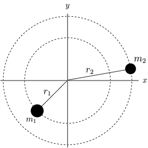
Figure 1: The representation of binary black hole problem.

Furthermore, the density of energy $T^{00}$ is determined from the formula

$$T_{00}=\delta(z)[m_{1}\delta(x-x_{1})\delta(y-y_{1})+m_{2}\delta(x-x_{2})\delta(y-y_{2})],$$ (32)

and the equations of motion of the two particles are

$$x_{1}=\frac{m_{2}l_{0}}{M}\cos{\omega t}, \qquad y_{1}=\frac{m_{2}l_{0}}{M}\sin{\omega t},$$

$$x_{2}=-\frac{m_{1}l_{0}}{M}\cos{\omega t}, \qquad y_{2}=-\frac{m_{1}l_{0}}{M}\sin{\omega t}.$$ (33)

with $M=m_{1}+m_{2}$, $l_{0}=r_{1}+r_{2}$ and $\omega$ is the angular velocity of the binary. The only non–zero components of $I_{ij}$ are

$$I_{xx} =\frac{\mu}{2}l_{0}^{2}(1+\cos{2\omega t});$$

$$I_{yy} =\frac{\mu}{2}l_{0}^{2}(1-\cos{2\omega t});$$

$$I_{xy} =I_{yx}=\frac{\mu}{2}l_{0}^{2}\sin{2\omega t},$$ (34)

with $\mu=m_{1}m_{2}/(m_{1}+m_{2})$. By substituting Eq. (IV) in Eq. (31), we have

$$h_{ij}(t,\mathbf{r})=4G\mu l_{0}^{2}\left[\frac{\omega^{2}}{r}\left(1-\frac{\xi b^{2}}{2}\cos{(2\theta_{b})}\right)A_{ij}+\omega^{3}\xi(\mathbf{b}\cdot\hat{\mathbf{r}})^{2}B_{ij}\right],$$ (35)

with the spacial tensors $A_{ij}$ and $B_{ij}$ being defined as

$$A_{ij}=\left(\begin{array}[]{ccc}-\cos{2\omega t_{r}}&-\sin{2\omega t_{r}}&0\\ -\sin{2\omega t_{r}}&\cos{2\omega t_{r}}&0\\ 0&0&0\end{array}\right),\qquad B_{ij}=\left(\begin{array}[]{ccc}\sin{2\omega t_{r}}&-\cos{2\omega t_{r}}&0\\ -\cos{2\omega t_{r}}&-\sin{2\omega t_{r}}&0\\ 0&0&0\end{array}\right).$$ (36)

From Eq. (35), we can infer that the frequency of the GW in the presence of the bumblebee field does not change. Besides that, the second term depends of the projection of the bumblebee field in the position vector. Now, we can extract the transverse–traceless part of this solution for the sake of finding the polarization of the waves. Using the projector defined as

$$\mathcal{P}_{ij,kl}\equiv P_{ik}P_{jl}-\frac{1}{2}P_{ij}P_{kl},$$ (37)

with $P_{ij}\equiv\delta_{jk}-n_{j}n_{k}$ and $n_{j}=(0,0,1)$ is the unitary vector in the z direction. Therefore, we obtain two polarization states

$$h^{TT}_{xx} =-4G\mu l_{0}^{2}\left[\frac{\omega^{2}}{r}\left(1-\frac{\xi b^{2}}{2}\cos{(2\theta_{b})}\right)\cos{(2\omega t_{r})}-\omega^{3}\xi(\mathbf{b}\cdot\hat{\mathbf{r}})^{2}\sin{(2\omega t_{r})}\right],$$

$$h^{TT}_{xy} =-4G\mu l_{0}^{2}\left[\frac{\omega^{2}}{r}\left(1-\frac{\xi b^{2}}{2}\cos{(2\theta_{b})}\right)\sin{(2\omega t_{r})}+\omega^{3}\xi(\mathbf{b}\cdot\hat{\mathbf{r}})^{2}\cos{(2\omega t_{r})}\right],$$ (38)

which can be rewritten as

$$h^{TT}_{xx} = -A\cos(2\omega t_{r}-\phi_{1})$$

$$h^{TT}_{xy} = -A\sin(2\omega t_{r}+\phi_{1}),$$ (39)

where the resulting amplitude $A$ is given by

$$A=4G\mu l_{0}^{2}\omega^{2}\sqrt{\frac{1}{r^{2}}\left(1-\frac{\xi b^{2}}{2}\cos(2\theta_{b})\right)^{2}+\omega^{2}\xi^{2}b^{4}(\cos\theta_{b})^{4}},$$ (40)

and the phase difference has the form

$$\phi_{1}=\arctan\Big{\{}\xi\omega r(\vec{b}\cdot\hat{r})\left(1-\frac{\xi b^{2}}{2}\cos(2\theta_{b})\right)^{-1}\Big{\}}.$$ (41)

The Lorentz violation modifies the GW amplitude and produces a phase difference which forms an elliptic polarization. Note that both amplitude and phase depend on the relative direction with respect to the background vector.

At leading order, the correction in the amplitude due to the Lorentz violation has the form

$$\frac{\delta A}{A_{LI}}\approx-\frac{1}{2}\xi b^{2}\cos 2\theta_{b}.$$ (42)

Therefore, for $\vec{k}$ parallel $(\theta_{b}=0)$ and anti–parallel $(\theta_{b}=\pi)$ to $\vec{b}$, the Lorentz violation reduces the amplitude to its minimal, whereas for $\vec{k}$ perpendicular to $\vec{b}$, the correction attains its maximum value.

V Estimation of bounds

In order to set upper bounds for the Lorentz violation parameter, we can compare the group velocity that comes from (10)

$$u_{g}=\left[\frac{\xi b^{0}|\vec{b}|\cos\Psi\pm\sqrt{1+\xi(b^{0})^{2}-\xi|\vec{b}|^{2}\cos^{2}\Psi}}{1+\xi(b^{0})^{2}}\right],$$ (43)

with the one obtained in will1998bounding , which is the same used by the LIGO collaboration abbott1 . Therefore, using the group velocity for the massive graviton

$$v_{g}\thicksim 1-\frac{1}{2}\left(\frac{m_{g}}{k_{g}}\right)^{2},$$ (44)

where $m_{g}$ is the upper bound for the assumed mass of the graviton and $k_{g}$, is the graviton energy. The LIGO and Virgo collaborations reported that the peak of the gravitational wave signal detected in event GW150914 has a frequency of $\nu$ = 150 Hz abbott1 so that the energy is $k_{g}=h\nu\thicksim 6.024\hskip 0.56917pt\cdot\hskip 0.56917pt10^{-13}$ eV (for $h=4.136\hskip 0.56917pt\cdot\hskip 0.56917pt10^{-15}$ eV). Besides that, the lower bound for the graviton mass found by them is given by $m_{g}<1.20\hskip 0.56917pt\cdot\hskip 0.56917pt10^{-22}$ eV so that

$$\Delta v_{g}=c-v_{g}<2,0\hskip 0.56917pt\cdot\hskip 0.56917pt10^{-20},$$ (45)

which is the value to be used to estimate the bounds of the Lorentz violating parameters. This, we can perform the same estimate for the group velocity (43) found in this work. First, let $b^{\mu}$ be space-like

$$u_{g}\thicksim 1-\frac{1}{2}\xi|\vec{b}|^{2}\cos^{2}{\Psi},$$ (46)

so that

$$\begin{split}\Delta u_{g}&=c-u_{g}\\ &=\frac{1}{2}\xi|\vec{b}|^{2}\cos^{2}{\Psi}.\end{split}$$ (47)

For the case where $\vec{b}$ e $\vec{p}$ are orthogonal,

$$\xi|\vec{b}|^{2}=2\Delta u_{g}<4.10^{-20}.$$ (48)

For $b^{\mu}$ time–like, we have

$$\begin{split}\xi(b_{0})^{2}&\thicksim\frac{2\Delta v_{g}}{1-2\Delta v_{g}}\\ &\thicksim 2\Delta v_{g},\end{split}$$ (49)

which is the same value found for the space–like parameter.

Within the MPE, many physicists are developing theories and experiments where the basic premise is that tiny Lorentz and CPT violations can be observed in nature. In this way, Kostelecký and its collaborators made a compilation of possible experimental results so the scientific community could investigate kostelecky2011data . Some examples of measuring Lorentz and CPT violation coefficients are: neutrino oscillations aharmim2018tests ; barabash2018final ; adey2018search , kaons oscillations babusci2014test ; di2010cpt , production and decay of top quark abazov2012vm , electroweak sector sytema2016sytema ; muller2013se , clock–comparison experiments pruttivarasin2015michelson ; botermann2014test ; hohensee2013limits , photon sector kislat2018constraints ; parker2015bounds , gravitational sector shao2018combined ; abbott2017gw170817 ; shao2018limits ; casana2018exact ; bourgoin2017lorentz .

Therefore, the modifications in the polarization states determined here can be found by gravitational wave detection experiments. Between LIGO and LISA, the one that has a greater perspective of finding such a modification is LISA, as it will be orbiting the planet Earth so its orientation in relation to a theoretical background vector will have more variations than LIGO. This same idea is used in clock comparison experiments, where better results are found when clocks are orbiting planet Earth (e.g. satellites or international space stations). However, as LISA will only be launched in 2034, we can think of some modifications in the experiments that already exist here on Earth, so that the pendulums that form the test masses can be adjusted so that the polarization modified due to a theoretical vector background can be measured.

Based on the LIGO measurements abbott1 , we can estimate the bound for the amplitude. To do so, we suppose the contribution of the Lorentz violation $\delta A$ is less than the observational error. Such a procedure allows us to estimate an upper bound at the level of $\left|\xi b^{2}\right|\leq 2.55\times 10^{-19}.$

VI Conclusion

In this work, we investigated the effects of the Lorentz symmetry breaking due to the presence of a non–zero VEV for a vector field. We used the simplest model in literature, the so–called bumblebee model. We expanded the density Lagrangian of the theory up to the second order of $h_{\mu\nu}$, and we observed the modified equation of motion to the graviton. Hence, we obtained the modified dispersion relation and the corresponding plane wave solution. We also showed that the free graviton had only two degrees of freedom, and we explicitly determined the new polarization tensor dependent on the background field. Furthermore, despite the coupling with the bumblebee field, no massive mode was found for the graviton.

Therefore, the modified wave equation was solved in terms of the Fourier modes. Taking into account the constrains $p_{\mu}h^{\mu\nu}=0$ and $b_{\mu}h^{\mu\nu}=0$, we got modifications in polarization states. For the case where $b^{\mu}$ was timelike or $\vec{b}$ was in the same direction of the wave, no modifications appeared in the polarization tensor. Nevertheless, there existed modifications in the group velocity. In addition, for the case where $b^{\mu}$ was spacelike and $\vec{b}$ was orthogonal to the momentum, there existed significant modifications, such that one polarization mode was in a orthogonal plane with respect to $\vec{b}$ and the another one was longitudinal with respect to the wave momentum. Besides that, we obtained the following upper bound for the bumblebee parameter, $\xi|\vec{b}|^{2}<4.10^{-20}$. This was done by comparing the group velocity obtained here with the group velocity for the massive graviton and using experimental values of the GW150914 event.

Thereby, we sought for the effects of the spontaneous Lorentz breaking in the production of the gravitational waves. Assuming the presence of a matter source, we calculated the Green function and the corresponding solution for the graviton field in two special configurations. In the first one, we considered a timelike configuration for $b^{\mu}$. In this case, only the velocity of propagation of the wave was smaller by a factor of $\sqrt{1+\xi b_{0}^{2}}$. In the second case, we regarded a spacelike configuration for the bumblebee VEV. The corrections to the quadrupole formula showed the existence of anisotropy in the solution, showing an explicit dependency in the relative direction between the background field and the position vector. The frequency of the wave did not change, once the tensor $I_{ij}$ remained the same of the usual Einstein–Hilbert theory. In the circular orbit binary solution, we showed that the polarizations were not circular in contrast with the usual solution. Finally, the amplitude changed by a factor of $1-\xi b^{2}/2$.

VII Acknowledgments

The authors would like to thank the Carlos Chagas Filho Foundation for Research Support in the State of Rio de Janeiro (FAPERJ), the Coordination of Superior Level Staff Improvement (CAPES), and the National Council for Scientific and Technological Development (CNPq) for financial support. Particularly, A. A. Araújo Filho is supported by Conselho Nacional de Desenvolvimento Cientíıfico e Tecnológico (CNPq) – 200486/2022-5.

VIII Data Availability Statement

Data Availability Statement: No Data associated in the manuscript

References

- (1) V. A. Kosteleckỳ and S. Samuel, “Spontaneous breaking of lorentz symmetry in string theory,” Physical Review D, vol. 39, no. 2, p. 683, 1989.
- (2) V. A. Kosteleckỳ and S. Samuel, “Phenomenological gravitational constraints on strings and higher-dimensional theories,” Physical Review Letters, vol. 63, no. 3, p. 224, 1989.
- (3) J. Alfaro, H. A. Morales-Tecotl, and L. F. Urrutia, “Quantum gravity corrections to neutrino propagation,” Physical Review Letters, vol. 84, no. 11, p. 2318, 2000.
- (4) J. Alfaro, H. A. Morales-Tecotl, and L. F. Urrutia, “Loop quantum gravity and light propagation,” Physical Review D, vol. 65, no. 10, p. 103509, 2002.
- (5) S. M. Carroll, J. A. Harvey, V. A. Kosteleckỳ, C. D. Lane, and T. Okamoto, “Noncommutative field theory and lorentz violation,” Physical Review Letters, vol. 87, no. 14, p. 141601, 2001.
- (6) A. Araújo Filho, S. Zare, P. Porfírio, J. Kříž, and H. Hassanabadi, “Thermodynamics and evaporation of a modified schwarzschild black hole in a non–commutative gauge theory,” Physics Letters B, vol. 838, p. 137744, 2023.
- (7) N. Heidari, H. Hassanabadi, J. Kuríuz, S. Zare, P. Porfírio, et al., “Gravitational signatures of a non–commutative stable black hole,” arXiv preprint arXiv:2305.06838, 2023.
- (8) P. Hořava, “Quantum gravity at a lifshitz point,” Physical Review D, vol. 79, no. 8, p. 084008, 2009.
- (9) A. G. Cohen and S. L. Glashow, “Very special relativity,” Physical review letters, vol. 97, no. 2, p. 021601, 2006.
- (10) J. Furtado, H. Hassanabadi, J. Reis, et al., “Thermal analysis of photon-like particles in rainbow gravity,” arXiv preprint arXiv:2305.08587, 2023.
- (11) D. Colladay and V. A. Kosteleckỳ, “Cpt violation and the standard model,” Physical Review D, vol. 55, no. 11, p. 6760, 1997.
- (12) D. Colladay and V. A. Kosteleckỳ, “Cpt violation and the standard model,” Physical Review D, vol. 55, no. 11, p. 6760, 1997.
- (13) R. Jackiw and V. A. Kosteleckỳ, “Radiatively induced lorentz and cpt violation in electrodynamics,” Physical Review Letters, vol. 82, no. 18, p. 3572, 1999.
- (14) A. A. Araújo Filho and R. Maluf, “Thermodynamic properties in higher-derivative electrodynamics,” Brazilian Journal of Physics, vol. 51, pp. 820–830, 2021.
- (15) A. A. Araújo Filho and A. Y. Petrov, “Higher-derivative lorentz-breaking dispersion relations: a thermal description,” The European Physical Journal C, vol. 81, no. 9, p. 843, 2021.
- (16) A. A. Araújo Filho, “Particles in loop quantum gravity formalism: a thermodynamical description,” Annalen der Physik, p. 2200383, 2022.
- (17) A. A. Araújo Filho and A. Y. Petrov, “Bouncing universe in a heat bath,” International Journal of Modern Physics A, vol. 36, no. 34n35, p. 2150242, 2021.
- (18) A. A. Araújo Filho, Thermal aspects of field theories. Amazon. com, 2022.
- (19) V. A. Kosteleckỳ and M. Mewes, “Lorentz and cpt violation in neutrinos,” Physical Review D, vol. 69, no. 1, p. 016005, 2004.
- (20) R. Bluhm, V. A. Kosteleckỳ, and C. D. Lane, “Cpt and lorentz tests with muons,” Physical Review Letters, vol. 84, no. 6, p. 1098, 2000.
- (21) A. Araújo Filho, H. Hassanabadi, J. Reis, and L. Lisboa-Santos, “Thermodynamics of a quantum ring modified by lorentz violation,” Physica Scripta, vol. 98, no. 6, p. 065943, 2023.
- (22) R. Bluhm, V. A. Kosteleckỳ, and N. Russell, “Cpt and lorentz tests in hydrogen and antihydrogen,” Physical Review Letters, vol. 82, no. 11, p. 2254, 1999.
- (23) A. A. Araújo Filho, “Thermodynamics of massless particles in curved spacetime,” arXiv preprint arXiv:2201.00066, 2022.
- (24) G.-P. Li, J. Pu, Q.-Q. Jiang, and X.-T. Zu, “An application of lorentz-invariance violation in black hole thermodynamics,” The European Physical Journal C, vol. 77, pp. 1–10, 2017.
- (25) M. Cambiaso, R. Lehnert, and R. Potting, “Massive photons and lorentz violation,” Physical Review D, vol. 85, no. 8, p. 085023, 2012.
- (26) A. Araújo Filho, J. Reis, and S. Ghosh, “Quantum gases on a torus,” International Journal of Geometric Methods in Modern Physics, p. 2350178, 2023.
- (27) A. Araújo Filho and J. Reis, “How does geometry affect quantum gases?,” International Journal of Modern Physics A, vol. 37, no. 11n12, p. 2250071, 2022.
- (28) A. Araújo Filho, J. Reis, and S. Ghosh, “Fermions on a torus knot,” The European Physical Journal Plus, vol. 137, no. 5, p. 614, 2022.
- (29) V. A. Kosteleckỳ and N. Russell, “Data tables for lorentz and c p t violation,” Reviews of Modern Physics, vol. 83, no. 1, p. 11, 2011.
- (30) R. Bluhm, S.-H. Fung, and V. A. Kosteleckỳ, “Spontaneous lorentz and diffeomorphism violation, massive modes, and gravity,” Physical Review D, vol. 77, no. 6, p. 065020, 2008.
- (31) B. P. Abbott, R. Abbott, T. Abbott, M. Abernathy, F. Acernese, K. Ackley, C. Adams, T. Adams, P. Addesso, R. Adhikari, et al., “Observation of gravitational waves from a binary black hole merger,” Physical review letters, vol. 116, no. 6, p. 061102, 2016.
- (32) B. P. Abbott, R. Abbott, T. Abbott, M. Abernathy, F. Acernese, K. Ackley, C. Adams, T. Adams, P. Addesso, R. Adhikari, et al., “Gw150914: The advanced ligo detectors in the era of first discoveries,” Physical review letters, vol. 116, no. 13, p. 131103, 2016.
- (33) A. AA Filho, “Analysis of a regular black hole in verlinde’s gravity,” arXiv preprint arXiv:2306.07226, 2023.
- (34) R. Bluhm and V. A. Kosteleckỳ, “Spontaneous lorentz violation, nambu-goldstone modes, and gravity,” Physical Review D, vol. 71, no. 6, p. 065008, 2005.
- (35) R. Bluhm, S.-H. Fung, and V. A. Kosteleckỳ, “Spontaneous lorentz and diffeomorphism violation, massive modes, and gravity,” Physical Review D, vol. 77, no. 6, p. 065020, 2008.
- (36) R. Maluf, A. Araújo Filho, W. Cruz, and C. Almeida, “Antisymmetric tensor propagator with spontaneous lorentz violation,” Europhysics Letters, vol. 124, no. 6, p. 61001, 2019.
- (37) V. A. Kosteleckỳ, “Gravity, lorentz violation, and the standard model,” Physical Review D, vol. 69, no. 10, p. 105009, 2004.
- (38) J. Nascimento, A. Y. Petrov, P. Porfírio, et al., “Vacuum solution within a metric-affine bumblebee gravity,” arXiv preprint arXiv:2211.11821, 2022.
- (39) R. Maluf, V. Santos, W. Cruz, and C. Almeida, “Matter-gravity scattering in the presence of spontaneous lorentz violation,” Physical Review D, vol. 88, no. 2, p. 025005, 2013.
- (40) H. Hassanabadi, N. Heidari, J. Kríz, P. Porfírio, S. Zare, et al., “Gravitational traces of bumblebee gravity in metric-affine formalism,” arXiv preprint arXiv:2305.18871, 2023.
- (41) A. Martín-Ruiz and C. Escobar, “Local effects of the quantum vacuum in lorentz-violating electrodynamics,” Physical Review D, vol. 95, no. 3, p. 036011, 2017.
- (42) C. Hernaski, “Quantization and stability of bumblebee electrodynamics,” Physical Review D, vol. 90, no. 12, p. 124036, 2014.
- (43) R. Maluf, C. Almeida, R. Casana, and M. Ferreira Jr, “Einstein-hilbert graviton modes modified by the lorentz-violating bumblebee field,” Physical Review D, vol. 90, no. 2, p. 025007, 2014.
- (44) A. Araújo Filho and J. Reis, “Thermal aspects of interacting quantum gases in lorentz-violating scenarios,” The European Physical Journal Plus, vol. 136, pp. 1–30, 2021.
- (45) A. Le Tiec and J. Novak, “Theory of gravitational waves,” in An Overview of Gravitational Waves: Theory, Sources and Detection, pp. 1–41, World Scientific, 2017.
- (46) D. Liang, Y. Gong, S. Hou, Y. Liu, et al., “Polarizations of gravitational waves in f (r) gravity,” Physical Review D, vol. 95, no. 10, p. 104034, 2017.
- (47) P.-M. Zhang, C. Duval, G. Gibbons, and P. Horvathy, “Velocity memory effect for polarized gravitational waves,” Journal of Cosmology and Astroparticle Physics, vol. 2018, no. 05, p. 030, 2018.
- (48) S. Hou, Y. Gong, and Y. Liu, “Polarizations of gravitational waves in horndeski theory,” The European Physical Journal C, vol. 78, no. 5, p. 378, 2018.
- (49) M. Mewes, “Signals for lorentz violation in gravitational waves,” Physical Review D, vol. 99, no. 10, p. 104062, 2019.
- (50) D. Liang, R. Xu, X. Lu, and L. Shao, “Polarizations of gravitational waves in the bumblebee gravity model,” Physical Review D, vol. 106, no. 12, p. 124019, 2022.
- (51) V. A. Kosteleckỳ and M. Mewes, “Testing local lorentz invariance with gravitational waves,” Physics Letters B, vol. 757, pp. 510–514, 2016.
- (52) V. A. Kosteleckỳ and M. Mewes, “Lorentz and diffeomorphism violations in linearized gravity,” Physics Letters B, vol. 779, pp. 136–142, 2018.
- (53) C. M. Will, “Bounding the mass of the graviton using gravitational-wave observations of inspiralling compact binaries,” Physical Review D, vol. 57, no. 4, p. 2061, 1998.
- (54) B. P. Abbott, R. Abbott, T. Abbott, M. Abernathy, F. Acernese, K. Ackley, C. Adams, T. Adams, P. Addesso, R. Adhikari, et al., “Observation of gravitational waves from a binary black hole merger,” Physical review letters, vol. 116, no. 6, p. 061102, 2016.
- (55) V. A. Kosteleckỳ and N. Russell, “Data tables for lorentz and c p t violation,” Reviews of Modern Physics, vol. 83, no. 1, p. 11, 2011.
- (56) B. Aharmim, S. Ahmed, A. Anthony, N. Barros, E. Beier, A. Bellerive, B. Beltran, M. Bergevin, S. Biller, E. Blucher, et al., “Tests of lorentz invariance at the sudbury neutrino observatory,” Physical Review D, vol. 98, no. 11, p. 112013, 2018.
- (57) A. Barabash, P. Belli, R. Bernabei, F. Cappella, V. Caracciolo, R. Cerulli, D. Chernyak, F. Danevich, S. d’Angelo, A. Incicchitti, et al., “Final results of the aurora experiment to study 2 decay of cd 116 with enriched cd 116 wo 4 crystal scintillators,” Physical Review D, vol. 98, no. 9, p. 092007, 2018.
- (58) D. Adey, F. An, A. Balantekin, H. Band, M. Bishai, S. Blyth, D. Cao, G. Cao, J. Cao, J. Chang, et al., “Search for a time-varying electron antineutrino signal at daya bay,” Physical Review D, vol. 98, no. 9, p. 092013, 2018.
- (59) D. Babusci, I. Balwierz-Pytko, G. Bencivenni, C. Bloise, F. Bossi, P. Branchini, A. Budano, L. C. Balkeståhl, G. Capon, F. Ceradini, et al., “Test of cpt and lorentz symmetry in entangled neutral kaons with the kloe experiment,” Physics Letters B, vol. 730, pp. 89–94, 2014.
- (60) A. Di Domenico, K. collaboration, et al., “Cpt symmetry and quantum mechanics tests in the neutral kaon system at kloe,” Foundations of Physics, vol. 40, no. 7, pp. 852–866, 2010.
- (61) V. Abazov, “Vm abazov et al.(d0 collaboration), phys. rev. lett. 108, 151804 (2012).,” Phys. Rev. Lett., vol. 108, p. 151804, 2012.
- (62) A. Sytema, “A. sytema et al., phys. rev. c 94, 025503 (2016).,” Phys. Rev. C, vol. 94, p. 025503, 2016.
- (63) S. Müller, “Se müller et al., phys. rev. d 88, 071901 (r)(2013),” Phys. Rev. D, vol. 88, p. 071901, 2013.
- (64) T. Pruttivarasin, M. Ramm, S. Porsev, I. Tupitsyn, M. Safronova, M. Hohensee, and H. Häffner, “Michelson–morley analogue for electrons using trapped ions to test lorentz symmetry,” Nature, vol. 517, no. 7536, p. 592, 2015.
- (65) B. Botermann, D. Bing, C. Geppert, G. Gwinner, T. W. Hänsch, G. Huber, S. Karpuk, A. Krieger, T. Kühl, W. Nörtershäuser, et al., “Test of time dilation using stored li+ ions as clocks at relativistic speed,” Physical review letters, vol. 113, no. 12, p. 120405, 2014.
- (66) M. Hohensee, N. Leefer, D. Budker, C. Harabati, V. Dzuba, and V. Flambaum, “Limits on violations of lorentz symmetry and the einstein equivalence principle using radio-frequency spectroscopy of atomic dysprosium,” Physical review letters, vol. 111, no. 5, p. 050401, 2013.
- (67) F. Kislat, “Constraints on lorentz invariance violation from optical polarimetry of astrophysical objects,” Symmetry, vol. 10, no. 11, p. 596, 2018.
- (68) S. R. Parker, M. Mewes, F. N. Baynes, and M. E. Tobar, “Bounds on higher-order lorentz-violating photon sector coefficients from an asymmetric optical ring resonator experiment,” Physics Letters A, vol. 379, no. 42, pp. 2681–2684, 2015.
- (69) C.-G. Shao, Y.-F. Chen, Y.-J. Tan, S.-Q. Yang, J. Luo, M. E. Tobar, J. Long, E. Weisman, and A. Kostelecky, “Combined search for a lorentz-violating force in short-range gravity varying as the inverse sixth power of distance,” arXiv preprint arXiv:1812.11123, 2018.
- (70) B. P. Abbott, R. Abbott, T. Abbott, F. Acernese, K. Ackley, C. Adams, T. Adams, P. Addesso, R. Adhikari, V. Adya, et al., “Gw170817: observation of gravitational waves from a binary neutron star inspiral,” Physical Review Letters, vol. 119, no. 16, p. 161101, 2017.
- (71) C.-G. Shao, Y.-F. Chen, R. Sun, L.-S. Cao, M.-K. Zhou, Z.-K. Hu, C. Yu, and H. Müller, “Limits on lorentz violation in gravity from worldwide superconducting gravimeters,” Physical Review D, vol. 97, no. 2, p. 024019, 2018.
- (72) R. Casana, A. Cavalcante, F. Poulis, and E. Santos, “Exact schwarzschild-like solution in a bumblebee gravity model,” Physical Review D, vol. 97, no. 10, p. 104001, 2018.
- (73) A. Bourgoin, C. Le Poncin-Lafitte, A. Hees, S. Bouquillon, G. Francou, and M.-C. Angonin, “Lorentz symmetrpassos2017lorentzy violations from matter-gravity couplings with lunar laser ranging,” Physical review letters, vol. 119, no. 20, p. 201102, 2017.