Regularizing threshold priors with sparse response patterns in Bayesian factor analysis with categorical indicators

Abstract

Using instruments comprising ordered responses to items are ubiquitous for studying many constructs of interest. However, using such an item response format may lead to items with response categories infrequently endorsed or unendorsed completely. In maximum likelihood estimation, this results in non-existing estimates for thresholds. This work focuses on a Bayesian estimation approach to counter this issue. The issue changes from the existence of an estimate to how to effectively construct threshold priors. The proposed prior specification reconceptualizes the threshold prior as prior on the probability of each response category. A metric that is easier to manipulate while maintaining the necessary ordering constraints on the thresholds. The resulting induced-prior is more communicable, and we demonstrate comparable statistical efficiency that existing threshold priors. Evidence is provided using a simulated data set, a Monte Carlo simulation study, and an example multi-group item-factor model analysis. All analyses demonstrate how at least a relatively informative threshold prior is necessary to avoid inefficient posterior sampling and increase confidence in the coverage rates of posterior credible intervals.

Keywords thresholds  $\cdot$ sparse  $\cdot$ Bayesian  $\cdot$ Induced-Priors  $\cdot$ factor analysis  $\cdot$ Dirichlet prior

Introduction

Data are messy, as any data analyst will readily share. A common contributing factor to messy data is the response format used to collect observations. Psychological, educational, and patient-reported observation data are often ratings, graded responses, or categorical in nature. Using discrete observations is often a straightforward way to obtain individuals’ perceptions towards a topic (DeVellis,, 2016; Fowler,, 2014; Fink,, 2003), but this approach also comes with many decisions about the number of and labels for response categories. Including too few response categories may result in not collecting sufficient information to identify discernible differences among individuals whereas including too many response categories may result in individuals being unable to discern differences in the categories (Matell and Jacoby,, 1971; Garner and Hake,, 1951). Researchers commonly use between two and ten labeled, ordered categories with five or seven being the most utilized (Bearden and Netemeyer,, 1999) and seven to ten categories having some evidence as optimal (Preston and Colman,, 2000).

Regardless of the number of options in a response scale, the use of discrete, ordered categories can at times result in items with few or even no responses to some categories. For example, suppose individuals are asked to report the frequency in which a feeling arises, such as “How often do you feel stable and secure in your life?”, and the individuals are provided with a four-point frequency response scale with labels 4 = “Always, ” 3 = “Often,” 2 = “Rarely, ” and 1 = “Never.” Generally speaking, one might reasonably expect some individuals from a large group to endorse each category. Yet, the frequency distribution of item response might depend on the individuals being sampled. That is, a sample of individuals from developed countries may be less likely to endorse “Never” leading to a response distribution with sparse use of the “Never” response option. Sparseness may be viewed as a characteristic of a particular sample, but the sparseness need not limit the utility of having more response options on the whole. Ideally, we would aim for a method of analyzing this item (and the entire scale) that is consistent across samples, and a consistent, methodologically-stable approach helps ensure inferences are comparable across samples, regardless of the nuanced responses of any one sample.

Alternative strategies for dealing with the sparse or missing response options may be used in practice. In the extreme case when an item response category was completed unused within a sample, a researcher may ignore the missing category and model the item as if the instrument was administered with one fewer response for the item. Ignoring an empty response category avoids the issue of estimating thresholds in item factor analysis without a finite maximum likelihood estimate. If the endorsement of a response option is low ($<2-4\%$), the responses may also be collapsed with an adjacent response category, such as collapsing “Strong Disagree” and “Disagree” responses into a single category. Unfortunately, either approach can negatively impact parameter estimation (DiStefano et al.,, 2021; Savalei,, 2011).

An item, or items, with a sparse response category may not be a significant issue in single-group, single-time point analyses of response scales because the category may be dropped without much substantive information lost, but care should be taken to ensure the collapsed or dropped categories do not significantly alter the meaning of the interpretation. Increased convergence and estimation are excellent, but collapsing categories may not be warranted when the focus is on comparing the measurement model across samples or time. Multiple group analyses or longitudinal analyses of constructs may become quite difficult to interpret if the number of categories varies among groups. For instance, testing the invariance of thresholds across groups would be impossible if the number of thresholds varies among groups for the same item(s).

Testing equivalence of parameters across groups is necessary to ensure measurement is not biased by a priori group differences(Millsap,, 2012; Meredith,, 1993). A necessary step in examining invariance within a factor analytic framework is examining the initial structure (i.e., configural invariance). The permutation tests of configural invariance Jorgensen et al., (2018) may be misleading when a response category is not endorsed by chance on a permutation and the model fails to converge. Such occurrences may limit evidence supporting the invariance of the configural structure. A varying parameter space among groups is unlikely to be representative of the population, which could allow the peculiarities of a messy sample to dictate which inferences are possible and could limit the replicability of scientific investigations. To avoid varying parameter spaces among groups for any sample size, developing an approach to account for response categories without endorsement is therefore necessary.

Ordered categorical data have been the focus of numerous methodological studies of different estimation methods for varying sample sizes, number of response categories, distribution of response categories, number of items, and so on. Due to the contributions of these investigations, recommendations for estimation methods are now available to researchers who need to estimate factor or structural models using data collected using Likert-type response scales. That is, unweighted least squares (ULS) and diagonally weighted least squares (DWLS) have been commonly recommended (Bandalos,, 2014; Forero et al.,, 2009; DiStefano and Morgan,, 2014; Jöreskog and Sörbom,, 1988; Muthén,, 1993; Muthén et al.,, 1997; Savalei and Rhemtulla,, 2013; Shi et al.,, 2018). Despite these advances, a growing research area involves using Bayesian methods to estimate latent variable models with categorical indicators. Adopting a Bayesian estimation approach allows researchers to incorporate their substantive expectations via prior distributions on the model parameters (Gelman et al.,, 2013). There are many potential benefits to this modeling approach, some of which we aim to present in this study. From a scientific perspective, researchers may incorporate their expectations about the phenomena under investigation resulting in more robust and realistic conclusions about the results (Stefan et al.,, 2022; Vanpaemel and Lee,, 2012). A difficulty, though, is the use of Bayesian methods within the categorical SEM context due to the specification and estimation of thresholds for the underlying latent response variable. The thresholds constrain the order of the response categories, which means items with more than two response categories have a dependence that must be accounted for in the estimation or disordered thresholds will occur.

The purpose of this work is the implementation of Bayesian latent variable models with categorical indicators when response categories are infrequently or not used by respondents. Betancourt, (2019) described using a Dirichlet prior for threshold parameters whereby all the thresholds for a single item simultaneously versus putting a prior on thresholds in an ordered sequence within an item. The Dirichlet prior reduces the uncertainty on the thresholds and effectively bounds the estimation leading to more efficient sampling. The technical details for this approach are described in more detail in the methods below. This approach contrasts with the default approach in commonly used software (e.g., blavaan and Mplus), where threshold priors are defined sequentially. Utilizing the more structured prior is expected to improve estimation performance, such as interval estimate coverage, when the indicators contain categories without any, or relatively few, responses.

The remainder of this paper is outlined as follows. First, we describe Bayesian categorical factor analysis in more detail by providing an introduction to our implementation of the latent variable models evaluated in this study. Then, we describe the prior specification and the proposed modification to help address infrequent endorsement. In the Methods section, we describe the completed simulation studies (single simulated data and Monte Carlo simulation study) and provide a description of the data used in our applied example. We provide highlights from the results of the single simulated dataset, Monte Carlo study, and applied multi-group model example. We conclude with a summary of our findings from our studies and our recommendations for future research and application.

Bayesian categorical factor analysis

This study focuses on using Bayesian latent variable models with categorical indicators. To begin, consider the measurement model for items $1,\ldots,I$ with response categories that possibly vary among items. Let $C_{i}$ represent the number of response categories for item $i$. In the measurement model for respondents, the latent variable $\eta$ for $1,\ldots,N$ respondents can be denoted by

$$y^{\ast} =\tau+\lambda\eta+\varepsilon$$

$$y =\begin{cases}1,\ \text{if }y^{\ast}<\tau_{1}\\ 2,\ \text{if }\tau_{1}<y^{\ast}<\tau_{2}\\ \vdots\\ C_{i},\ \text{if }y^{\ast}>\tau_{C_{i}-1}\end{cases}$$

In a Bayesian perspective, the model can be described distributionally by the latent variable $\bm{\eta}\sim\text{MVN}(\bm{0},\bm{\Phi})$, $\bm{\varepsilon}\sim\text{MVN}(\bm{0},{\bm{\Sigma}}_{\varepsilon})$, $\bm{\Lambda}$ is a matrix of factor loadings with possibly many zero entries to define the different factors, $\bm{y}^{\ast}\sim\text{MVN}(\bm{\Lambda}\bm{\eta},\bm{\Sigma}(\theta))$, where $\bm{\Sigma}(\theta)=\bm{\Lambda}\bm{\Phi}\bm{\Lambda}^{\prime}+{\bm{\Sigma}}_{\varepsilon}$. In this work, we followed the approach utilized in blavaan (Merkle et al.,, 2021), by implementing the marginal likelihood of the latent variable model resulting in $\bm{\eta}$ not being directly sampled. Instead, the latent response vector, $\bm{y}^{\ast}$, is defined with a mean vector of $\bm{0}$, significantly simplifying the likelihood expression for more efficient sampling of the joint posterior.

Sampling the latent response variable is nontrivial as the multivariate normal distribution has varying truncation points depending on the item, number of response categories, and observed response. Implementing the sampling from the truncated multivariate normal distribution followed from the program written by Goodrich, (2017) based on the methods described by Geweke et al., (1994). The resulting implementation for ordinal indicators is a generalization of the multivariate probit model Goodrich, (2016) wrote for dichotomous data. The implementation of the truncated multivariate normal distribution is shown in Appendix 1. Next, the model prior structure is discussed in more detail and how the Dirichlet prior specification works.

Model Specification

For this work, a preliminary assessment of the effects of prior choice is conducted when indicators contain a category with no or few responses. The model is purposefully kept simple to demonstrate the feasibility of the proposed structure and implementation, but our applied example highlights the benefits of the proposed specification. The structure of the model is shown in Figure 1. The model parameters are based on previous research (Padgett,, 2022). In the proposed simulation, the design factors are the number of response categories and distribution of the indicators—more on this later in the simulation design section of the methods.

Figure 1: Path diagram representation for two-factor model specification

Note. The factor loadings reported are standardized, where 0.70 was found to be the average reported standardized loadings in a recent literature review (Padgett,, 2022).

Model Priors

The model prior choices below are based on many of the default settings in blavaan (Merkle and Rosseel,, 2016; Merkle et al.,, 2021). The general prior structure is shown in Figure 2. The prior for the latent variable covariance matrix is decomposed into a Lewandowski-Kurowicka-Joe (LKJ) prior (Lewandowski et al.,, 2009) for the correlations, and independent half-Cauchy priors for the variance components. The notable omission is the prior for the thresholds. The priors for the threshold parameters are described in the next two sections.

Figure 2: Model-prior specification for two-factor model

Note. The prior specification for the threshold is intentionally left off of the above diagram.

Threshold Priors – Sequential Log-Normal

Currently, a common default approach to setting the priors for thresholds is a set of normal priors on an unconstrained set of thresholds followed by a transformation to obtain an ordering to the thresholds (Merkle et al.,, 2021; Asparouhov and Muthen,, 2021). For an item with $C$ response categories, the $C-1$ thresholds are specified as

$$\tau^{\ast}_{c} \sim\text{Normal}(\mu_{\tau},\sigma_{\tau}),\ \text{for}\ c=1,\ldots,(C-1)$$

$$\tau_{1} =\tau^{\ast}_{1}$$

$$\tau_{2} =\tau^{\ast}_{1}+\exp(\tau^{\ast}_{2})$$

$$\vdots$$

$$\tau_{C-1} =\tau^{\ast}_{1}+\exp(\tau^{\ast}_{2})+\ldots+\exp(\tau^{\ast}_{C-1}).$$

Sequentially defining the thresholds as a sum of exponentials of unconstrained parameters is a useful way to force an ordering to the threshold parameters to avoid boundary constraints when sampling parameters. The transformed parameters are then ordered. In blavaan, the default is $\tau^{\ast}_{c}\sim\text{Normal}(0,1.5)$, while in Mplus, the default for threshold parameters is essential uniform over all real numbers $\tau^{\ast}_{c}\sim\text{Normal}(0,10^{5})$. We parameterized the normal distribution using the standard deviation, an Mplus technical guide reports the variance, $10^{10}$ (Asparouhov and Muthen,, 2010, , p. 34).

Placing informative priors on individuals thresholds is not entirely obvious. Consider, for instance, an assessment on which items are scored with four ordered categories, and previous results are available to create informative priors for the thresholds. The reported threshold point estimates for one of the items are $-$2.00, $-$0.25, and 1.75. An informative prior for the first thresholds is straightforward, $\tau_{1}\sim\text{Normal}(-2.00,0.20).$ An informative prior for the second threshold is unfortunately not simply $\tau_{2}\sim\text{Normal}(-0.25,0.20)$, but is instead specified relative to threshold 1. A demonstration of how the values can be obtained is shown in Appendix 2. A consequence of this prior structure is that not only are the expected values of the threshold priors ordered, but also the variances of the priors are also ordered such that

$$E[\tau_{1}] <E[\tau_{2}]<E[\tau_{3}]<...$$

$$Var[\tau_{1}] <Var[\tau_{2}]<Var[\tau_{3}]<...$$

The equality of variances can only be achieved by fixing the variance of $Var[\tau^{\ast}]=0$, but this results in an improper prior. The inflexibility of aforementioned prior structure in allowing more precision to the prior of higher thresholds is limiting and may not align with realistic conditions.

Examples of realized prior distributions for ordered thresholds for a four category item are shown in Figure 3. The figure illustrates the resulting prior on the three ordered thresholds after attempting to place an informative prior on the thresholds. The researcher intends to implement the informative priors $\tau_{1}\sim\text{Normal}(-2.00,0.20)$, $\tau_{2}\sim\text{Normal}(-0.25,0.20)$, and $\tau_{3}\sim\text{Normal}(1.75,0.20)$ on the three thresholds. However, due to how software implements the priors for thresholds, the realized prior on the thresholds is drastically different especially for $\tau_{3}$ being significantly more diffuse and centered around approximately 4.50 instead of 1.75. Failing to appropriately account for how the software transforms the specified prior can claerly result in an unintended realized prior that may not be anywhere close to what the researcher intended. An alternative approach is to place a prior on the set of thresholds simultaneously as discussed next to avoid the confusion and difficulties inherent in the sequentially defined prior structure.

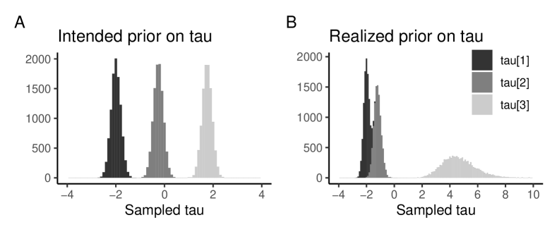
Figure 3: Realized prior of ordered thresholds can be substantially different than intended

Note. Priors were simulated with $N=10000$ plotted as a stacked histogram (binwidth=0.10). A. The intended informative prior on all three thresholds; B. Realized prior on the ordered threshold. Intending to specify the informative priors $\tau_{1}\sim\text{Normal}(-2.00,0.20)$, $\tau_{2}\sim\text{Normal}(-0.25,0.20)$, and $\tau_{3}\sim\text{Normal}(1.75,0.20)$ on the three ordered thresholds but failing to account for the sequential exponents results in drastically different realized priors with $E[\tau_{1}]\approx-2.00$, $E[\tau_{2}]\approx-1$, and $E[\tau_{3}]\approx 4.50$.

Threshold Priors – Induced-Dirichlet

Betancourt, (2019) discussed an “Induced-Dirichlet” prior for ordered thresholds in ordered logistic regression. The prior was designed to produce robust inferences across a wider range of observed data characteristics, namely, sparse responses. The prior is placed on all the thresholds simultaneously, resulting in a regularizing prior, which limits the likelihood of extreme values for the thresholds occurring in the posterior distributions. The nontrivial prior is as follows.

As described by Betancourt, (2019), let $C_{i}$ be the number of response categories for item i then an item will have $C_{i}-1$ threshold parameters ($\bm{\tau}=[\tau_{1},\ldots,\tau_{(C_{i}-1)}]$) to estimate. The threshold parameters define a simplex, or a vector of probabilities that sum to 1; that is, $\bm{P}=[P_{1},P_{2},\ldots,P_{(C_{i})}]$ where $\sum_{c=1}^{C_{i}}P_{c}=1$. The proposed prior maps these probabilities with the latent response variable to regularize the thresholds indirectly through regularizing the vector of probabilities. In this study, the mapping is accomplished using the normal CDF, $\Phi(.)$, and inverse normal CDF, $\Phi^{-1}(.)$. Therefore, the probability distribution is induced by the mapping of $\tau\rightarrow P$, resulting in probabilities defined as

$$P_{1} =\Phi(\tau_{1})$$

$$P_{2} =\Phi(\tau_{2})-\Phi(\tau_{1})$$

$$\vdots$$

$$P_{C_{i}-1} =\Phi(\tau_{C_{i}-1})-\Phi(\tau_{C_{i}-2})$$

$$P_{C_{1}} =1-\Phi(\tau_{C_{i}-1}).$$

The transformation from thresholds to probabilities requires an adjustment to the density function through the Jacobian matrix of partial derivatives. The reparameterization from thresholds to probabilities results in a change in the general density being sampled which can, in turn, alter inferences if the adjustment to the calculated density is not accounted for (see Carpenter, 2017, for an excellent discussion of change of variables and Jacobian adjustments). The adjustment, in this case, follows taking the determinant of the Jacobian matrix. The partial derivatives come from taking the derivative of normal CDF with respect to the threshold parameters. Defining the partial derivative as $\Phi^{\prime}(.)$, for ease of discussion, the Jacobian matrix reduces to

$$J(\bm{\tau}_{i})=\begin{pmatrix}1&\Phi^{\prime}(\tau_{1})&0&\cdots&0\\ 1&-\Phi^{\prime}(\tau_{1})&\Phi^{\prime}(\tau_{2})&\cdots&0\\ 1&0&-\Phi^{\prime}(\tau_{2})&\cdots&0\\ \vdots&\vdots&\vdots&\ddots&\vdots\\ 1&0&0&\cdots&-\Phi^{\prime}(\tau_{C_{i}-1})\end{pmatrix}.$$

The probability density function combining the (1) Dirichlet prior for the probabilities given the thresholds and (2) the Jacobian adjustment for the change of variables from thresholds to probabilities results in the reduced form of

$$Pr(\bm{\tau}|\bm{\alpha})=\text{Dirichlet}(\bm{p}(\bm{\tau})|\bm{\alpha})\times|J(\bm{\tau})|,$$

where $\bm{\alpha}=(\alpha_{1},\alpha_{2},\ldots,\alpha_{C_{i}})$ and $|J(\bm{\tau})|$ represents the determinant of the Jacobian matrix above. For more details on the implementation of this prior in Stan, see Appendix 3. The prior on the vector of thresholds $\bm{\tau}$ is known as an induced-prior.

Reconceptualizing the prior regularizes the estimation of the thresholds due to the constraints placed on the underlying probabilities through the Dirichlet distribution. Modifying the values in the hyperprior vector $\bm{\alpha}$ provides differing degrees of regularization. For example, with four response categories, a uniform prior over the response probabilities is obtained using $\bm{\alpha}=(1,1,1,1)$ and provides equal weight to each response category. Modifying the vector to $\bm{\alpha}=(1,2,2,1)$ induces a greater weight to the middle response categories than either extreme thus increasing the distance between thresholds. Modifying the vector to $\bm{\alpha}=(2,1,1,2)$ induces a greater weight to the extreme response categories thus decreasing the distance between thresholds. The more prior weight given to the extreme response categories, the greater the regularizing effect the prior has on the posterior distribution of the the extreme thresholds. Examples of alternative hyperpriors $\bm{\alpha}$ with the induced thresholds are illustrated in Figure 4.

Choosing among possible prior specifications can be challenging without an inferential interpretation of the hyperprior parameters $\bm{\alpha}$. One way of interpreting the values of $\bm{\alpha}$ is based on the idea that each value represents a “pseudo”-observation. Specifying $\bm{\alpha}=(1,1,1,1)$ is then saying that in a sample of 4 people, we would expect each person to select a different category. However, specifying $\bm{\alpha}=(10,10,10,10)$ similarly implies equal weight to each category, but now we are saying the equal weight is based on a sample of 40 “pseudo”-observations, thus the prior is given more weight. Interpreting the Dirichlet prior in terms of “pseudo”-observations is common in latent class models (Galindo Garre and Vermunt,, 2006; Depaoli,, 2022) and generalized linear models (Schafer,, 1997). Validating this interpretation is out of scope of this work as our focus is on the estimation and implementation, but future work will aim to provide evidence of the prior equivalent sample size interpretation.

An important difference between this joint induced-Dirichlet prior and the sequential sum of exponential prior discussed previously is the lack of strict ordering of the variance associated with each threshold distribution. The joint prior allows each threshold to have different certainty, with middle thresholds typically being more precise than extreme thresholds. This conceptually aligns with the fact small changes in central thresholds imply larger differences in response probabilities than small changes in extreme thresholds.

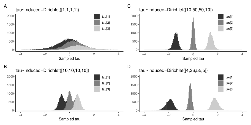
Figure 4: Realized prior of ordered thresholds using a joint induced-Dirichlet prior

Note. Priors were simulated with $N=10000$ plotted as a stacked histogram (binwidth=0.05). A. $\bm{\alpha}=(1,1,1,1)$ is our initial suggestion for a relatively uninformative specification of the induced-Dirichlet prior; B. $\bm{\alpha}=(10,10,10,10)$ illustrates that more precision can induced to each thresholds by increasing the weight uniformly; C. $\bm{\alpha}=(10,50,50,10)$ illustrates how greater precision can be induced to the middle threshold only by increasing the the middle weights but not the extremes; and D. $\bm{\alpha}=(4,36,55,5)$ corresponds roughly to a prior which induces the expected values of thresholds to $E[\tau_{1}]\approx-2.00$, $E[\tau_{2}]\approx-0.25$, and $E[\tau_{3}]\approx 1.75$.

Research Questions

The potential specifications of priors for thresholds in item factor analysis are examined in this study. First, using a simulated dataset with known population parameters and items with a response category without endorsement, which threshold prior specification(s) results in an interpretable threshold posterior distribution(s)? We expect that using the induced-Dirichlet prior will result in an interpretable posterior even when a category is not endorse (as intended). A large variance for the sequentially defined priors is expected to yield a very diffuse posterior for the threshold without endorsement as no information reigns in the extreme values.

Secondly, under what conditions do the different prior structures perform optimally in terms of posterior convergence, credible interval coverage, and widths of credible intervals (i.e., efficiency)? Again, the induced-Dirichlet prior is expected to perform well under all conditions even those with messy data characteristics (e.g., missing cells). In the conditions when respondents sufficiently endorse all categories, we expect each prior specifications to perform well.

Lastly, we demonstrate the effects of using different prior structures in a multiple group item factor analysis. We compare the resulting thresholds of items between groups on items where one group did not endorse a category.

Methods

This study employs simulation methods in two parts and an applied example. First, a single dataset is generated based on the model described in the Model Specification section with a relatively small sample size of 150; the lower end of sample sizes was selected from an review of confirmatory factor analysis (CFA) applications (Padgett,, 2022). The dataset was checked to ensure that items contained a response category with no endorsement. The model is estimated using the prior structure defined in the Model Prior section and using three alternative priors for the thresholds: (1) sequential log-normal with a standard deviation of 1.5, (2) sequential log-normal with a standard deviation of 10000, and (3) Induced-Dirichlet with $\alpha=(1,1,\ldots,1)$. The parameter estimates of each model were evaluated to investigate differences among the posterior distributions of thresholds using the three different prior structures.

Secondly, a Monte Carlo simulation study is conducted to evaluate the estimation performance of the proposed prior structure compared to the existing parameterizations. The proposed design of the Monte Carlo simulation systematically varies the distribution of the indicators (i.e., symmetric of category endorsement), the number of response categories (i.e., 3, 4, 5, 6), and sample size (i.e., 150, 500). The proposed set of response distribution conditions is shown in Figure 5. For the sparse category condition, three additional conditions were added: 1) all items contain a category without endorsement, 2) half of all items are simulated with a category without endorsement, and 3) each factor contains one item with a category without endorsement. The non-sparse items in these conditions were simulated using the asymmetric distribution condition. The number of response categories and sample size conditions were determined based on a recent literature review by Padgett, (2022) which indicated that these values are commonly observed in applied research in psychological assessment.

The posterior distributions were sampled using Stan with four chains and 2000 iterations per chain. The first 1000 iterations were discarded as warm-up. The results of the simulation will focus on the coverage rates and interval widths of 95% credible intervals for all parameters and posterior convergence measured by the effective sample size and $\hat{R}$. Coverage rates were computed by summarizing the frequency with which the true value lay within the central 95% quantiles of the posterior distributions. The interval widths were computed using the difference between the 97.5-and 2.5 percentiles of the posterior distributions. Evaluating coverage rates and interval widths informed how well the posterior distributions captured the population parameters. Preferred are credible intervals with high coverage rates ($\approx$95%) with shorter average interval widths. The results of the Monte Carlo simulation were summarized averaging over conditions to obtain the average coverage rates and the average credible interval widths across conditions. The complete results describing convergence, coverage rates, and credible interval width are reported our supplemental material.

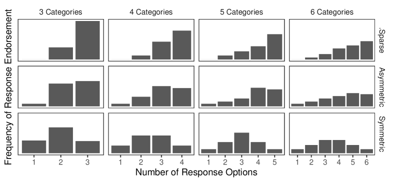
Figure 5: Category response distributions simulated in Monte Carlo study

Data sources

In the applied example, we demonstrate the effects of sparse response categories in testing approximate measurement invariance of thresholds. We used a subset of data from the 2022 Gallup World Poll, looking in particular at a module of eight items centered on balance and harmony (see Lomas et al.,, 2022, , for details on the development of the module), which are integral to well-being and flourishing more broadly (Lomas,, 2021). The survey usually takes 15-20 minutes to complete, featuring around 60 – 80 items (with the number varying among respondents based on screener questions, filters and skip patterns), and involves nationally representative, probability-based samples among the adult populations, aged 15 and older, of around 1,000 people per country (with some larger countries having between 2,000-3000, and some smaller countries having only 500). This sample size is intended to allow, after accounting for the survey weights, a maximum confidence interval of approximately four percentage points, providing enough power ($\beta=0.80,\alpha=.05$) to detect a group difference of approximately nine percentage points. Our analysis specifically focused on differences in balance and harmony between the United States sample (N = 1006) and the Norway sample (N = 1002).

Most items in the poll have binary yes/no response options, although psychometric surveys tend to have Likert-type scales, which allow more nuanced responding patterns and statistical analysis. Gallup has found through experience that yes/no items work better in the context of their international surveys for numerous reasons, including being easier for some participants to understand and being more readily standardized across cultures. To the latter point, for instance, cross-cultural variation has been observed in the way people from different cultures respond to Likert scales. For example, people in more individualistic societies seem to show a preference for response options at the extremes, potentially because it allows them to stand out personally, whereas people in more collectivistic societies hew more towards the center perhaps for the opposite reason (Oishi,, 2010). However, in the balance and harmony module, Gallup was keen to explore the viability of a Likert framework, albeit one still adapted for their cross-cultural research context. First, items were framed in terms of time/frequency (i.e., how often people experience a given state) rather than size/amount (i.e., how much do they experience), as the latter might be somewhat abstract and harder for participants to envision. Second, a four-option scale was used (i.e., always, often, rarely, never) to minimize the complication with the frame. (Note. three-option response scale was not viable informed by Gallup’s experience with people often choosing the middle category).

In the applied example, we demonstrate the effects of sparse response categories in testing approximate measurement invariance of thresholds. We used a subset of data from the Gallup World Poll 2021 wave for comparing the measurement of Balance and Harmony (aspects of well-being and flourishing) between the United States sample and the Norway sample. However, a difficulty in comparing these data are that the response patterns tended to be skewed, leading to items with sparse response distributions and empty categories at the extremes. We therefore used the proposed prior structure to evaluate group comparisons while accounting for the uncertainty in estimation given the sparse response patterns.

Results

Example Analysis of Single Simulated Dataset

The resulting credible intervals (CI) of the posterior distributions of the thresholds of items one and eight across the three prior specifications are shown in Table 1. The major differences in the posterior distribution for the first threshold are of particular attention. An uninformative prior resulted in the posterior of the first threshold being quite wide, given that the observed data did not update the prior meaningfully. On the other hand, the difference between the resulting CI for the Induced-Dirichlet prior compared to the Normal(0,1.5) prior appears negligible. Despite the similarity in the posterior distributions for the two relatively informative priors, differences may exist in sampling efficiency, which the Monte Carlo simulation study will help to tease apart.

Table 1: Posterior distribution of model results among three prior structures

	Induced-Dirichlet			Small Variance			Large Variance			PML
	Mean	LL	UL	Mean	LL	UL	Mean	LL	UL	Est. (SE)
Item 1 Thresholds
$\tau_{11}$	$-$3.41	$-$5.16	$-$2.36	$-$3.25	$-$4.44	$-$2.38	$-$93.7	$-$374.4	$-$3.07	$\ast$
$\tau_{12}$	$-$1.80	$-$2.27	$-$1.42	$-$1.92	$-$2.41	$-$1.50	$-$1.97	$-$2.46	$-$1.54	$-$2.20 (0.25)
$\tau_{13}$	$-$0.11	$-$0.35	0.13	$-$0.19	$-$0.42	0.06	$-$0.23	$-$0.49	0.01	$-$0.25 (0.14)
Item 8 Thresholds
$\tau_{81}$	$-$3.89	$-$5.67	$-$2.71	$-$3.72	$-$5.08	$-$2.70	$-$127.2	$-$507.4	$-$5.41	$\ast$
$\tau_{82}$	$-$1.90	$-$2.45	$-$1.45	$-$2.05	$-$2.66	$-$1.54	$-$2.33	$-$3.23	$-$1.72	$-$2.31 (0.35)
$\tau_{83}$	$-$0.03	$-$0.31	0.27	$-$0.13	$-$0.43	0.17	$-$0.21	$-$0.57	0.12	$-$0.21 (0.17)

• Note. $\ast$Parameter not estimated by lavaan due to no responses observed in category 1. Mean = Posterior mean; LL = posterior 2.5%-tile; UL = posterior 97.5%-tile; PML Est. = Pairwise Maximum Likelihood Point Estimate from lavaan (Rosseel,, 2012). Small Variance = $\text{Normal}(0,1.5)$ default prior in blavaan (Merkle et al.,, 2021). Large variance=$\text{Normal}(0,10^{5})$ default prior in Mplus (Asparouhov and Muthen,, 2010).

Monte Carlo Simulation

Posterior convergence

Posterior convergence was assessed using the effect sample size and Gelman-Rubin-Brooks convergence criteria, $\hat{R}$. Averaging over all parameters and conditions, the joint induced-Dirichlet prior resulted in an average $\hat{R}=1.007$ with 98.7% of estimates below 1.1 and an average effective sample size of 2479. The small variance prior resulted in an average $\hat{R}=1.004$ with 99.4% of estimates below 1.1 and an average effective sample size of 2470. The large variance prior resulted in an average $\hat{R}=1.148$ with 64.2% of estimates below 1.1 and an average effective sample size of 864. The large variance prior distribution resulted in significantly poor summary estimates of convergence compared to the smaller variance prior under these conditions (OR=0.01). The posterior distributions converged on average except under the large variance prior.

Of special interest in this study are the posterior distributions for the thresholds. Summaries of the threshold parameter convergence criteria across prior distributions and response distributions are given in Table 2. An asymmetric or symmetric response distribution resulted in adequate convergence regardless of prior choice, but if even one item is sparsely endorsed the small variance or joint prior converged much better than the large variance prior. In summary of convergence, the difference between the joint induced-Dirichlet and small variance successive sum prior was negligible, but the large variance successive sum prior converged poorly.

Table 2: Convergence of threshold posterior depended on the distribution of observed indicators and prior specification

Distribution	Prior	Avg. $\hat{R}$	% $\hat{R}<1.1$	Avg. ESS
Sparse	Joint	1.006	98.7	2890.4
	Small Variance	1.002	99.8	2892.2
	Large Variance	1.190	54.5	147.7
Asymmetric	Joint	1.001	99.9	2674.0
	Small Variance	1.001	99.9	2666.4
	Large Variance	1.002	99.7	2539.9
Symmetric	Joint	1.002	99.7	2959.5
	Small Variance	1.003	99.7	2888.9
	Large Variance	1.003	99.5	2841.7

• Note. Joint = joint induced-Dirichlet prior; Small Variance = $\text{Normal}(0,1.5)$; Large variance=$\text{Normal}(0,10^{5})$; Avg. ESS = average effective sample size.

Posterior coverage

The coverage rates of the posterior credible intervals is considered next. Averaging over all conditions and parameters except the fixed threshold parameters, coverage rates below the nominal level 0.95 for each prior structure were: 0.757 for the joint prior, 0.789 for the small variance prior, and 0.784 for the large variance prior. Across conditions and parameters, the coverage rates for the prior specifications varied from 0.13 to 0.99 for the joint prior, 0.14 to 0.99 for the small variance prior, and 0.15 to 0.99 for the large variance prior. The high variability in coverage rates among conditions and parameters indicates that coverage is potentially problematic regardless of prior specification when sample sizes are 500 or less.

The coverage rates varied substantially among conditions, and we identified substantial differences in coverage occurred among the different response distributions (Table 3). We found negligible differences in the coverage rates and average credible interval widths across the prior specifications within in the symmetric and asymmetric response distribution conditions for all parameters. However, excluding the fixed thresholds, the CI coverage was significantly worse in the asymmetric (OR = 0.84) and sparse (OR = 0.07) response distributions compared to the symmetric response distribution conditions. This pattern was consistent across all number of response categories conditions. Within the sparse response distribution conditions, we found the number of items that contained a empty response category had a major impact on the coverage rates.

Posterior CI widths

The average widths are reported in Table 3. The average CI widths were consistent across priors specifications within the symmetric and asymmetric response distribution conditions for each parameter. We found substantial difference in the CI widths across prior specifications in the sparse response distribution conditions. The magnitude of the difference in CI width depended on the parameter and number of sparse items, which we focus on next.

Factor loading CI widths were approximately the same in the joint and small variance threshold prior specifications. The CI widths for factor loadings was noticeably narrower in the large variance threshold prior specifications regardless of the number of sparse items. However, the coverage rate for factor loadings also tended to be slightly lower for the large variance specifications compared to the other prior specifications. Resulting in a trade-off between the coverage and interval widths depending on the prior specification for threshold parameters.

The factor variance patterns had a similar pattern of CI widths and coverage compared to the factor loadings. The difference between these two parameters was that the difference in interval widths was less drastic. The factor covariances tended to have similar CI widths but difference coverage rates across Sparse response distribution conditions.

The threshold parameters highlight the severe differences among the CI widths between prior specifications. For the non-fixed threshold parameters, the CI widths were similar across prior specifications when two or six sparse items were present. When all twelve items contained sparse response distributions, the large variance prior had wider CIs than the small variance prior. However, for the fixed threshold separating the empty response category and the next category, the large variance prior had impractical CI widths regardless of the number of sparse items. In the conditions with only two sparse items, the average CI width of the threshold posterior was over 76 units. The widths under the joint induced-Dirichlet or small variance prior were more reasonable between 2-3. This result highlights how even a marginally informative prior with a reasonable variance can significantly impact the posterior distribution when the data contain a category without endorsement.

Table 3: Posterior coverage and CI width depended on prior and response distribution

Distribution		Coverage Rate (%)			Avg CI Width
(# Sparse Items)	Parameter	Joint	Small Variance	Large Variance	Joint	Small Variance	Large Variance
Symmetric (0)	Loadings	93.7	93.4	92.9	0.680	0.686	0.688
	Factor Variances	92.2	92.0	92.5	0.908	0.927	0.941
	Factor Covariance	90.9	90.5	90.6	0.291	0.297	0.299
	Thresholds	94.8	94.1	94.4	0.55.1	0.565	0.574
Asymmetric (0)	Loadings	94.2	94.1	93.5	0.746	0.746	0.756
	Factor Variances	89.6	90.1	90.1	0.968	0.969	1.003
	Factor Covariance	89.5	90.3	89.8	0.304	0.303	0.308
	Thresholds	90.3	94.1	94.6	0.581	0.592	0.618
Sparse (2)	Loadings	91.9	91.8	93.1	0.862	0.858	0.313
	Factor Variances	86.9	87.5	85.0	0.954	0.946	0.811
	Factor Covariance	84.0	81.4	78.2	0.282	0.278	0.269
	Thresholds	88.9	93.8	92.6	0.581	0.594	0.515
	Fixed Threshold∗	∗	∗	∗	3.212	2.128	56.760
Sparse (6)	Loadings	93.5	93.3	92.9	0.825	0.822	0.299
	Factor Variances	87.9	88.3	77.8	0.968	0.966	0.748
	Factor Covariance	88.8	88.4	80.0	0.298	0.294	0.278
	Thresholds	87.8	93.5	92.5	0.578	0.590	0.520
	Fixed Threshold∗	∗	∗	∗	2.891	2.149	44.505
Sparse (12)	Loadings	94.5	94.3	91.9	0.925	0.927	0.289
	Factor Variances	86.0	85.4	76.5	1.008	0.996	0.722
	Factor Covariance	85.4	83.5	76.3	0.308	0.296	0.272
	Thresholds	19.6	14.8	16.2	1.171	0.995	1.200
	Fixed Threshold∗	∗	∗	∗	2.892	2.169	11.345

• Note. ^∗Fixed threshold was set to $-15$ for simulating a “sparse”/empty response category and credible intervals for this threshold should NOT contain the simulating parameter. Joint = joint induced-Dirichlet prior; Small Variance = $\text{Normal}(0,1.5)$; Large variance=$\text{Normal}(0,10^{5})$.

Indicator variable effect

In our initial plan of conditions in the simulation study, we set the sparse response distribution conditions to always use an item with an empty response category as the indicator variable. After we investigated the coverage and direction of mis-coverage (positive vs. negative bias) for parameters, we identified that the factor variance parameters were consistently underestimated in the sparse response distribution conditions. Our hypothesis was that using a variable with a more restricted range may cause underestimation. To counter this potential issue, we reran conditions with a sparse response category for half the items and flipped which item was used as the indicator variable to a nonsparse item.

Table 4: Using an indicator variable with an empty response category results in poorer coverage

Parameter	Indicator Variable	Joint	Small Variance	Large Variance
Coverage Rate (%)
Loading	Sparse	92.3	92.0	93.1
	Non-sparse	94.6	94.7	92.8
Factor Variance	Sparse	85.6	85.9	80.8
	Non-sparse	90.3	90.7	75.0
Factor Covariance	Sparse	87.8	86.9	78.4
	Non-sparse	89.8	89.9	81.4
Thresholds	Sparse	86.2	92.9	92.3
	Non-sparse	89.2	94.0	92.7
Fixed Threshold	Sparse	∗	∗	∗
	Non-sparse	∗	∗	∗
Avg. CI Width
Loading	Sparse	0.891	0.891	0.292
	Non-sparse	0.758	0.754	0.305
Factor Variance	Sparse	0.955	0.950	0.747
	Non-sparse	0.981	0.981	0.748
Factor Covariance	Sparse	0.286	0.279	0.276
	Non-sparse	0.311	0.309	0.280
Thresholds	Sparse	0.576	0.589	0.525
	Non-sparse	0.579	0.591	0.516
Fixed Threshold	Sparse	2.893	2.154	98.446
	Non-sparse	2.891	2.147	28.134

• Note. ^∗Fixed threshold was set to $-15$ for simulating a “sparse”/empty response category and credible intervals for this threshold should NOT contain the simulating parameter. Joint = joint induced-Dirichlet prior; Small Variance = $\text{Normal}(0,1.5)$; Large variance=$\text{Normal}(0,10^{5})$.

The coverage rates and CI widths comparing the sparse and non-sparse are shown in Table 4. We found that using an indicator variable with an empty response category consistently resulted in poorer coverage rates for most parameters. The CI widths for factor loadings tended to be narrower when a non-sparse item was used, but the CI widths did not substantially differ for the other parameters. The sole exception was the CI width for the fixed threshold.

Gallup World Poll

Norway and the United States are relatively comparable countries in terms of developmental status, and one might not generally expect any differences in the operating characteristics of the assessment tool across these two countries. The assessment of balance and harmony could be revealing as to potential nuanced differences in the flourishing of these two countries. Indeed, it is intriguing that across the 8 items, if we take the percentage of respondents in each country that report experience the various aspects of balance and harmony either “always” or “often,” while Norway does better overall (with higher levels of flourishing than the USA on 6 items), the USA nevertheless fares better on two of them. These include: amount of things happening in life is “just right” (Norway ranks 33rd out of 141 countries, with 72.7% answering either “always” or “often,” versus USA at 25th with 74.3%); life in balance (Norway at 13th with 81.8% versus USA at 51st with 70.8%); harmony with those around (Norway at 3rd with 96.3% versus USA at 29th with 91.1%); thoughts and feelings in harmony (Norway at 12th with 88.1% versus USA at 26th with 80.0%); feel stable and secure (Norward at 3rd with 93.1% versus USA at 18th with 89.0%), content (Norway 13th with 90.4% versus USA at 27th with 86.5%); mind at ease (Norway at 27th with 81.3% versus USA at 49th with 75.9%); and inner peace (Norway at 47th with 73.4% versus USA at 24th with 79.1%).

However, such nuances aside, the sum of responses (total score) by individuals is not significantly different on average between countries ($t(1878.2)=0.91,p=.418$). Once we dive into the data we see that the item “Harmony Around” (You Are in Harmony With Those Around You), we see that the Norway sample did not endorse Never (see Table 5). Leading to a sparse response distribution that would limit our ability to compare the invariance of the measurement properties more thoroughly. As mentioned in the introduction, we could collapse the categories of Never and Rarely into one category then collapse Often and Always into another. However, collapsing categories and retesting the difference in total score changes our interpretation from “no difference” to a “significance difference” ($t(1935.6)=2.9804,p=.002$). A dependence of interpretation based solely on how the responses are coded is not ideal, and this issue becomes exacerbated when one moves to analyzing all the countries simultaneously.

Comparing the measurement properties between these two countries using the original response scale (Never to Always) is preferred so as not to induce a difference between countries artificially. Using the methods developed earlier in this work, we estimated a multi-group item factor model to compare the thresholds between countries. The invariance of some of the thresholds was dependent upon how the model was estimated. In one extreme using pairwise maximum likelihood (PML), the invariance of threshold one could not even be assessed for the “Harmony Around” item because the estimator of the threshold does not exist within the Norway sample. In another extreme using a “flat prior”, Normal(0, $10^{5}$), for the thresholds, the posterior distribution did not converge to a realistic distribution within 2000 iterations with four different chains. Somewhere in the middle are the results we focus on next.

Table 5: Response distribution of balance and harmony items in Norway and US samples

	Norway				United States
Item	Never	Rarely	Often	Always	Never	Rarely	Often	Always
Balance	11	166	703	96	44	241	554	137
Amount Right	28	237	601	110	58	194	561	163
Harmony Around	0	36	753	187	14	71	673	218
Thoughts Harmony	10	105	750	111	19	119	667	171
Stable	7	50	470	449	21	85	520	350
Content	8	85	754	129	31	101	592	252
Mind Ease	17	163	655	141	52	182	611	131
Inner Peace	27	234	610	105	29	172	584	191
Total Score	24.0 (3.10)				23.9 (3.78)

• Note. Never=1, Rarely=2, Often=3, and Always=4; $t$-test comparing total (sum) score between countries was nonsignificance ($t(1878.2)=0.91,p=.42$).

The posterior distributions of the thresholds are summarized in Table 6. The first threshold posteriors for the Norway sample are generally lower than the US sample’s except for items Stable and Inner Peace that were nearly identical. The differences among these samples’ estimated thresholds were less obvious for the second and third thresholds. These results suggest that the individuals in the Norway sample were less likely to endorse the lowest response category compared to individuals in the US sample. Of particular interest in this study was the difference in posterior distribution for the thresholds of item 3 (Harmony Around), and the posteriors are shown in Figure 6. We were particularly interested in how sensitive the difference in estimated thresholds were to prior specification. Three different prior specifications were used to show how sensitive the posteriors were to choice of prior. The Norway sample’s first threshold was most sensitive to the prior. Using a default, relatively uninformative prior of $\alpha=[1,1,1,1]$ for the induced-Dirichlet specification resulted in posteriors that were nearly identical to the sequential exponential of normal distribution priors that is the default in blavaan. In both specifications, we would conclude that the first threshold differs between Norway and the US. However, if one modifies the induced-Dirichlet prior to $\alpha=[10,10,10,10]$, supplying the intended equivalent of 10 observations per response category, then differences between samples decrease significantly even though no observations were observed endorsing the lowest response category for the Norway sample.

Table 6: Posterior distribution of thresholds in multi-group item factor model

		$tau[1]$			$tau[2]$			$tau[3]$
Item	Country	Mean	SD	Q(2.5%, 97.5%)	Mean	SD	Q(2.5%, 97.5%)	Mean	SD	Q(2.5%, 97.5%)
Balance	Norway	-3.41	0.19	(-3.80, -3.05)	-1.32	0.08	(-1.48, -1.16)	1.93	0.10	(1.74, 2.13)
	US	-2.01	0.09	(-2.18, -1.84)	-0.66	0.05	(-0.76, -0.56)	1.32	0.07	(1.19, 1.46)
Amount Right	Norway	-2.13	0.09	(-2.32, -1.95)	-0.67	0.05	(-0.76, -0.57)	1.36	0.06	(1.24, 1.48)
	US	-1.75	0.07	(-1.89, -1.60)	-0.72	0.05	(-0.82, -0.63)	1.10	0.06	(0.99, 1.21)
Harmony Around	Norway	-4.24	0.65	(-5.76, -3.31)	-2.08	0.09	(-2.27, -1.90)	1.01	0.05	(0.90, 1.12)
	US	-2.63	0.13	(-2.89, -2.38)	-1.61	0.07	(-1.75, -1.47)	0.91	0.06	(0.80, 1.02)
Thoughts Harmony	Norway	-4.55	0.32	(-5.23, -3.97)	-2.17	0.14	(-2.47, -1.90)	2.23	0.15	(1.95, 2.54)
	US	-3.51	0.19	(-3.90, -3.14)	-1.73	0.10	(-1.94, -1.54)	1.53	0.09	(1.35, 1.72)
Stable	Norway	-3.31	0.19	(-3.71, -2.96)	-2.10	0.10	(-2.31, -1.91)	0.15	0.05	(0.05, 0.25)
	US	-3.23	0.16	(-3.56, -2.92)	-1.95	0.11	(-2.16, -1.76)	0.57	0.07	(0.44, 0.71)
Content	Norway	-4.07	0.26	(-4.59, -3.58)	-2.14	0.13	(-2.40, -1.90)	1.82	0.11	(1.61, 2.03)
	US	-3.12	0.16	(-3.45, -2.82)	-1.83	0.11	(-2.05, -1.63)	1.08	0.08	(0.93, 1.25)
Mind Ease	Norway	-4.07	0.27	(-4.62, -3.60)	-1.59	0.11	(-1.82, -1.39)	1.93	0.12	(1.70, 2.19)
	US	-2.78	0.14	(-3.07, -2.52)	-1.19	0.09	(-1.36, -1.02)	1.92	0.11	(1.72, 2.15)
Inner Peace	Norway	-2.81	0.14	(-3.09, -2.55)	-0.85	0.07	(-0.98, -0.72)	1.77	0.09	(1.60, 1.95)
	US	-2.71	0.12	(-2.96, -2.47)	-1.12	0.07	(-1.26, -0.99)	1.21	0.07	(1.07, 1.35)

• Note. $N_{Norway}=976$, $N_{UnitedStates}=976$. All posteriors above are based on specifying the induced-Dirichlet prior with $\alpha=[1,1,1,1]$.

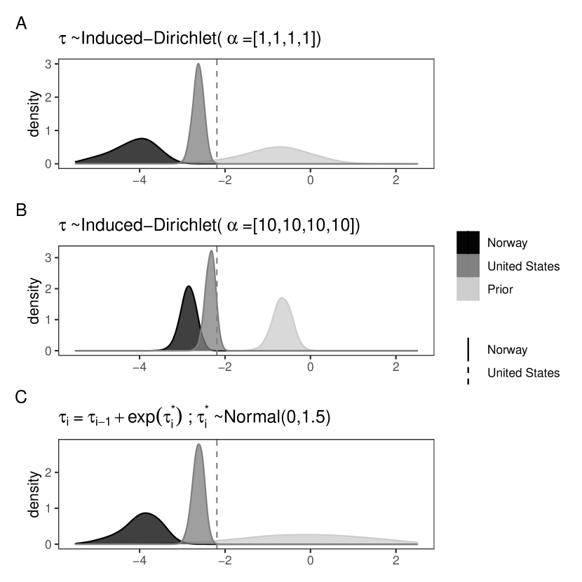
Figure 6: Comparison of Harmony Around item threshold posterior distribution among prior specifications

Note. Vertical line represent the estimated thresholds under pairwise maximum likelihood (PML in lavaan). The threshold, tau[1], estimator does not exist for Norway under PML so the line is not present. Solid line is for the Norway estimated thresholds and the dashed line is for the US estimated thresholds.

Discussion

The prevalence of questionnaires using ordered categorical responses in social and behavioral science calls for a robust understanding and set of tools for the most appropriate ways of analyzing such data. Although the importance of appropriate analysis has a statistical foundation, the ultimate goal of much, if not most, social science research is to make defensible and reasonable decisions about the constructs being evaluated. Such decisions can affect the lives of individuals, families, communities, and society at large, so every effort must be taken to ensure that strong evidence supports the use of data collection instruments. Of course, the evidence supporting an instrument’s use for a particular purpose can take many forms. Still, the evidence yielded by latent variable models, such as those described in this paper, is one such piece of evidence. The results of this study will contribute to the extant literature on appropriate modeling techniques to support decision-making in social and behavioral science when researchers use categorical response options as part of their assessment procedure.

The present analyses provide the first evaluation within a latent variable modeling tradition of the effects of a joint threshold prior specification on parameter estimation, at least to the best of our knowledge. Our results were partially consistent with results from a frequentist estimation tradition with respect to the effects of sparse response distribution on parameter recovery. Our results aligned with the conclusions of bias of factor loadings and factor correlations (DiStefano and Morgan,, 2014; DiStefano et al.,, 2021) when many items contain a sparse response distribution (e.g., a type of nonnormality). Our results depart from prior conclusions that modeling sparse leads to poor estimation performance (Savalei,, 2011; DiStefano et al.,, 2021). We found that the estimation performance under a Bayesian estimation procedure avoids, at least a degree, the complex issues that arise when estimating polychoric correlations. For instance, Savalei, (2011) demonstrated how parameter and standard error estimation deteriorates when a cell of response categories is empty. We saw some of these concerns with lower than nominal coverage rates of credible intervals when a sparse item was used as the indicator variable, but shifting to a different indicator variable significantly improved performance. The use of Bayesian estimation with threshold priors that default to realistic values for the threshold appears to be a potentially viable solution.

The specification of priors for latent variable models is an ongoing area of research (Depaoli,, 2022; Miočević et al.,, 2021; Zitzmann et al.,, 2020; van Erp et al.,, 2018). The attention of much of this research is on the specification of the priors for the latent variables or the latent regression parameters. Similarly, the item response theory literature has a long history of the evaluation of priors for latent variables. One aspect the broader latent variable modeling literature on prior specification can take away from the IRT literature is the use of joint priors for item parameters (e.g., van der Linden et al.,, 2010). The proposed Dirichlet prior for threshold incorporates the joint prior specification for item parameters with the interpretative goals of priors for latent variables.

The intended interpretation of the Dirichlet prior for the threshold is as the number of “pseudo”-observations endorsing each response option. As evidenced by the Gallup World Poll Harmony module application, the intended interpretation of pseudo-counts provides a valuable inferential tool for explaining how and why the posterior distribution is sensitive to prior specification. Simply supplying the equivalent of one observation endorsing the first response category was not enough to reduce the difference between groups on the first threshold, but supplying the equivalent of ten observations reduced the difference noticeably. So not only can the proposed induced-Dirichlet prior specification help meaningfully specify the model, but the prior can help regularize the estimates of extreme thresholds when no endorsement is observed. At this point, we think interpreting the hyperparameter $\alpha$ as pseudo-counts seems reasonable. However, this can be empirically evaluated (Morita et al.,, 2008, 2012). Evaluating the prior effective sample size would be valuable to identify if the interpretation of pseudo-counts is appropriate.

The applied example of a multiple-group model highlighted the effects of prior specification on posterior comparisons. Multiple group models are commonly used to help test the invariance of model parameters, and more work on the effects of prior specification needs to be considered in these types of models. Previous research has shown how collapsing categories can lead to different conclusions about invariance, e.g., “… collapsing also led to rejecting the assumption of slope equality in spite of a commensurate data-generating model.” (Rutkowski et al.,, 2019). Conclusions being dependent on how the categories were collapsed is not ideal and, as Rutkowski and colleagues pointed out, could lead to issues of “p-hacking” (Simmons et al.,, 2011; Simonsohn et al.,, 2014). The methods we described in this work could be a meaningful solution to this issue, and the region of practical equivalence (ROPE, Shi et al.,, 2019) approach to invariance testing could be relatively easily utilized by incorporating the proposed prior structure.

Recommendations

The results of these studies highlight the importance of how observed data characteristics can negatively influence the estimation of Bayesian factor models. When at least one item contains an empty response category, the estimates of all parameters are impacted to some degree. We first recommend making sure not to use an item with an empty category as the reference indicator. Secondly, when estimating a single group, single time point factor model, the difference between using a small variance prior for thresholds versus the proposed joint induced-Dirichlet prior were negligible. We found that using either approach will yield credible intervals with good coverage rates for most parameters under the conditions in this study.

Comparing threshold parameters between groups is less certain when the number of thresholds vary because of empty categories. The example applied analysis showed how the uncertainty of observing an empty category can be taken into account without restricting the range of the observed data to force an equal number of categories. However, this is not yet easily implemented in blavaan or Mplus. We think based on the results of this study, such an approach can more accurately model categorical data in latent variable modeling without modifying the characteristics of the observed data.

Conclusion

Modeling messy data can require difficult analytic decisions including transforming the observed data or developing more complex methods to account for the messiness. We demonstrated an approach to estimating thresholds in Bayesian item factor analysis that accounts for the inherent messiness in data commonly encountered in social science research. Researchers can utilize the regularizing joint prior on thresholds to account for small sample sizes or heavily skewed response distributions to better estimate their models with confidence that their results are less influenced by messy data characteristics.

Acknowledgments

The authors would like to thank Roy Levy from Arizona State University for helpful comments on an earlier draft of this paper presented at the American Educational Research Association annual meeting.

1 Sampling Latent Response Distribution

The following Stan code is based on the implementation of Goodrich, (2017).

⬇

//y = observed response vector

//mu = latent response mean vector (if marginal likelihood, then this is 0

//L = lower Cholesky decomposition of covariance matrix of latent responses

//b = matrix (nitems by nlevs) of thresholds

//u = nuisance (0,1) variable

//nlevs = vector designating number of levels/number of categories for each item

vector[] tmvn(int[] y, vector mu, matrix L, vector[] b, real[] u, int[] nlevs) {

int K = rows(mu);

vector[K] d;

vector[K] z;

vector[K] out[2];

for (k in 1:K) {

int km1 = k - 1;

real nu;

if (y[k] == 1) {

real z_star = (b[k,1] - (mu[k] + ((k > 1) ? L[k,1:km1] * head(z, km1) : 0))) / L[k,k];

real u_star = Phi(z_star); //normal CDF for implied density of TMVN

nu = u_star * u[k];

d[k] = u_star;

} else if(y[k] == nlevs[k]) {

real z_star = (b[k,(nlevs[k]-1)] - (mu[k] + ((k > 1) ? L[k,1:km1] * head(z, km1) : 0))) / L[k,k];

real u_star = Phi(z_star);

d[k] = 1 - u_star;

nu = u_star + d[k] * u[k];

} else {

int lb = y[k]-1;

int ub = y[k];

real z_starL = (b[k,lb] - (mu[k] + ((k > 1) ? L[k,1:km1] * head(z, km1) : 0))) / L[k,k];

real z_starU = (b[k,ub] - (mu[k] + ((k > 1) ? L[k,1:km1] * head(z, km1) : 0))) / L[k,k];

real u_starL = Phi(z_starL);

real u_starU = Phi(z_starU);

nu = u_starL + (u_starU - u_starL)*u[k];

d[k] = u_starU - u_starL;

}

z[k] = inv_Phi(nu); //convert back to z-score from uniform variate

}

out[1] = z; //simulated ystar value

out[2] = d; //density

return(out);

}

2 Deriving informative prior for sequentially defined thresholds

Placing informative priors on individuals thresholds is not entirely obvious. For instance, consider the situation with an assessment where items are scored with four ordered categories, and previous results are available to create informative priors for the thresholds. The reported threshold point estimates for one of the items are $-$2.00, $-$0.25, and 1.75. An informative prior for the first thresholds is straightforward,

$$\tau_{1}\sim\text{Normal}(-2.00,0.20).$$

An informative prior for the second threshold is unfortunately not simply $\tau_{2}\sim\text{Normal}(-0.25,0.25)$, but is instead specified relative to threshold 1. The informative prior for $\tau_{2}$ needs to be constructed using the solution to the following system.

1. We need to identify the distribution of $\tau^{\ast}_{2}$ such that $\tau_{2}\sim\text{Normal}(-0.25,0.25)$.

2. Rewrite $\tau_{2}=\tau_{1}+exp(\tau^{\ast}_{2})$ in terms of the expected value and variances of each element, taking advantage of the fact that $exp(\tau^{\ast}_{2})\sim\text{logNormal}(.)$.

   $$E[\tau_{2}] =E[\tau_{1}]+exp\left(E[\tau^{\ast}_{2}]+\frac{Var[\tau^{\ast}_{2}]}{2}\right)$$

   $$Var[\tau_{2}] =Var[\tau_{1}]+\left(exp\left(Var[\tau^{\ast}]\right)-1\right)exp\left(2E[\tau^{\ast}_{2}]+Var[\tau^{\ast}_{2}]\right),\ \tau_{1}\perp\tau^{\ast}_{2},$$

3. The prior we need to specify to obtain the desired $E[\tau_{2}]$ and $Var[\tau_{2}]$ is then the solution system of equations above for values of $E[\tau^{\ast}_{2}]$ and $Var[\tau^{\ast}_{2}]$ under the conditions that $E[\tau_{1}]<E[\tau_{2}]$ and $Var[\tau_{1}]<Var[\tau_{2}]$. The solution is not immediately obvious but is analytically defined.

4. The solution (after some algebra) is

   $$E[\tau_{c}] >E[\tau_{c-1}]$$

   $$Var[\tau_{c}] >Var[\tau_{c-1}]$$

   $$E[\tau^{\ast}_{c}] =log\left(E[\tau_{c}]-E[\tau_{c-1}]\right)-\frac{Var[\tau^{\ast}_{c}]}{2}$$

   $$Var[\tau^{\ast}_{c}] =log\left(\frac{Var[\tau_{c}]-Var[\tau_{c-1}]+exp\left(2log(E[\tau_{c}]-E[\tau_{c-1}])\right)}{exp\left(2log(E[\tau_{c}]-E[\tau_{c-1}])\right)}\right).$$

5. The resulting prior for $\tau^{\ast}_{2}$ one needs to use to obtain the prior we want to place on $\tau_{2}$ is

   $$\tau^{\ast}_{2}\sim\text{Normal}(0.55,0.02).$$

A major caveat is that the resulting prior on $\tau_{2}$ is only approximately normally distributed (the larger the variance of $\tau^{\ast}_{2}$ is, the more asymmetric the prior on $\tau_{2}$ will be), though we will have the desired expected value and variance.

3 Induced-Dirichlet Prior Implementation

The Dirichlet distribution is defined as

$$\text{Dirichlet}(\theta|\alpha)=\frac{\Gamma\left(\sum_{k=1}^{K}\alpha_{k}\right)}{\prod_{k=1}^{k}\Gamma\left(\alpha_{k}\right)}\prod_{k=1}^{K}\theta_{k}^{\alpha_{k}-1},$$ (1)

where $K\in\mathbb{N},\alpha\in(\mathbb{R}^{+})^{K}$, for a $\theta\in K$-simplex. The hyper-parameter vector $\bm{\alpha}$ is strictly positive, with each element $\alpha>0$. Sampling from the Dirichlet distribution produces a vector of probabilities that sum to unity. The probability density function for the Dirichlet distribution can then be used to compute the likelihood of a given vector of probabilities that define a simplex based on the given hyper-parameter for the Dirichlet distribution. In this work, the Dirichlet distribution is used to compute the probability/likelihood associated with a given simplex of probabilities induced by a set of thresholds for an item.

The density function of the Dirichlet distribution provides a convenient mechanism for using the probabilities induced by a set of thresholds for an item. We can randomly sample thresholds indirectly through the Dirichlet distribution. First, the simplex of probabilities are simulated, then thresholds are computed based on the simulated probabilities.

⬇

vector phi_logit_approx_vec(vector b) {

int N = num_elements(b);

vector[N] a;

a = inv_logit( 1.702*b );

return(a);

}

//c = vector of thresholds

//alpha = dirichlet hyper-prior parameters default=rep(1, num_elements(c)+1)

//phi = center of latent response distribution, default=0

real induced_dirichlet_lpdf(vector c, vector alpha, real phi) {

int K = num_elements(c) + 1;

vector[K - 1] anchoredcutoffs = c - phi; //which is first is important c vs. phi...

vector[K] sigma;

vector[K] p;

matrix[K, K] J = rep_matrix(0, K, K);

sigma[1:(K-1)] = phi_logit_approx_vec(anchoredcutoffs);

sigma[K] = 1;

p[1] = sigma[1];

for (k in 2:(K - 1))

p[k] = sigma[k] - sigma[k - 1];

p[K] = 1 - sigma[K - 1];

for (k in 1:K) J[k, 1] = 1;

for (k in 2:K) {

real rho = 1.702 * sigma[k - 1] * (1 - sigma[k - 1]);

J[k, k] = - rho;

J[k - 1, k] = + rho;

}

return dirichlet_lpdf(p | alpha)

+ log_determinant(J);

}

References

- Asparouhov and Muthen, (2010) Asparouhov, T. and Muthen, B. (2010). Bayesian analysis using mplus: Technical implementation. technical report. https://www.statmodel.com/download/Bayes3.pdf.
- Asparouhov and Muthen, (2021) Asparouhov, T. and Muthen, B. (2021). Bayesian analysis of latent variable models using mplus. https://www.statmodel.com/download/BayesAdvantages18.pdf. Accessed: 2023-4-6.
- Bandalos, (2014) Bandalos, D. L. (2014). Relative performance of categorical diagonally weighted least squares and robust maximum likelihood estimation. Structural Equation Modeling: A Multidisciplinary Journal, 21(1):102–116.
- Bearden and Netemeyer, (1999) Bearden, W. O. and Netemeyer, R. G. (1999). Handbook of Marketing Scales: Multi-Item Measures for Marketing and Consumer Behavior Research. SAGE Publications.
- Betancourt, (2019) Betancourt, M. (2019). Ordinal regression. https://betanalpha.github.io/assets/case_studies/ordinal_regression.html.
- Depaoli, (2022) Depaoli, S. (2022). The specification and impact of prior distributions for categorical latent variable models. Structural Equation Modeling: A Multidisciplinary Journal, 29(3):350–367.
- DeVellis, (2016) DeVellis, R. F. (2016). Scale Development: Theory and Applications (Vol. 26). SAGE Publications, Thousand Oaks, CA.
- DiStefano and Morgan, (2014) DiStefano, C. and Morgan, G. B. (2014). A comparison of diagonal weighted least squares robust estimation techniques for ordinal data. Structural Equation Modeling: A Multidisciplinary Journal, 21(3):425–438.
- DiStefano et al., (2021) DiStefano, C., Shi, D., and Morgan, G. B. (2021). Collapsing categories is often more advantageous than modelingsparse data: Investigations in the CFA framework. Structural Equation Modeling: A Multidisciplinary Journal, 28(2):237–249.
- Fink, (2003) Fink, A. (2003). How to design survey studies. Sage.
- Forero et al., (2009) Forero, C. G., Maydeu-Olivares, A., and Gallardo-Pujol, D. (2009). Factor analysis with ordinal indicators: A monte carlo study comparing DWLS and ULS estimation. Structural Equation Modeling: A Multidisciplinary Journal, 16(4):625–641.
- Fowler, (2014) Fowler, F. J. (2014). Survey research methods (5th ed.). Sage.
- Galindo Garre and Vermunt, (2006) Galindo Garre, F. and Vermunt, J. K. (2006). Avoiding boundary estimates in latent class analysis by bayesian posterior mode estimation. Behaviormetrika, 33(1):43–59.
- Garner and Hake, (1951) Garner, W. R. and Hake, H. W. (1951). The amount of information in absolute judgements. Psychological Review, 58(1):446–459.
- Gelman et al., (2013) Gelman, A., Carlin, J. B., Stern, H. S., Dunson, D. B., Vehtari, A., and Rubin, D. B. (2013). Bayesian data analysis. CRC press, Boca Raton, FL, 3rd edition.
- Geweke et al., (1994) Geweke, J., Keane, M., and Runkle, D. (1994). Alternative computational approaches to inference in the multinomial probit model. The Review of Economics and Statistics, 76(4):609–632.
- Goodrich, (2016) Goodrich, B. (2016). Stan examples: Truncated multivariate probit. https://github.com/stan-dev/example-models/blob/master/misc/multivariate-probit/probit-multi-good.stan.
- Goodrich, (2017) Goodrich, B. (2017). Truncated multivariate normal variates in stan. https://00335207212371662729.googlegroups.com/attach/767409563fc2e/tMVN.pdf.
- Jöreskog and Sörbom, (1988) Jöreskog, K. G. and Sörbom, D. (1988). LISREL 7. A guide to the program and applications (2nd ed.). International Education Services.
- Jorgensen et al., (2018) Jorgensen, T. D., Kite, B. A., Chen, P.-Y., and Short, S. D. (2018). Permutation randomization methods for testing measurement equivalence and detecting differential item functioning in multiple-group confirmatory factor analysis. Psychological Methods, 23(4):708–728.
- Lewandowski et al., (2009) Lewandowski, D., Kurowicka, D., and Joe, H. (2009). Generating random correlation matrices based on vines and extended onion method. Journal of Multivariate Analysis, 100(9):1989–2001.
- Lomas, (2021) Lomas, T. (2021). Life balance and harmony: Wellbeing’s golden thread. International Journal of Wellbeing, 11(1):18–35.
- Lomas et al., (2022) Lomas, T., Ishikawa, Y., Diego-Rosell, P., Daly, J., English, C., Harter, J., Standridge, P., Clouet, B., Diener, E., and Lai, A. Y. (2022). Balance and harmony in the gallup world poll: The development of the global wellbeing initiative module. International Journal of Wellbeing, 12(4):1–19.
- Matell and Jacoby, (1971) Matell, M. S. and Jacoby, J. (1971). Is there an optimal number of alternatives for likert scale items? study i: Reliability and validity. Educational and Psychological Measurement, 31(3):657–674.
- Meredith, (1993) Meredith, W. (1993). Measurement invariance, factor analysis and factorial invariance. Psychometrika, 58(4):525–543.
- Merkle et al., (2021) Merkle, E., Fitzsimmons, E., Uanhoro, J., and Goodrich, B. (2021). Efficient bayesian structural equation modeling in stan. Journal of Statistical Software, 100:1–22.
- Merkle and Rosseel, (2016) Merkle, E. and Rosseel, Y. (2016). blavaan: Bayesian latent variable analysis. R Package Version 0. 1-3. Available online at: https://cran. r-project. org/package= blavaan.
- Millsap, (2012) Millsap, R. E. (2012). Statistical Approaches to Measurement Invariance. Routledge.
- Miočević et al., (2021) Miočević, M., Levy, R., and MacKinnon, D. P. (2021). Different roles of prior distributions in the single mediator model with latent variables. Multivariate behavioral research, 56(1):20–40.
- Morita et al., (2008) Morita, S., Thall, P. F., and Müller, P. (2008). Determining the effective sample size of a parametric prior. Biometrics, 64(2):595–602.
- Morita et al., (2012) Morita, S., Thall, P. F., and Müller, P. (2012). Prior effective sample size in conditionally independent hierarchical models. Bayesian analysis, 7(3).
- Muthén et al., (1997) Muthén, B., du Toit, S., and Spisic, D. (1997). Robust inference using weighted least squares and quadratic estimating equations in latent variable modeling with categorical and continuous outcomes. https://www.statmodel.com/download/Article_075.pdf.
- Muthén, (1993) Muthén, B. O. (1993). Goodness of fit with categorical and other nonnormal variables. In Bollen, K. A. and Scott Long, J., editors, Testing Structural Equation Models, pages 205–234. SAGE.
- Oishi, (2010) Oishi, S. (2010). Culture and well-being: Conceptual and methodological issues. In Diener, E., Kahneman, D., and Helliwell, J., editors, International differences in well-being, pages 34–69. Oxford University Press.
- Padgett, (2022) Padgett, R. N. (2022). Misclassification errors informed by response time in item factor analysis. PhD thesis, Baylor University, Waco, TX.
- Preston and Colman, (2000) Preston, C. C. and Colman, A. M. (2000). Optimal number of response categories in rating scales: Reliability, validity, discriminating power, and respondent preferences. Acta psychologica, 104(1):1–15.
- Rosseel, (2012) Rosseel, Y. (2012). lavaan: An R package for structural equation modeling. Journal of Statistical Software, 48(2):1–36.
- Rutkowski et al., (2019) Rutkowski, L., Svetina, D., and Liaw, Y.-L. (2019). Collapsing categorical variables and measurement invariance. Structural equation modeling: a multidisciplinary journal, 26(5):790–802.
- Savalei, (2011) Savalei, V. (2011). What to do about zero frequency cells when estimating polychoric correlations. Structural Equation Modeling: A Multidisciplinary Journal, 18(2):253–273.
- Savalei and Rhemtulla, (2013) Savalei, V. and Rhemtulla, M. (2013). The performance of robust test statistics with categorical data. The British Journal of Mathematical and Statistical Psychology, 66(2):201–223.
- Schafer, (1997) Schafer, J. L. (1997). Analysis of incomplete multivariate data. Chapman & Hall, Boca Raton.
- Shi et al., (2018) Shi, D., DiStefano, C., McDaniel, H. L., and Jiang, Z. (2018). Examining chi-square test statistics under conditions of large model size and ordinal data. Structural Equation Modeling: A Multidisciplinary Journal.
- Shi et al., (2019) Shi, D., Song, H., DiStefano, C., Maydeu-Olivares, A., McDaniel, H. L., and Jiang, Z. (2019). Evaluating factorial invariance: An interval estimation approach using bayesian structural equation modeling. Multivariate behavioral research, 54(2):224–245.
- Simmons et al., (2011) Simmons, J. P., Nelson, L. D., and Simonsohn, U. (2011). False-positive psychology: undisclosed flexibility in data collection and analysis allows presenting anything as significant. Psychological science, 22(11):1359–1366.
- Simonsohn et al., (2014) Simonsohn, U., Nelson, L. D., and Simmons, J. P. (2014). P-curve: a key to the file-drawer. Journal of experimental psychology. General, 143(2):534–547.
- Stefan et al., (2022) Stefan, A. M., Katsimpokis, D., Gronau, Q. F., and Wagenmakers, E.-J. (2022). Expert agreement in prior elicitation and its effects on bayesian inference. Psychonomic Bulletin & Review, 29(5):1776–1794.
- van der Linden et al., (2010) van der Linden, W. J., Klein Entink, R. H., and Fox, J. P. (2010). IRT parameter estimation with response times as collateral information. Applied psychological measurement, 34(5):327–347.
- van Erp et al., (2018) van Erp, S., Mulder, J., and Oberski, D. L. (2018). Prior sensitivity analysis in default bayesian structural equation modeling. Psychological Methods, 23(2):363–388.
- Vanpaemel and Lee, (2012) Vanpaemel, W. and Lee, M. D. (2012). Using priors to formalize theory: optimal attention and the generalized context model. Psychonomic Bulletin & Review, 19(6):1047–1056.
- Zitzmann et al., (2020) Zitzmann, S., Helm, C., and Hecht, M. (2020). Prior specification for more stable bayesian estimation of multilevel latent variable models in small samples: A comparative investigation of two different approaches. Frontiers in Psychology, 11:611267.