Asymptotically minimal contractors based on the centered form;
Application to the stability analysis of linear systems

Abstract

This paper proposes a new interval-based contractor for nonlinear equations which is minimal when dealing with narrow boxes. The method is based on the centered form classically used by interval algorithms combined with a Gauss Jordan band diagonalization preconditioning. As an illustration in stability analysis, we propose to compute the set of all parameters of a characteristic function of a linear dynamical system which have at least one zero in the imaginary axis. Our approach is able compute a guaranteed and accurate enclosure of the solution set faster than existing approaches.

Keywords : Interval analysis, Contractors, Centered form, Stability

1 Introduction

Interval analysis is an efficient tool used for solving rigorously complex nonlinear problems involving bounded uncertainties [5] [18] [31]. Many interval algorithms are based on the notion of contractor [6] which is an operator which shrinks an axis-aligned box $[\mathbf{x}]$ of $\mathbb{R}^{n}$ without removing any point of the solution set $\mathbb{X}$. The set $\mathbb{X}$ is assumed to be defined by equations involving the components $x_{1},\dots,x_{n}$ of a vector $\mathbf{x}\in\mathbb{R}^{n}$.

Combined with a paver [34] which bisects boxes, the contractor builds an outer approximation of the set $\mathbb{X}$. The resulting methodology can be applied in several domains of engineering such as identification [29], localization [19] [13], SLAM [26] [33], vision [10], reachability [12], control [30] [36], calibration [9], etc.

Centered form is one of the most fundamental brick in interval analysis. It is traditionally used to enclose the range of a function over narrow intervals [25][27][15]. The quadratic approximation property, guarantees an asymptotically small overestimation for sufficiently narrow boxes. In this paper, we propose to use the centered form to build efficient contractors [16] that are optimal when the intervals are narrow.

To achieve this goal, we first get a guaranteed first order enclosure of each equation composing our problem. Then, we combine these constraints preserving the first order approximation using interval linear techniques. More particularly, we propose to use a preconditioning method based on a Gauss-Jordan band diagonalization. We show that our approach is guaranteed to enclose all solutions of the problem and that it outperforms state of the art techniques.

The main contribution of this paper is that the contractor we propose is asymptotically minimal, i.e., it is minimal when the boxes are small. To the best of my knowledge, such a contractor does not exist in the literature even if some use a linear approximation (see the X-Taylor iteration [1] tested on global minimization problems, [4] which is similar to X-Taylor but for solving inequalities, the interval Newton [25] used for solving square nonlinear systems, or the affine arithmetic [11] which has been used for non-square systems but which is not asymptotically minimal).

Section 2 recalls some useful mathematical notions related to the sensitivity of the solution set of a linear system. Section 3 introduces wrappers to approximate accurately a function over a box. Section 4 defines what is an asymptotically minimal contractor and Section 5 gives an algorithm to generate it. The relevance and the efficiency of our approach are shown in Section 6 on the stability analysis of a linear differential equation with delays. Section 7 concludes the paper.

2 Preliminaries

This section recalls some basic definitions and theorems related to the sensitivity of the solution set of a linear system with respect to small perturbations. They will be used later in the paper to define the asymptotic minimality of our approximation for the solution set.

2.1 Proximity

Denote by $L(\mathbf{a},\mathbf{b})$ the distance between $\mathbf{a}$ and $\mathbf{b}$ of $\mathbb{R}^{n}$ induced by the $L$-norm. As illustrated by Figure 1, the proximity of $\mathbb{A}$ to $\mathbb{B}$, where $\mathbb{A}$ and $\mathbb{B}$ are closed subsets of $\mathbb{R}^{n}$, is defined by

$$h(\mathbb{A},\mathbb{B})=\sup_{\mathbf{a}\in\mathbb{A}}L(\mathbf{a},\mathbb{B})$$ (1)

where

$$L(\mathbf{a},\mathbb{B})=\inf_{\mathbf{b}\in\mathbb{B}}L(\mathbf{a},\mathbf{b}).$$ (2)

The norm $L$ that will be used later in the algorithm will be the $L_{\infty}$ norm, even if, in the pictures, for a better visibility, we use the Euclidean $L_{2}$ norm.

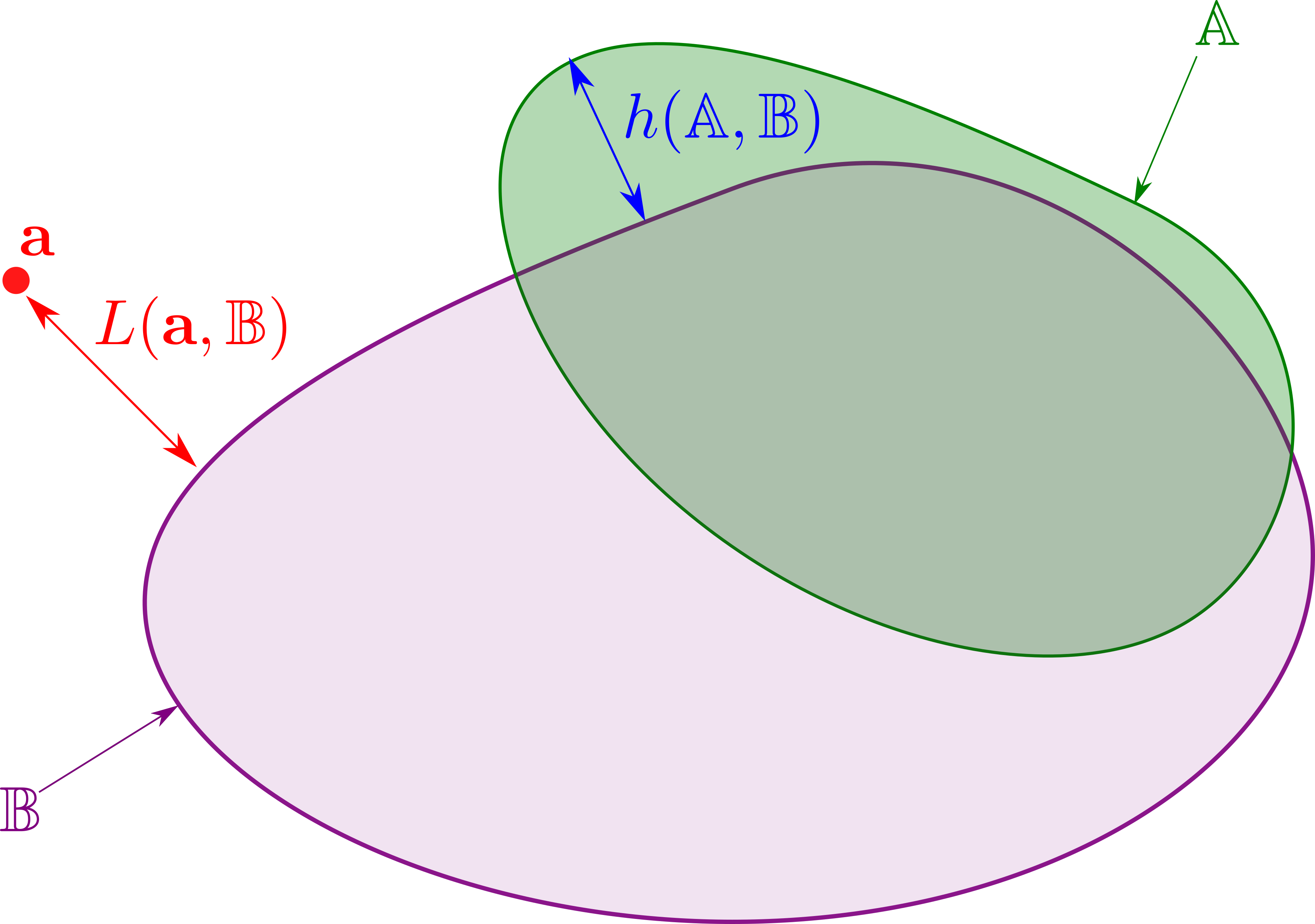
Figure 1: Proximity of $\mathbb{A}$ to $\mathbb{B}$

A nested sequence of closed subsets $\mathbb{B}(k)\subset\mathbb{R}^{n}$, $k\in\mathbb{N}$ is converging to $\mathbf{x}$ if

$$\begin{array}[]{c}\lim_{k\rightarrow\infty}h(\mathbb{B}(k),\{\mathbf{x}\})=0.\end{array}$$ (3)

2.2 Linear systems

The following proposition allows us to quantify the sensitivity of the solutions of a linear system of equations.

Definition 1.

Consider a point $\mathbf{x}$ which satisfies the linear system $\mathbf{A}\cdot\mathbf{x}=\mathbf{b}$, where $\mathbf{A}$ has independent lines. Consider a small variation $d\mathbf{A}$ of $\mathbf{A}$. The quantity

$$d\mathbf{x}=-\mathbf{A}^{\dagger}\cdot(d\mathbf{A}\cdot\mathbf{x}+d\mathbf{A}\cdot d\mathbf{x})$$ (4)

where

$$\mathbf{A}^{\dagger}=\mathbf{A}^{\text{T}}(\mathbf{A}\cdot\mathbf{A}^{\text{T}})^{-1}$$ (5)

is the generalized inverse of $\mathbf{A}$, satisfies

$$(\mathbf{A}+d\mathbf{A})\cdot(\mathbf{x}+d\mathbf{x})=\mathbf{b}.$$ (6)

This proposition tells us that if we move $\mathbf{A}$ a little, then, the solution set for the linear equation moves a little also, at order 1.

Proof. We have

$$\begin{array}[]{ccl}&&(\mathbf{A}+d\mathbf{A})\cdot(\mathbf{x}+d\mathbf{x})=\mathbf{b}\\ \Leftrightarrow&&\mathbf{A}\cdot\mathbf{x}+\mathbf{A}\cdot d\mathbf{x}+d\mathbf{A}\cdot\mathbf{x}+d\mathbf{A}\cdot d\mathbf{x}=\mathbf{b}\end{array}$$ (7)

Thus

$$\mathbf{A}\cdot d\mathbf{x}+d\mathbf{A}\cdot\mathbf{x}+d\mathbf{A}\cdot d\mathbf{x}=\mathbf{0}$$ (8)

i.e.

$$\mathbf{A}\cdot d\mathbf{x}=-d\mathbf{A}\cdot\mathbf{x}-d\mathbf{A}\cdot d\mathbf{x}$$ (9)

Since $\mathbf{A}$ has independent lines, the solution which minimizes $\|d\mathbf{x}\|$ is

$$d\mathbf{x}=\mathbf{A}^{\dagger}\cdot(-d\mathbf{A}\cdot\mathbf{x}-d\mathbf{A}\cdot d\mathbf{x}).\blacksquare$$ (10)

Corollary 1.

Consider the hyperplane

$$\mathcal{P}=\{\mathbf{x}\in\mathbb{R}^{n}|\mathbf{A}\cdot\mathbf{x}=\mathbf{0}\},$$ (11)

where $\mathbf{A}$ has independent lines. Consider a small variation $d\mathbf{A}$ of $\mathbf{A}$ with $\|d\mathbf{A}\|=O(\varepsilon)$ where $\varepsilon$ is small. Take a point $d\mathbf{x}\in\mathcal{P}$ with $\|d\mathbf{x}\|=O(\varepsilon)$. The distance from $d\mathbf{x}$ to $\mathcal{\tilde{P}}=\{\mathbf{x}\in\mathbb{R}^{n}|(\mathbf{A}+d\mathbf{A})\cdot\mathbf{x}=\mathbf{0}\}$ is $o(\varepsilon)$, i.e., $O(\varepsilon^{2})$.

Proof. Denote by $\hat{\mathbf{p}}$ the projection of a point $\mathbf{p}\in\mathcal{P}$ on $\mathcal{\tilde{P}}$. From (6), we have

$$\|\hat{\mathbf{p}}-\mathbf{p}\|=\|\mathbf{A}^{\dagger}\cdot d\mathbf{A}\cdot\mathbf{p}\|+o(\varepsilon).$$ (12)

If we take $\mathbf{p}=d\mathbf{x}$. We get

$$\begin{array}[]{ccl}\|d\hat{\mathbf{x}}-d\mathbf{x}\|&=&\|\mathbf{A}^{\dagger}\cdot d\mathbf{A}\cdot d\mathbf{x}\|+o(\varepsilon)\\ &=&o(\varepsilon)=O(\varepsilon^{2}).\blacksquare\end{array}$$ (13)

3 Wrappers

The approximation of sets using boxes computed using interval analysis generates a strong wrapping effect. It has been shown by several authors that it was possible to get a linear approximation with a better accuracy using other types of sets such as zonotopes [7] [8], ellipsoids [32], or doubleton [17]. Before defining the notion of wrapper to quantify the order of approximation we can get, we first recall what is a contractor.

Definition 1.

Denote by $\mathbb{IR}^{n}$ the set of boxes of $\mathbb{R}^{n}$. A contractor associated to the closed set $\mathbb{X}\subset\mathbb{R}^{n}$ is a function $\mathcal{C}:\mathbb{IR}^{n}\mapsto\mathbb{IR}^{n}$ such that

$$\begin{array}[]{ccc}\mathcal{C}([\mathbf{x}])\subset[\mathbf{x}]&&\text{(contraction)}\\ {}[\mathbf{x}]\cap\mathbb{X}\subset\mathcal{C}([\mathbf{x}])&&\text{(consistency)}\end{array}$$

The contractor $\mathcal{C}$ for $\mathbb{X}$ is minimal if $\mathcal{C}([\mathbf{x}])=\llbracket[\mathbf{x}]\cap\mathbb{X}\rrbracket$ where $\llbracket\mathbb{A}\rrbracket$ denotes the smallest box enclosing the set $\mathbb{A}$.

The following definition of a wrapper extends the concept of contractor and will be needed for convergence analysis.

Definition 2.

A wrapper associated to the closed set $\mathbb{X}\subset\mathbb{R}^{n}$ is a function $\mathcal{W}:\mathbb{IR}^{n}\mapsto\mathcal{P}(\mathbb{R}^{n})$ such that

$$\begin{array}[]{ccc}\mathcal{W}([\mathbf{x}])\subset[\mathbf{x}]&&\text{(contraction)}\\ {}[\mathbf{x}]\cap\mathbb{X}\subset\mathcal{W}([\mathbf{x}])&&\text{(consistency)}\\ \mathbf{x}\notin\mathbb{X}\Rightarrow\exists\varepsilon,\forall[\mathbf{x}]\subset B(\mathbf{x},\varepsilon),\mathcal{W}([\mathbf{x}])=\emptyset&&\text{(accuracy)}\end{array}$$

where $B(\mathbf{x},\varepsilon)$ is the box with center $\mathbf{x}$ and radius $\varepsilon$.

An illustration of a wrapper is given by Figure 2. The set $\mathbb{X}$ is a curve which could be given by an equation. For the box $[\mathbf{a}]$, the set $\mathcal{W}([\mathbf{a}])$ encloses the part of $\mathbb{X}$ which is inside $[\mathbf{a}]$. For the box $[\mathbf{b}]$, we have $\mathcal{W}([\mathbf{b}])=\emptyset$.

Figure 2: Illustration of a wrapper

The wrapper $\mathcal{W}$ for $\mathbb{X}$ has an order $1$ at point $\mathbf{x}$ if for all nested sequences of boxes $[\mathbf{x}](k)$ converging to $\mathbf{x}$, we have

$$\lim_{k\rightarrow\infty}\frac{h(\mathcal{W}([\mathbf{x}](k)),\mathbb{X})}{w([\mathbf{x}](k))}=0$$ (14)

where $w([\mathbf{x}])$ is the width of $[\mathbf{x}]$. Denote by $\text{Wrap}(\mathbb{X},\mathbf{x})$ the set of all wrappers for $\mathbb{X}$ which have an order $1$ at point $\mathbf{x}$.

The notion of order is illustrated by Figure 3. Larger is $k$, narrower is $[\mathbf{x}](k)$ and more accurate is the approximation.

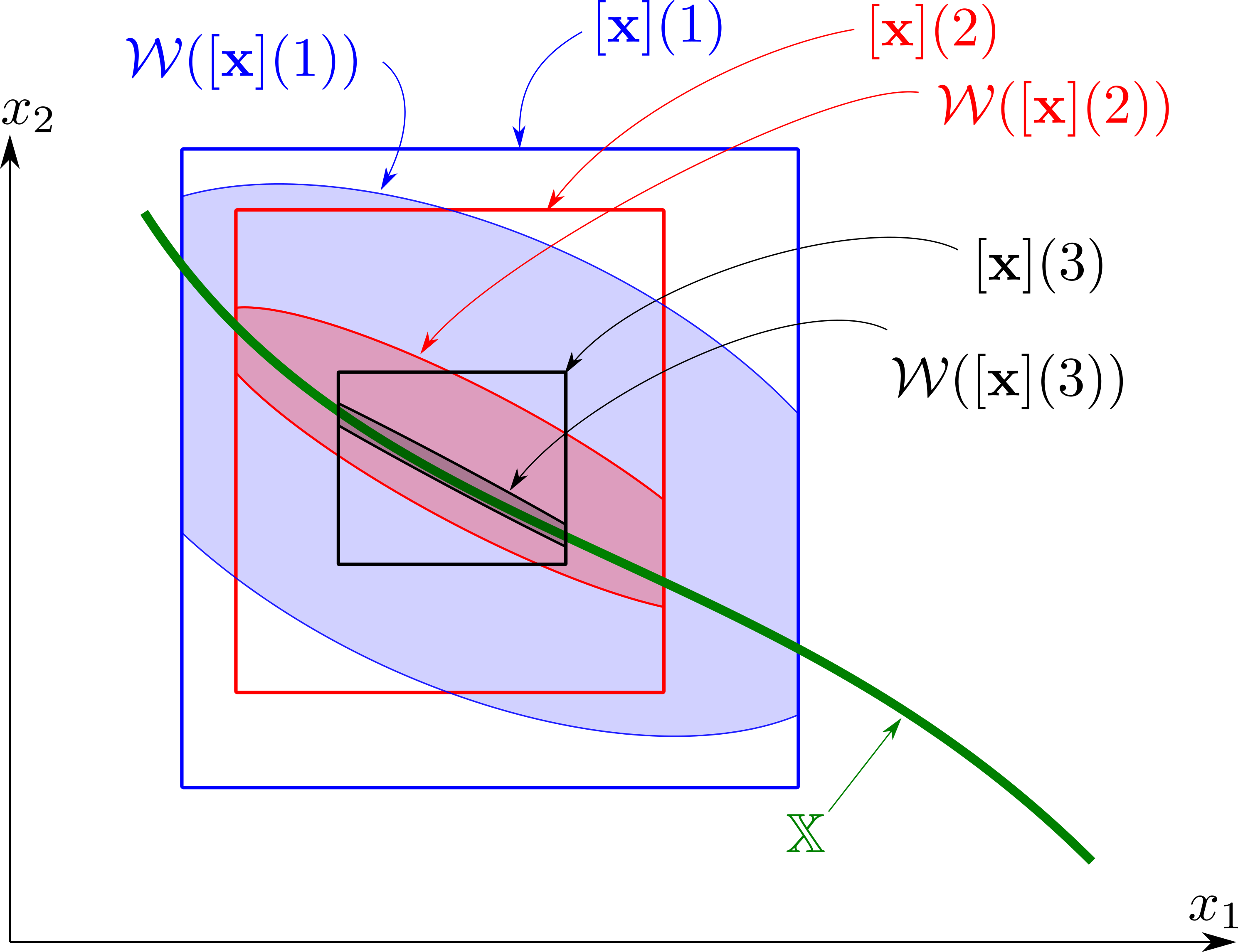
Figure 3: Wrapper of order 1

Definition 3.

We define the intersection $\mathcal{W}$ of two wrappers $\mathcal{W}_{1}$ and $\mathcal{W}_{2}$ as

$$\mathcal{W}([\mathbf{x}])=(\mathcal{W}_{1}\cap\mathcal{W}_{2})([\mathbf{x}])=\mathcal{W}_{1}([\mathbf{x}])\cap\mathcal{W}_{2}([\mathbf{x}]).$$ (15)

It is trivial to check that if $\mathcal{W}_{1}$ is a wrapper for $\mathbb{X}_{1}$ and $\mathcal{W}_{2}$ is a wrapper for $\mathbb{X}_{2}$ then $\mathcal{W}=\mathcal{W}_{1}\cap\mathcal{W}_{2}$ is a wrapper for $\mathbb{X}_{1}\cap\mathbb{X}_{2}.$ Unfortunately, the order of the approximation is not always preserved. The following proposition gives some conditions which allows us to preserve the order 1.

Definition 2.

Given $m$ sets $\mathbb{X}_{i}=\left\{\mathbf{x}\in\mathbb{R}^{n}|f_{i}(\mathbf{x})=0\right\}$, where $f_{i}:\mathbb{R}^{n}\mapsto\mathbb{R}$. Consider $\mathbb{Z}=\bigcap_{i}\mathbb{X}_{i}$ and a point $\mathbf{z}\in\mathbb{Z}.$ Assume that all $\nabla f_{i}(\mathbf{z})$ are independent. If $\mathcal{W}=\bigcap_{i}\mathcal{W}_{i}$, we have

$$\forall i,\mathcal{W}_{i}\in\text{Wrap}(\mathbb{X}_{i},\mathbf{z})\Rightarrow{\textstyle\bigcap}_{i}\mathcal{W}_{i}\in\text{Wrap}(\mathbb{Z},\mathbf{z})$$ (16)

Figure 4 illustrates that the intersection of two wrappers of order 1 at $\mathbf{z}$ is generally a wrapper of order 1 at $\mathbf{z}$. In the figure, the set $\mathbb{Z}=\mathbb{X}_{1}\cap\mathbb{X}_{2}$ is the singleton $\{\mathbf{z}\}$. The box $[\mathbf{x}]$ should be interpreted as a narrow box containing $\mathbf{z}$.

Figure 4: Intersection of two wrappers of order 1

Proof. Since $\mathbb{Z}=\bigcap_{i}\mathbb{X}_{i}$, $\mathcal{W}=\bigcap_{i}\mathcal{W}_{i}$ is a wrapper for $\mathbb{Z}$. We also need to prove that the order of $\mathcal{W}$ is 1 at $\mathbf{z}$. For this, consider a sequence $[\mathbf{x}](k)$ converging to $\mathbf{z}$. When $k$ is large $\varepsilon=w([\mathbf{x}](k))$ is small. For short, let us omit the dependency with respect to $k$. For all $\mathbf{p}\in[\mathbf{x}],$ we have $\|\mathbf{p}-\mathbf{z}\|=O(\varepsilon)$. If $\mathbb{T}_{i}$ is the tangent space of $\mathbb{X}_{i}$ at point $\mathbf{z}$ then

$$L(\mathbf{p},\mathbb{X}_{i})=L(\mathbf{p},\mathbb{T}_{i})+o(\varepsilon).$$ (17)

If all $\mathbb{T}_{i}$ are transverse, we have

$$L(\mathbf{p},\mathbb{Z})=L(\mathbf{p},{\textstyle\bigcap}_{i}\mathbb{X}_{i})=L(\mathbf{p},{\textstyle\bigcap}_{i}\mathbb{T}_{i})+o(\varepsilon).$$ (18)

Take now, $\mathbf{p}\in\mathcal{W}([\mathbf{x}])$. Since $\forall i,L(\mathbf{p},\mathbb{T}_{i})=o(\varepsilon)$ and since the $\mathbb{T}_{i}$ are transverse, we get that $L(\mathbf{p},\bigcap_{i}\mathbb{T}_{i})=o(\varepsilon)$. Therefore, from (18), $L(\mathbf{p},\mathbb{Z})=o(\varepsilon)$. Since this is true for all $\mathbf{p}\in\mathcal{W}([\mathbf{x}]),$ we have

$$h(\mathcal{W}([\mathbf{x}]),\mathbb{Z})=\sup_{\mathbf{p}\in\mathcal{W}([\mathbf{x}])}L(\mathbf{p},\mathbb{Z})=o(\varepsilon)=o(w([\mathbf{x}])).$$ (19)

Taking into account the dependency of $[\mathbf{x}]$ in $k$, we get:

$$\lim_{k\rightarrow\infty}\frac{h(\mathcal{W}([\mathbf{x}](k)),\mathbb{Z})}{w([\mathbf{x}](k))}=0.\blacksquare$$ (20)

4 Asymptotically minimal contractor

Consider the special case where wrappers, as defined by Definition 2, generate sets $\mathcal{W}([\mathbf{x}])$ that are boxes of $\mathbb{R}^{n}$. The order cannot be equal to 1 (it can only be equal to $0$), except if $n=1$. Now, we can use the wrappers of order 1, as an intermediate results, to get contractors with a good accuracy. This section defines formally such accurate contractors which is called asymptotically minimal.

Definition 4.

A contractor for $\mathbb{X}$ is asymptotically minimal at point $\mathbf{z}\in\mathbb{X}\subset\mathbb{R}^{n}$ if for any nested sequence $[\mathbf{x}](k)$ converging to $\mathbf{z}$, we have

$$\lim_{k\rightarrow\infty}\,\frac{h(\mathcal{C}([\mathbf{x}](k)),\llbracket[\mathbf{x}](k)\cap\mathbb{X}\rrbracket)}{w([\mathbf{x}](k))}=0.$$ (21)

Note that since $\mathcal{C}$ is a contractor the quantity $\mathcal{C}([\mathbf{x}](k))$ is a box.

Definition 3.

If $\mathcal{W}\in\text{Wrap}(\mathbb{X},\mathbf{z})$, then, the contractor defined by

$$\mathcal{C}([\mathbf{x}])=\llbracket\mathcal{W}([\mathbf{x}])\rrbracket$$ (22)

is an asymptotically minimal contractor for $\mathbb{X}$ at $\mathbf{z}$.

An illustration of the proposition is given by Figure 5. The gray part corresponds to the pessimism of the contractor which tends to disappear when $[\mathbf{x}]$ becomes narrow.

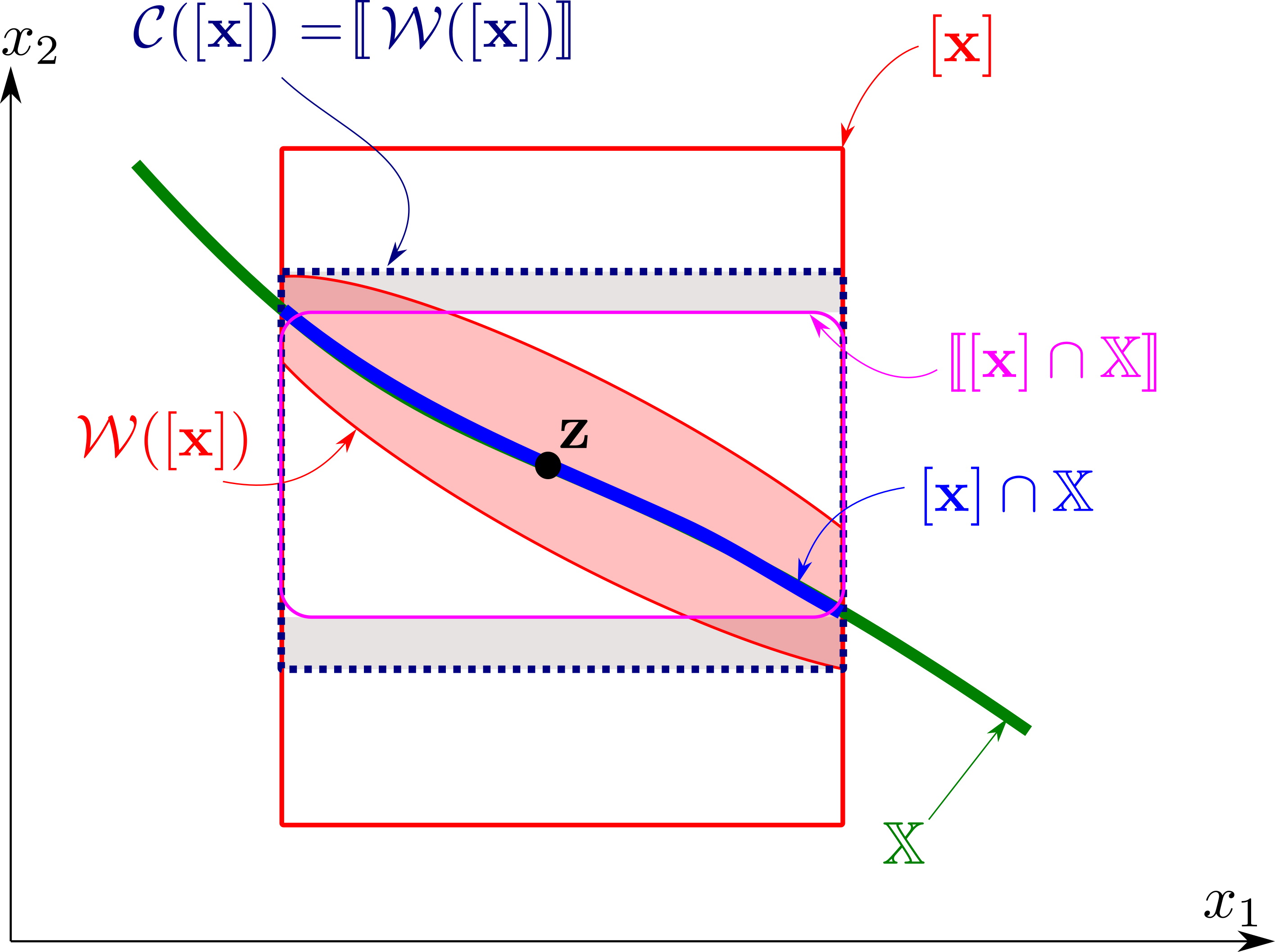
Figure 5: Asymptotic minimal contractor

Proof. The proof is by contradiction. Assume that $\mathcal{C}([\mathbf{x}])=\llbracket\mathcal{W}([\mathbf{x}])\rrbracket$ is not asymptotically minimal in $\mathbf{z}$. From (21), there exists a sequence of nested boxes such converging to $\mathbf{z}$ such that

$$\lim_{k\rightarrow\infty}\,\frac{h(\llbracket\mathcal{W}([\mathbf{x}])(k)\rrbracket,\llbracket[\mathbf{x}](k)\cap\mathbb{X}\rrbracket)}{w([\mathbf{x}](k))}>0.$$ (23)

Thus

$$\lim_{k\rightarrow\infty}\,\frac{h(\mathcal{W}([\mathbf{x}])(k),\llbracket[\mathbf{x}](k)\cap\mathbb{X}\rrbracket)}{w([\mathbf{x}](k))}>0.$$ (24)

Therefore

$$\lim_{k\rightarrow\infty}\frac{h(\mathcal{W}([\mathbf{x}](k)),\mathbb{X})}{w([\mathbf{x}](k))}>0.$$ (25)

This is inconsistent with the fact that $\mathcal{W}$ has an order 1 in $\mathbf{z}$ (see (21)).$\blacksquare$

5 Centered contractor

In this section, we show how to build an asymptotic minimal contractor using the centered form. We will consider functions $\mathbf{f}:\mathbb{R}^{n}\mapsto\mathbb{R}^{p}$ which are all continuous and differentiable. More precisely, the functions $\mathbf{f}$ are described by continuous operator of functions such as $+,-,/,\sin,\exp,\dots$ As a consequence using interval analysis, we are able to enclose the range of $\mathbf{f}$ and of $\frac{d\mathbf{f}}{d\mathbf{x}}$ over a box $[\mathbf{x}]$. In [25], Moore has proved that if $w([\mathbf{x}])=O(\varepsilon)$ then using interval computation, we get an enclosure $[\mathbf{f}]([\mathbf{x}])$ for $\mathbf{f}([\mathbf{x}])$ and an enclosure $[\frac{d\mathbf{f}}{d\mathbf{x}}]([\mathbf{x}])$ for $\frac{d\mathbf{f}}{d\mathbf{x}}([\mathbf{x}])$ such that $w([\mathbf{f}]([\mathbf{x}]))=O(\varepsilon)$ and $w(\frac{d\mathbf{f}}{d\mathbf{x}}([\mathbf{x}]))=O(\varepsilon)$.

5.1 Scalar case

Definition 4.

Consider the equation $f(\mathbf{x})=\mathbf{0}$, where $f:\mathbb{R}^{n}\mapsto\mathbb{R}$ is differentiable. The solution set is

$$\begin{array}[]{ccl}\mathbb{X}&=&\{\mathbf{x}\in\mathbb{R}^{n}\,|\,f(\mathbf{x})=\mathbf{0}\}.\end{array}$$ (26)

Consider a point $\mathbf{z}$ such that $f(\mathbf{z})=0$. Consider a nested sequence $[\mathbf{x}](k)$ converging to $\mathbf{z}$. The function $\mathcal{L}:\mathbb{IR}^{n}\mapsto\mathcal{P}(\mathbb{R}^{n})$ defined by

$$\begin{array}[]{ccl}\mathcal{L}([\mathbf{x}])&=\{&\mathbf{x}\in[\mathbf{x}]\,|\,\exists\mathbf{a}\in[\frac{df}{d\mathbf{x}}]([\mathbf{x}]),\\ &&f(\mathbf{m})+\mathbf{a}\cdot(\mathbf{x}-\mathbf{m})=0,\\ &&\mathbf{m}=\text{center}([\mathbf{x}])\}\end{array}$$ (27)

is a wrapper of order 1, i.e., it belongs to $\text{Wrap}(\mathbb{X},\mathbf{z})$. It will be called the centered wrapper associated with $f$.

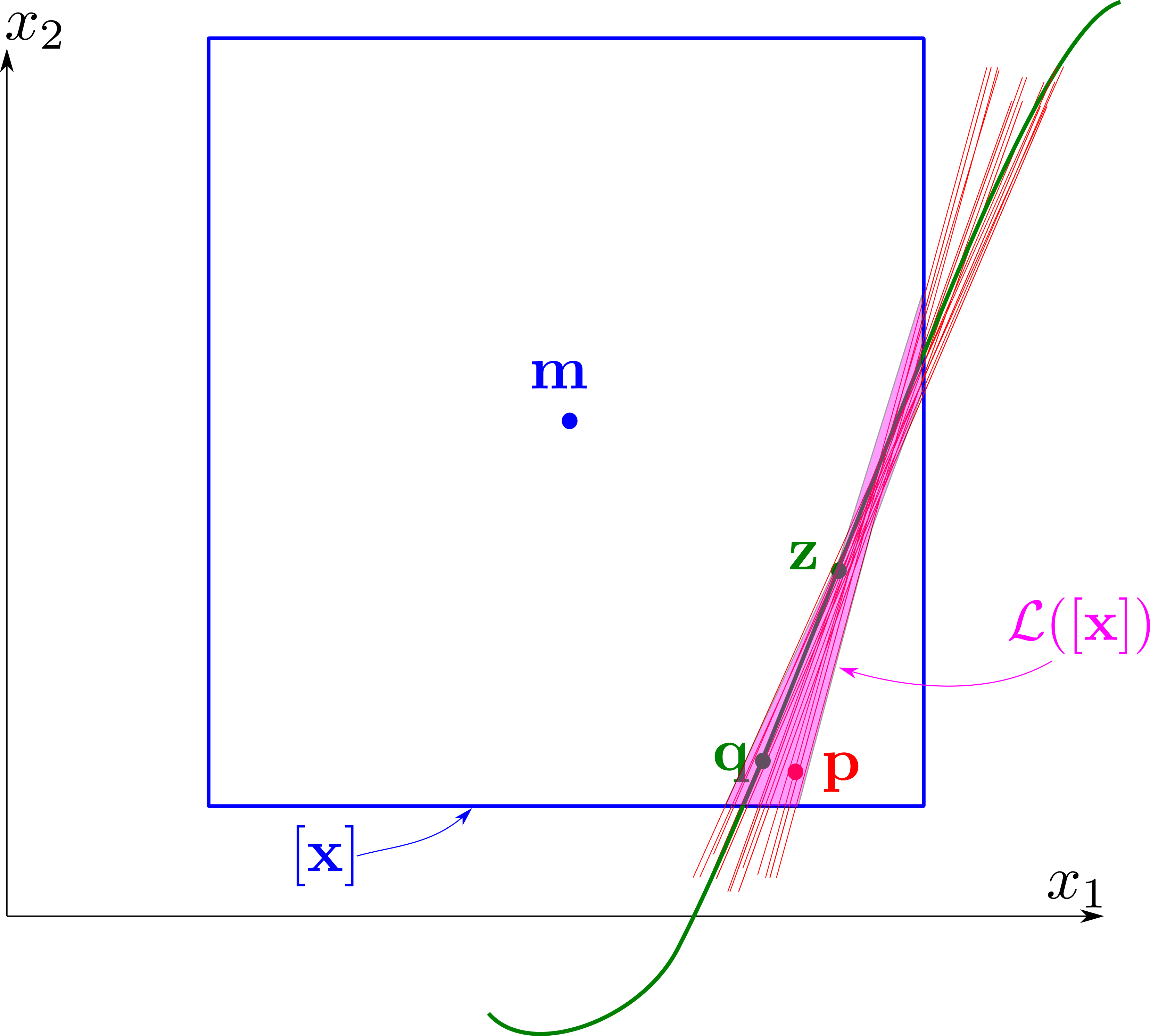
Figure 6: The set $\mathcal{L}([\mathbf{x}])$ (red) with a bowtie shape is close to the curve $\mathbb{X}$ (green)

Proof. Consider the sequence $[\mathbf{x}](k)\subset\mathbb{R}^{n}$ converging to $\mathbf{z}$. We assume that $[\mathbf{x}](k)$, or $[\mathbf{x}]$ for short, is narrow, i.e., $w([\mathbf{x}])=O(\varepsilon)$. If $\mathbf{p}\in\mathcal{L}([\mathbf{x}])$ (see Figure 6) then, for some $\mathbf{a}\in[\mathbf{a}]=[\frac{df}{d\mathbf{x}}]([\mathbf{x}])$, we have

$$f(\mathbf{m})+\mathbf{a}\cdot(\mathbf{p}-\mathbf{m})=0$$ (28)

where $\mathbf{m}=\text{center}(\text{[$\mathbf{x}$]})$. From Corollary 1, taking $d\mathbf{x}=\mathbf{p}-\mathbf{m}=O(\varepsilon)$ and since $w([\mathbf{a}])=O(\varepsilon)$, we get that the distance between a point in $\mathcal{L}([\mathbf{x}])$ and the set $\mathbb{X}$ is an $o(\varepsilon)$. We get that

$$h(\mathcal{L}([\mathbf{x}](k)),\mathbb{X})=o(w([\mathbf{x}](k)))$$ (29)

i.e.,

$$\lim_{k\rightarrow\infty}\frac{h(\mathcal{L}([\mathbf{x}](k)),\mathbb{X})}{w([\mathbf{x}](k))}=0.$$ (30)

Thus the wrapper $\mathcal{L}$ is of order 1 at $\mathbf{z}$.$\blacksquare$

Corollary 2.

The contractor for $f(\mathbf{x})=0$ defined by

$$\begin{array}[]{ccl}[x_{i}]&=&[x_{i}]\cap\left(m_{i}-f(\mathbf{m})-\sum_{j\neq i}[a_{j}]\cdot([x_{j}]-m_{j})\right)\\ {}[a_{j}]&=&[\frac{\partial f}{\partial x_{j}}]([\mathbf{x}])\end{array}$$ (31)

is asymptotically minimal.

Proof. Define $\mathcal{L}([\mathbf{x}])$ as in (27). From Proposition 3, $\mathcal{L}\in\text{Wrap}(\mathbb{X},\mathbf{z}).$ The contractor $\mathcal{C}([\mathbf{x}])=\llbracket\mathcal{L}([\mathbf{x}])\rrbracket$ is an asymptotically minimal contractor. Now the set $\mathcal{L}([\mathbf{x}])$ can be defined by the following constraints

$$\left\{\begin{array}[]{c}\exists\mathbf{z}\in[\mathbf{x}]\\ f(\mathbf{m})+\mathbf{a}\cdot(\mathbf{x}-\mathbf{m})=0\\ \mathbf{a}=\frac{\partial f}{\partial\mathbf{x}}(\mathbf{z})\\ \mathbf{m}=\text{center}([\mathbf{x}])\end{array}\right.$$ (32)

Since $\mathbf{x}$ occurs only once in the constraint $f(\mathbf{m})+\mathbf{a}\cdot(\mathbf{x}-\mathbf{m})=0$, an interval forward-backward propagation provides us the minimal contraction [24], i.e., it returns the box $\llbracket\mathcal{L}([\mathbf{x}])\rrbracket$.$\blacksquare$

5.2 Vector case

Definition 5.

Consider the equation $\mathbf{f}(\mathbf{x})=\mathbf{0}$, where $\mathbf{f}:\mathbb{R}^{n}\mapsto\mathbb{R}^{p}$ is differentiable. The solution set is

$$\begin{array}[]{ccl}\mathbb{X}&=&\{\mathbf{x}\in\mathbb{R}^{n}\,|\,\mathbf{f}(\mathbf{x})=\mathbf{0}\}.\end{array}$$ (33)

Consider a point $\mathbf{z}$ such that $\mathbf{f}(\mathbf{z})=\mathbf{0}$ and a nested sequence $[\mathbf{x}](k)$ converging to $\mathbf{z}$. Consider the wrappers $\mathcal{L}_{i}:\mathbb{IR}^{n}\mapsto\mathcal{P}(\mathbb{R}^{n})$ of order 1 for $f_{i}(\mathbf{x})=0$ defined by

$$\begin{array}[]{ccc}\mathcal{L}_{i}([\mathbf{x}])&=\{&\mathbf{x}\in[\mathbf{x}]\,|\,\exists\mathbf{a}\in[\frac{df_{i}}{d\mathbf{x}}]([\mathbf{x}]),\\ &&f_{i}(\mathbf{m})+\mathbf{a}_{i}\cdot(\mathbf{x}-\mathbf{m})=0,\\ &&\mathbf{m}=\text{center}([\mathbf{x}])\}.\end{array}$$ (34)

The operator $\bigcap_{i}\mathcal{L}_{i}$, belongs to $\text{Wrap}(\mathbb{X},\mathbf{z})$.

Proof. It is a direct consequence of Proposition 2. $\blacksquare$

To compute $\bigcap_{i}\mathcal{L}_{i}$, the method proposed for the scalar case is not valid anymore. An interval linear method could be used [28] [1]. An other possibility is to use a preconditioning method based on the Gauss-Jordan decomposition, which will be minimal in many cases, such as the test-case that will be treated in Section 6.

5.3 Preconditioning

Consider the equation $\mathbf{f}(\mathbf{x})=\mathbf{0}$, where $\mathbf{f}:\mathbb{R}^{n}\mapsto\mathbb{R}^{p}$ is differentiable. Intersecting sets $\mathcal{L}_{i}([\mathbf{x}])$ as suggested by Proposition 5 requires the resolution of interval linear equations. This operation is costly and should be avoided if it has to be repeated a large number of times. Instead of this, we prefer to use a specific preconditioning method.

To understand the principle of the preconditioning, consider the following interval linear system

$$\left(\begin{array}[]{ccc}d_{11}&d_{12}&0\\ 0&d_{22}&d_{23}\end{array}\right)\left(\begin{array}[]{c}x_{1}\\ x_{2}\\ x_{3}\end{array}\right)=\left(\begin{array}[]{c}b_{1}\\ b_{2}\end{array}\right)$$ (35)

where

$$d_{ij}\in[d_{ij}],x_{j}\in[x_{j}],b_{i}\in[b_{i}]$$ (36)

The optimal contraction can be obtained by a simple interval propagation. This is due to the fact that the corresponding constraint network as no cycle [24], as illustrated by Figure 7.

Figure 7: The constraint network has no cycle (it is a tree). Thus the interval propagation is minimal

Note that no cycle would have been obtained with the following linear system:

$$\left(\begin{array}[]{cccc}d_{11}&d_{12}&0&0\\ 0&d_{22}&d_{23}&0\\ 0&0&d_{33}&d_{34}\end{array}\right)\left(\begin{array}[]{c}x_{1}\\ x_{2}\\ x_{3}\\ x_{4}\end{array}\right)=\left(\begin{array}[]{c}b_{1}\\ b_{2}\\ b_{3}\end{array}\right)$$ (37)

A matrix $\mathbf{D}$ such that the system $\mathbf{D}\cdot\mathbf{x}=\mathbf{b}$ has no cycle can be called a tree matrix.

Both systems (35) and (37), for which the matrix $\mathbf{D}$ is a band matrix [2], could be obtained from a Gauss Jordan transformation of a linear systems [20]. For instance, if we have a system of the form $\mathbf{Ax}=\mathbf{c}$ where $\mathbf{A}$ is of dimension $3\times 4$ with full rank, there exists a matrix $\mathbf{Q}$ of dimension $3\times 3$ such that

$$\mathbf{Ax}=\mathbf{c}\Leftrightarrow\mathbf{Q}\cdot\mathbf{A\cdot}\mathbf{x}=\mathbf{Q}\cdot\mathbf{c}$$ (38)

where $\mathbf{D}=\mathbf{Q}\cdot\mathbf{A}$ has the form given by (37).

Definition 6.

Consider a set $\mathbb{X}=\left\{\mathbf{x}\in\mathbb{R}^{n}|\mathbf{f}(\mathbf{x})=\mathbf{0}\right\}$. Take a narrow box $[\mathbf{x}]$ with center $\mathbf{m}$. Assume that $\frac{d\mathbf{f}}{d\mathbf{x}}(\mathbf{m})$ is a tree matrix. An interval propagation on the system

$$\begin{array}[]{c}\mathbf{f}(\mathbf{m})+\mathbf{A}\cdot(\mathbf{x}-\mathbf{m})=\mathbf{0}\\ \mathbf{A}\in[\frac{d\mathbf{f}}{d\mathbf{x}}]([\mathbf{x}])\\ \mathbf{x}\in[\mathbf{x}]\end{array}$$ (39)

corresponds to an asymptotically minimal contractor for $\mathbb{X}.$

Proof. The interval matrix $[\mathbf{A}]=[\frac{d\mathbf{f}}{d\mathbf{x}}]([\mathbf{x}])$ is such that $w([\mathbf{A}])=O(\varepsilon)$, where $\varepsilon=w([\mathbf{x}])$. Due to the fact that the contractor $\mathcal{C}$ resulting from the interval propagation is minimal for $\mathbf{A=}\frac{d\mathbf{f}}{d\mathbf{x}}(\mathbf{m})$, and taking into account Proposition 1, we get that the contractor obtained by an elementary interval propagation is asymptotically minimal.$\blacksquare$

Corollary 3.

Consider a set $\mathbb{X}=\left\{\mathbf{x}\in\mathbb{R}^{n}|\mathbf{f}(\mathbf{x})=\mathbf{0}\right\}$. Take a narrow box $[\mathbf{x}]$ with center $\mathbf{m}$. Define $\mathbf{Q}$ such that $\mathbf{Q}\cdot\frac{d\mathbf{f}}{d\mathbf{x}}(\mathbf{m})$ is a tree matrix. An interval propagation on the system

$$\begin{array}[]{c}\mathbf{Q}\cdot\mathbf{f}(\mathbf{m})+\mathbf{Q}\cdot\mathbf{A}\cdot(\mathbf{x}-\mathbf{m})=\mathbf{0}\\ \mathbf{A}\in[\frac{d\mathbf{f}}{d\mathbf{x}}]([\mathbf{x}])\\ \mathbf{x}\in[\mathbf{x}]\end{array}$$ (40)

corresponds to an asymptotically minimal contractor for $\mathbb{X}.$

Proof. It suffices to apply Proposition 6 with $\mathbf{g}(\mathbf{x})=\mathbf{Q}\cdot\mathbf{f}(\mathbf{x})$.$\blacksquare$

5.4 Algorithm

Consider the system $\mathbf{f}(\mathbf{x})=\mathbf{0}$ and take a box $[\mathbf{x}]$. The following algorithm corresponds to a centered contractor.

Input:	f,$[\mathbf{x}]$
1	$\mathbf{m}=\text{center}([\mathbf{x}])$
2	Compute the Gauss-Jordan matrix $\mathbf{Q}$ for $\frac{d\mathbf{f}}{d\mathbf{x}}(\mathbf{m})$
3	Define $\mathbf{g}(\mathbf{x})=\mathbf{Q}\cdot\mathbf{f}(\mathbf{x})$
4	For $i\in\{1,\dots,p\}$
5	For $j\in\{1,\dots,n\}$
6	$[\mathbf{a}]=$$[\frac{\partial g_{i}}{\partial\mathbf{x}}]([\mathbf{x}])$
7	$[s]={\displaystyle\sum_{k\neq j}}[a_{k}]\cdot([x_{k}]-m_{k})$
8	$[x_{j}]=[x_{j}]\cap\left(-g_{i}(\mathbf{m})-[s]\right)$
9	Return $[\mathbf{x}]$

• Step 1 takes the center $\mathbf{m}$ of $[\mathbf{x}]$ in order to form a linear approximation for $\mathbf{f}$ in $[\mathbf{x}]$:

  $$\mathbf{f}(\mathbf{x})=\mathbf{f}(\mathbf{m})+\frac{d\mathbf{f}}{d\mathbf{x}}(\mathbf{m})\cdot(\mathbf{x}-\mathbf{m}).$$ (41)

• Step 2 returns an invertible $m\times m$ matrix $\mathbf{Q}$ such that $\mathbf{A}=\mathbf{Q}\cdot\frac{d\mathbf{f}}{d\mathbf{x}}(\mathbf{m})$ is a band matrix. The matrix $\mathbf{Q}$ is chosen by a Gauss-Jordan algorithm. The new system to be solved is now

  $$\mathbf{Q}\cdot\mathbf{f}(\mathbf{x})=\mathbf{0}.$$ (42)

• Step 3 defines $\mathbf{g}(\mathbf{x})=\mathbf{Q}\cdot\mathbf{f}(\mathbf{x}-\mathbf{m}).$ We need to solve $\mathbf{g}(\mathbf{x})=\mathbf{0}$ in the box $[\mathbf{x}]-\mathbf{m}$. The main difference compared to the previous system $\mathbf{f}(\mathbf{x})=\mathbf{0}$ is that its linear approximation

  $$\mathbf{g}(\mathbf{x})=\mathbf{g}(\mathbf{m})+\mathbf{A}\cdot(\mathbf{x}-\mathbf{m}).$$ (43)

  is such that $\mathbf{A}$ is a band matrix.

• Step 4-9 define the set of constraints

  $$\left\{\begin{array}[]{c}\mathbf{0}=\mathbf{g}(\mathbf{m})+\mathbf{A}\cdot(\mathbf{x}-\mathbf{m})\\ \mathbf{A}\in[\frac{d\mathbf{g}}{d\mathbf{x}}]([\mathbf{x}])\\ \mathbf{x}\in[\mathbf{x}]\end{array}\right.$$ (44)

  and performs an interval propagation. Due to the fact that the system has no cycle (at first order) then the propagation is asymptotically minimal.

6 Test case

Interval methods have been shown to be very powerful for the stability analysis of linear systems [21]. We have chosen to consider the linear time-delay system [35] given by

$$\ddot{x}+2\dot{x}(t-p_{1})+x(t-p_{2})=0$$ (45)

but other types of linear systems [23] with fractional orders could be considered as well. Its characteristic function is

$$\theta(\mathbf{p},s)=s^{2}+2se^{-sp_{1}}+e^{-sp_{2}}.$$ (46)

For a given $\mathbf{p}$, the location of the roots for $\theta(\mathbf{p},s)$ provides an information concerning the stability of the system. For instance, if all roots are on the half left of the complex plane, then the system is stable. The stability changes when one root crosses the imaginary line. This is the reason why we are interested in characterizing the set

$$\mathcal{P}=\{\mathbf{p}\,|\,\exists\omega>0,\,\theta(\mathbf{p},j\omega)=0\}.$$ (47)

Now

$$\begin{array}[]{cl}&\theta(p_{1},p_{2},j\omega)\\ =&-\omega^{2}+2j\omega e^{-j\omega p_{1}}+e^{-j\omega p_{2}}\\ =&-\omega^{2}+2j\omega(\cos(\omega p_{1})-j\sin(\omega p_{1}))\\ &+\cos(\omega p_{2})-j\sin(-\omega p_{2})\\ =&-\omega^{2}+2\omega\sin(\omega p_{1})+\cos(\omega p_{2})\\ &+j\cdot\left(2\omega\cos(\omega p_{1})-\sin(\omega p_{2})\right)\end{array}$$ (48)

We have

$$\begin{array}[]{cl}&\theta(p_{1},p_{2},j\omega)=0\\ \Leftrightarrow&\underset{\mathbf{f}(p_{1},p_{2},\omega)}{\underbrace{\left(\begin{array}[]{c}-\omega^{2}+2\omega\sin(\omega p_{1})+\cos(\omega p_{2})\\ 2\omega\cos(\omega p_{1})-\sin(\omega p_{2})\end{array}\right)}}=0\end{array}$$ (49)

Take $[p_{1}]=[0,2.5]$, $[p_{2}]=[1,4]$,$[\omega]=[0,10]$ and let us characterize the set $\mathcal{P}$ using the centered contractor. Using a branch and prune algorithm with a accuracy of $\varepsilon=2^{-8}$ with an HC4 algorithm [5][3] (the state of the art), we get the paving of Figure 8 in 4 sec. The number of boxes of the approximation is $43173.$ Similar results where obtained were obtained on the same example in [22].

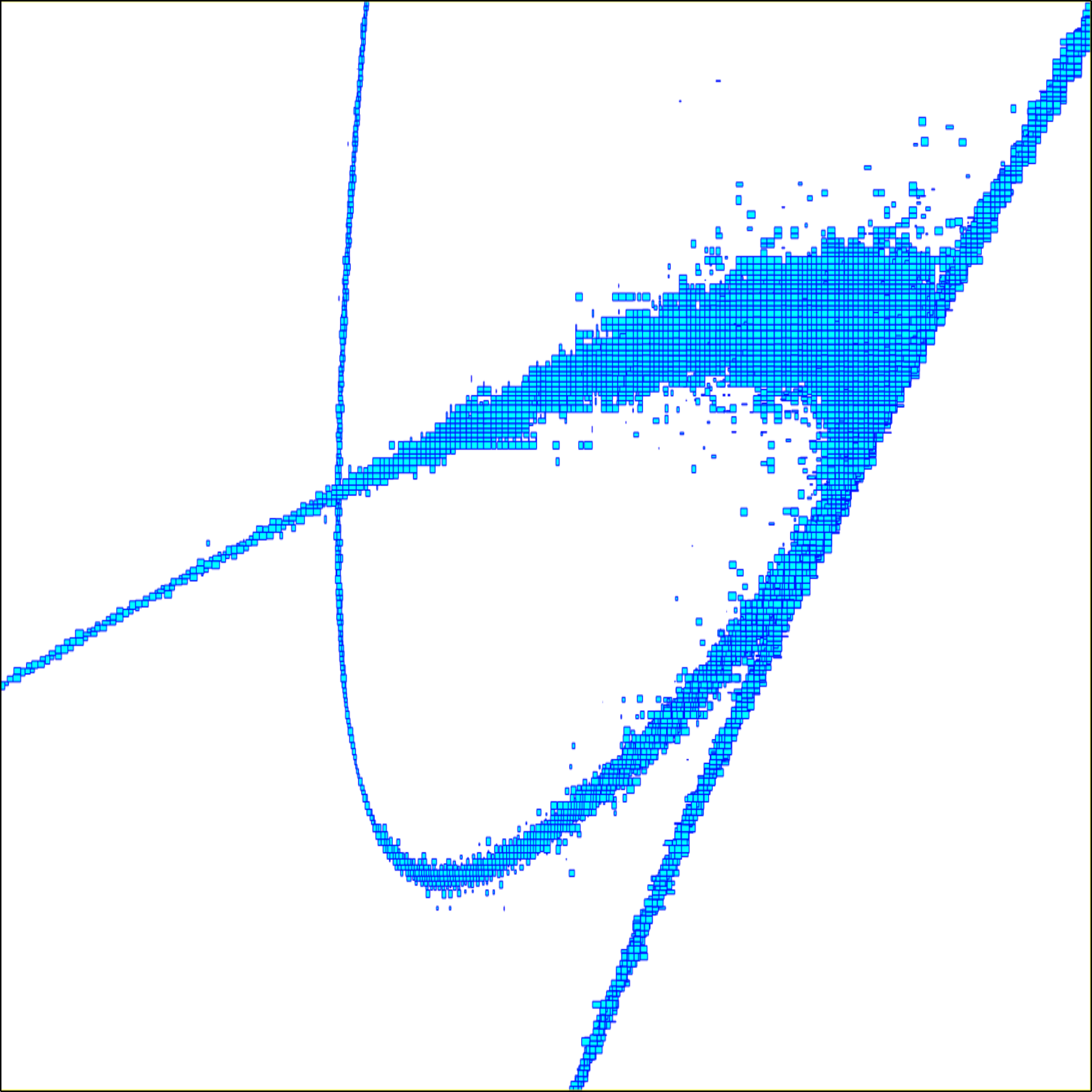
Figure 8: Approximation of the solution set with a state of the art contractor. The frame box for $(p_{1},p_{2})$ is $[0,2.5]\times[2,4]$

With an accuracy of $\varepsilon=2^{-4}$ with the centered contractor given in Section 5.4, we get the paving of Figure 9 in 1.2 sec. The number of boxes of the approximation is 282 (instead of 43173), for a more accurate approximation.

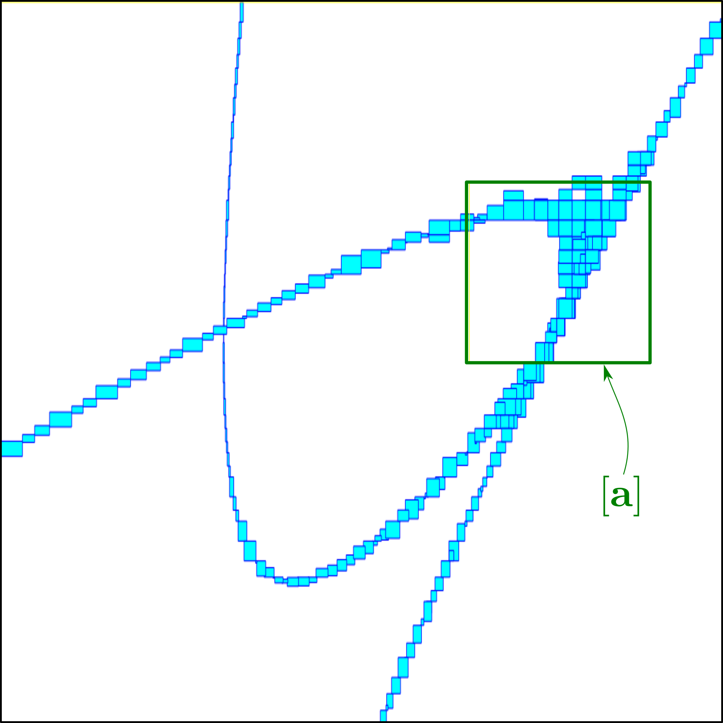
Figure 9: Paving obtained with the centered contractor. The frame box for $(p_{1},p_{2})$ is $[0,2.5]\times[2,4]$

With a accuracy of $\varepsilon=2^{-8}$ with the centered contractor, we get the thin curve represented on Figure 10. This curve is made with the small boxes generated by the paver, which shows the quality of the approximation. The big blue boxes are those already painted in the green box $[\mathbf{a}]$ of Figure 9.

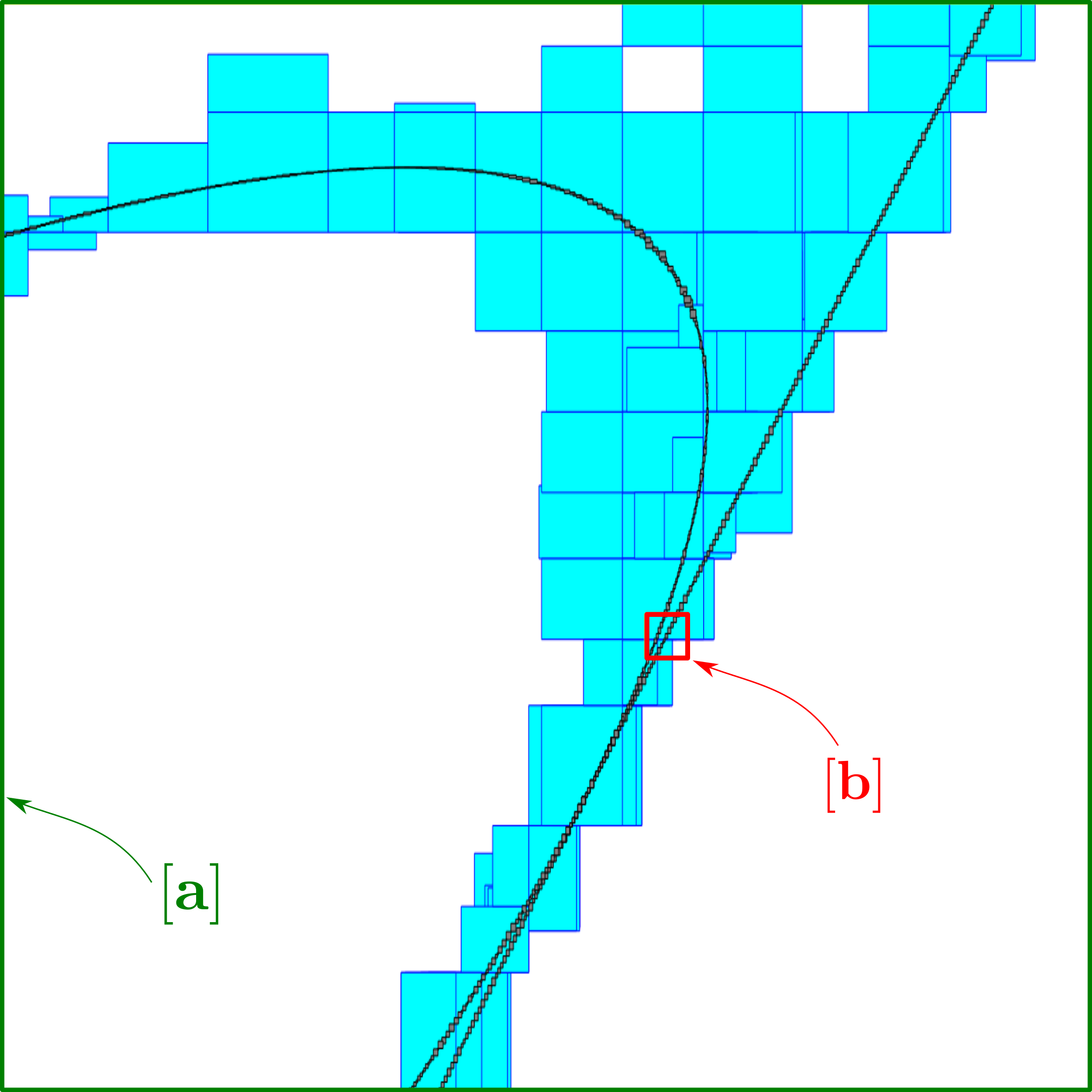
Figure 10: Pavings obtained with the centered contractor in the box $[\mathbf{a}]=[1.3,1.8]\times[3.0,3.5]$; Blue: $\varepsilon=2^{-4}$ ; Thin: $\varepsilon=2^{-8}$

With a accuracy of $\varepsilon=2^{-12}$ with the centered contractor, we get the magenta curve of Figure 11. The big gray boxes are those already painted in the red box $[\mathbf{b}]$ of Figure 10. The fact that, for a small $\varepsilon$ , the boxes of the approximation only overlap on their corners illustrates the minimality of the contractor.

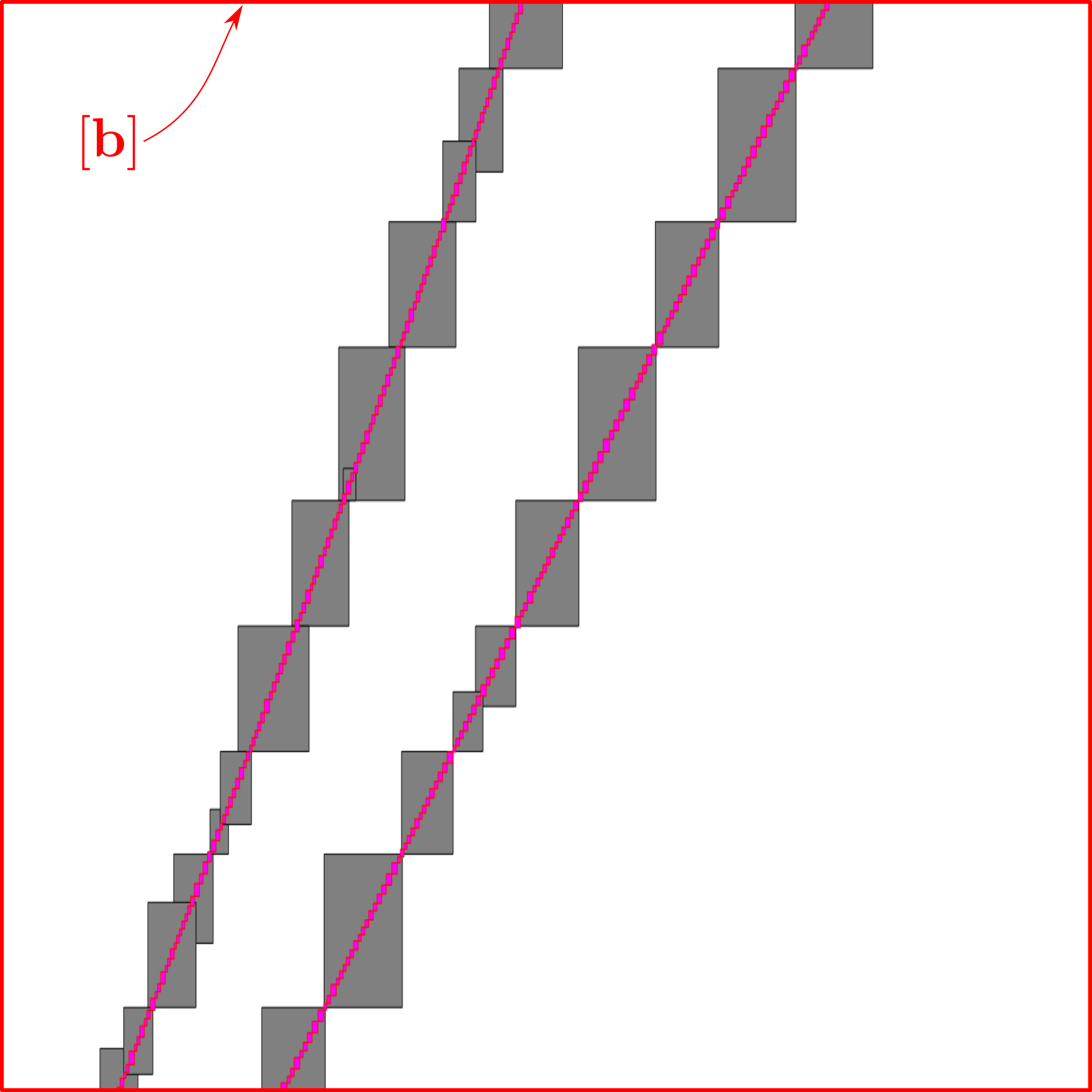
Figure 11: Approximation of the solution set in $[\mathbf{b}]=[1.595,1.615]\times[3.2,3.22]$; Gray: $\varepsilon=2^{-8}$ ; Magenta: $\varepsilon=2^{-12}$

The computing time to get the three Figures 9, 10 and 11 is less than 10 sec. Our results are much more accurate than those obtained in Section 6 of [22].

The code and an illustrating video are given at
www.ensta-bretagne.fr/jaulin/centered.html

7 Conclusion

In this paper, we have proposed a contractor which is asymptotically minimal for the approximation of a curve defined by nonlinear equations. The resulting centered contractor is based on the centered form which suppresses the pessimism when the boxes are narrow and when we have a single equation. When we combine several equations, a preconditioning method has been proposed in order to linearize the problem into a system where a tree matrix in involved. The preconditioning has been implemented using a Gauss Jordan band diagonalization method. On an example, we have shown that our centered contractor was able to outperform the state of the art contractor based on a forward-backward propagation.

Other approaches, such as the generalized interval arithmetic [14], the affine arithmetic [11] allows to get first order approximation of the constraints. As for our paper, these arithmetics can obviously model the affine dependencies between quantities with an error that shrinks quadratically with the size of the input intervals. Now, this linear approximation is only valid when we have a single constraint and can thus not be used to build asymptotically minimal contractors without some improvements. Our approach

• does not require the implementation of a new arithmetic; it only uses the standard interval arithmetic

• generates a contractor that can be combined with other existing contractors enforcing the efficiency of the resolution.

References

- [1] I. Araya, G. Trombettoni, and B. Neveu. A Contractor Based on Convex Interval Taylor. In Proc. of CPAIOR, pages 1–16, LNCS 7298, Springer, 2012.
- [2] K. Atkinson. An Introduction to Numerical Analysis (2th ed.). John Wiley, 1989.
- [3] F. Benhamou, F. Goualard, L. Granvilliers, and J. F. Puget. Revising hull and box consistency. In Proceedings of the International Conference on Logic Programming, pages 230–244, Las Cruces, NM, 1999.
- [4] I. Braems, L. Jaulin, M. Kieffer, and E. Walter. Scientific Computing, Validated Numerics, Interval Methods, Proceedings of SCAN 2000, chapter Set Computation, computation of Volumes and Data Safety, pages 267–280. Kluwer Academic Publishers, 2001.
- [5] M. Cébério and L. Granvilliers. Solving nonlinear systems by constraint inversion and interval arithmetic. In Artificial Intelligence and Symbolic Computation, volume 1930, pages 127–141, LNCS 5202, 2001.
- [6] G. Chabert and L. Jaulin. Contractor Programming. Artificial Intelligence, 173:1079–1100, 2009.
- [7] C. Combastel. Zonotopes and kalman observers: Gain optimality under distinct uncertainty paradigms and robust convergence. Autom., 55:265–273, 2015.
- [8] C. Combastel. Functional sets with typed symbols: Mixed zonotopes and polynotopes for hybrid nonlinear reachability and filtering. Autom., 143:110457, 2022.
- [9] D. Daney, N. Andreff, G. Chabert, and Y. Papegay. Interval Method for Calibration of Parallel Robots: Vision-based Experiments. Mechanism and Machine Theory, Elsevier, 41:926–944, 2006.
- [10] A. Ehambram, R. Voges, and B. Wagner. Stereo-visual-lidar sensor fusion using set-membership methods. In 17th IEEE International Conference on Automation Science and Engineering, CASE 2021, Lyon, France, August 23-27, 2021, pages 1132–1139. IEEE, 2021.
- [11] L.H. De Figueiredo and J. Stolfi. Affine arithmetic: concepts and applications. Numerical Algorithms, 37(1):147–158, 2004.
- [12] E. Goubault and S. Putot. Robust under-approximations and application to reachability of non-linear control systems with disturbances. IEEE Control. Syst. Lett., 4(4):928–933, 2020.
- [13] R. Guyonneau, S. Lagrange, and L. Hardouin. A visibility information for multi-robot localization. In IEEE/RSJ International Conference on Intelligent Robots and Systems (IROS), 2013.
- [14] E. R. Hansen. A generalized interval arithmetic. In K. Nickel, editor, Interval Mathematics 1975, pages 7–18. Springer-Verlag, 1975.
- [15] E. R. Hansen. Bounding the solution of interval linear equations. SIAM Journal on Numerical Analysis, 29(5):1493–1503, 1992.
- [16] L. Jaulin, M. Kieffer, O. Didrit, and E. Walter. Applied Interval Analysis, with Examples in Parameter and State Estimation, Robust Control and Robotics. Springer-Verlag, London, 2001.
- [17] T. Kapela, M. Mrozek, D. Wilczak, and P. Zgliczynski. CAPD: : Dynsys: A flexible C++ toolbox for rigorous numerical analysis of dynamical systems. Commun. Nonlinear Sci. Numer. Simul., 101:105578, 2021.
- [18] V. Kreinovich, A.V. Lakeyev, J. Rohn, and P.T. Kahl. Computational Complexity and Feasibility of Data Processing and Interval Computations. Springer, 1997.
- [19] M. Langerwisch and B. Wagner. Guaranteed mobile robot tracking using robust interval constraint propagation. Intelligent Robotics and Applications, Springer, 7507:354–365, 2012.
- [20] S. Leon. Linear Algebra with Applications (8th ed.). Pearson, 2009.
- [21] S. A. Malan, M. Milanese, and M. Taragna. Robust analysis and design of control systems using interval arithmetics. Automatica, 33(7):1363–1372, 1997.
- [22] R. Malti, M.T. Rapaić, and V. Turkulov. A unified framework for robust stability analysis of linear irrational systems in the parametric space. Automatica, 2022. Second version, under review (see also https://hal.archives-ouvertes.fr/hal-03646956).
- [23] A. Mayoufi, R. Malti, M. Chetoui, and M. Aoun. System identification of MISO fractional systems: Parameter and differentiation order estimation. Autom., 141:110268, 2022.
- [24] U. Montanari and F. Rossi. Constraint relaxation may be perfect. Artificial Intelligence, 48(2):143–170, 1991.
- [25] R. Moore. Methods and Applications of Interval Analysis. Society for Industrial and Applied Mathematics, jan 1979.
- [26] M. Mustafa, A. Stancu, N. Delanoue, and E. Codres. Guaranteed SLAM; An Interval Approach. Robotics and Autonomous Systems, 100:160–170, 2018.
- [27] A. Neumaier. Interval Methods for Systems of Equations. Cambridge University Press, Cambridge, UK, 1990.
- [28] A. Neumaier and O. Shcherbina. Safe bounds in linear and mixed-integer linear programming. Math. Program., 99(2):283–296, 2004.
- [29] N. Ramdani and P. Poignet. Robust dynamic experimental identification of robots with set membership uncertainty. IEEE/ASME Transactions on Mechatronics, 10(2):253–256, 2005.
- [30] A. Rauh and E. Auer. Interval approaches to reliable control of dynamical systems. In B.M. Brown, E. Kaltofen, S. Oishi, and S.M. Rump, editors, Computer-assisted proofs - tools, methods and applications, 15.11. - 20.11.2009, volume 09471 of Dagstuhl Seminar Proceedings. Schloss Dagstuhl - Leibniz-Zentrum für Informatik, Germany, 2009.
- [31] A. Rauh and E. Auer. Modeling, Design, and Simulation of Systems with Uncertainties. Springer, 2011.
- [32] A. Rauh and L. Jaulin. A computationally inexpensive algorithm for determining outer and inner enclosures of nonlinear mappings of ellipsoidal domains. International Journal of Applied Mathematics and Computer Science, 31(3), 2021.
- [33] S. Rohou, L. Jaulin, L. Mihaylova, F. Le Bars, and S. Veres. Reliable Robot Localization. Wiley, dec 2019.
- [34] R. Sainudiin. Machine Interval Experiments: Accounting for the Physical Limits on Empirical and Numerical Resolutions. LAP Academic Publishers, Köln, Germany, 2010.
- [35] V. Turkulov, M.R. Rapaić, and R. Malti. Stability analysis of time-delay systems in the parametric space. Automatica, 2022. Provisionally accepted. Third version submitted (see also https://arxiv.org/abs/2103.15629).
- [36] J. Wan. Computationally reliable approaches of contractive model predictive control for discrete-time systems. PhD dissertation, Universitat de Girona, Girona, Spain, 2007.