Mathematics and Natural Sciences Johnny Powell Physics

The Missing Baryon Problem via Cosmological Zoom-in Simulations

List of Abbreviations

AGN	Active Galactic Nucleus
AGORA	Assembling Galaxies Of Resolved Anatomy
AMR	Adaptive Mesh Refinement
CGM	Circumgalactic Medium
COS	Cosmic Origins Spectrograph
ChaNGa	Charm N-body GrAvity solver
IDE	Integrated Development Environment
IGM	Intergalactic Medium
ISM	Interstellar Medium
$\mathbf{\Lambda}$CDM	Lambda Cold Dark Matter
QSO	Quasi-Stellar Object (a.k.a. quasar)
SPH	Smoothed Particle Hydrodynamics

Contents

1. Introduction
   1. 0.1 Newton’s Laws
   2. 0.2 Gravity
   3. 0.3 Light and Matter
   4. 0.4 Spectroscopy
   5. 0.5 Dark Matter
   6. 0.6 The Cosmic Microwave Background (CMB)
   7. 0.7 Observation and Simulation
   8. 0.8 Types of simulation
2. 1 Missing Baryons and the CGM
   1. 1.1 The Missing Baryon Problem
   2. 1.2 The Circumgalactic Medium
      1. 1.2.1 What is the CGM?
      2. 1.2.2 Observing the CGM
   3. 1.3 Insight from the Simulated CGM
3. 2 Simulation Code: ChaNGa
   1. 2.1 Gravity
   2. 2.2 Newtonian Gravity and Numerical Integration
   3. 2.3 The Barnes-Hut Algorithm
   4. 2.4 Barnes-Hut Modifications
   5. 2.5 Boundary Conditions and Ewald Summation
   6. 2.6 Force Softening
   7. 2.7 Smooth Particle Hydrodynamics (SPH)
   8. 2.8 The User’s Perspective
4. 3 Visualization and Analysis Tools
   1. 3.1 Data Visualization - yt
   2. 3.2 Comparison with Observation - trident
      1. 3.2.1 Accounting for missing ions
      2. 3.2.2 Adding missing ions
      3. 3.2.3 Synthetic Spectra
5. 4 Results
6. 5 Conclusion and Future Work
7. A Determining Wavelength Range for Custom Spectra

List of Figures

1. 1 A depiction of the mutual gravitational interaction between two massive bodies $m_{1}$ and $m_{2}$ separated by a distance $r$.
2. 2 The Bohr model of the atom, with a single orbiting electron. The central nucleus is depicted as a gray circle labelled with a “plus” sign, indicating its electric charge. The first three orbits are shown and numbered, and the orbiting electron is depicted as a dark gray dot in the first orbit. This image was adapted from a similar figure that was uploaded to Wikipedia by the user JabberWock, which can be found by visiting https://en.wikipedia.org/wiki/Bohr_model.
3. 3 A depiction of emission and absorption facilitating electron transitions between the second and third orbits for an atom, according to the classical Bohr model. On the left a photon $\gamma_{a}$, depicted as a squiggly line, is absorbed by the electron in the second orbit, causing it to transition to the third orbit. On the right, a photon $\gamma_{e}$ is emitted from an electron in the third orbit as it transitions to the second orbit. In both cases, the initial and final positions of the electrons are depicted as dark gray dots, with the arrow indicating the direction of the transition. These images were adapted from a similar figure that was uploaded to Wikipedia by the user JabberWock, which can be found by visiting https://en.wikipedia.org/wiki/Bohr_model.
4. (a)
5. (b)
6. 4 A depiction of three visible light spectra. The top spectrum is continuous, with no distinct absorption or emission features. In the middle is an emission spectrum in which light is emitted at discrete wavelengths characteristic of the emitting element. At the bottom is an absorption spectrum, exhibiting dark absorption lines in an otherwise continuous spectrum at the same characteristic wavelengths as the emission spectrum. This image was borrowed from (Atomic Spectroscopy, physicsopenlab.org, https://physicsopenlab.org/2015/11/30/atomic-spectroscopy/, accessed 27 Apr. 2022).
7. 5 A rotation curve graph for the galaxy NGC 6503. This figure was borrowed from (K. Freese, International Journal of Modern Physics D 26, 1730012-223 (2017), arXiv:1701.01840). Contributions from the galaxy’s disk and gas, as well as the contribution from the dark matter halo are shown.
8. 6 A photograph of the Holmdel Horn, with which Penzias and Wilson were first able to detect the CMB. Photo credit: Bell Labs. Source: https://www.nps.gov/parkhistory/online_books/butowsky5/astro4k.htm
9. 7 CMB data from the Planck probe launched in 2009. Image courtesy of the European Space Agency https://www.esa.int/
10. 8 A visualization of the results of a cosmological simulation performed as part of the IllustrisTNG project (J. P. Naiman, et al. Monthly Notices of the Royal Astronomical Society 477, 1206 (2018).). The volume depicted is 100 kpc across, or approximately 300 million light years.
11. 1.1 An artistic depiction of the CGM and its dynamical processes taken from (J. Tumlinson, M. S. Peeples, and J. K. Werk, Ann. Rev. Astro. Astrophysics 55, 389 (2017)). The galactic disk can be found at the center, labelled by its 15 kpc radius. Gas ejection is depicted in the outflows perpendicular to the galactic plane (top and bottom of image). Recycling from previous ejection is also shown along these outflow trajectories. Diffuse gas leftover from all three processes is depicted in purple for the surrounding region.
12. 1.2 A depiction of quasar absorption spectroscopy through the CGM of a galaxy borrowed from (C. B. Hummels, B. D. Smith, and D. W. Silvia, 847, 59 (2017), arXiv:1612.03935 [astro-ph.IM]). The “swirl” in the center represents the galactic disk, the dotted circle depicts the outer limit of the CGM. The yellow diffuse dot on the left represents the quasar source, with its highly schematic emission spectrum shown below. The eye on the right represents the observer, and the observed spectrum is shown above.
13. 1.3 A phase plot of temperature vs hydrogen density for gas within $R_{\text{vir}}$ for the EAGLE simulation at redshift zero (J. Schaye, in IAU General Assembly, Vol. 29 (2015) p. 2250900). Ions are positioned on the graph according to their respective peaks in ionization fraction, and are colored according to ionization state. The range bars associated with each plotted ion give the range over which its ionization fraction is greater than half the determined maximum. The subgraph in the upper right shows the observed wavelength of absorption features with respect to lookback time and redshift. This image was taken from (J. Tumlinson, M. S. Peeples, and J. K. Werk, Ann. Rev. Astro. Astrophysics 55, 389 (2017), arXiv:1709.09180 [astro-ph.GA]).
14. 2.1 A visual representation of an Octree decomposition for four particles taken from Apple’s GameplayKit documentation website https://developer.apple.com/documentation/gameplaykit/gkOctree
15. 2.2 A 2D analogue to the Barnes-Hut Octree, known as a Quadtree. This image was borrowed from (Cos 126 programming assignment: Barnes-hut galaxy simulator, Princeton University, (2003)), which provides a very approachable description of Barnes-Hut in two dimensions.
16. 2.3 Images representing a standard k-D tree domain decomposition (left) and the spatial binary tree decomposition used by PKDGRAV (right). This image is borrowed from (J. G. Stadel, Cosmological N-body simulations and their analysis, Ph.D. thesis, University of Washington, Seattle (2001)).
17. 2.4 A depiction of a smoothing kernel being applied to a discrete set of particles. This image was uploaded to Wikipedia by the user Jlcercos and is licensed under Creative Commons. Here the circles represent the particles, $h$ the smoothing length, and the 3D curve represents the value of the smoothing kernel for all points in space.
18. 2.5 The parameter file of a ChaNGa from AGORA’s Cosmorun Paper (S. Roca-Fàbrega, et al. 917, 64 (2021), arXiv:2106.09738 [astro-ph.GA] ), opened in a text editing program.
19. 3.1 A plot of gas density projected on the $y$-$z$ plane for an AGORA Cal IV data set.
20. 3.2 A plot of gas temperature projected on the $y$-$z$ plane for the same data set and region depicted in Fig. 3.1.
21. 3.3 A “raw” spectrum produced using an Enzo dataset according to the annotated example on trident’s documentation website: https://trident.readthedocs.io/en/latest/. The ion fields considered are H, C, N, O, and Mg. Absorption features can be seen in the 1150 to 1250 Angstrom range.
22. 3.4 The same spectrum depicted in Fig. 3.3, with the addition of a quasar background and Milky Way foreground. Source: https://trident.readthedocs.io/en/latest/.
23. 3.5 A comparison between an observed quasar absorption (top) spectrum and one generated using trident (bottom) at similar redshifts ($z\sim 0.3295$). The observed spectrum was obtained using the Cosmic Origins Spectrogaph on board the Hubble space telescope, and was made publically available by (C. W. Danforth, et al. 817, 111 (2016), arXiv:1402.2655 [astro-ph.CO] ). The synthetic spectrum was produced in trident using data from an Enzo simulation (B. D. Smith, E. J. Hallman, J. M. Shull, and B. W. O’Shea, 731, 6 (2011), arXiv:1009.0261 [astro-ph.CO] ). This figure was borrowed from the trident method paper (C. B. Hummels, B. D. Smith, and D. W. Silvia, 847, 59 (2017), arXiv:1612.03935 [astro-ph.IM]).
24. 4.1 An initial synthetic quasar spectrum generated using a ChaNGa data snapshot from (S. Roca-Fàbrega, et al. 917, 64 (2021), arXiv:2106.09738 [astro-ph.GA]) with a sightline spanning the body diagonal of the cubic simulation volume. The horizontal axis represents wavelength in Angstroms.
25. 4.2 A spectrum resulting from a quasar sightline with a length of 600 kpc and an impact parameter of 30 kpc from the center of the galaxy. The horizontal axis represents wavelength in Angstroms. Only ion species of H, C, N, O, and Mg are considered during spectrum generation. Data obtained from the ChaNGa simulation published in (S. Roca-Fàbrega, et al. 917, 64 (2021), arXiv:2106.09738 [astro-ph.GA]).
26. 4.3 A spectrum resulting from a quasar sightline with a length of 600 kpc and an impact parameter of 50 kpc from the center of the galaxy. The horizontal axis represents wavelength in Angstroms. Only ion species of H, C, N, O, and Mg are considered during spectrum generation. Data obtained from the ChaNGa simulation published in (S. Roca-Fàbrega, et al. 917, 64 (2021), arXiv:2106.09738 [astro-ph.GA]).
27. 4.4 A spectrum resulting from a quasar sightline with a length of 600 kpc and an impact parameter of 100 kpc from the center of the galaxy. The horizontal axis represents wavelength in Angstroms. Only ion species of H, C, N, O, and Mg are considered during spectrum generation. Data obtained from the ChaNGa simulation published in (S. Roca-Fàbrega, et al. 917, 64 (2021), arXiv:2106.09738 [astro-ph.GA]).
28. 4.5 A spectrum resulting from a quasar sightline with a length of 600 kpc and an impact parameter of 500 kpc from the center of the galaxy. The horizontal axis represents wavelength in Angstroms. Only ion species of H, C, N, O, and Mg are considered during spectrum generation. Data obtained from the ChaNGa simulation published in (S. Roca-Fàbrega, et al. 917, 64 (2021), arXiv:2106.09738 [astro-ph.GA]).

Abstract

This thesis explores the missing baryon problem in a computational context. An overview of the problem is given, along with a discussion regarding the relevance of the Circumgalactic Medium (CMG) and cosmological Zoom-in simulations. The mechanisms underlying the N-body code ChaNGa (H. Menon, et al., Computational Astrophysics and Cosmology 2, 1 (2015), arXiv:1409.1929), as well as the data visualization and analysis tools yt (M. J. Turk, et al., 192, 9 (2011), arXiv:1011.3514) and trident (Hummels, et al., 847, 59 (2017), arXiv:1612.03935) are presented at a conceptual level. Finally, a series of synthetic quasar absorption spectra produced by using trident on a ChaNGa dataset from (S. Roca-Fàbrega, et al., 917, 64 (2021), arXiv:2106.09738) at redshift of $z\sim 4$ are shown. The low relative flux exhibited by these spectra render absorption features indistinguishable from background noise, and possible explanations for this phenomena such as high redshift are discussed. Though the resulting spectra exhibit serious obstacles for both qualitative and quantitative interpretation, they provide a “proof-of-concept” for future work, demonstrating trident’s compatibility with ChaNGa’s data format. Future prospects for using trident to analyze the CGM as simulated by ChaNGa are discussed, as well as possible extensions of this project.

Dedication

To my mother, who made all of this possible.

Introduction

This thesis explores the application of computer simulations (specifically those involving galaxies) to a particular open question in the broader field of astrophysics. Though the reader will not walk away from this text with a comprehensive understanding of astrophysics, computer simulations, or even the specific problem at hand, it is my hope that the discussion provided herein can at least help to illuminate some important concepts relating to all three, and maybe even inspire the reader to pursue the subject in a capacity that extends beyond this document.

The purpose of this chapter is to introduce a number of concepts relevant to understanding the document as a whole. Sections 0.1-0.6 are intended as a kind of “crash course” in a number of physics concepts that are relevant to understanding this thesis. Readers who are relatively unfamiliar with field will get the most value out of these sections, while those who are already well-versed may be inclined to skip them altogether. Sec. 0.7 aims to situate this project in its appropriate context relative to astrophysics as a whole. Finally, Sec. 0.8 describes common astrophysical simulation types, including Zoom-in simulations, which are of primary importance to this project.

0.1 Newton’s Laws

The first topic that warrants discussion is that of Newton’s laws, which are foundational to modern classical mechanics [1]. They are among the first concepts taught in a physics curriculum, and readers of all backgrounds have doubtlessly already encountered them in some form. While they could be taken to be assumed knowledge in the context of this thesis, they bear repeating by virtue of their relevance to the field, if only for those who are not deeply immersed in physics in their daily lives. Drawing from [1] and [2], Newton’s laws are:

1. A body at rest will remain at rest, and a body in motion will remain in motion (at constant speed), unless acted upon by an external force.

2. The net force on a body is proportional to its mass and its acceleration, which can be expressed mathematically for a set of $n$ forces as

   $$\mathbf{F}_{\text{net}}=\sum_{i=1}^{n}\mathbf{F}_{i}=m\mathbf{a}.$$ (1)

3. For every action there is an equal and opposite reaction; forces act in opposing pairs. For two bodies, this law reads

   $$\mathbf{F}_{12}=-\mathbf{F}_{21},$$ (2)

   where $\mathbf{F}_{12}$ is the force exerted on object 1 by object 2, and $\mathbf{F}_{21}$ is the force exerted on object 2 by object 1. Note that the minus sign tells us that these forces oppose one another.

In the context of this thesis, particularly with regards to simulation techniques (see Ch. 2), it is most important to understand laws 2 and 3. By providing a direct relation between the total force acting on a body and its acceleration, the second law allows us to derive the equations that are used in the calculation for gravitational motion (namely those for position and velocity, again, refer to Ch. 2).

The third law tells us that forces act in opposing pairs. The example that was used in my high school physics class was that if you go over to your bedroom wall and start pushing on it, the wall will not move because it is also “pushing back” on you with the same amount of force in the opposite direction. This is true of all forces, not just those of the bedroom-wall variety, and as was the case for the second law, it is most relevant to this document in the gravitational context.

0.2 Gravity

Gravity is one of the main forces that drives the structural evolution of the cosmos, playing a role at all levels including cosmic filaments, galaxies, and stars [2]. Naturally this means that it is also of primary importance for many astrophysical simulations. A mathematical description of the gravitational force between two massive bodies was first derived by Isaac Newton through the application of his three laws (see Sec. 0.1) to Kepler’s laws of planetary motion [2]. For two bodies with masses $m_{1}$ and $m_{2}$, this description takes the form

$$F=G\frac{m_{1}m_{2}}{r^{2}},$$ (3)

where $r$ is the distance between the two bodies and $G$ is known as the gravitational constant, with a value of roughly $6.673\times 10^{-11}$\mathrm{N}\,\mathrm{m}^{2}\,\mathrm{k}\mathrm{g}^{-2}$$ [2]. In Newtonian gravity, $G$ is understood to be a constant of nature which necessarily appears in all gravitational force calculations [2].

Figure 1: A depiction of the mutual gravitational interaction between two massive bodies $m_{1}$ and $m_{2}$ separated by a distance $r$.

Eq. 3 is referred to as Newton’s law of universal gravitation, and can be applied to all massive bodies (not just large ones) [2]. There are a few things worth noting about this equation before moving on. First, the appearance of the mass terms $m_{1}$ and $m_{2}$ in the numerator means that gravitational force is stronger when larger masses are involved. This is why we are generally much more aware of the gravitational influence of the Earth than the other objects that happen to be around us. Secondly, the $r^{2}$ term in the denominator means that gravitational force drops off drastically with distance, which is why we tend not to be too concerned about the gravitational force exerted on us by Pluto. Finally, according to Newton’s third law, Eq. 3 is really a statement about a pair of forces acting with the same strength in opposite directions. We exert the same amount of force that the Earth exerts on us, but since the Earth is so big this doesn’t affect it that much. This is why the term gravity is often interchanged with mutual gravitation, as it causes massive bodies mutually attract each other. This is shown in Fig. 1.

0.3 Light and Matter

Interactions between light and matter are a fundamental concept in this thesis, so they warrant a brief review. I should note that in this section, and throughout the document, I use the term “light” as shorthand for electromagnetic radiation, a category that includes the light that is visible to the human eye as well as other forms of radiation such as radio waves, microwaves, and x-rays [2]. Precisely what this radiation is is a concept from electromagnetism that is beyond the scope of this document, but readers with a scientific background have likely already encountered this topic before, and others probably possess a somewhat intuitive understanding of it from life in the modern world.

In modern physics, light is understood to simultaneously exhibit particle and wave-like properties [5]. For instance, light is known to come in discrete “packets” or quanta (referred to as photons), which is characteristic of a particle. At the same time, light has both an associated frequency and wavelength, which are unequivocally wave properties. This apparent paradox regarding the nature of light is known as the wave-particle duality, and as counter intuitive as it may be, it has been verified time and again by an overwhelming body of scientific work [5]. How it is that this can be the case is an incredibly deep question in physics, one which I will not get into here. Instead, I will outline how the dual nature of light helps to inform our understanding of the way it interacts with matter, which in turn will give background for understanding how observational techniques in astrophysics work.

Before exploring what the wave-particle duality tells us about how light interacts with matter, I must first talk about matter. As many readers are likely aware, matter is composed of minuscule units called atoms. Atoms consist of even smaller electrically charged particles called protons (positive charge), neutrons (neutral charge), and electrons (negative charge) [5]. A robust and physically accurate description of atomic structure falls under the purview of quantum mechanics, which lies beyond the scope of this discussion. I will focus on a simplified classical interpretation, specifically the Bohr model of the atom [5], that draws from the theory of electrodynamics [3] as well as experimental and theoretical inquiry from the early twentieth century [5]. In the interest of simplicity, I will make a number of statements throughout this discussion that are misleading with respect to the modern understanding of atomic physics. In these cases I will provide footnotes which attempt to clarify precisely which aspects of these statements are misleading, though it should be explicitly noted that these footnotes will not act as substitutes for a robust description of the modern physical theory. Readers who are interested in understanding modern atomic models and their relation to quantum mechanics might start by looking at an undergraduate chemistry text such as [7], which provides a treatment of the subject appropriate for someone with little background in physics. Readers looking for a more physics-oriented approach can refer to Ref. [5], appropriate for a second year physics undergraduate, or Ref. [6] for a more rigorous treatment at the advanced undergraduate level. I should finally note that, although the interpretation I discuss is outdated from the perspective of modern science, it serves well as a conceptual introduction to the aspects of atomic theory that are most relevant to this thesis, which is precisely the intention of this section.

At a basic level, atoms can be thought of as having two structural components: a central body known as the nucleus, which is made of protons and neutrons, and a set of electrons orbiting said central body [5]. According to the classical interpretation of the Bohr model, the orbits of these electrons are very similar to those of the planets around the Sun (i.e. gravitational orbits), since classical electrodynamics prescribes an attractive force between bodies of opposite electric charge similar to that of Newtonian gravity (Eq. 3) [3]. There is one critical difference between electron orbits and those resulting from gravitational force: whereas gravitational systems exhibit a continuous set of orbits (i.e. if one body can orbit another at a distance $r$ as well as at a distance $2r$, then it can also orbit at all distances in between), the electrons in an atom can only occupy a discrete set of orbits [5].

Each orbit has an associated energy that an electron must possess in order to occupy it, with higher energies being associated with “farther out” orbits, and vice versa [5] [7]. In order to move from one orbit to another, an electron must experience a change in energy (either negative or positive) exactly equal to the energy difference between the two orbits in question [7]. How it is that these changes in energy occur is a question that brings us back to our discussion of light.

The primary mechanism by which electrons in atoms gain or lose energy, at least in the context of this thesis, is through light. As previously mentioned, light comes in discrete quanta called photons, which also have associated wave properties of frequency and wavelength [5]. What I have not yet mentioned is that photons also carry a specific associated energy, related to frequency $\nu$, or wavelength $\lambda$ by the equation [5]

$$E=h\nu=\frac{hc}{\lambda}.$$ (4)

When an electron in an atom encounters a photon whose energy is equal to the difference in energy between the orbit it currently occupies and a higher (or “farther out”) orbit, it absorbs that photon and “jumps” to the higher orbit [7]. This process is appropriately referred to as absorption. Conversely, electrons “want” to occupy the lowest energy orbit available to them. If a lower energy orbit is available, an electron will quickly “jump down” to that orbit, emitting a photon that carries away the exact amount of energy required to make the transition [7]. This process is referred to as emission. Fig. 3 provides a visual interpretation of these processes for the classical model.

At the beginning of this section when I said that interactions between light and matter are fundamental concepts to this thesis, I was referring to precisely the phenomena of emission and absorption. These physical processes are at the heart of a particular observational technique that is of primary importance in the context of this project, which will be discussed in the following section (Sec. 0.4).

Figure 2: The Bohr model of the atom, with a single orbiting electron. The central nucleus is depicted as a gray circle labelled with a “plus” sign, indicating its electric charge. The first three orbits are shown and numbered, and the orbiting electron is depicted as a dark gray dot in the first orbit. This image was adapted from a similar figure that was uploaded to Wikipedia by the user JabberWock, which can be found by visiting https://en.wikipedia.org/wiki/Bohr_model.

(a)

(b)

Figure 3: A depiction of emission and absorption facilitating electron transitions between the second and third orbits for an atom, according to the classical Bohr model. On the left a photon $\gamma_{a}$, depicted as a squiggly line, is absorbed by the electron in the second orbit, causing it to transition to the third orbit. On the right, a photon $\gamma_{e}$ is emitted from an electron in the third orbit as it transitions to the second orbit. In both cases, the initial and final positions of the electrons are depicted as dark gray dots, with the arrow indicating the direction of the transition. These images were adapted from a similar figure that was uploaded to Wikipedia by the user JabberWock, which can be found by visiting https://en.wikipedia.org/wiki/Bohr_model.

0.4 Spectroscopy

The discussion of absorption in the previous section centered around the case of a single photon with exactly the right amount of energy hitting an electron and exciting it to a higher energy state. In reality, absorption generally occurs when a continuous spectrum of light passes through a material [2]. In this case, the light will exhibit an absorption spectrum (Fig. 4) upon passing through the material, which looks almost identical to the original continuous spectrum, but with a few dark lines corresponding to wavelengths of absorbed photons. In contrast, a material that is heated will lose energy through emission, resulting in an emission spectrum (Fig. 4) that looks dark everywhere except for at a few specific wavelengths corresponding to emitted photons [2] [7]. In the mid 1800s scientists realized that each chemical element has a distinct set of wavelengths at which emission or absorption can occur, and that elements can therefore be identified by the spectra that they produce [2]. This had profound implications for the field of astronomy; for the first time ever scientists could make empirical determinations about the chemical composition of celestial bodies, a feat that seemed unimaginable just decades prior [2].

Spectroscopy refers to the study of matter through its interactions with light [7], and it still holds a crucial role in observational astrophysics in the modern day [2] [8]. As an observational technique, spectroscopy relies on the spectroscope, a piece of equipment that takes in light from a variety of ranges on the electromagnetic spectrum (depending on the design of the equipment) and separates it by wavelength so that its intensity can be measured [2]. The resulting spectroscopic data gives light intensity with respect to wavelength, which can provide insight into a number of properties of the source or intervening material such as chemical composition (as previously mentioned) and kinematics [8]. Discussions of spectroscopy in this thesis focus primarily on absorption spectroscopy as a means of observing low-emission gas around galaxies (see Ch. 1), as it is most pertinent to the topic at hand. Spectroscopy as an observational technique is discussed further in Sec. 1.2.2, and more details regarding its relevance in the context of astrophysical simulations can be found in Sec. 3.2.

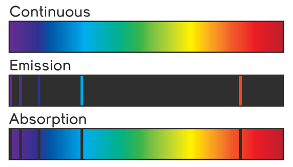
Figure 4: A depiction of three visible light spectra. The top spectrum is continuous, with no distinct absorption or emission features. In the middle is an emission spectrum in which light is emitted at discrete wavelengths characteristic of the emitting element. At the bottom is an absorption spectrum, exhibiting dark absorption lines in an otherwise continuous spectrum at the same characteristic wavelengths as the emission spectrum. This image was borrowed from (Atomic Spectroscopy, physicsopenlab.org, https://physicsopenlab.org/2015/11/30/atomic-spectroscopy/, accessed 27 Apr. 2022).

0.5 Dark Matter

Dark matter (DM) is among the oldest mysteries in physics that still remains unsolved [9]. By virtue of intrigue it is a term that is likely well-recognized by modern readers. Dark matter is used to refer to matter which cannot be detected by conventional observational means, either due to it not emitting or absorbing electromagnetic radiation (i.e. light), as would be the case for baryonic dark matter, or due to it interacting only weakly, if at all, with light [2] [11]. In more straightforward terms, DM is matter which cannot be seen using observational equipment, which relies almost exclusively on radiation originating from or passing through the material being observed.

A reasonable question arising from the fact that DM is not directly detectable is how scientists even know it exists to begin with. The answer is gravity. Specifically, advances in research into galactic rotation curves in the 1970s revealed an apparent discrepancy between the observed motion of matter in galaxies and the Newtonian prediction given the mass distribution of said matter [2] [11]. These observations showed that at greater distances from the galactic center, matter was rotating much faster than theoretical prediction indicated it should (Fig. 5) [2] [11]. This revelation led astrophysicists to postulate that a substantial fraction of the matter contained in these galaxies must exist in some unobserved form lying primarily beyond the galactic disk [2] [11]. Scientists dubbed this matter “dark matter” owing to its apparent non-interaction with light. Dark matter has since been determined to constitute the majority of the matter not only in galaxies, but in the universe as a whole [13] [2] [8].

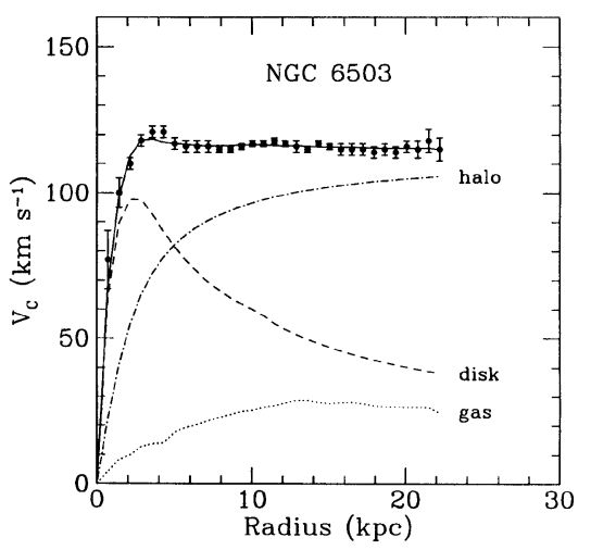
Figure 5: A rotation curve graph for the galaxy NGC 6503. This figure was borrowed from (K. Freese, International Journal of Modern Physics D 26, 1730012-223 (2017), arXiv:1701.01840 [astro-ph.CO] ) and can be found along with more information at https://ned.ipac.caltech.edu/level5/Sept17/Freese/Freese2.html. Contributions from the galaxy’s disk and gas, as well as the contribution from the dark matter halo are shown.

Understanding the nature of dark matter is a goal that is widely pursued by astrophysicists as well as scientists in adjacent fields [11], and there are undoubtedly Nobel Prizes in store for the research team that is finally able to shed light on this enigma. As exciting as the topic of dark matter is, however, unravelling a mystery which has perplexed generations of researchers would be a fairly ambitious project for an undergraduate thesis. Additionally, pragmatism dictates that research into other topics should also continue, and so it is the case that many astrophysicists pursue their work while dealing with dark matter primarily insofar as it pertains to these endeavors. This is precisely the approach adopted for this project: in light of another persistent astrophysical mystery, the missing baryon problem, we take dark matter for granted, plying our current understanding of the topic to try to understand a less widely known –but no less intriguing– cosmological conundrum. Those interested in learning more about dark matter candidates and the current state of dark matter research should look at some of the citations used in this section, namely [9] and [11].

0.6 The Cosmic Microwave Background (CMB)

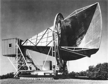
Figure 6: A photograph of the Holmdel Horn, with which Penzias and Wilson were first able to detect the CMB. Photo credit: Bell Labs. Source: https://www.nps.gov/parkhistory/online_books/butowsky5/astro4k.htm

In the early 1960s, serendipity led to a monumental discovery in observational astrophysics: the cosmic microwave background (CMB). Bell Laboratories researchers Arno Penzias and Robert Wilson were studying the Milky Way using a radio telescope that had been repurposed from a satellite antenna (see Fig. 6) [2] [14], and as they were conducting their research they noticed that their equipment was picking up a persistent background noise in the microwave range ($\sim 7.4\,$\mathrm{cm}$$) which was causing interference in their measurements [14]. This background noise appeared to be coming from all directions, and after many failed attempts at isolating its source Penzias and Wilson were at a loss. This was the case until they became aware of theoretical work that had been done around the same time by Robert Dicke and his postdoctoral student P. J. E. Peebles regarding radiation left over from the formation of the universe during the Big Bang (which at the time was still a contentious subject in theoretical astrophysics) [2]. Penzias and Wilson invited Dicke to Bell Labs, who confirmed that the instrument was, in fact, picking up the theorized cosmic microwave background [2] [14]. This discovery earned Penzias and Wilson the Nobel prize in 1978 [2]

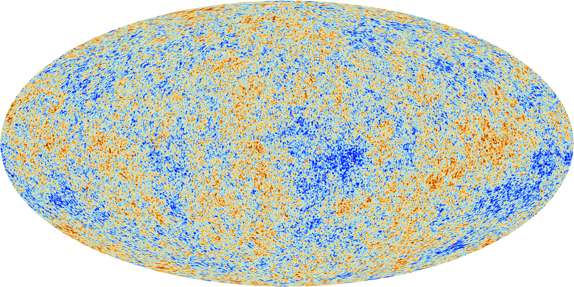
Figure 7: CMB data from the Planck probe launched in 2009. Image courtesy of the European Space Agency https://www.esa.int/

The discovery of the CMB is important for a number of reasons. Firstly, it helped to settle a crucial debate within cosmology as to whether or not the universe was steady-state (with no beginning or end). Armed with the evidence presented by the CMB, proponents of the Big Bang (the leading alternative at the time and the currently accepted theory) were able to put this debate to rest [2]. In addition to being a landmark discovery in terms of our understanding of the nature of the universe, the CMB also provides crucial insight into the state of the early universe. CMB observations pertain to this thesis in two fundamental ways. First, it is by studying the CMB that we are able to produce initial conditions for astrophysical simulations. In essence, we base simulation starting conditions on CMB observations so as to help maximize the physical realism of our results [15]. The second reason that the CMB pertains to this thesis is that CMB observations have given astrophysicists an estimate of what is known as the cosmic baryon fraction. In brief, the term baryon in astrophysics refers to any matter that interacts with light, standing in contrast to dark matter [2] [16]. Everything that you and I have ever seen in our lives has been made of baryonic matter, as is all matter that observationalists can directly detect through their telescopes. The cosmic baryon fraction, roughly speaking, tells us the fraction of baryonic matter present in the very early universe, a value which remains approximately constant over the lifetime of the cosmos [11] [8]. The importance of the cosmic baryon fraction to this thesis is discussed in greater depth in Ch. 1, but in essence it constitutes a fundamental part of the motivation behind this project.

0.7 Observation and Simulation

An important and distinctive feature of physics as a discipline is the interplay between experiment and theory. Theoretical predictions can drive experimental inquiry, and experimental findings sometimes help to shape the development of new theoretical models. Oftentimes, work in the discipline is classified in terms of its alignment within this duality, being considered either experimental or theoretical. In astrophysics, however, the distinction is not always as clear as in other sub-fields (for instance, particle physics). Experimental work, such as that which might be performed in an accelerator facility, relies heavily on laboratory environments where inquiries can be pursued in a controlled manner. Such controlled environments are essentially impossible to access for phenomena that occur at the cosmological or even galactic scale. Because of this limitation, the empirical side of astrophysics generally takes the form of observation: the detection and measurement of light incident on the Earth from astrophysical objects. There is, of course, a theoretical side to astrophysics involving the development of mathematical models for describing observed phenomena as well, and –as is the case in all areas of the field– the latter operates in concert with observation to advance our understanding of the nature of the universe.

This thesis centers heavily around computer simulations of cosmological phenomena, putting it comfortably under the umbrella of what is referred to as computational astrophysics. While there is a degree ambiguity at times in the precise placement of computational astrophysics within the experiment-theory spectrum, for the purposes of understanding this thesis, computational astrophysics should be thought about as falling firmly under the category of theory. More important than categorizations of theory versus experiment and the placement of computation therein, however, is how these concepts can help inform an understanding of the role of computation in the broader context of astrophysics.

I have already hinted at the role of computational astrophysics, but in the interest of providing context and motivation for this project it bears stating more explicitly. Broadly speaking, computer simulations help to fill in the gap left by the impossibility of performing controlled experiments at astrophysical scales. To quote Kim, et al. 2019 [17]:

“Numerical experiments are often the only means to put our theory to a test, the result of which we can compare with observational data to validate the model’s feasibility”

In essence, computer simulations offer a controlled environment through which researchers are able to probe the consequences of theoretical models for comparison against real-world observations, which can in turn help shed light on the meaning of observational results [18] (as an example, see Fig. 6 in [8] and its discussion in Sec. 4.2 of the same paper). It is thus the project of computational astrophysics, in a broad sense, to help reconcile theory with observation.

0.8 Types of simulation

The term computer simulation is a broad one. In modern science, computational techniques are applied to a broad array of problems in a variety of disciplines, and even within astrophysics computer simulations can take on many different forms. This document is specifically concerned with N-body simulations: those that model the evolution of matter under the influence of a gravitational field (as well as other physical forces, see Sec. 2.7). Such simulations start out with matter distributions that are based on early observations of the universe [15] (see Sec. 0.6) and model the dynamics of that matter so as to (ideally) produce results which exhibit structures similar to those in the real universe. For the purposes of this document, these types of simulation can be thought of as taking on one of three forms: 1.) isolated galaxy simulations, 2.) cosmological simulations, and 3.) zoom-in simulations.

Because they are arguably the simplest both conceptually and computationally, and because they served as my own introduction to computational astrophysics, I will begin with isolated galaxy simulations. Isolated galaxy simulations are precisely what the name describes: N-body simulations modelling the evolution of a single galaxy in isolation. One of the main advantages to this type of simulation is that it provides a very high level of detail for a single galaxy for a relatively low computational cost. The main drawback is that there are a great many physical processes that occur in the cosmos which are remain unaccounted for in this approach (such as accretion and ejection [8], or galactic mergers [21]). As a result, isolated galaxy simulations are most applicable to special cases where galaxies emerge via secular evolution (or evolution largely separated from the “cosmological framework”), as is often the case for barred galaxies [21].

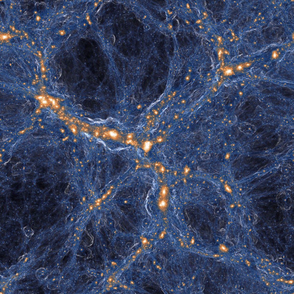
Figure 8: A visualization of the results of a cosmological simulation performed as part of the IllustrisTNG project (J. P. Naiman, et al. Monthly Notices of the Royal Astronomical Society 477, 1206 (2018).). The volume depicted is 100 kpc across, or approximately 300 million light years.

Standing in contrast to the smaller-scale approach taken by isolated galaxy simulations, cosmological simulations aim to model the large-scale structure of the universe. Fig. 8 depicts the results of one such simulation performed as part of the IllustrisTNG project [22]. The structure shown is referred to colloquially as the “cosmic web” due to its shape, observations of which were first published by Margaret Geller and John Huchra in 1989 [23]. In addition to their aesthetic beauty and the insight they provide into the shape of the universe at massive scales, such simulations also take into account crucial events that drive both galactic and cosmic evolution, such as the aforementioned mergers. The trade-off is detail. In general, cosmological simulations have lower spatial resolution than their isolated-galaxy counterparts, meaning much less data is available at the galactic scale. In essence, isolated galaxy simulations provide relatively detailed galaxies, and nothing else, while cosmological simulations provide detailed cosmological structure which is partially composed of low-detail galaxies.

The third simulation type, the Zoom-in simulation, offers a compromise between the small-scale detail of isolated galaxy simulations and the more general physical realism of cosmological simulations. The fundamental principle behind the Zoom-in method involves the identification of interesting regions within a large-scale simulation so that the program can devote more computational resources to those regions [24]. In the context of this project, this “interesting region” can simply be though of as a region which as been identified as having a galaxy of mass comparable to that the Milky Way, as this was the selection criterion for the AGORA data used in this thesis [25].

The technique used to perform Zoom-in simulations is a fairly complicated multi-step process, and I will not attempt to cover the full details here. I will, however, give a brief conceptual outline for the purpose of contextualizing the relevance of this type of simulation to the problem at hand. A Zoom-in simulation starts out as low-resolution cosmological simulation containing only dark matter (see Sec. 0.5). A gravitational simulation is then performed on that dark matter down to a redshift of zero (which can be considered “present day”), after which an algorithm known as a halo finder is used to locate galaxies within the simulation volume (the specifics of halo finding algorithms are well beyond the scope of this document, but are discussed in [24]). Once a sufficiently interesting galaxy is found, the code then restarts the simulation from the beginning, adding in baryonic matter and re-running the simulation with the identified volume-of-interest at a higher resolution [24]. As previously mentioned, the result effectively combines the strengths of isolated galaxy and cosmological simulations, providing a higher resolution “zoomed-in” region within its appropriate cosmological context. This additional level of physical realism is particularly relevant for studies involving regions such as the CGM (see Ch. 1) the evolution of which is driven by complex dynamical processes that extend well beyond the galaxy itself [8], or the IGM (e.g. [26]), which is entirely absent in isolated galaxy simulations [27]. Since this project relates to the CGM, a Zoom-in simulation is what is used to produce the data being analyzed [25].

Chapter 1 Missing Baryons and the CGM

1.1 The Missing Baryon Problem

As suggested by its title, one of the primary concerns of this thesis is a prevailing mystery in modern astrophysics that is often referred to as the missing baryon problem. This problem arises from the discrepancy between observations of the matter composition of the very early universe (specifically from the CMB, see Sec. 0.6) and the matter that is currently accounted for within galactic halos. In the vocabulary of this problem, matter can be divided into two categories: baryonic matter and dark matter. Readers who are well-versed in astrophysics lingo will likely already be familiar with the term “baryonic matter,” but for those who are not, baryonic matter constitutes all electromagnetically interacting matter, that is, any matter that interacts with light [16]. In this sense, baryonic matter is what a non-astrophysicist might refer to simply as “regular” matter, as it describes everything that can be seen (or, more accurately, observed). Readers may recall from Sec. 0.5 that the defining characteristic of the second type of matter, dark matter, is that it doesn’t interact with light (or that it only does so very weakly), putting it in contrast with baryonic matter.

Baryonic and dark matter constitute two of the fundamental “building blocks” of the universe from a cosmological perspective [2], which gives them great appeal as a line of scientific inquiry. In the early 1970s, researchers turned their attention to the newly discovered CMB as a means of understanding the matter composition of the universe [11]. Through these initial studies and decades of follow-up research, astrophysicists have been able to put increasingly precise constraints on the relative densities of baryonic and dark matter in the early universe as observed from the CMB [11]. From these measurements, we derive what is known as the cosmic baryon fraction, or the fraction of matter in the universe that is baryonic. By rough approximation (which is sufficient for understanding the problem in this context), modern measurements have the cosmic baryon fraction as being [16]

$$f_{\text{b}}\equiv\frac{\Omega_{\text{b}}}{\Omega_{\text{b}}+\Omega_{\text{d}}}\approx\frac{1}{6},$$ (1.1)

Where $\Omega_{\text{b}}$ and $\Omega_{\text{d}}$ are the measured baryonic and drak matter densities, respectively.

Measurement of the cosmic baryon fraction is what brings us to the missing baryon problem. Based on the current cosmological model, astrophysicists expect that baryonic matter is gravitationally drawn to dark matter halos, where it would eventually collapse in towards the center (i.e. the galactic disk). As a result of this process, observationalists should expect to find that the fraction of baryonic matter within the stars and Interstellar Medium (ISM) of galaxies should be close to the roughly one-sixth fraction exhibited by the cosmos [16] [8]. However, this is not observed to be the case. While quantities vary by galaxy mass, the stars and ISM account for no more than 20% of the galaxy’s expected baryon mass at best [8]. This begs the question: if so few of the baryons we expect to find are located in stars and interstellar gas, where are they? This, in essence, is the missing baryon problem. We know what the fraction of baryons to total matter is in our universe, and our theoretical model of cosmology predicts that roughly the same fraction should be present in galaxies, but our observations fall significantly short of this expectation.

There exist three possible explanations for the shortage of observed baryonic matter within galaxies. First, it is possible that the missing baryons are present in the galaxies and have simply not yet been observed. In this case, it is likely that the baryons are in a phase that is difficult to detect due to low light emission, such as cold, hot, or low-density gas [8]. Alternatively, the missing baryons could be absent from the galaxies entirely, in which case they were either accreted into the galactic halo, only to get ejected at some later point, or they failed to accrete altogether. It should be fairly clear that these are the three possibilities for the missing baryons: the baryons are in the galaxies, or they aren’t. In the latter case, they were either there at some point, or they never were to begin with. While it is important to be aware of the distinctions between these three processes, it is also important to note –as Tumlinson, et al. do in their review of modern CGM research [8]– that they are not necessarily mutually exclusive, and the true explanation for the missing baryons is most likely a combination of all three.

1.2 The Circumgalactic Medium

We have seen that there are three possible explanations for the missing baryon problem, but it may not yet be clear how this knowledge alone brings us any closer to actually finding the seemingly truant matter. What we now need is a way to observationally determine which of these explanations can account for the galactic baryon deficit. To accomplish this monumental task, astrophysicists have turned their attention to a galactic component known as the Circumgalactic Medium (CGM), which seems to hold much promise in the search for the missing baryons regardless of the cause of their absence [8].

1.2.1 What is the CGM?

As the name implies, the Circum-galactic Medium is the medium of gas and dust directly surrounding a galaxy. More precisely, while there is some ambiguity with regards to the precise boundaries of the CGM, it is generally defined as residing outside of a galaxy’s Interstellar Medium (or ISM, the gaseous medium between the stars of a galaxy) but still within its virial radius [8] [27]. The CGM is a highly dynamic region, being a site for accretion, ejection, and recycling of galactic matter [8] (see Fig. 1.1).

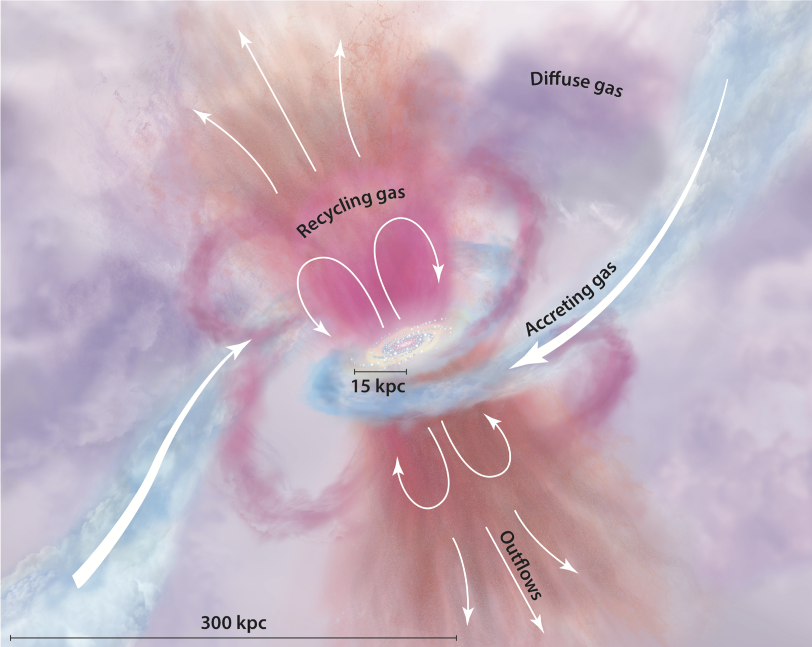
Figure 1.1: An artistic depiction of the CGM and its dynamical processes taken from (J. Tumlinson, M. S. Peeples, and J. K. Werk, Ann. Rev. Astro. Astrophysics 55, 389 (2017)). The galactic disk can be found at the center, labelled by its 15 kpc radius. Gas ejection is depicted in the outflows perpendicular to the galactic plane (top and bottom of image). Recycling from previous ejection is also shown along these outflow trajectories. Diffuse gas leftover from all three processes is depicted in purple for the surrounding region.

Already from its definition we can start to see the relevance of the CGM to the issue of the missing baryons. Being the medium that directly surrounds a galaxy’s luminous disk, the CGM acts as an interface between the galaxy’s ISM and the surrounding Intergalactic Medium (IGM) and a host for the processes that drive galaxy evolution [8] (Fig. 1.1). In essence, any matter being accreted into or ejected out of the galaxy must necessarily pass through the CGM. If we recall that one of the potential explanations for the missing baryons is ejection from galaxies, it becomes clear that on their way out, these baryons must have traversed the CGM. Because of this, we can turn to the CGM for signs of baryon ejection over the lifetime of the galaxy. More specifically, “signs of ejection” refers to heavy elements, which are produced by stellar nucleosynthesis (the fusion of lighter elements within stars), and are propagated throughout a galaxy when their parent stars go supernova [8]. The presence of these metals is significant because, along with stellar winds, supernovae are one of the main sources for the energy that causes matter to get ejected from galaxies. Therefore, observations of heavy elements (elements other than Hydrogen and Helium, also referred to as ‘metals’) in the CGM can give estimates of the energetic output of supernovae over the galaxy’s lifetime, which itself provides insight into the ejection of matter from the galaxy [16] [8].

In the case of ejection (or, conversely, failure of accretion), the significance of the CGM is perhaps most apparent. As previously noted, it is the “interface” through which matter must pass as it enters and/or leaves the galaxy, and we have seen that metals originating from stars can serve as indicators of these processes [8]. This leaves the case of the matter being present but undetected in the galaxy, for which the significance of the CGM may seem less immediately apparent. As previously stated, the most likely case for undetected baryons is that they are present in a low-emission gas phase somewhere within the galaxy. It is this precisely fact which implicates the CGM as a possible location for missing baryons. Because the CGM is composed primarily of diffuse gas, emission measurements are incredibly hard to obtain [8]. Thus, in addition to being a site for the accretion and ejection of baryonic matter, the CGM could also hold its share of unobserved baryons.

To briefly summarize, regardless of the location of the baryons or the underlying cause of their observational shortage, the CGM appears to be the best place to start looking in order to close the observational “baryon gap.” If baryons have entered the galaxy only to be ejected at a later date, we can search for signs of this ejection in the form of CGM metals. Additionally, the observational challenges associated with the CGM make it a prime location to look for undetected baryons that have not been ejected.

1.2.2 Observing the CGM

Having outlined the motivation for studying the CGM in the context of the missing baryon problem (Sec. 1.2), a discussion of how these studies are performed is now warranted. First, the challenges associated with observing the CGM bear repeating, since they are crucial to understanding the observational techniques in this context and their motivation. To reiterate from the previous section, CGM gas is partially characterized by its low density, a fact which makes observation of emission incredibly difficult [8]. Since emission studies are one of the main avenues by which observational research is performed [2], this challenge poses no small obstacle. At the same time, the observational difficulties associated with the CGM constitute a major part of the grounds on which we seek to study it in the first place, so finding a means to overcome them is important.

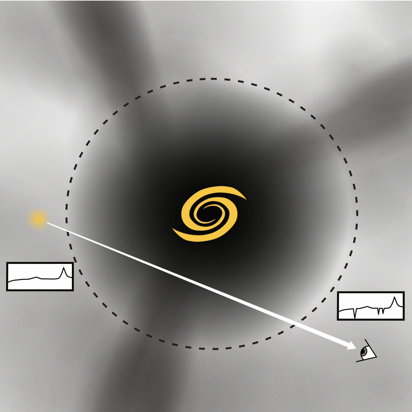
Figure 1.2: A depiction of quasar absorption spectroscopy through the CGM of a galaxy borrowed from (C. B. Hummels, B. D. Smith, and D. W. Silvia, 847, 59 (2017), arXiv:1612.03935 [astro-ph.IM]). The “swirl” in the center represents the galactic disk, the dotted circle depicts the outer limit of the CGM. The yellow diffuse dot on the left represents the quasar source, with its highly schematic emission spectrum shown below. The eye on the right represents the observer, and the observed spectrum is shown above.

There are a number of methods for collecting observational data on the CGM (see Sec. 3 of [8]). This thesis focuses in on one in particular: quasar (QSO) absorption studies (Fig. 1.2). A quasar is a type of active galactic nucleus (AGN), a dense galactic center exhibiting a significant amount of luminosity from sources other than starlight [28]. Specifically, quasars are the brightest type of AGN that are thought to be powered by supermassive black holes [29] [28]. Quasar absorption studies take advantage of the brightness of these objects by using them as background sources to perform absorption spectroscopy on intervening matter, which is particularly useful for working around the low density of CGM gas [8]. A distinct disadvantage to using quasars as background sources for CGM studies of galaxies other than our own is that we must rely on the natural occurrence of quasar sightlines passing through galaxies (we obviously cannot choose where the quasars are or what their light passes through). While this is not exceptionally uncommon, it is rare enough that in most cases only one quasar sightline is available per observed galaxy [8]. Despite having to rely on the essentially random occurrence of a quasar passing through a galaxy, the advantages offered by this method such as sensitivity to the low density of the CGM and consistency in detection irrespective of the brightness of the host galaxy [8].

1.3 Insight from the Simulated CGM

Sec. 0.7 discussed the utility of astrophysical simulations for testing theory and providing insight into observational results. As a concrete example of the latter in the context of CGM research, this subsection discusses an important figure from [8] (Fig. 1.3). This figure presents an analysis of data from the EAGLE simulation [30] which gives a log-log plot of temperature ($T$) against hydrogen density ($n_{\text{H}}$) for the gas within the simulated galaxy’s virial radius at a redshift of $z=0$ [8]. The positions of these ions on the graph represent peaks in their ionization fraction peaks with respect to $T$ and $n_{\text{H}}$ according to theoretical ionization models. To paraphrase Tumlinson, et al. [8], this graph provides a guide as to which ions are most likely to be associated with which phases of the CGM, which can help inform analysis of observational data.

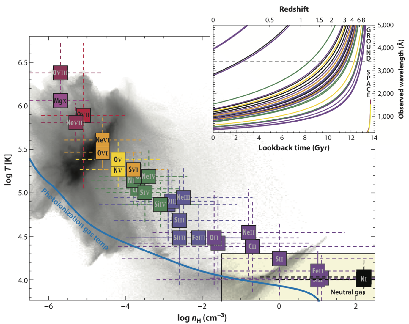
Figure 1.3: A phase plot of temperature vs hydrogen density for gas within $R_{\text{vir}}$ for the EAGLE simulation at redshift zero (J. Schaye, in IAU General Assembly, Vol. 29 (2015) p. 2250900). Ions are positioned on the graph according to their respective peaks in ionization fraction, and are colored according to ionization state. The range bars associated with each plotted ion give the range over which its ionization fraction is greater than half the determined maximum. The subgraph in the upper right shows the observed wavelength of absorption features with respect to lookback time and redshift. This image was taken from (J. Tumlinson, M. S. Peeples, and J. K. Werk, Ann. Rev. Astro. Astrophysics 55, 389 (2017), arXiv:1709.09180 [astro-ph.GA]).

This is, of course, only one example of simulations being used to give additional context to observations. Those interested in learning more should refer to Section 4 of [8], Sections 4.2 and 4.5 in particular. I should also note that this figure has little direct bearing on this project, and that my primary motivation for showing this graph is because I personally find it to be an incredibly interesting application of simulation results to observation.

Chapter 2 Simulation Code: ChaNGa

This thesis uses data from a zoom-in simulation (see Sec. 0.8) performed using an N-body code called ChaNGa (Charm N-body GrAvity solver) [31]. In this chapter I discuss a number of the techniques used by this program, as well as the motivations behind them. My hope in doing so is to provide the reader with a more robust understanding of what goes on under the hood of an N-body code, as well as a deeper appreciation for simulation codes from a technological perspective. At the same time, it is worth acknowledging that the subject matter of this chapter is very technical, and though I have not attempted to provide an exhaustive description of the code, the details that are covered can be conceptually difficult. For the reader in a hurry, an outline of the chapter is as follows: Sections 2.1-2.4 discuss gravitational motion and the code’s approach to simulating it. Sec. 2.5 describes considerations for a finite simulation of an infinite (or at least incredibly large) universe. Sec. 2.6 describes a technique for reducing gravitational force at small distances so as to avoid problems that would otherwise arise in the calculation. Sec. 2.7 describes the method by which ChaNGa accounts for the behavior of gas in the universe. Sec. 2.8 describes the process of actually using the code to get results.

2.1 Gravity

If we were to imagine ourselves sitting down at a computer, opening up our favorite IDE, and writing our own N-body code from scratch, one of the first considerations we’d need to make would be that of gravity. Gravity, after all, is precisely what makes an N-body simulation an N-body simulation! So where do we start in our treatment of gravity?

Perhaps we would like to go with a maximally accurate treatment, in which case we would be tempted to follow the gravitational model provided to us by General Relativity (GR). GR is the most widely accepted gravitational theory in modern physics, and has been studied extensively since it was first published by Albert Einstein in 1916 [32]. GR is a geometric theory which treats space and time as being fundamentally interlinked in a manifold known as spacetime. According to this theory, all gravitational motion that we observe in the three dimensional space of our universe occurs along geodesics in the spacetime manifold. The fundamental equation governing the shape of this manifold, known as Einstein’s equation, takes the form [33][10]

$$R_{\mu\nu}-\frac{1}{2}g_{\mu\nu}R=\frac{8\pi G}{c^{4}}T_{\mu\nu},$$ (2.1)

where $g_{\mu\nu}$ is a tensorial object known as the metric, which represents the curvature of the spacetime manifold (and therefore the shapes of the geodesics governing motion within said manifold), and $T_{\mu\nu}$ is known as the stress tensor or the energy-momentum tensor, which represents the mass/energy of the source generating the spacetime curvature (the phenomenon we call gravity) [33]. In essence, this equation expresses the relation between the energy/mass present in a spacetime manifold and the manifold’s shape, which itself defines the shape of gravitational trajectories. In this sense, the equation represents a means of understanding gravitational motion in the context of general relativity, hence its central role in the theory.

With all this talk of manifolds and tensors –concepts that even an advanced undergraduate is likely to be unfamiliar with– you might be getting a little concerned: how exactly are we supposed to write code that deals with such a mathematically rigorous gravitational model? The short answer is that we do not. While relativity and its implications constitute a fundamental part of the modern understanding of physics, and are certainly interesting to consider in in terms of its more philosophical implications, in all but the most extreme cases (e.g. extremely high-mass objects such as black holes), it is generally sufficient to ignore Eq. 2.1 altogether and stick with the classical treatment of gravity. Indeed, in cases of low mass and velocity, general relativity approximately reduces to Newtonian gravity, so this simplification is far from unjustified [24]. This is fortunate for us, as codes capable of treating the N-body problem relativistically do not currently exist [24]. Thus, we find that we have no choice but to engage in the time-honored physics tradition of approximation!

2.2 Newtonian Gravity and Numerical Integration

According to Newton’s law of universal gravitation (Sec. 0.2), the gravitational force between two massive particles $m_{1}$ and $m_{2}$ in 3D space is given in vector notation by the equation

$$\mathbf{F}_{1}=-\mathbf{F}_{2}=\frac{Gm_{1}m_{2}}{|\mathbf{r}_{2}-\mathbf{r}_{1}|^{3}}(\mathbf{r}_{2}-\mathbf{r}_{1}),$$ (2.2)

where $\mathbf{r}_{1}$ and $\mathbf{r}_{2}$ denote the position vectors of the two particles. Note that Eq. 2.2 is simply the vector form of the same equation expressing the magnitude of gravitational force between two bodies presented in Sec. 0.2 (Eq. 3). Of course, Eq. 2.2 is only the $N=2$ case. Noting that forces are additive (that is, $\mathbf{F}_{\text{net}}=\sum_{i}\mathbf{F}_{i}$), we can write the equation for for the gravitational force acting on the $i$th particle in a configuration of three or more massive particles as

$$\mathbf{F}_{i}=\sum_{i\neq j}\frac{Gm_{i}m_{j}}{|\mathbf{r}_{j}-\mathbf{r}_{i}|^{3}}(\mathbf{r}_{j}-\mathbf{r}_{i}).$$ (2.3)

Eq. 2.3 gives us our Newtonian approximation of gravity, so we need only solve this second order differential equation for all the particles in our simulation and it’s off to the races! Unfortunately, this equation has no analytical solution for $N>2$ [12], so rather than spending our careers trying to solve the unsolvable by determining the exact paths traced by our $N\gg 2$ particles with respect to time, we need to use a numerical integration technique to approximate these paths. A particularly common numerical method used for force integration among N-body codes [34], which also happens to be the method adopted by ChaNGa [12], is known as “leapfrog integration.” As the reader with experience in numerical methods likely already knows, the first step to making such a problem as that presented by Eq. 2.3 suitable for evaluation by a computer is discretization, the division of a continuous phenomena into appropriately small (but still finite) discrete “steps.” While the programmer has some freedom in choosing how to handle the process [12], the approach adopted in the leapfrog method is time discretization, breaking up the continuous “flow” of time into individual “chunks” (or time steps). Mathematically, the routine used for leapfrog integration (derived via Taylor expansion) is most commonly expressed using the equations [12]

$$\mathbf{v}_{n+\frac{1}{2}}=\mathbf{v}_{n-\frac{1}{2}}+\mathbf{a}_{n}\Delta t$$ (2.4)

$$\mathbf{r}_{n+1}=\mathbf{r}_{n}+\mathbf{v}_{n+\frac{1}{2}}\Delta t.$$ (2.5)

The form of Equations 2.5 and 2.4 gives a good impression of why the method is called “leapfrog” [34]: given initial values for position and velocity, first you use Eq. 2.4 to update velocity, then you use the new velocity in Eq. 2.5 to update position, and then you repeat the process alternating between velocity and position in a manner similar to the game “leapfrog”.

While Equations 2.4 and 2.5 give us the routine in a nice compact form and provide insight into its rather fun nickname, they are not the equations that ChaNGa actually uses in it’s implementation. Instead, ChaNGa uses what is known as the “kick-drift-kick” form of the routine, which can be written as [12] [15]

$$\mathbf{v}_{n+\frac{1}{2}}=\mathbf{v}_{n}+\mathbf{a}_{n}\frac{\Delta t}{2},$$ (2.6)

$$\mathbf{r}_{n+1}=\mathbf{r}_{n}+\mathbf{v}_{n+\frac{1}{2}}\Delta t,$$ (2.7)

$$\mathbf{v}_{n+1}=\mathbf{v}_{n+\frac{1}{2}}+\mathbf{a}_{n+1}\frac{\Delta t}{2}.$$ (2.8)

Taking a closer look at these equations, we can begin to see where the name “kick-drift-kick” comes from. At each step, we first update the intermediate velocity term ($\mathbf{v}_{n+\frac{1}{2}}$) using the “current” gravitational acceleration (the acceleration acting as the “kick”), then update the position ($\mathbf{r}_{n+1}$) according to this new velocity (the equation treats the particle as though it is moving in the absence of external forces, i.e. drifting), then update the velocity ($\mathbf{v}_{n+1}$) using the gravitational acceleration at the new spatial position.

There are a number of reasons why the kick-drift-kick format of the leapfrog method is favored by ChaNGa’s approach, paramount among these, however, is a concept known as multi-stepping [31]. In essence, the number of computations (Equations 2.6-2.8) made within a fixed time interval is largely what determines the physical accuracy of the algorithm. Since the method effectively amounts to an approximation in which particles move with fixed velocity between time steps, the smaller the time step, the more “true-to-life” the paths become. However, as always there is a computational tradeoff in terms of runtime, and so rather than pursuing increasingly small timesteps, the goal is generally to find a step number relative to the size of the time interval for which the path accuracy is “good enough.” Since gravity is a spatially dependent force, the notion of what constitutes a “good enough” temporal resolution is closely linked with particle density. Because of this, regions with higher particle density will naturally require smaller timesteps in order to achieve the same level of physical accuracy that can be attained in a lower density region with a larger timestep [12] [15] [35]. While one approach to this problem might be to increase the number of timesteps globally to be suitable to the desired level of accuracy in high density regions, doing so would introduce a large number of extraneous calculations for low density regions and would thus be wasteful from a computational perspective [35]. The solution to this efficiency problem is to assign time steps on a per-particle basis, that is, each particle gets its own time step size in accordance with the density of surrounding particles (multi-stepping). The kick-drift-kick method ensures that such an individualized time-step assignment is possible, so long as the time step sizes of all particles are related by powers of two [12].

2.3 The Barnes-Hut Algorithm

In the previous two sections, we discussed the use of Newtonian gravity as a weak-field approximation to the far more complicated general relativistic formulation, and the use of the leapfrog integration method to numerically evaluate motion in a Newtonian gravitational field. One might reasonably expect that this brings us close to a complete understanding of ChaNGa’s most rudimentary functionality: solving the N-body problem for purely gravitational interactions (readers who are concerned by my use of “rudimentary” here should be comforted to know that I explain myself in Sec. 2.7). Unfortunately, owing to the ever-complicated nature of the N-body problem, we find ourselves in yet another snare, that being the issue of runtime efficiency. To understand the problem, first note that the net acceleration terms in the leapfrog routine (Eq. 2.6-2.8) are actually the result of the sum of gravitational interactions expressed in Eq. 2.3. From the form of the latter, it shouldn’t be too hard to convince yourself that, in a simulation of $N$ particles, each particle experiences $N-1$ gravitational interactions. Thus, if we were to write a simulation code with just the information from Sections 2.1 and 2.2, at each time step our program would need to perform $N-1$ force calculations $N$ times which, for the reader familiar with asymptotic notation in computer science, is $O(N^{2})$ [24]. Such asymptotic behavior might be acceptable for small-scale computations, the current state of computational astrophysics is such that simulations can have particle counts well in the millions and often evolve over thousands of time steps [12] [15]. Modern codes need to accommodate for this level of scale, which necessitates methods of speeding up the gravitational force calculation process.

The solution employed by ChaNGa is to use a modified version of the Barnes-Hut algorithm [36], which offers an approximation of the gravitational force acting on a particle in logarithmic time ($O(\log N)$), making the total force calculation per timestep $O(N\log N)$, a substantial improvement from the polynomial time “direct summation” method. In the next few paragraphs, I will introduce the standard Barnes-Hut algorithm to familiarize the reader with the general approach to the problem, and will then proceed to discuss some of the modifications employed by ChaNGa and the motivations behind them. The reader searching for a more in-depth or specific treatment of Barnes-Hut might be interested in reading the original 1986 paper [36], or some of my more undergraduate-friendly sources such as [37] and [12].

The fundamental principle behind the Barnes-Hut algorithm is to reduce the number of gravitational acceleration calculations performed for each particle by applying a center-of-mass approximation for the force exerted by distant particles. More explicitly, for distant clusters –particles that are relatively far from the particle whose acceleration we want to calculate but are relatively close to each other– the algorithm determines the center of mass and total mass of the cluster, then performs a single gravitational force calculation using these values. As noted in [12], the nature of gravitation is such that for a sufficiently distant cluster of identical particles the force contribution associated with each particle will be roughly identical (both in terms of magnitude and direction), so the approximation is justified. Of course, distance constitutes the main underlying assumption for the approximation, meaning it does not hold for nearby particles, for whom direct summation is still performed.

Of course, since this approach relies so heavily on distance, we need to establish a way to determine what constitutes “far enough” for a center-of-mass approximation and “close enough” for particles to be considered part of the same cluster. On cursory inspection, one may be tempted to simply compare the distances of all the particles in the simulation, but such a process would be $O(N^{2})$ itself [12], no better than direct summation. Barnes-Hut offers a rather clever solution to this problem, which starts with a process known as “domain decomposition,” or the repeated decomposition of the initial volume into smaller subvolumes. The traditional Barnes-Hut algorithm uses an Octree decomposition structure [12] [36], in involves recursively dividing cubical volumes into eight subvolumes, hence the name. A summary of Octree decomposition is as follows:

1. Begin with the volume containing all particles, this is the “root node” of the Octree.

2. If there are no particles in the node, discard it.

3. If two or more particles are present in the cell, divide it evenly into eight “daughter nodes,” then inspect each daughter node individually.

4. repeat steps 2-3 until each node contains at most one particle.

Fig. 2.1 gives a visual example of this process for a volume containing four particles. Note the nodes vary in size according to their corresponding “level” in the tree structure. Only boxes containing more than one particle are subdivided into daughter nodes, and division is performed recursively until each node contains one or zero particles.

Figure 2.1: A visual representation of an Octree decomposition for four particles taken from Apple’s GameplayKit documentation website https://developer.apple.com/documentation/gameplaykit/gkOctree.

In total, the time complexity of constructing the Octree is $O(N\log N)$ [36], so far we are still looking at an improvement on direct summation. We still need to discuss how exactly this structure expedites the force calculation, however, an insight which may yet elude all but the most computer-savvy readers. The next step involves center of mass calculations. The implementation of the algorithm as described in the original paper [36] is such that the data structure representing a node in the tree has attributes corresponding to the total mass and center of mass (COM) for the particles contained therein. For nodes containing only one particle (dubbed “leaf nodes” in the language of the tree metaphor), these values are trivial, so it is most efficient to propagate this information backwards through the data structure, i.e. leaves-to-root, a process which is also $O(N\log N)$ [36].

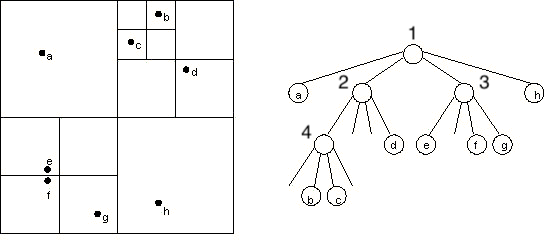
Figure 2.2: A 2D analogue to the Barnes-Hut Octree, known as a Quadtree. This image was borrowed from (Cos 126 programming assignment: Barnes-hut galaxy simulator, Princeton University, (2003)), which provides a very approachable description of Barnes-Hut in two dimensions.

If we examine the analogous 2D Quadtree data structure depicted in Fig. 2.2, we can see that the COM and total mass calculation would begin with node 4, whose corresponding attributes will be calculated using the positions and masses of particles a and b. We can then use these attributes of 4, as well as the mass and position of particle d, to compute the total mass and COM of node 2 and so on. Nodes containing more than one particle can then be treated as “pseudoparticles” with their own associated mass and position.

Once all the psuedoparticle nodes in the simulation have been assigned their mass and COM attributes, all the machinery necessary to begin force calculations is in place. The algorithm for calculating the force on a given particle $p$ involves a traversal of the Octree, where $\ell$ is the side length of the cubical region represented by the current node, $d$ is the distance between $p$ and the node’s COM, and $\theta$ is an accuracy parameter set at the start of the simulation, usually  1. With these values in mind, the algorithm for each particle goes as follows [36]

1. Start at the root node.

2. If $\ell/d<\theta$, compute the gravitational force between the current node and $p$, and add it to the total force acting on $p$.

3. Otherwise, traverse one layer down the tree and perform Step 2 for each daughter node.

4. End.

Once this algorithm has run to completion, the gravitational influence of each particle on $p$ will have been accounted for (either by direct force calculation or COM approximation), so it presents a reliable method of updating particle accelerations. For large $N$, this process involves performing order $\log N$ force calculations for each particle, so the asymptotic runtime of the algorithm is still $O(N\log N)$ overall!

2.4 Barnes-Hut Modifications

The description I’ve provided of the Barnes-Hut gravitational force computation has thus far followed closely with the original paper [36], but as previously mentioned there are a number of changes that the ChaNGa code makes to adapt the algorithm to its approach. The first notable change is that ChaNGa doesn’t actually use the center of mass of far away particle groups to approximate their gravitational influence. Instead, ChaNGa performs an operation known as a multipole expansion for improved force accuracy [31]. A sufficiently advanced physics undergraduate is likely to have encountered the multipole expansion in an E&M course (see Ch. 3.4 in [3]), where it is commonly used to model electric fields which cannot easily be calculated analytically [12]. Due to the similarities between Newtonian gravity and the electric field, this method can also be used to approximate the gravitational potential produced by analytically difficult mass distributions (e.g. clusters of massive particles).

The multipole expansion effectively amounts to an infinite sum of terms (similar to a Taylor series) with increasing angular dependence [38]. The first (or zeroth order) term is a monopole, or a point source, which has no angular dependence. The first few higher order terms are the dipole, quadrupole, and hexadecapole terms. While a derivation or a precise mathematical description of the multipole expansion are beyond the scope of this document, readers can turn to [3] or [38] for more detailed discussions in the E&M context, or to [39] for the N-body simulation context. For the reader in a hurry though, it is most important to know that ChaNGa performs a multipole expansion to third order, i.e. includes all terms up to and including hexadecapole [31], and that this is both faster and more accurate than a quadrupole order expansion [39].

A second notable difference between the 1986 Barnes-Hut algorithm and that employed by ChaNGa is the precise structure of the spatial decomposition tree. As we saw in Sec. 2.3, the algorithm as presented in the original paper recursively divides the spatial domain into even sections of eight, resulting in a data structure called an Octree (again, see Fig. 2.1). The spatial decomposition performed by ChaNGa actually employs a binary tree rather than an Octree, meaning the domain is recursively divided into sections of two rather than eight. This change is in line with the approach used by the N-body code PKDGRAV [39], from which ChaNGa inherits much of its gravitational force calculation [31]. It should be noted that the justification for using a binary tree rather than an Octree is that a binary tree structure offers advantages for code parallelization, particularly in terms of the distributing the computation over an arbitrary number of processors [39], a feature which is clearly desirable in the context of high performance computing.

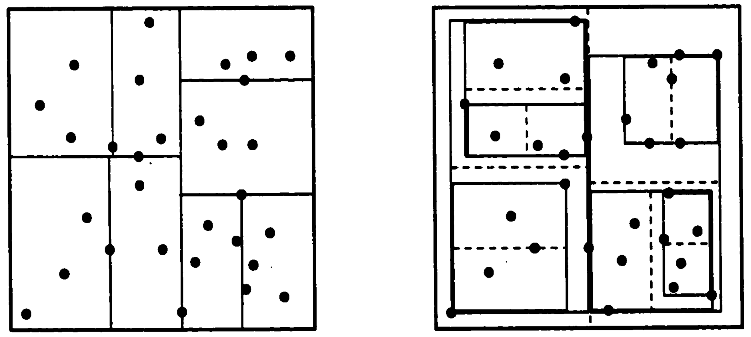
Figure 2.3: Images representing a standard k-D tree domain decomposition (left) and the spatial binary tree decomposition used by PKDGRAV (right). This image is borrowed from (J. G. Stadel, Cosmological N-body simulations and their analysis, Ph.D. thesis, University of Washington, Seattle (2001)).

While the precise details of ChaNGa’s spatial binary tree implementation prove to be rather elusive in the literature, ChaNGa explicitly inherits much of its gravitational force calculation from PKDGRAV [31], the details of which can be found in [39]. Because of this inheritance, a brief discussion on PKDGRAV’s domain decomposition method is warranted to provide a better understanding of what is happening in ChaNGa, if only by proxy. Aside from the overall difference in organizational structure, a crucial difference between the Barnes-Hut Octree and the binary trees used by modern simulation codes is that in the latter space is often not divided up evenly. Instead, daughter nodes are sized dynamically in accordance with some bisection scheme, often relating to the number of particles per daughter node. An example of such a binary tree algorithm (in two dimensions) is the k-D tree, depicted in the left hand side of Fig. 2.3. This algorithm involves recursively bisecting nodes through their longest axis such that both daughter nodes contain approximately the same number of particles. In the figure, you can see that the first bisection is done such that each daughter node contains  15 particles, then  8, and finally  4.

The k-D tree offers a good first look into spatial binary trees with dynamically sized nodes, but it also presents problems in terms of force error and runtime efficiency [39]. The decomposition method used by PKDGRAV (again, one that is likely inherited in some capacity by ChaNGa [31]) is depicted (again, in 2D) on the right hand side of Fig. 2.3. Comparing this diagram to its neighbor representing the k-D tree, it is clear that there’s a bit more going on, and readers who are anything like myself will find themselves initially confused at what exactly is being represented.

To better understand what’s happening in the diagram, one should note that this algorithm really has only one fundamental difference from the k-D tree: the “squeezing” of daughter nodes to minimize the volume they represent. At every step, PKDGRAV’s binary tree compresses the volume of node being examined so that represents the bounding box for the particles. Since the bounding box is now considered to be the node’s volume, it gets bisected through its longest axis into two daughter nodes containing roughly equal numbers of particles, which are then squeezed themselves. This process is repeated until each node is under the maximum particle count for a leaf node, which for ChaNGa is usually around 8-12 [31].

I have so far discussed two of the fundamental modifications to the Barnes-Hut algorithm employed by ChaNGa, namely the use of a hexadecapole order multipole expansion for the gravitational force approximation at large distances, and the use of a binary tree structure rather than an Octree. These details, along with the description of Barnes-Hut provided in Sec. 2.3, should give the reader a pretty good idea of how ChaNGa handles its gravitational force calculation, at least at the conceptual level, and I could –in fairly good conscious– leave the discussion at that to move onto other aspects of ChaNGa, referring the reader whose curiosity has yet to be satiated to a number of more detailed resources. Before moving on, however, there is one final aspect of the gravitational force calculation that I believe bears discussion in this section, if only briefly, namely ChaNGa’s approach to parallelization, since large-scale parallelization is a primary raison d’être for the code [40].

A detailed description of the parallelization process is beyond the scope of this document, interested readers are encouraged to look at Section 4 of [31]. What I will provide in the next paragraph is a treatment at the conceptual level, with the hope that the reader will come away an impression of the role parallelization plays in the code and how it affects the force calculation process. To talk about parallelization in ChaNGa, I must first confess to a small lie. In previous paragraphs I described how the code uses a spatial binary tree to handle its gravitational force calculation, and while it is true that the binary tree is the fundamental data structure for this computation, ChaNGa’s force calculation actually involves not one but a number of spatial binary trees, each representing a sub-region of simulation volume containing a subset of the overall particle count, divided up among the processors allotted to the computation [31]. To facilitate this approach, ChaNGa performs an initial domain decomposition step not described by the spatial binary tree or Octree, in which the simulation volume is divided into a number of sub-regions containing an equal number of particles according to a space-filling curve (SFC) algorithm [31]. The precise details of this initial decomposition, again, are beyond the scope of this discussion, but it is important to emphasize that the resulting spatial decomposition looks different from a binary tree or Octree, and that this process occurs as an initial step to balancing the computational load across the processors being used. The code iterates through a number of potential decompositions until all bins (sub-regions) are deemed “sufficiently optimal” [31]. All particles in each bin are then assigned to a data object called a tree piece so that each tree piece represents a subset of the overall volume. Each tree piece then performs a spatial binary decomposition of its assigned subvolume (using a bounding box method similar or identical to the one previously described), and the gravitational force calculation begins [31]. Note that, since particles are assigned to tree pieces in accordance with the initial SFC decomposition, no single processor has direct access to all the particles in the simulation, but all particles interact with each other gravitationally. Because of this, ChaNGa also facilitates communication across processors to allow remote access to nodes that are part of different tree pieces [31].

2.5 Boundary Conditions and Ewald Summation

Whether or not the universe is truly infinite is an open question in modern cosmology, but we know that the observable universe spans a distance of 46 billion light years [41]. Even very large simulations such as those performed as part of the IllustrisTNG project [22] have computational volumes with widths only in hundreds of millions (ly). Thus, even exceptionally large simulations model regions that only constitute small fractions of the (very possibly infinite) universe. Seeing as how gravity is a force that acts at large distances, this limitation presents a distinct problem for simulation realism. Before discussing approach to this issue, however, it would be prudent to first draw the reader’s attention to a concept that has become a staple of the currently accepted cosmological model: the cosmological principle. The cosmological principle states that the universe is both 1.) isotropic, and 2.) homogeneous [2]. What does this mean? Well, being isotropic means that the universe looks the same in all directions. Similarly, being homogeneous means that the universe looks the same at all locations. Readers who have looked at the night sky may object, clearly the universe doesn’t look the same in all directions if we can make out distinct features like stars and constellations. Those who have peered through a telescope might attest that doing so only heightens this sentiment. Others might argue in a similar vein that the universe must look at least a little different for someone sitting in the Andromeda galaxy. Such readers might be relieved to hear that these grievances effectively boil down to the issue of scale. The cosmological principle doesn’t state that on a small scale (such as that of our observational perspective) the universe cannot contain distinct features, but that at sufficiently large scales (relative to our perspective) the two axioms hold [42]. In effect, if we zoomed out and considered a scale on the order of millions of light years, our observations would be consistent with the cosmological principle [42].

The cosmological principle provides justification for modelling a simulation volume as a single cell in an infinite (or at least very large) 3D grid of perfectly identical cubes, which is precisely the approach taken by ChaNGa and similar codes. Such codes are referred to as having periodic boundary conditions, since the structure of the simulation volume is repeated over a periodic lattice [39]. This approach addresses the issues with realism that arise from finite simulation volumes, but an obvious consequence is that it is now necessary for these simulations to somehow treat the gravitational force calculation over this infinite lattice, which may seem no less daunting. As it turns out, however, there are ways to handle such a calculation, such as the solution adopted by ChaNGa: breaking up the calculation into long-range and short-range components [15] [39]. The short-range calculation is performed as an extension of the Barnes-Hut algorithm described in Sec. 2.3 by including a number of neighboring lattice cells (usually 26 of them [39]) in the Barnes-Hut force calculation. The long-range gravitational contribution is then accounted for via Ewald summation, the details of which are beyond the scope of this document but can be read about in [39] or the original paper [44] (though it should be noted that the version used by the former, and ChaNGa for that matter, differs slightly from the original). To briefly touch on the concept, the Ewald summation employed by ChaNGa models gravity over a periodic lattice as a Green’s function, which is then truncated past a certain (reasonable) distance from the particle in question [39].

2.6 Force Softening

One final issue related to the gravitational force calculation, which is a consideration for all N-body codes [39] is how to handle gravity between particles at small distances. Looking back at Eq. 2.2, we can see that because of the denominator term, the interparticle force blows up very quickly at small particle separations. This presents a problem because 1.) It can be difficult for codes to handle incredibly large forces computationally [12], and 2.) such forces would violate the assumptions underlying our model, leading to unphysical results [39]. To counteract this effect, it is important for an N-body code to implement some kind of softening to impose a limit on force magnitude. In ChaNGa this “softening” is closely related to the handling of Smoothed Particle Hydrodynamics (see the following section, Sec. 2.7) and involves something called a spline softening kernel [31] [39], which effectively “cuts off” gravitational force at an interparticle separation of zero, while maintaining usual Newtonian gravity (Eq. 2.2) at distances above some prescribed softening length [43].

2.7 Smooth Particle Hydrodynamics (SPH)

Evidently a robust computational treatment of gravity is no simple task. The entirety of this Chapter has so far been dedicated to this exact subject in the context of ChaNGa, and there remain a number of specific nuances that have only been discussed at the superficial level, or that have been omitted entirely. The reader should know that I do not intend to take my discussion of ChaNGa much further than what has already been provided in previous sections, as one could write an entire thesis just on the workings of a single sufficiently advanced N-body code, and that is not my intention for this document. Nonetheless, there remains one final element of ChaNGa that –from my perspective– I would be absolutely remiss to not discuss at least briefly: gas dynamics.

To reiterate: all that I’ve discussed about ChaNGa so far has been related to predicting the motion of infinitesimal point masses under the influence of a mutual gravitational force. Clearly this is crucial for compuational astrophysics: gravity is a dominant force in the cosmos. However, purely basing the motion of simulated particles on gravity would only be sufficient if we lived in a universe that consisted purely of discrete, massive bodies (such as stars and dark matter). In particular, a purely gravitational simulation would have to ignore the significant amounts of gas and dust present in our universe, which also play a significant role in galaxy formation and cosmological structure [12]. Gravity clearly influences the motion of gas, but additional considerations need to be made for the dynamics of the gas itself. In order to handle this, N-body codes turn to fluid mechanics, treating the gas in a simulation as a continuous fluid medium, a reasonable approximation at a macroscopic scale [12] [46].

In general, there exist two approaches to fluid dynamics: the Eulerian description and the Lagrangian description [46]. The Eulerian description considers what is happening at fixed locations (or points) in space as a fluid medium flows through said points, whereas the Lagrangian description considers the dynamic evolution of individual pieces of matter representing “fluid elements” as they travel through space [46]. This dichotomy within fluid mechanics is reflected in N-body simulation codes that treat gas dynamics. Broadly speaking, there are two types of codes: grid-based (also referred to as mesh-based) codes, which follow the Eulerian description by considering a simulation grid and tracking the flow of gas through that grid, and particle-based codes that follow the Lagrangian description by tracking the spatial motion individualized of gas “parcels” [43]. A rigorous treatment of either of these techniques is beyond the scope of this document, and my only motivation for bringing the reader’s attention to this “dicotomy” of codes is because it is a subject that comes up often in the literature, and because I have personally found it helpful in my own research to be at least superficially aware of this difference.

Though I will not be going into much depth, I would like to provide at least a conceptual description of ChaNGa’s approach to implementing the fluid dynamics of gas. The first thing to note is that ChaNGa opts for the Lagrangian description: tracking individualized parcels of gas rather than focusing on the flow of matter through fixed points in space. One of the advantages to this approach is that it is a fairly natural extension of the Barnes-Hut based gravitational force calculation described in Sec. 2.3 [31]. In fact, the particles involved in the gravitational force calculation are also used to discretize gas, effectively representing the “parcels” for the Lagrangian approach [12]. This is accomplished through a process known as Smoothed Particle Hydrodynamics (SPH), which uses the particles present in the simulation to derive continuous fluid quantities (such as pressure, temperature, etc.) spanning the surrounding region of space [12] [15]. In this sense, the particles can be thought of as getting “smoothed out” (hence the name) over space, smudged into a continuous particle-goo that represents the fluid medium of the gas.

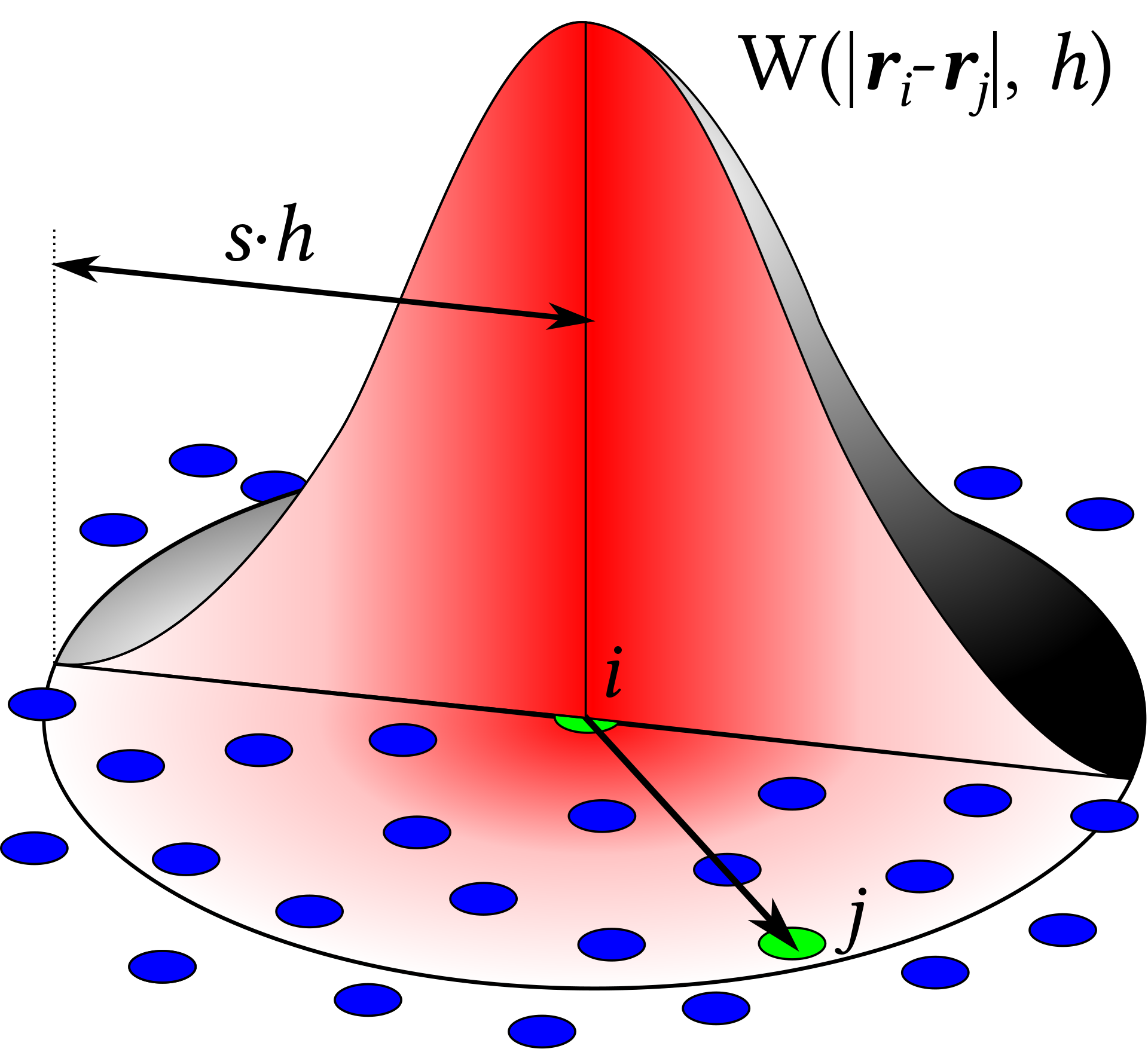
Figure 2.4: A depiction of a smoothing kernel being applied to a discrete set of particles. This image was uploaded to Wikipedia by the user Jlcercos and is licensed under Creative Commons. Here the circles represent the particles, $h$ the smoothing length, and the 3D curve represents the value of the smoothing kernel for all points in space.

For those who are more mathematically inclined, I will briefly provide a more technical description of the smoothing method used for SPH. Readers who are interested in learning more are encouraged to look at Section 5 of [43], as ChaNGa’s implementation of SPH follows closely with the description provided therein [31]. The method involves using a function called a smoothing kernel to continuously map fluid quantities (provided by the representative particles) to the region of space around the particles [12]. According to this method, the smoothing calculation is given by the equation [15]

$$\langle f(\mathbf{r})\rangle=\int f(\mathbf{r}_{j})W(|\mathbf{r}_{i}-\mathbf{r}_{j}|,h)dV(\mathbf{r}_{j}),$$ (2.9)

where $f(\mathbf{r}_{j})$ is the fluid quantity being mapped onto space (such as density) for a representative particle, $\langle f(\mathbf{r})\rangle$ is its average value computed at location $\mathbf{r}$, $W$ is the smoothing kernel function, and $h$ is the smoothing length [12]. Eq. 2.9 can also be approximated as the following sum over particles [15]

$$\langle f(\mathbf{r}_{i})\rangle=\sum_{j}V_{j}f_{j}W(|\mathbf{r}_{i}-\mathbf{r}_{j}|,h).$$ (2.10)

A depiction of the smoothing process is shown in Fig. 2.4. I should again note that I have only aimed to provide a conceptual overview of SPH as a method of modelling a continuous fluid medium using discretized particles (or “parcels”), and have only provided a brief look into the mathematical machinery underlying this process. I would like to state explicitly that understanding the math is not crucial for understanding this document, but the reader who is interested in learning more can refer to resources such as [43], which provides a much more explicit description of the mathematical process.

2.8 The User’s Perspective

So far this chapter has focused heavily on introducing N-body simulation methods at the conceptual level, and while I have personally found my research into the subject incredibly illuminating, it bears acknowledging that the vast majority of us will actually never write such codes of our own (at least, not from scratch). While I don’t think that this fact necessarily detracts from the value of learning about simulation techniques, it does invite discussion of N-body codes through a more practical lens. In this subsection, I will attempt to provide such a discussion by giving a brief overview of the user’s perspective when running a simulation in ChaNGa.

On the most basic level, assuming that you have a computer with a Linux operating system, running a simulation in ChaNGa requires only three things: the code itself, a parameter file, and an initial conditions file. As previous sections in this chapter have sought to highlight, ChaNGa is an incredibly complicated piece of software. This complexity, as well as that of its dependencies, can –in my experience– lead to considerable difficulties in the installation process. If you have gotten ChaNGa to successfully compile on your machine, be proud! It took me nearly half of my first research summer to accomplish exactly that. For those having trouble getting the software set up, I can only refer you to the github documentation [47] and offer my sympathy.

This chapter has hopefully provided a decent idea of what ChaNGa does, but to briefly summarize: it simulates the gravitational motion and gas dynamics of matter in space, producing results that aim to model galactic and/or cosmological structure. Assuming that you have the code downloaded and installed on your machine, you are well on your way to running your own astrophysical simulations! The next two things you need, as previously noted, are parameter and initial conditions files. The latter of the two is perhaps the easiest to intuitively understand: it is a binary file (i.e. a file that is not human readable) that provides the initial positions and velocities of all particles in the simulation [15], which as you may recall from Equations 2.6-2.8 are crucial for the numerical integration process. These initial conditions are not something that can be arbitrarily assigned, at least not if one is hoping to get accurate results, and must be computed in a manner that approximates observations of the early universe via the CMB (see Sec. 0.6) [15]. In my own research, I have never been personally responsible for generating an initial conditions file, so I will not cover that process here. For discussion on one of the tools used for doing so, as well as the process itself, I would refer the reader to Chapter 1 of Mitchell Burdorf’s 2021 thesis [15]. On a practical level, what is most important to understand about a simulation’s initial conditions file are that 1.) it provides the starting point for the computation by giving position and velocity values for all particles at $t=0$, and 2.) that these values are assigned so as to be approximately consistent with observation.

Figure 2.5: The parameter file of a ChaNGa from AGORA’s Cosmorun Paper (S. Roca-Fàbrega, et al. 917, 64 (2021), arXiv:2106.09738 [astro-ph.GA] ), opened in a text editing program.

The final piece of the puzzle is the parameter file, a human readable file with a .param extension that specifies a number of values (parameters) that are important for the computation. Fig. 2.5 depicts a ChaNGa parameter file opened in a text editing program on a Linux machine. As you can see in the figure, all parameters (minus a few notable exceptions) are named such that their data type is specified by their first letter: b for boolean, i for int, and d for double. Some parameters worth noting are dLambda which represents the cosmological constant $\Lambda$ (for more information see Ch. 29 of [2]), dHubble which represents the Hubble Constant $H_{0}$ (again, refer to [2]), nSteps which gives the number of time steps to be performed before the simulation ends, and iOutInterval which gives the number of time steps between simulation outputs. Unlike the initial conditions file, since parameter files are human readable, values can be input by hand. However, it should be explicitly noted that, much like the initial conditions, parameters are chosen with physical realism in mind.

Once the user has a working version of ChaNGa, an initial conditions file, and a parameter file, performing the simulation is simply a matter of running the program, which itself involves a terminal command specifying the number of processor cores to use, as well as the location and name of the parameter file (note that the name of the initial conditions file is specified as one of the parameters).

Chapter 3 Visualization and Analysis Tools

This chapter primarily concerns tools and methods for data visualization and analysis. I should note that, while I will be introducing a number of the tools and techniques used to analyze data in this project, I will not be going into much detail on how they are used (for instance, which commands perform which operations). My goal here is to present an introduction to the important aspects of data analysis rather than providing a guide for how to replicate my results. I would direct the reader who is interested in learning how to use these tools to their respective online documentation libraries [48] [49], where you can find guides for performing different kinds of analysis at varying levels of complexity. These are the resources I used when I was getting started, and it is my opinion that the quality and comprehensiveness of their pedagogy eliminate the need for me to try to guide the reader through their use.

3.1 Data Visualization - yt

The first analysis tool I will discuss, which serves as a foundation for the analytical work for this project (and in fact many other in computational astrophysics and similar fields), is a piece of software called yt. When an N-body code such as ChaNGa performs a simulation, it outputs data in the form of binary “snapshot” files containing information on all the quantities being tracked by the simulation at a given time (or redshift). Unsurprisingly, these files can contain a great deal of data (consider, for instance, the TNG simulations [22], some of the snapshots from which contain terabytes of information), but as they are encoded in binary (and are therefore not human readable), we need a way to extract the information in order to interpret it. This is where yt comes in. yt [50] is an open-source python package which allows the user to perform visualization and analysis on volumetric data sets (that is, data sets that represent a volume of three dimensional space), which is precisely the kind of data set output by simulation codes!

The first thing that yt does when loading a volumetric data set is create a specialized data object containing all the information it reads off of the binary file (I should note that from this point forward, when I use the term “data object” I am likely referring to precisely this python class) [48]. This information is stored in what is known in the language of yt as a “field.” A yt field represents some spatially varying quantity related to the data being loaded, such as gas temperature or density [48]. The package distinguishes between two types of field, native fields and derived fields. Native fields can be thought of as those inherent to the data set, they are quantities which the simulation specifically tracked and consecutively stored in the data output. These are fields that are described by the documentation as “existing externally” to yt, often being stored on disk rather than in memory, and are accessible but immutable with yt [48]. Derived fields are those that yt computes using other fields that are already present in the data object (most often, native fields). This is convenient for accessing quantities which a simulation doesn’t directly track, but are nonetheless relevant, or simply more reasonable to work with, in the context of the analysis being performed. There are a number of derived fields that yt calculates automatically when loading a data set, but the package also enables the user to define their own derived fields to add to the yt data object [48]. While the creation of derived fields is obviously an integral part of the yt package, for the purposes of this thesis there is no need to go into any greater detail. For the reader who is interested in creating their own derived fields and/or in learning more about how yt loads and handles data, I would suggest having a look at the extensive online documentation that exists for the package [48].

To briefly reiterate, yt reads binary simulation data files and creates a specialized data object through which the user is provided access to a number of data fields corresponding to physical quantities tracked within the simulation [48]. From here, it would reasonable to wonder what exactly one does with this data object and its constituent fields. After all, the process by which yt reads and consecutively organizes data – impressive though it may be – would be for naught it it did not enable the user to the go on and perform meaningful analysis with said data. And herein lies the true power of yt: it not only provides access to the contents of non-human-readable simulation files, it also provides a robust framework for extracting meaning from the raw information therein [50].

Among yt’s more notable data analysis features is the ability to filter data, either by field value (e.g. selecting all gas above a certain temperature threshold) or spatially using geometric objects such as boxes, spheres, and lines (e.g. selecting only the data within a spherical section of the total volume) [48]. In the context of this project, yt’s feature of filtering data spatially was particularly useful, as the simulation snapshots I had covered distances many times larger than the radius of the galaxy that I was examining. Using a yt sphere centered at the galaxy, I was effectively able to “focus in” on a smaller, more relevant volume, the scale of which also made the galaxy easier to make out visually (see Fig. 3.1).

Mention of being able to make out features within simulation data visually foreshadows another crucial ability granted by yt, that being data visualization. There are a variety of means by which yt allows the user to visualize data, but those most relevant to this particular project are slice plots, projection plots, and phase plots [48]. Creating a yt slice plot involves taking either the full data set volume or a subvolume selected using one of the geometric spatial features discussed in the previous paragraph (e.g. a spherical subvolume centered at a galaxy), slicing that volume with some intersecting plane, and plotting some relation between field values for points within that plane [48]. Projection plots function similarly in that they begin with defining some plane that intersects the volume (or subvolume), but rather than plotting data only for points within that plane yt projects all data within the volume onto the specified plane, either by integrating or summing over all field values along the lines perpendicular to said plane [48]. One thing I feel I should highlight, especially for readers overwhelmed with some of the more technical language in the previous few sentences, is that primary functional difference between projection and slice plots is what they represent spatially. Slice plots represent data within a two dimensional cross-section of the volume, as though you took an incredibly thin slice out of space and had a look at what was going on just in that slice. Projection plots, on the other hand, give information about some field quantity throughout the whole 3D volume. The process of projecting data quantities can be thought of as similar to “flattening,” as though you smushed down the data volume to an incredibly thin data-patty.

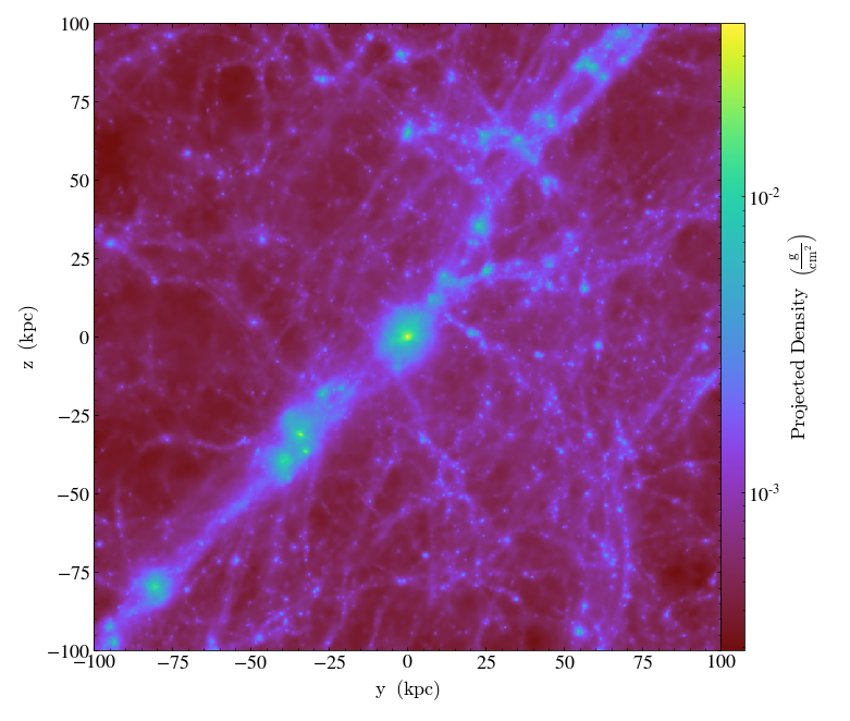
Figure 3.1: A plot of gas density projected on the $y$-$z$ plane for an AGORA Cal IV data set.

yt projection plots are particularly in that they provide a glimpse into what your data actually “looks” like. For instance, the gas density projection plot depicted in Fig. 3.1 gives a good at-a-glance impression of how the matter is distributed throughout the data set volume. The resulting image is not dissimilar from what you would expect to see if the simulated volume was real, and you were looking at it through a telescope. Because of this, one of the first things I usually do when looking at a new data set in yt is create a gas density projection plot to try to get a better idea of the kinds of astrophysical features I’m dealing with, and where they are. By extension, these plots are also incredibly useful when writing about or presenting on computational work, as it requires relatively little effort on the part of the audience to understand what a density projection plot is conveying to them [25]. I should also note that because of their ease of interpretation, it is common practice to use density projection plots to demonstrate results, as exhibited by [17] and [25].

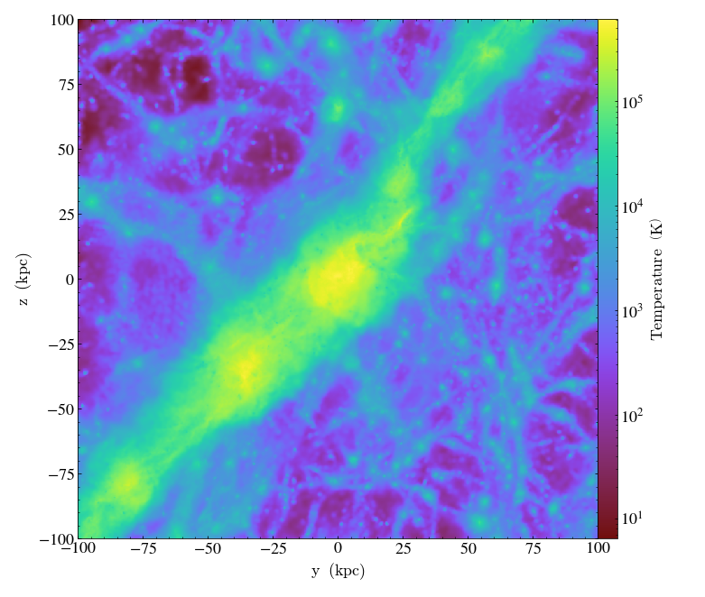
Figure 3.2: A plot of gas temperature projected on the $y$-$z$ plane for the same data set and region depicted in Fig. 3.1.

Though gas density projection plots are an incredibly useful way of visualizing simulation data, and are among the most common one is likely to encounter in the literature, they are far from the only kind of projection plot that yt is equipped to produce. On the contrary, yt’s projection plot function doesn’t limit the user on which data fields they specify to be projected, so – at least in theory – one could create a yt projection plot of just about any data field. As an example, Fig. 3.2 depicts a projection plot of the same region as the gas density plot in Fig. 3.1, but instead of density, the quantity being projected is gas temperature.

It should be noted that yt treats datasets from particle-based codes differently than it does for grid-based codes (see Sec. 2.7 for a discussion on these two approaches) [50]. This dichotomy is discussed further in Sec. 3.2, but readers are also encouraged to look at Sec. 2.1 of [51] for more details on this difference.

3.2 Comparison with Observation - trident

In the previous section, we discussed the use of yt to perform visualization and analysis of the volumetric data in simulation output files. To these ends, yt is invaluable due to the level of control it grants the user and its portability across multiple different simulation codes [50]. However, data from observational studies naturally do not take the same form as simulation output files. Spectroscopic data, for instance, takes the form of light intensity and wavelength measurements, whereas simulation data takes the form of numerical quantities tracked over the simulated volume. Since one of the primary goals of N-body simulations in astrophysics is to perform comparisons against observational results, researchers are left with the often daunting task of finding ways to make such comparisons in a meaningful way given their volumetric outputs.

Luckily for us, in the case of comparing simulation results with those of spectroscopic studies, there is a tool called trident that was created precisely for the purpose reconciling these two types of data. trident [51] is a python library that takes advantage of yt’s portability to produce synthetic spectroscopic absorption data (specifically, quasar absorption, see Sec. 1.2.2) using output files from a rather impressive list of modern simulation codes [51]. Essentially, trident allows the user to define two points within the volume of their 3D dataset (for convenience I will refer to these as the “source” point and “viewing” point), and produces an absorption spectrum that represents what an observer at the viewing point might expect to see if they pointed a spectroscope at a quasar situated at the source point. Note that we add the qualifier “synthetic” (or sometimes “mock”) to the word “spectrum” to distinguish the data that trident produces from real-world observational data. It is precisely trident’s capacity to produce such spectra that makes it such a powerful analytic tool, as it allows users to perform more direct comparisons against observation without making them perform any of the (rather painful) calculation and data manipulation that goes into producing synthetic spectra [51].

From the perspective of the user, creating a synthetic spectrum with trident is simply a matter of specifying which ion species to consider (e.g. Mg, in which case absorptions from Magnesium and all of its ions will be included in the spectrum), then defining the start (source) and end (viewing) points of the sightline, with additional (but uncomplicated) steps such as adding simulated noise to get the spectrum to more closely resemble observational data [49]. trident also allows the user to specify real-world observational equipment for outputs to “mimic” in terms of features such as wavelength range [49]. For instance, users can specify that they want the synthetic spectrum to look like one that might be obtained from the G130M grating of Hubble’s Cosmic Origins Spectrograph (COS) [49], in which case the output spectrum would exhibit features characteristic of that grating such as its 1150-1149 $\mathrm{\SIUnitSymbolAngstrom}$ wavelength range [52]. Additionally, users can specify their own custom wavelength ranges that don’t necessarily correspond to a particular piece of instrumentation [49]. This was particularly useful in my case, as the redshift of the simulation dataset that I used was such that absorption features would not be detectable in the wavelength ranges of the COS’s far ultraviolet modes [52]. Instead, I was able to determine appropriate wavelength ranges for the dataset I was using through the equation [49]

$$\lambda_{\text{obs}}=(1+z)\lambda_{\text{rest}},$$ (3.1)

which gives the absorption wavelength observed at redshift zero ($\lambda_{\text{obs}}$) for an absorption feature with rest wavelength $\lambda_{\text{rest}}$ produced by a material at redshift $z$.

While trident is a remarkably simple tool from the user’s perspective, it should come as no surprise that it is doing a significant amount of non-trivial computation under the hood in order to produce its synthetic spectra. Though an in-depth discussion of trident’s code method is beyond the scope of this project, there are certain aspects of the process that feel important to highlight for the sake of providing a sufficiently robust qualitative understanding of how trident operates. For readers interested in some of the finer details about how trident operates, I would suggest having a look at the method paper [51].

3.2.1 Accounting for missing ions

I have thus far introduced trident’s purpose: to generate synthetic absorption spectra with volumetric simulation data, but in order to properly understand how trident does this, and whether we can trust its results, I must address a particularly significant challenge – one born primarily out of the pragmatic realities of modern computation – that trident must overcome to achieve this end. As discussed in Sec. 0.4, absorption spectra are the result of measuring the intensity of light after it passes through intervening material between source and observer. Recall that certain sets of absorption features (intensity “dips”) are associated with specific atomic species and ion stages, with each species and stage having its own characteristic absorption wavelengths. Thus, one crucial aspect of spectroscopy is identifying the elements associated with the absorption features present in a measurement [2]. The problem that emerges from generating synthetic spectra using simulation data is that there isn’t perfect correspondence between what is present in a simulation and what exists in the physical universe. I am specifically talking about the presence of chemical elements in the simulation. While most simulations will explicitly track lighter elements such as hydrogen and helium, it is often infeasible from a practical standpoint to keep track of each element we would like to consider for the purposes of analysis (let alone all elements in the universe) [51]. So while knowing the abundance of metals and their ions throughout the volume of a simulation dataset is crucial for producing high-fidelity synthetic spectra, it is simply not reasonable for a simulation to track that level of information and the ionization physics necessary to produce it while also performing the gravitational and hydrodynamic calculations characteristic of modern N-body codes (see Ch. 2) [51].

trident’s solution to this dilemma is to extrapolate the presence of any missing ions desired for generating spectra from whatever ion data fields that have been tracked by the simulation. To do so, trident makes the assumption that the number density of the $i$th ion of an element $X$ is given by [51]

$$n_{X_{i}}=n_{X}f_{X_{i}},$$ (3.2)

where $f_{X_{i}}$ is the ionization fraction associated with that particular ion. It should be noted that the ionization fraction is not a constant, and operating under the assumption of ionization equilibrium (as trident does), its value is dependent on temperature, density, and the nature of the radiation field responsible for ionization [51]. This means that it, too, is a value that must be computed, which unfortunately is not a trivial task. Often, simulations modelling ionization are needed in order to get a sense of appropriate values for the ionization fraction [51]. Naturally, trident’s usefulness would be drastically limited if it forced users to run additional computationally-intensive ionization simulations every time they attempted to create a synthetic spectrum, so trident comes pre-packaged with all the information it needs to determine the ionization fraction for the ions of all elements up to Zn (the 30th element on the periodic table) [51]. In more technical terms, trident is equipped with a set of data tables that it uses to look up pre-computed ionization fraction values given various parameters such as temperature and redshift. The data in these tables are the result of simulations performed using the CLOUDY [19], a code used for simulating photoionization.

To recap, when trident encounters a dataset that contains the field for a required atom but is missing fields for one or more of its ionization states, it uses Eq. 3.2 to estimate the presence of the missing ions throughout the dataset volume, then adds a new field containing that information, effectively “populating” the volume (or a specific section of the volume) with the missing ions. However, it is feasible (and, in fact, not unlikely) that the dataset in question comes from a simulation that didn’t track the presence of a particular atom. In such cases, $n_{X}$ is missing from the dataset, so trident makes the estimate [51]

$$n_{X}=n_{H}Z\left(\frac{n_{X}}{n_{H}}\right)_{\odot},$$ (3.3)

where $n_{H}$ is the number density of hydrogen, $Z$ is metallicity, and $(n_{X}/n_{H})_{\odot}$ is the solar abundance of the atom in question.

Using Equations 3.2 and 3.3, trident is able to estimate the spatial number density of all elements up to atomic number 30 so long as the dataset being used has a field corresponding to hydrogen. trident also has methods for producing spectra in the case that a dataset from a simulation that did not track the presence of any element (i.e. not even hydrogen) [51], but simulations containing no elemental data are not discussed in this thesis (and, in fact, are not particularly common in the professional research scene), so the process that trident undergoes to estimate the presence of hydrogen when no such data is available is beyond the scope of this document (though the interested reader is encouraged to have a look at the method paper [51]).

3.2.2 Adding missing ions

I mentioned in the previous section that, once trident has produced its estimates for the density of each relevant ion, it “populates” the dataset with that ion by adding a corresponding yt field. What I have glossed over in this description is the rather nuanced process by which trident goes about accomplishing this task. In general, there are two types of datasets that trident interacts with: those originating from grid-based simulation codes (AMR) and those originating from particle-based codes (SPH) (see Sec. 2.7). As discussed in Ch. 2, these two types of code represent matter differently (as particles or as a density grid, as their names imply). The way that their output data files store information reflects this dichotomy. Since trident works with both types of data files, it must somehow resolve this discrepancy, which, as it turns out, is done by piggybacking off of yt [51]. yt was originally designed as a visualization tool specifically for the AMR code ENZO ([53]) [50], and though its current version is incredibly versatile in terms of the kinds of codes it can do visualization for, it still favors a grid-based paradigm in handling data [51]. As such, when loading a dataset from an SPH simulation, yt actually converts the particle data into a variable-resolution grid structure using an Octree structure similar to that discussed in Sec. 2.3.

Unfortunately, trident’s ion_balance module (the element of the code responsible for generating and adding missing ion fields) has to undergo a more computationally intensive process for SPH datasets than for AMR datasets [51]. In the latter case, since the data were always in grid-format, trident can only consider grid cells along the path of the quasar sightline, meaning that ion_balance doesn’t have to consider the entire simulation volume, which saves a significant amount of computation time [51]. In the case of SPH, however, only considering the presence of ions along the line of sight can lead to significant errors [51], meaning that trident must first create missing ion fields for the entire SPH volume before depositing them into their appropriate grid cells in the yt Octree conversion [51]. This process adds to computation time, but not unreasonably so, and the avoidance of additional errors is certainly worth the cost.

3.2.3 Synthetic Spectra

Once the dataset has been populated with the appropriate ion fields by ion_balance, trident traverses the user specified sightline from the start point to end point, depositing absorption profiles onto a “raw” spectrum (Fig. 3.3) according to the elements encountered along the way and their physical properties (temperature, etc.) [51]. The precise method by which this is accomplished is beyond the scope of this document, but involves a process in spectroscopy known as a Voigt profile calculation. Readers can learn more about the absorption depositing process in Sections 2.4 and 2.5 of the trident method paper [51].

Once the absorption features have been deposited onto the raw spectrum, users are able to add additional features that would be present in observationally obtained spectra, such as a quasar source spectrum and Milky Way foreground [49]. The result of this process in the context of an Enzo dataset is depicted in Fig. 3.4.

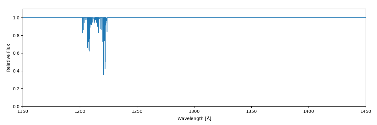
Figure 3.3: A “raw” spectrum produced using an Enzo dataset according to the annotated example on trident’s documentation website: https://trident.readthedocs.io/en/latest/. The ion fields considered are H, C, N, O, and Mg. Absorption features can be seen in the 1150 to 1250 Angstrom range.

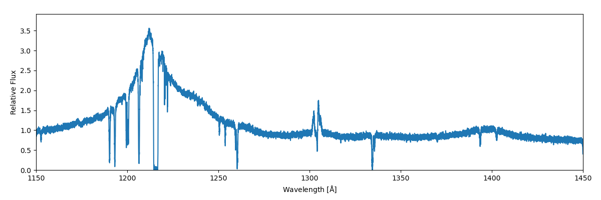
Figure 3.4: The same spectrum depicted in Fig. 3.3, with the addition of a quasar background and Milky Way foreground. Source: https://trident.readthedocs.io/en/latest/.

Fig. 3.5 depicts a comparison between an observationally obtained spectrum [54] and a synthetic spectrum produced in trident [51] using an Enzo dataset [26]. While it is interesting to note the qualitative similarities between these two graphs, it is arguably more important to note that both exhibit crucial similarities with respect to major absorption features [51], such as those occurring just before the 1255 Angstrom point, as well as around 1260 Angstroms. These major features can be seen distinctly in the upper left sub-graphs of the two plots, which show the spectra zoomed-in to the wavelength range 1250-1275 Angstroms. This figure provides a crucial demonstration of trident’s viability as a tool for facilitating comparison between results from computational and observational studies [51].

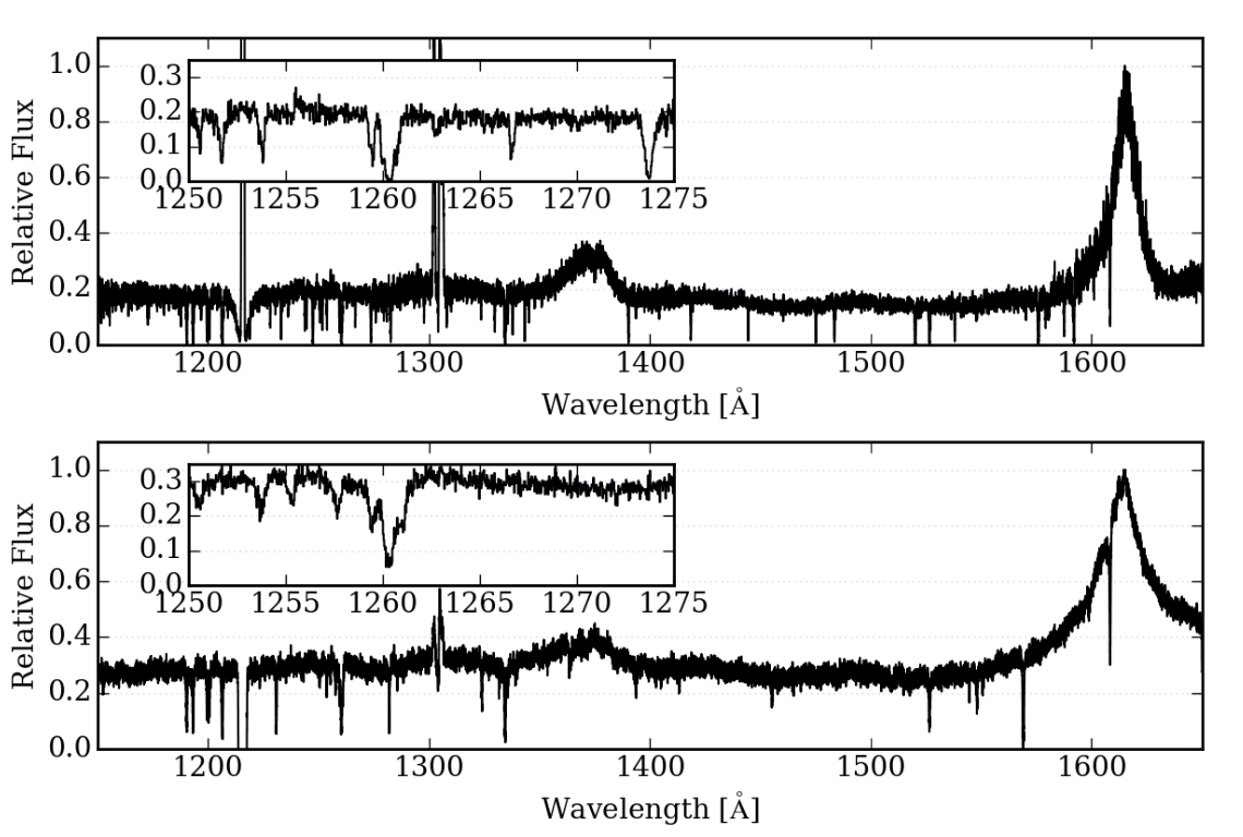
Figure 3.5: A comparison between an observed quasar absorption (top) spectrum and one generated using trident (bottom) at similar redshifts ($z\sim 0.3295$). The observed spectrum was obtained using the Cosmic Origins Spectrogaph on board the Hubble space telescope, and was made publically available by (C. W. Danforth, et al. 817, 111 (2016), arXiv:1402.2655 [astro-ph.CO] ). The synthetic spectrum was produced in trident using data from an Enzo simulation (B. D. Smith, E. J. Hallman, J. M. Shull, and B. W. O’Shea, 731, 6 (2011), arXiv:1009.0261 [astro-ph.CO] ). This figure was borrowed from the trident method paper (C. B. Hummels, B. D. Smith, and D. W. Silvia, 847, 59 (2017), arXiv:1612.03935 [astro-ph.IM]).

Chapter 4 Results

The results of this thesis were primarily demonstrative of trident’s viability as a tool for future work at Reed. Using an output file from a ChaNGa simulation performed as part of AGORA’s third code comparison paper [25] at redshift $z\sim 4$, I was able to produce a series of synthetic quasar absorption spectra with trident. There are a number of problems with these spectra that will need to be addressed in future work before meaningful comparison against observational data can be performed. These issues are discussed in this section, and are also summarized in Ch. 5.

Figure 4.1: An initial synthetic quasar spectrum generated using a ChaNGa data snapshot from (S. Roca-Fàbrega, et al. 917, 64 (2021), arXiv:2106.09738 [astro-ph.GA]) with a sightline spanning the body diagonal of the cubic simulation volume. The horizontal axis represents wavelength in Angstroms.

Fig. 4.1 depicts the first quasar absorption spectrum that I was able to obtain with trident using the AGORA data [25]. This being an incredibly early test of trident’s compatibility with the dataset, I rather arbitrarily decided to define my start and end points such that the sightline would span the length of the simulation volume’s body diagonal, cutting directly through the galaxy (located at the origin). The spectrum was specifically produced with H, C, N, O, and Mg as the specified contributing ion species. I selected the wavelength range of “detection” so that the spectrum would include all possible absorption features associated with the ion species present (see Appendix A for the code I used to determine this wavelength range). This spectrum represents my first successful attempt at using trident on a ChaNGa dataset, and essentially serves as a “proof-of-concept” that students at Reed can use simulation data from ChaNGa in tandem with trident for the purposes of analysis. That being said, there are a number of obvious problems with this spectrum. First, the wavelength range I chose does not correspond to either the far ultraviolet mode (diffraction gratings in the range of 1150-1230 $\mathrm{\SIUnitSymbolAngstrom}$) or the near ultraviolet mode (diffraction gratings in the range of 1700-3200 $\mathrm{\SIUnitSymbolAngstrom}$) of COS [52] [55], which is one of the primary pieces of observational equipment used in contemporary surveys of the CGM [8] and so far the only piece of instrumentation whose measurements trident is equipped to mimic [49]. This problem effectively arises from the fact that the lowest redshift data I had available to me at the time of writing was at $z\sim 4$, whereas CGM surveys via COS (such as COS-Halos [56] [57]) generally probe low-redshift galaxies at $z<1$ [56] [8]. In essence, in order to get results that are even comparable to those that might be obtained using COS, absorption features need to be redshifted into the UV range which would require lower redshift simulation data.

Another issue with the result depicted in Fig. 4.1 is the low flux to noise ratio it exhibits. This issue is so severe that, at the graph’s current scale, one cannot make out any distinct absorption features.

In an attempt to address the issues with my initial graph, I was more judicious in choosing both the sightlines and the wavelength ranges for my later results. Figures 4.2, 4.3, 4.4, and 4.5 show synthetic spectra obtained from trident using the same ChaNGa dataset. The sightlines that produced these spectra had impact parameters of 30 kpc, 50 kpc, 100 kpc, and 500 kpc respectively, and all had length 600 kpc. The parameters of the first two were selected to be relatively consistent with Iryna Butsky’s work using trident with ChaNGa datasets [58], while the latter two were chosen simply to see whether greater impact parameters would have a meaningful affect on the noisiness of the resulting spectrum. In all four cases, the wavelength range was chosen by applying Eq. 3.1 to the maximum and minimum “measured” wavelengths in Fig. 3.4 in the hopes of getting a narrower range that would also include a number of absorption features. As with my preliminary graph (Fig. 4.1), all four of these graphs exhibit high levels of noise with relatively low flux, and no absorption features can be discerned from visual inspection.

It is my belief that the issue presented by the flux to noise ratios in my findings emerges as a result of the high redshift of the simulated galaxy, since redshift is one of the primary differences between the dataset used in this project and the data used to produce the graph in Fig. 3.4, as well as the primary difference between the former and other studies using trident such as [18]. An alternative explanation could be that the issue somehow arises from differences between codes. The graph depicted in Fig. 3.4 comes from a simulation with the code Enzo [53] and [18] uses ART [59], both of which are grid-based (AMR) codes, whereas ChaNGa is an SPH code. Thus, the treatment of fluid dynamics constitutes another major difference between the three datasets. However, there are a number of reasons why I suspect this is not the explanation for the issues with my results. First, the data I am using was produced by AGORA for a paper comparing results from a number of simulation codes at either side of the SPH-AMR dichotomy (including the code used for Fig. 2.7, that used in [18], and ChaNGa) [25]. This paper did report differences among the codes with respect to the CGM properties they produced, but these differences were largely relegated to CGM kinematics, which would not seem to justify the extreme differences between my results and those shown in Fig. 3.4. Additionally, analysis of the CGM in a ChaNGa simulation via trident is something that has been done before: it is the subject of Ch. 4 of [58]. In the case of [58], however, the simulation file used was at $z<0.25$ [58]. In fact, low redshift appears to be a common characteristic among most CGM analyses using trident. The Enzo simulation that produced Fig. 3.4 had a redshift of $z\approx 0.006$, and the data used by [18] was at $z\sim 1$. Because of this relative consistency with respect to redshift, it is my belief that future inquiries into the simulated CGM at Reed should use lower redshift data. If this does not eliminate the aforementioned issues with my results, it will at least rule out high redshift as a culprit.

Figure 4.2: A spectrum resulting from a quasar sightline with a length of 600 kpc and an impact parameter of 30 kpc from the center of the galaxy. The horizontal axis represents wavelength in Angstroms. Only ion species of H, C, N, O, and Mg are considered during spectrum generation. Data obtained from the ChaNGa simulation published in (S. Roca-Fàbrega, et al. 917, 64 (2021), arXiv:2106.09738 [astro-ph.GA]).

Figure 4.3: A spectrum resulting from a quasar sightline with a length of 600 kpc and an impact parameter of 50 kpc from the center of the galaxy. The horizontal axis represents wavelength in Angstroms. Only ion species of H, C, N, O, and Mg are considered during spectrum generation. Data obtained from the ChaNGa simulation published in (S. Roca-Fàbrega, et al. 917, 64 (2021), arXiv:2106.09738 [astro-ph.GA]).

Figure 4.4: A spectrum resulting from a quasar sightline with a length of 600 kpc and an impact parameter of 100 kpc from the center of the galaxy. The horizontal axis represents wavelength in Angstroms. Only ion species of H, C, N, O, and Mg are considered during spectrum generation. Data obtained from the ChaNGa simulation published in (S. Roca-Fàbrega, et al. 917, 64 (2021), arXiv:2106.09738 [astro-ph.GA]).

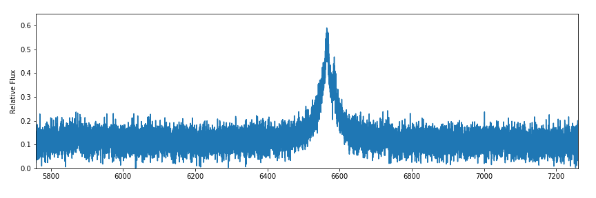
Figure 4.5: A spectrum resulting from a quasar sightline with a length of 600 kpc and an impact parameter of 500 kpc from the center of the galaxy. The horizontal axis represents wavelength in Angstroms. Only ion species of H, C, N, O, and Mg are considered during spectrum generation. Data obtained from the ChaNGa simulation published in (S. Roca-Fàbrega, et al. 917, 64 (2021), arXiv:2106.09738 [astro-ph.GA]).

Chapter 5 Conclusion and Future Work

This document has provided an overview of the missing baryon problem, its relation to the CGM, and the role that N-body simulations can play in furthering our understanding of the mystery (Ch. 1). Additionally, I have provided a conceptual outline of ChaNGa [31], a modern SPH N-body code (Ch. 2), as well as discussions regarding analysis and visualization of simulation data with yt [50] and trident [51] (Ch. 3). As presented in Ch. 4, my results from generating synthetic absorption spectra with trident using ChaNGa data are less than satisfactory, particularly in terms of noisiness and low relative flux. Since contemporary research into the CGM appears to focus largely on low-redshift galaxies commonly with $z\lesssim 1$ in both observational [56] [57] [8] and computational [18] [58] contexts, it is very possible that future work related to this project could benefit from using lower-redshift data. This could also lead to ease of comparison with observational data, since COS, a major tool in modern spectroscopic studies of the CGM [8], is best suited for observing the CGM of low-redshift galaxies [52]. Ultimately, despite their issues, my results do provide good justification for further inquiries into the CGM at Reed, since they demonstrate that trident can be used in tandem with ChaNGa to produce synthetic quasar absorption spectra.

Possible extensions to the project largely center around applying the principles and tools I have presented in order to perform CGM analysis. As previously noted, future work would likely benefit from lower-redshift data. Fortunately, the AGORA simulation from which I acquired my data is planned to run down to a redshift of $z\sim 2$ for work related to future a publication [25], and it is possible that a Reed student could request access to this data for use in a thesis project. While AGORA’s target redshift for the upcoming paper is still larger than the $z\lesssim 1$ that is commonly encountered in the literature, it does come much closer that the $z\sim 4$ data that I used. It would be interesting to see whether results obtained from $z\sim 2$ simulation data would prove more satisfactory than those presented here.

Alternatively, future students could combine my work with that of Mitchell Burdorf [15], who wrote a thesis in 2021 in which he presents results from a ChaNGa cosmological simulation. Burdorf suggests performing a Zoom-in simulation as a possible extension of his work, and his thesis provides an excellent starting point for research into accomplishing just that. If a student was able to build off of Burdorf’s thesis by performing a Zoom-in simulation at Reed to a low enough redshift, they could then feasibly use yt and trident to perform an analysis of the CGM.

Assuming a student is able to get less noisy data with distinct absorption features by using trident on simulation data, they could then attempt to to extract physical information in a manner that imitates observational techniques, as suggested in [51], through a procedure known as Voigt profile analysis. The trident method paper [51] points to [60] and [61] as appropriate resources for understanding algorithms that can used to extract Voigt profile information from synthetic data produced using trident.

Finally, successful application of Voigt profile analysis to a trident spectrum could be extended into a project involving analysis of randomly generated sightlines through a simulated galaxy’s CGM. This procedure is used to account for the fact that scientists on Earth do not have control the sightlines that can be used for CGM analysis in the real universe, and more information can be found in [18] as well as in Ch. 4 of [58], with the latter providing a good description of the algorithm used to produce random sightlines. Those who are not interested in writing their own code for such a project can take advantage of quasarscan [62], the documentation for which can be found at https://quasarscan.readthedocs.io/en/latest/index.html.

Appendix A Determining Wavelength Range for Custom Spectra

This appendix contains the code from a file that I wrote to help find custom wavelength ranges that would capture all potential absorption features for a specified set of ion species within a provided dataset. The code uses Eq. 3.1, and takes advantage of a file in trident’s directory tree called lines.txt. This file provides a table of absorption features for an extensive set of ions in their rest frame (i.e. without redshift), and can be found from the trident directory at trident/data/line_lists/lines.txt. This code functions by reading lines.txt in order to create a dictionary called absorption_dict that is indexed by element name (e.g. ‘Mg’), and whose entries are two-tuples representing the minimum and maximum wavelengths of absorption features associated with the ion species of that element. This dictionary is then used by a function called findShiftedLambda() that takes two arguments: data, which is a data file loaded into yt via the yt.load() function, and element, which is a character array representing the names of elements whose ion species are to be considered (e.g. ‘H’ or ‘Mg’).

⬇

1# File: specrange.py

2#

3

4import yt

5import trident

6

7# Ranges of rest wavelengths for absorption features:

8#

9# <Element> : [<min_wavelength>, <max_wavelength>]

10#

11# Obtained from "lines.txt" on the trident GitHub page.

12#

13

14line_list = trident.__file__[:-11] + "data/line_lists/lines.txt"

15

16f_lines = open(line_list).readlines()

17

18absorption_dict = {}

19

20for line in f_lines[1:]:

21 line = line.split(None)

22 try:

23 absorption_dict[line[0]].append(float(line[2]))

24 except KeyError:

25 absorption_dict[line[0]] = [float(line[2])]

26

27for elem in absorption_dict:

28 absorption_dict[elem] = (min(absorption_dict[elem]),

29 max(absorption_dict[elem]))

30

31

32# Function for determining the wavelength range of

33# absorption features, taking into account current redshift.

34# Takes inputs "data" (YT data set) and "element" (string

35# representing an element in the lambda0 dictionary).

36#

37lambda0 = absorption_dict

38

39def findShiftedLambda(data, element):

40 z = data.current_redshift

41 lambda_min = (1 + z) * lambda0[element][0]

42 lambda_max = (1 + z) * lambda0[element][1]

43 return([lambda_min, lambda_max])

References

- Thornton [2004] S. T. Thornton, Classical dynamics of particles and systems. (Brooks/Cole, Belmont, CA, 2004), 5th ed., ISBN 0534408966.
- Carroll [2007] B. W. Carroll, An introduction to modern astrophysics (Pearson Addison-Wesley, San Francisco, 2007), second edition. ed., ISBN 0805304029.
- Griffiths [2013] D. J. D. J. Griffiths, Introduction to electrodynamics (Pearson, Boston, 2013), fourth edition. ed., ISBN 9780321856562.
- [4] Radio frequency radiation and cell phones, URL https://www.fda.gov/radiation-emitting-products/cell-phones/radio-frequency-radiation-and-cell-phones.
- Taylor [2015] J. R. J. R. Taylor, Modern physics for scientists and engineers. (University Science Books, Mill Valley, California, 2015), second edition / john r. taylor, chris d. zafiratos, michael a. dubson, university of colorado, boulder. ed., ISBN 9781938787751.
- Griffiths [2018] D. J. D. J. Griffiths, Introduction to quantum mechanics (Cambridge University Press, Cambridge, United Kingdom, 2018), third edition. ed., ISBN 9781107189638.
- Olmsted [2002] J. Olmsted, Chemistry (Wiley, New York, 2002), 3rd ed., ISBN 0471390712.
- Tumlinson et al. [2017] J. Tumlinson, M. S. Peeples, and J. K. Werk, Annual Review of Astronomy and Astrophysics 55, 389 (2017), 1709.09180.
- Freese [2017] K. Freese, International Journal of Modern Physics D 26, 1730012-223 (2017), 1701.01840.
- Carroll [2004] S. M. Carroll, Spacetime and geometry : an introduction to general relativity (Addison Wesley, San Francisco, 2004), ISBN 0805387323.
- Bertone and Hooper [2018] G. Bertone and D. Hooper, Reviews of Modern Physics 90, 045002 (2018), 1605.04909.
- Cummings [2020] B. A. Cummings, Bachelor’s thesis, Reed College (2020).
- Sparke [2000a] L. S. Sparke, Galaxies in the Universe : an introduction (Cambridge University Press, New York, 2000a), ISBN 0521592410.
- American Physical Society [2002] American Physical Society, June 1963: Discovery of the cosmic microwave background (2002), URL https://www.aps.org/publications/apsnews/200207/history.cfm?
- Burdorf [2021] M. Burdorf, Bachelor’s thesis, Reed College (2021).
- [16] R. Davé, What’s going on in the circumgalactic medium?, URL https://online.kitp.ucsb.edu/online/bblunch/dave/.
- hoon Kim et al. [2016] J. hoon Kim, O. Agertz, R. Teyssier, M. J. Butler, D. Ceverino, J.-H. Choi, R. Feldmann, B. W. Keller, A. Lupi, T. Quinn, et al., The Astrophysical Journal 833, 202 (2016), URL https://doi.org/10.3847%2F1538-4357%2F833%2F2%2F202.
- Strawn et al. [2021] C. Strawn, S. Roca-Fàbrega, N. Mandelker, J. Primack, J. Stern, D. Ceverino, A. Dekel, B. Wang, and R. Dange, MNRAS 501, 4948 (2021), 2008.11863.
- Ferland et al. [2017] G. J. Ferland, M. Chatzikos, F. Guzmán, M. L. Lykins, P. A. M. van Hoof, R. J. R. Williams, N. P. Abel, N. R. Badnell, F. P. Keenan, R. L. Porter, et al., Rev. Mexicana Astron. Astrofis. 53, 385 (2017), 1705.10877.
- Haardt and Madau [2012] F. Haardt and P. Madau, ApJ 746, 125 (2012), 1105.2039.
- Mo [2010] H. Mo, Galaxy formation and evolution (Cambridge University Press, Cambridge ; New York, 2010), ISBN 9780521857932.
- Naiman et al. [2018] J. P. Naiman, A. Pillepich, V. Springel, E. Ramirez-Ruiz, P. Torrey, M. Vogelsberger, R. Pakmor, D. Nelson, F. Marinacci, L. Hernquist, et al., Monthly Notices of the Royal Astronomical Society 477, 1206 (2018), URL https://doi.org/10.1093%2Fmnras%2Fsty618.
- Geller and Huchra [1989] M. J. Geller and J. P. Huchra, Science 246, 897 (1989).
- Rantala [2014] A. J. Rantala, Master’s thesis, University of Helsinki (2014).
- Roca-Fàbrega et al. [2021a] S. Roca-Fàbrega, J.-H. Kim, L. Hausammann, K. Nagamine, A. Lupi, J. W. Powell, I. Shimizu, D. Ceverino, J. R. Primack, T. R. Quinn, et al., ApJ 917, 64 (2021a), 2106.09738.
- Smith et al. [2011] B. D. Smith, E. J. Hallman, J. M. Shull, and B. W. O’Shea, ApJ 731, 6 (2011), 1009.0261.
- Ryden [2021] B. S. Ryden, Interstellar and intergalactic medium, Ohio State astrophysics series (Cambridge University Press, Cambridge, United Kingdom, 2021), ISBN 1108478972.
- Maoz [2016] D. Maoz, Astrophysics in a nutshell, In a nutshell (Princeton, N.J.) (Princeton University Press, Princeton, New Jersey, 2016), second edition. ed., ISBN 9780691164793.
- qua [a] Cosmos - the sao encyclopedia of astronomy: Quasar, (accessed: 24 Apr. 2022), URL https://astronomy.swin.edu.au/cosmos/q/quasar.
- Schaye [2015] J. Schaye, in IAU General Assembly (2015), vol. 29, p. 2250900.
- Menon et al. [2015] H. Menon, L. Wesolowski, G. Zheng, P. Jetley, L. Kale, T. Quinn, and F. Governato, Computational Astrophysics and Cosmology 2, 1 (2015), 1409.1929.
- Einstein [1916] A. Einstein, Annalen der Physik 354, 769 (1916), ISSN 0003-3804.
- Franklin [2022] J. Franklin, An introduction to general relativity (2022), course Notes, Physics 414.
- Quinn et al. [1997] T. Quinn, N. Katz, J. Stadel, and G. Lake, Time stepping n-body simulations (1997), URL https://arxiv.org/abs/astro-ph/9710043.
- Springel [2005] V. Springel, MNRAS 364, 1105 (2005), astro-ph/0505010.
- Barnes and Hut [1986] J. Barnes and P. Hut, Nature 324, 446 (1986), ISSN 1476-4687, URL https://doi.org/10.1038/324446a0.
- [37] Cos 126 programming assignment: Barnes-hut galaxy simulator, URL https://www.cs.princeton.edu/courses/archive/fall03/cs126/assignments/barnes-hut.html.
- [38] D. Harrison, The multipole expansion, URL https://phys.libretexts.org/Bookshelves/Mathematical_Physics_and_Pedagogy/Mathematical_Methods/The_Multipole_Expansion.
- Stadel [2001] J. G. Stadel, Ph.D. thesis, University of Washington, Seattle (2001).
- Jetley et al. [2008] P. Jetley, F. Gioachin, C. Mendes, L. V. Kale, and T. Quinn, in 2008 IEEE International Symposium on Parallel and Distributed Processing (2008), pp. 1–12.
- [41] Is space infinite?, URL https://www.swinburne.edu.au/news/2021/08/Is-space-infinite-we-asked-5-experts/#:~:text=The%20observable%20universe%20is%20finite,since%20the%20universe%20is%20expanding).
- Schombert [2021] J. Schombert, Hc 441 lecture 5: Cosmological principle (2021), URL http://abyss.uoregon.edu/~js/cosmo/lectures/lec05.html.
- Wadsley et al. [2004] J. Wadsley, J. Stadel, and T. Quinn, New Astronomy 9, 137 (2004), URL https://doi.org/10.1016%2Fj.newast.2003.08.004.
- Hernquist et al. [1991a] L. Hernquist, F. R. Bouchet, and Y. Suto, ApJS 75, 231 (1991a).
- Wadsley et al. [2017] J. W. Wadsley, B. W. Keller, and T. R. Quinn, MNRAS 471, 2357 (2017), 1707.03824.
- Shivamoggi [1998] B. K. Shivamoggi, Theoretical fluid dynamics (Wiley, New York, 1998), 2nd ed., ISBN 0471056596.
- Charles [2022] P. Charles, Changa, https://github.com/N-BodyShop/changa (2022).
- [48] The yt project 4.0.2, URL https://yt-project.org/doc/.
- [49] Trident documentation, URL https://trident.readthedocs.io/en/latest/.
- Turk et al. [2011] M. J. Turk, B. D. Smith, J. S. Oishi, S. Skory, S. W. Skillman, T. Abel, and M. L. Norman, ApJS 192, 9 (2011), 1011.3514.
- Hummels et al. [2017] C. B. Hummels, B. D. Smith, and D. W. Silvia, ApJ 847, 59 (2017), 1612.03935.
- Green et al. [1999] J. C. Green, J. A. Morse, J. Andrews, E. Wilkinson, O. H. W. Siegmund, and D. Ebbets, in Ultraviolet-Optical Space Astronomy Beyond HST, edited by J. A. Morse, J. M. Shull, and A. L. Kinney (1999), vol. 164 of Astronomical Society of the Pacific Conference Series, p. 176.
- Bryan et al. [2014] G. L. Bryan, M. L. Norman, B. W. O'Shea, T. Abel, J. H. Wise, M. J. Turk, D. R. Reynolds, D. C. Collins, P. Wang, S. W. Skillman, et al., The Astrophysical Journal Supplement Series 211, 19 (2014), URL https://doi.org/10.1088%2F0067-0049%2F211%2F2%2F19.
- Danforth et al. [2016] C. W. Danforth, B. A. Keeney, E. M. Tilton, J. M. Shull, J. T. Stocke, M. Stevans, M. M. Pieri, B. D. Savage, K. France, D. Syphers, et al., ApJ 817, 111 (2016), 1402.2655.
- NASA [2017] NASA, Hubble space telescope - cosmic origins spectrograph (2017), URL https://www.nasa.gov/content/hubble-space-telescope-cosmic-origins-spectrograph.
- Prochaska et al. [2017] J. X. Prochaska, J. K. Werk, G. Worseck, T. M. Tripp, J. Tumlinson, J. N. Burchett, A. J. Fox, M. Fumagalli, N. Lehner, M. S. Peeples, et al., ApJ 837, 169 (2017), 1702.02618.
- Goel and Werk [2021] A. Goel and J. Werk, in American Astronomical Society Meeting Abstracts (2021), vol. 53 of American Astronomical Society Meeting Abstracts, p. 135.05.
- Butsky [2021] I. S. Butsky, Phd thesis, University of Washington, Seattle (2021).
- Kravtsov et al. [1997] A. V. Kravtsov, A. A. Klypin, and A. M. Khokhlov, The Astrophysical Journal Supplement Series 111, 73 (1997), URL https://doi.org/10.1086/313015.
- Davé et al. [1997] R. Davé, L. Hernquist, D. H. Weinberg, and N. Katz, ApJ 477, 21 (1997), astro-ph/9609115.
- Egan et al. [2014] H. Egan, B. D. Smith, B. W. O’Shea, and J. M. Shull, ApJ 791, 64 (2014), 1307.2244.
- qua [b] quasarscan, URL https://quasarscan.readthedocs.io/en/latest/index.html.
- [63] PhysicsOpenLab, Atomic spectroscopy, URL https://physicsopenlab.org/2015/11/30/atomic-spectroscopy/.
- Hernquist et al. [1991b] L. Hernquist, F. R. Bouchet, and Y. Suto, ApJS 75, 231 (1991b).
- Sparke [2000b] L. S. Sparke, Galaxies in the universe : an introduction (Cambridge University Press, New York, 2000b), ISBN 0521592410.
- Roca-Fàbrega et al. [2021b] S. Roca-Fàbrega, J.-h. Kim, L. Hausammann, K. Nagamine, J. W. Powell, I. Shimizu, D. Ceverino, A. Lupi, J. R. Primack, T. Quinn, et al., arXiv e-prints arXiv:2106.09738 (2021b), 2106.09738.