The COS-Halos Survey: Metallicities in the Low-Redshift Circumgalactic Medium

Abstract

We analyze new far-ultraviolet spectra of 13 quasars from the $z\sim 0.2$ COS-Halos survey that cover the H I Lyman limit of 14 circumgalactic medium (CGM) systems. These data yield precise estimates or more constraining limits than previous COS-Halos measurements on the H I column densities $N_{\rm HI}$. We then apply a Monte-Carlo Markov Chain approach on 32 systems from COS-Halos to estimate the metallicity of the cool ($T\sim\,10^{4}$ K) CGM gas that gives rise to low-ionization state metal lines, under the assumption of photoionization equilibrium with the extragalactic UV background. The principle results are: (1) the CGM of field $L^{*}$ galaxies exhibits a declining H I surface density with impact parameter $R_{\perp}$ (at $>99.5\%$ confidence), (2) the transmission of ionizing radiation through CGM gas alone is $70\pm 7\%$; (3) the metallicity distribution function of the cool CGM is unimodal with a median of $10^{-0.51}\,Z_{\odot}$ and a 95% interval $\approx 1/50~{}Z_{\odot}$ to $>3~{}Z_{\odot}$. The incidence of metal poor ($<1/100\,Z_{\odot}$) gas is low, implying any such gas discovered along quasar sightlines is typically unrelated to $L^{*}$ galaxies; (4) we find an unexpected increase in gas metallicity with declining $N_{\rm HI}$ (at $>99.9\%$ confidence) and, therefore, also with increasing $R_{\perp}$. The high metallicity at large radii implies early enrichment. (5) A non-parametric estimate of the cool CGM gas mass is $M_{\rm CGM}^{\rm cool}=(9.2\pm 4.3){\rm\;\times\;10^{10}}M_{\odot}$, which together with new mass estimates for the hot CGM may resolve the galactic missing baryons problem. Future analyses of halo gas should focus on the underlying astrophysics governing the CGM, rather than processes that simply expel the medium from the halo.

1 Introduction

Both the conceptualization and discovery of the circumgalactic medium (CGM) was based on the observation of heavy elements (e.g. Mg II, C IV, O VI) along quasar sightlines (e.g. Bahcall & Spitzer, 1969; Bergeron, 1986; Tripp et al., 2000; Chen et al., 2001; Prochaska et al., 2006). As larger surveys and datasets were compiled, it became clear that the present-day CGM accounts for the majority if not all of the detected metal absorption (Cooksey et al., 2010; Prochaska et al., 2011; Bordoloi et al., 2014; Lehner et al., 2015). Consequently, this medium is a major reservoir of heavy elements with a mass rivaling and possibly exceeding that within galaxies (Tumlinson et al., 2011; Werk et al., 2014; Peeples et al., 2014).

Given the diffuse and highly ionized nature of the CGM, its metals must have originated within one or more galaxies and have been transported to the $\sim$100 kpc distances where we observe them. A number of metal transport mechanisms have been proposed, including galactic winds, AGN feedback, accretion, tidal stripping, and ram pressure (e.g. Veilleux et al., 2005; Putman et al., 2012; Oppenheimer & Schaye, 2013). Most of these processes depend sensitively on, and possibly govern, basic galaxy properties such as stellar mass, star formation rates, and chemical enrichment. Gas metallicities provide critical clues to the action of these processes. For example, a high metallicity may indicate that the CGM is polluted by higher mass, chemically-enriched systems. In contrast, a very low metallicity may indicate IGM accretion and/or the by-products of lower mass, satellite galaxies (Lehner et al., 2013). It is plausible that both high and low-metallicity gas coexists in halos from a mixture of ongoing accretion and feedback. If so, the balance may shift with galaxy mass or other properties in ways that reveal the relative importance of the accretion and feedback mechanisms.

Because we use ions of heavy elements to diagnose the physical conditions in CGM gas, its metallicity also bears on its inferred total mass as traced by its H I content. Even if the H I column density ($N_{\rm HI}$) is well constrained, it must be corrected for ionization to derive total surface densities and then integrated to estimate the gaseous halo mass. These ionization corrections are derived from the observed metal lines. Most galaxy-selected studies to date (Prochaska et al., 2011; Stocke et al., 2013; Borthakur et al., 2015; Werk et al., 2014, hereafter W14) have used small, heterogeneous samples dominated by systems bearing large $N_{\rm HI}$ uncertainties caused by saturation in the Lyman series lines that yield lower limits to $N_{\rm HI}$ $\sim 10^{15-16}$ cm^-2. Sightlines penetrating the inner CGM ($R_{\perp}<100$ kpc), where H I column densities are likely higher than this, are particularly affected. This was especially the case for the COS-Halos survey (Tumlinson et al., 2011; Werk et al., 2012; Tumlinson et al., 2013) which analyzed the CGM of $z\sim 0.2$, field $L^{*}$ galaxies at impact parameters $R_{\perp}<150$ kpc. Indeed, our own previous analysis of the COS-Halos survey included $\sim 20$ systems with lower limits to the $N_{\rm HI}$ values based on H I Lyman series analysis (Tumlinson et al., 2013). It is important to obtain precise $N_{\rm HI}$ measurements to fully understand the nature of CGM gas. For example, with access to higher Lyman series lines that precisely constrain $N_{\rm HI}$, Ribaudo et al. (2011b) show that a saturated Ly$\alpha$ absorber at an impact parameter of 37 kpc has a much lower metallicity than its host galaxy and therefore may be an example of cool gas accretion. Recognizing this limitation to the measurement of CGM gas masses and metallicities, we carried out new observations with the Cosmic Origins Spectrograph (COS) on the Hubble Space Telescope (HST) to cover the H I Lyman Limit (LL) of 14 systems. This manuscript describes those observations and the new results that follow.

Section 2 describes the new HST/COS observations and Section 3 presents the new $N_{\rm HI}$ analysis. In Section 4 we perform a new metallicity analysis of the COS-Halos survey using Monte Carlo Markov Chain (MCMC) techniques and Section 5 discusses the primary results. We assume the WMAP9 cosmology (Hinshaw et al., 2013) and report proper distances unless otherwise specified. All of the measurements presented here are available online through the pyigm repository.

Table 1: OBSERVATIONS

Quasar	$z_{\rm em}$	Config.	$t_{\rm eff}^{a}$ (s)
SDSSJ091029.75+101413.6	0.462	G140L	6301
SDSSJ094331.61+053131.4	0.564	G140L	6520
SDSSJ095000.73+483129.3	0.589	G130M	9953
SDSSJ101622.60+470643.3	0.822	G130M	9962
SDSSJ113327.78+032719.1	0.524	G130M	7945
SDSSJ115758.72-002220.8	0.260	G140L	6109
SDSSJ123335.07+475800.4	0.382	G130M	8178
SDSSJ124154.02+572107.3	0.583	G130M	8005
SDSSJ132222.68+464535.2	0.374	G130M	8177
SDSSJ133045.15+281321.4	0.417	G140L	5922
SDSSJ134251.60-005345.3	0.326	G130M	9237
SDSSJ141910.20+420746.9	0.874	G140L	7333
SDSSJ155504.39+362848.0	0.714	G140L	6943

2 Observations and Data Processing

We observed 13 of the COS-Halos sightlines using the COS G140L/1280 setting for 6 quasars and the G130M/1222 setting for 7 quasars (Cycle 20, Program 13033, PI Tumlinson). These two settings were chosen to optimize the short wavelength coverage of the new spectroscopy, extending down the range of the existing COS-Halos data (Program 11598, PI Tumlinson) to $\sim 1000$ Å. Prior to these observations, we had observed and fully analyzed the targeted absorbers as part of the main COS-Halos survey, so that we were able to select the G140L/1280 setting for systems at $z<0.2$ and G130M/1222 for $z>0.2$ (Table 1). The former covers shorter observed-frame wavelengths while the latter offers higher spectral resolution. The observations occurred between 2012 December and 2013 June when COS was in its second lifetime position (LP2).

All of the data were reduced with the CALCOS pipeline (v2.21) using the COS calibration files as of 2014 December. The reduction pipeline settings were customized to use rectangular boxcar extraction windows of 25 pixels and 35 pixels for G140L and G130M spectra, respectively. Detector pulse heights were restricted to $2\leq\mathrm{PHA}\leq 15$ on both detector segments to preserve all source counts while minimizing the detector dark current.These choices preserve spectrophotometric accuracy, while minimizing the background and maximizing data quality.

After extraction, individual sub-exposures were further processed with software developed for the analysis of COS spectra in the low-count (i.e. Poisson) and low-flux ($f_{\lambda}\lesssim 10^{-17}$ erg cm^-2 s^-1 Å^-1) regime (Worseck et al., 2016). Briefly, this software estimates the COS pulse-height-restricted dark current in the science aperture using contemporaneous dark calibration exposures obtained at the same detector voltage and similar space-weather conditions within $\pm 1.5$ months around the date of observation, and coadds subexposures in count space while flagging detector blemishes. The post-processed dark current is accurate to a few percent (Worseck et al., 2016), which is crucial for our measurements of nearly saturated Lyman continuum absorption ($\log N_{\rm HI}\simeq 17.8$).

In G140L spectra scattered geocoronal Ly$\alpha$ emission can be significant (Worseck et al., 2016), but this background component could not be directly estimated, since geocoronal Ly$\alpha$ is not covered in the G140L 1280 Å setup. Based on our analysis of deep G130M data of He II-transparent quasars (Shull et al., 2010; Syphers & Shull, 2014; Worseck et al., 2016) we consider scattered light negligible for G130M spectra at the wavelengths of interest (i.e. $\lambda<$1200 Å). Diffuse Galactic and extragalactic sky emission was not subtracted, as it is much lower than the dark current and scattered light (only 4–10% of the total background; Worseck et al., 2016). Geocoronal oxygen and nitrogen emission was effectively eliminated by considering shadow (orbital night-only) data in the affected wavelength ranges if available. Residual geocoronal emission was flagged after visual inspection.

For final analysis the G140L spectra were binned by a factor of 3 and the G130M spectra by a factor of 4, resulting in a sampling of approximately 2 pixels per resolution element at COS Lifetime Position 2 (G140L: resolving power $\lambda/\Delta\lambda\simeq 2\,000$ at 1150 Å, dispersion $\simeq 0.24$ Å pixel^-1; G130M: $\lambda/\Delta\lambda\simeq 15\,000$ at 1150 Å, dispersion $\simeq 0.04$ Å pixel^-1). For display purposes we computed an approximate $1\sigma$ error array following Worseck et al. (2016), but use the correct asymmetric Poisson error throughout our analysis. Examples of the fully reduced COS spectra are shown in Figure 1, zoomed in on the regions where the Lyman limit absorption occurs. These examples illustrate the range of data quality. The remainder of the sample is shown in the Appendix.

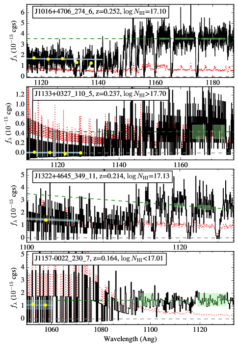
Figure 1: Zoom-in figures of the Lyman limits of four representative CGM systems from the sample. The black line is the HST/COS spectra with corresponding $1\sigma$ error array (red; dotted). The green dashed line is the best-fit continuum model $C_{\lambda}$ and the green shaded regions show the spectral regions used to fit $C_{\lambda}$. The blue line shows the model flux within the Lyman limit region and the shaded blue regions indicate the spectral regions used to estimate $\tau_{\rm LL,\lambda}$. The yellow dots show the mean flux in 5Å bins. These four examples show a range of $N_{\rm HI}$ values and spectral quality characteristic of the full sample, including an upper limit (J1157–0022_230_7) and a lower limit (J1133+0327_110_5).

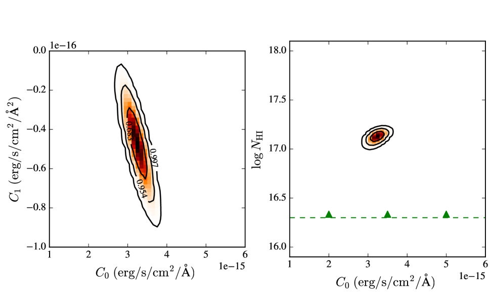
Figure 2: Model constraints on the continuum $C_{\lambda}$ of quasar J1322+4645 with $C_{\lambda}=C_{0}+C_{1}(\lambda-911)$Å (left) and on the H I column density $N_{\rm HI}$ of the CGM associated to the galaxy 349_11 at $z=0.214$ (right). The contours, from inner to outer, indicate the 0.683, 0.954, and 0.997 confidence limits. This system shows an H I Lyman limit opacity near unity which yields a tight constraint on $N_{\rm HI}$. For comparison, the dashed line shows the previous lower limit on $N_{\rm HI}$ based on Lyman series analysis, and the previous upper limit was $N_{\rm HI}<10^{19}\,{\rm cm^{-2}}$ (Tumlinson et al., 2013).

3 $N_{\rm HI}$ Analysis

Our program was designed to provide $N_{\rm HI}$ estimates for 14 systems from the COS-Halos sample through the observations of 13 quasars. These new spectra cover the H I Lyman limit of each system, enabling an estimate of the continuum opacity:

$$\tau_{\rm LL,\lambda}\approx\tau_{912}\left(\,\frac{\lambda}{912\mathrm{\AA}}\,\right)^{2.75}$$ (1)

with $\tau_{912}$ the optical depth at energy $h\nu_{912}=1$ Ryd. From this opacity, one recovers a direct estimate of the total $N_{\rm HI}$ for the system,

$$N_{\rm HI}=\tau_{912}/\sigma(1\,\rm Ryd)\;\;\;,$$ (2)

where $\sigma(1\,\rm Ryd)\approx 6.34{\rm\;\times\;10^{-18}}\,{\rm cm^{2}}$ is the H I photoionization cross-section for 1 Ryd photons. In the following, we adopt the Verner et al. (1996) parameterization of $\tau_{\rm LL,\lambda}$ which gives an accurate representation of the quantum mechanical derivation.

The measurement of $\tau_{\rm LL,\lambda}$ requires an estimate of the quasar continuum $C_{\lambda}$,

$$\tau_{\rm LL,\lambda}=-\ln(f_{\lambda}/C_{\lambda})\;\;\;.$$ (3)

We extrapolate a model for $C_{\lambda}$ based on the observed flux just redward of the Lyman limit. The observed, attenuated quasar flux $f_{\lambda}$ is also partially absorbed by lines associated to the CGM, the Galactic ISM, and other absorption systems along the sightline. This absorption is generally weak and one can identify spectral regions that are likely unabsorbed.

We employed two approaches to estimating $C_{\lambda}$, depending on the absorption redshift and the spectral S/N. For each system we adopt one of these two approaches: (i) a linear fit to $C_{\lambda}$ using select regions of the unabsorbed data, $C_{\lambda}=C_{0}+C_{1}(\lambda-911$Å); and (ii) a constant value, $C_{\lambda}=C_{0}$ fitted to select regions. We adopt the former for data of higher quality based on inspection near the Lyman limit. Examples of our adopted continuum placements are shown in Figure 1. The remaining systems are presented in the Appendix.

For J0943+0531, the LL occurs just blueward of the $\sim 18$Å gap between the COS FUV detector segments, which precludes a direct estimate of $C_{\lambda}$ near the break. We set $C_{\lambda}=C_{0}$ based on the flux measured redward of the gap (at $\lambda\approx 1350$Å) and adopt a large uncertainty. This system has negligible LL absorption and we recover only a conservative upper limit to $N_{\rm HI}$ which is relatively insensitive to $C_{\lambda}$.

After setting the unabsorbed continuum regions, we performed a maximum likelihood analysis to estimate $N_{\rm HI}$. The full model flux $M_{\lambda}$ consists of a continuum $C_{\lambda}$, parameterized by $C_{0}$ and/or $C_{1}$, attenuated by the Lyman limit opacity $\tau_{\rm LL,\lambda}$ set by the free parameter $N_{\rm HI}$ given in Equation 2:

$$M_{\lambda}=C_{\lambda}\,\exp(-\tau_{\rm LL,\lambda})\;\;\;.$$ (4)

From this model flux, the average number of model counts per pixel $\mu_{i}$ was estimated using the known sensitivity function for the instrument and the effective exposure time $t_{\rm eff}$ (Table 1) of each observation. Additionally, we included an estimate of the background counts following Worseck et al. (2016). We assumed a Poisson deviate for the counts in the LL region and Gaussian statistics for the continuum. Formally, the Poisson deviate for the observed counts $m_{i}$ in each pixel of the analysis region is $P_{i}(m_{i};\mu_{i})$. The likelihood function follows simply as $\mathcal{L}=\Pi_{i}P_{i}$.

We calculated the maximum likelihood $\mathcal{L}$ for a large grid covering the allowed space for the continuum parameters and $N_{\rm HI}$. The best values of these three parameters are taken at the maximum $\mathcal{L}$. Errors are estimated by integrating over the grid to assess the cumulative probability. Figure 2 shows the results for a well-modeled system (J1322+4645_349_11); it describes the constraints on the parameters and also their correlation. Analysis of the LL yields only limits to $N_{\rm HI}$ when the opacity is much higher or lower than unity. In these cases, we report one-sided 95% confidence limits for $N_{\rm HI}$ and rely on the Lyman series analysis to further refine the value.

Figure 1 shows the best-fit models of four systems overlaid on the spectra near the LL (the remainder of systems are shown in the Appendix). Table 2 lists the spectral regions used for the Lyman limit and continuum analyses, the best-fit values, and the $68\%$ confidence interval for $N_{\rm HI}$. We have also revisited the Lyman series analysis for the systems with only lower limits on $N_{\rm HI}$. In nearly every case, we have set an upper limit from the absence of damping wings in the Ly$\alpha$ line. These are also provided in the table, and we consider all values in this range equally likely (i.e. we adopt a flat prior).

Table 2: $N_{\rm HI}$ MODELS AND MEASUREMENTS

Galaxy	z	flg${}_{C}^{a}$	$\lambda_{C}^{b}$	$C_{0}$	$\sigma(C_{0})$	$C_{1}$	$\sigma(C_{1})$	$\lambda_{\tau}$	$\log N_{\rm HI}^{c}$	C.L.d
			(Å)	(10-15)		(10-17)
J0910+1014_242_34	0.264	2	[1157.30,1159.95]	0.64	0.02			[1120.0,1150.0]	$16.58$	16.51,16.62
			[1162.68,1165.80]
J0910+1014_34_46	0.143	0							$17.25$	16.00,18.50
J0943+0531_106_34	0.228	2	[1127.04,1132.19]	1.96	0.10			[1090.0,1119.0]	$<16.24$
			[1136.35,1140.84]
J0943+0531_227_19	0.353	3		2.01				[1120.0,1150.0]	$<16.65$
J0950+4831_177_27	0.212	1	[1116.38,1117.77]	5.71	0.15	$-3.02$	0.49	[1095.0,1104.0]	$>17.91$
									18.20	17.90,18.50
J1009+0713_170_9	0.356	0							$18.50$	18.00,19.00
J1009+0713_204_17	0.228	0							$17.50$	16.50,18.50
J1016+4706_274_6	0.252	2	[1161.42,1164.69]	3.57	0.06			[1115.0,1130.0]	$17.10$	17.08,17.11
			[1166.92,1173.34]
			[1176.01,1184.38]
J1016+4706_359_16	0.166	0							$17.50$	16.50,18.50
J1112+3539_236_14	0.247	0							$16.70$	15.80,17.60
J1133+0327_110_5	0.237	2	[1163.83,1167.97]	0.44	0.14			[1110.0,1120.0]	$>17.70$
									18.60	18.54,18.66
J1133+0327_164_21	0.154	0							$16.90$	15.80,18.00
J1157-0022_230_7	0.164	2	[1095.88,1101.43]	1.45	0.48			[1050.0,1063.0]	$<17.01$
			[1118.98,1130.69]
J1233+4758_94_38	0.222	2	[1130.63,1131.36]	4.31	0.15			[1106.0,1111.0]	$16.74$	16.69,16.77
			[1138.68,1142.35]
J1241+5721_199_6	0.205	1	[1110.63,1111.52]	3.71	0.21	$-3.76$	0.57	[1091.0,1098.0]	$>17.83$
									18.15	17.80,18.50
J1322+4645_349_11	0.214	1	[1115.55,1115.86]	3.24	0.10	$-4.69$	0.71	[1100.0,1106.0]	$17.14$	17.10,17.16
			[1119.25,1120.45]
			[1122.41,1124.07]
J1330+2813_289_28	0.192	2	[1102.32,1109.35]	2.02	0.29			[1070.0,1086.0]	$17.03$	16.88,17.11
J1342-0053_157_10	0.227	1	[1131.02,1132.28]	5.29	0.21	$-1.71$	0.53	[1105.0,1117.5]	$>18.04$
									18.50	18.00,19.00
J1419+4207_132_30	0.179	2	[1094.70,1099.28]	3.00	0.24			[1045.0,1074.0]	$16.63$	16.33,16.72
			[1106.57,1110.78]
J1514+3619_287_14	0.212	0							$17.50$	16.50,18.50
J1555+3628_88_11	0.189	2	[1100.62,1105.08]	0.60	0.12			[1057.0,1083.5]	$17.17$	16.91,17.30
			[1108.25,1113.18]

Note. — Units for $C_{0}$ and $C_{1}$ are erg/s/cm²/Å and erg/s/cm²/Ų respecitvely.

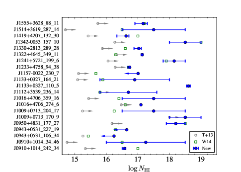
Figure 3: Measurements of $N_{\rm HI}$ including upper and lower limits from the analysis in this paper (blue) compared against previous estimates from H I Lyman series analysis (Tumlinson et al., 2013; Werk et al., 2014, gray circles and green squares, respectively). The new values are in general agreement with the previous estimates and limits.

Figure 3 compares these new $N_{\rm HI}$ measurements with our previous estimates. The Tumlinson et al. (2013) measurements (grey circles) were conservatively derived from analysis of the H I Lyman series while the W14 estimates (green squares) included a prior on the gas metallicity, requiring sub-solar values. The new $N_{\rm HI}$ measurements (blue circles with errors) exceed prior estimates from the Lyman series, or impose a lower limit consistent with the previous measurement.

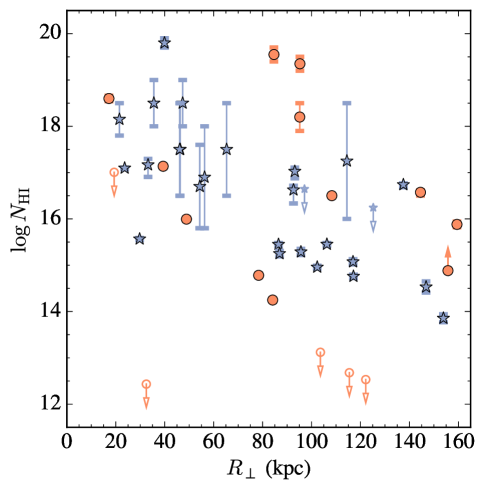
Figure 4: $N_{\rm HI}$ values for the COS-Halos survey versus the projected impact parameter $R_{\perp}$ to the target galaxy. The measurement of each CGM system is coded by the specific SFR (sSFR) such that red circles indicate a sSFR $<$ 10^-11 M_⊙ yr^-1, while blue stars represent galaxies with sSFR higher than this limit. Open symbols indicate non-detections in H I and error bars (typically $<0.1$ dex) are overplotted on detections. Note the high incidence of optically thick gas at $R_{\perp}<60$ kpc and the overall trend to lower $N_{\rm HI}$ at higher $R_{\perp}$. The null hypothesis of no correlation is ruled out at $>99.6\%$ confidence.

Figure 4 presents the updated $N_{\rm HI}$ distribution for the COS-Halos sample as a function of impact parameter and color-coded for the target galaxy’s star-formation rate (Werk et al., 2012). We find a strong anti-correlation between $N_{\rm HI}$ and $R_{\perp}$ across the full sample; a Kendall Tau correlation test including censored data carried out with the ASURV package rules out the null hypothesis at $>99.6\%$ confidence. This suggests a higher characteristic hydrogen density $n_{\rm H}$ closer to the galaxy.

As an aside, we emphasize that the COS-Halos sample exhibits a high incidence of optically thick gas ($N_{\rm HI}\geq 10^{17}\,{\rm cm^{-2}}$) for sightlines penetrating within $\approx 60$ kpc of a field $L^{*}$ galaxy. This implies that long sightlines selected for high redshift and/or bright FUV magnitudes are somewhat biased against the ‘inner’ CGM for luminous galaxies at $z>0.3-0.5$ because the strong LL absorption in the inner CGM severely suppresses the FUV flux.

4 Metallicity Analysis

In this section, we reexamine the metal enrichment of the cool CGM in the COS-Halos sample with two key advances over previous work. First, the new $N_{\rm HI}$ measurements greatly improve the precision of the gas metallicity estimates. Second, we adopt a new methodology for constraining the ionization state based on the techniques described in Fumagalli et al. (2016) (see also Crighton et al. (2015)).

4.1 Methodology

We have used Monte Carlo Markov Chain (MCMC) techniques to compare a grid of plane-parallel, photoionization models parameterized by the gas density $n_{\rm H}$, H I column density $N_{\rm HI}$, and metallicity [Z/H] against the observed ionic column densities of low ionization state metal species (e.g. Si⁺, Si⁺⁺, N⁺). A detailed description of this analysis used to estimate gas metallicities for the COS-Halos sample is provided in the Appendix. From the MCMC chains, we derive probability distribution functions (PDFs) for the model parameters that describe the physical state of the absorbing gas. These provide a more quantitative estimation of the statistical uncertainties than our previous analysis. Table 3 summarizes the main results for the 32 systems analyzed.

Table 3: SUMMARY OF PHOTOIONIZATION MODELING

Galaxy	m${}_{\rm ion}^{a}$	$f^{b}$	$\log N_{\rm HI,min}^{\rm prior}$	$\log N_{\rm HI,max}^{\rm prior}$	$\log N_{\rm HI}$	$\log n_{\rm H}$	[Z/H]
J0401-0540_67_24	2	0	15.42	15.48	15.34, 15.39, 15.45	-3.89, -3.56, -3.30	-0.27, -0.10, 0.15
J0803+4332_306_20	1	0	14.74	14.82	14.61, 14.69, 14.80	-3.82, -3.02, -2.69	-0.48, 0.06, 0.80
J0910+1014_242_34	5	0	16.52	16.63	16.42, 16.52, 16.63	-2.77, -2.59, -2.42	-0.25, -0.17, -0.04
J0910+1014_34_46	4	-3	16.00	18.50	17.45, 17.71, 17.94	-4.03, -3.80, -3.53	-1.77, -1.62, -1.42
J0914+2823_41_27	1	0	15.42	15.48	15.34, 15.40, 15.45	-3.81, -3.36, -3.07	-0.66, -0.44, -0.14
J0925+4004_196_22	8	0	19.40	19.70	19.39, 19.51, 19.65	-4.42, -4.17, -3.88	-0.95, -0.81, -0.66
J0928+6025_110_35	8	0	19.20	19.50	19.13, 19.30, 19.47	-3.11, -2.96, -2.85	-0.40, -0.15, 0.14
J0943+0531_106_34	1	0	15.50	16.57	15.53, 15.94, 16.39	-3.83, -3.36, -2.92	-1.28, -0.70, -0.13
J0950+4831_177_27	7	-3	17.90	18.50	18.03, 18.20, 18.37	-2.98, -2.80, -2.63	-1.01, -0.91, -0.77
J1009+0713_170_9	7	-3	18.00	19.00	18.34, 18.62, 18.84	-2.76, -2.53, -2.39	-0.92, -0.76, -0.61
J1009+0713_204_17	3	-3	16.50	18.50	17.13, 17.26, 17.39	-4.02, -3.81, -3.63	-1.19, -1.03, -0.83
J1016+4706_274_6	6	0	17.08	17.11	17.00, 17.05, 17.10	-3.21, -3.08, -2.98	-0.40, -0.35, -0.30
J1016+4706_359_16	5	-3	16.50	18.50	16.80, 17.74, 18.24	-3.77, -3.39, -3.14	-1.55, -1.23, -0.43
J1112+3539_236_14	2	-3	15.80	17.60	16.20, 16.68, 17.20	-2.81, -2.66, -2.53	-1.46, -0.93, -0.44
J1133+0327_110_5	6	0	18.54	18.66	18.40, 18.52, 18.59	-3.40, -3.20, -2.99	-1.39, -1.27, -1.19
J1220+3853_225_38	2	0	15.82	15.94	15.71, 15.82, 15.90	-4.28, -3.91, -3.60	0.27, 0.67, 1.10
J1233+4758_94_38	5	0	16.70	16.78	16.68, 16.74, 16.80	-3.11, -2.98, -2.84	-0.38, -0.29, -0.18
J1233-0031_168_7	2	0	15.54	15.59	15.42, 15.52, 15.59	-3.80, -3.46, -3.19	-0.23, -0.00, 0.32
J1241+5721_199_6	9	-3	17.80	18.50	18.25, 18.37, 18.44	-3.28, -3.20, -3.13	-0.71, -0.65, -0.59
J1241+5721_208_27	2	0	15.22	15.35	15.09, 15.21, 15.29	-3.41, -3.32, -3.19	0.15, 0.26, 0.41
J1245+3356_236_36	1	0	14.72	14.80	14.60, 14.66, 14.72	-3.84, -3.00, -2.64	-0.57, 0.03, 0.81
J1322+4645_349_11	5	0	17.11	17.17	17.00, 17.05, 17.10	-3.10, -2.97, -2.84	-0.82, -0.70, -0.62
J1330+2813_289_28	6	0	16.91	17.14	16.88, 17.01, 17.12	-2.61, -2.50, -2.41	-0.58, -0.50, -0.41
J1342-0053_157_10	9	-3	18.00	19.00	18.67, 18.82, 18.89	-2.81, -2.75, -2.70	-0.27, -0.20, -0.14
J1419+4207_132_30	6	0	16.43	16.82	16.69, 16.89, 17.07	-2.94, -2.82, -2.70	-0.69, -0.54, -0.42
J1435+3604_126_21	1	0	15.19	15.31	15.07, 15.17, 15.28	-3.90, -3.58, -3.34	-0.10, 0.14, 0.47
J1435+3604_68_12	7	0	19.70	19.90	19.59, 19.73, 19.82	-4.26, -3.76, -3.18	-1.45, -1.31, -1.18
J1514+3619_287_14	2	-3	16.50	18.50	17.20, 17.51, 17.84	-2.63, -2.51, -2.42	-1.27, -1.04, -0.75
J1550+4001_197_23	4	0	16.48	16.52	16.40, 16.45, 16.50	-2.80, -2.75, -2.70	-0.40, -0.35, -0.30
J1555+3628_88_11	6	0	16.97	17.36	17.17, 17.31, 17.46	-3.23, -3.07, -2.93	-0.96, -0.82, -0.71
J2345-0059_356_12	3	0	15.96	16.03	15.82, 15.92, 16.03	-3.68, -3.52, -3.36	-0.02, 0.11, 0.27

Note. — The following systems had insufficient data constraints for an ionization analysis: J0226+0015_268_22, J0935+0204_15_28, J0943+0531_216_61, J0943+0531_227_19, J1133+0327_164_21, J1157-0022_230_7, J1342-0053_77_10, J1437+5045_317_38, J1445+3428_232_33, J1550+4001_97_33, J1617+0638_253_39, J1619+3342_113_40, J2257+1340_270_40.

Note. — The $\log N_{\rm HI},\log n_{\rm H}$ and [Z/H] values are represent the 68% c.l. interval and median of the MCMC PDFs.

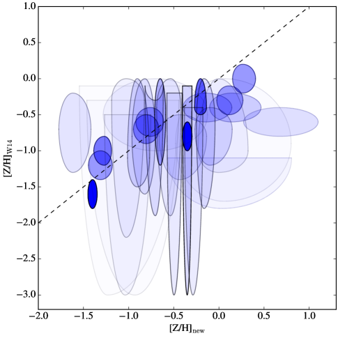
Figure 5: Comparison of the metallicity estimates from this work against the values reported in W14. The plotted ellipses have asymmetric semi-major and semi-minor axes to mimic the asymmetries in the PDFs for [Z/H] and/or limits to the value. Furthermore, the shading indicates the precision in [Z/H] in our new analysis (darker is more precise). Overall, there is good agreement between the two sets of measurements which is expected given both studies assumed photoionization modeling and nearly the same set of ionic column densities. The only significant difference is that the new sample of measurements extends to [Z/H] $>0$ as we have relaxed the prior adopted by W14 restricting the values to solar or lower. The dashed lines denotes a 1-to-1 correspondence between the two sets of measurements.

4.2 Metallicity of the CGM for $L^{*}$ Galaxies

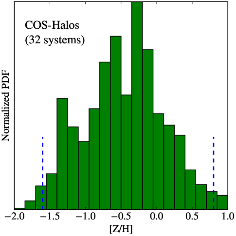
Figure 6: Integrated metallicity PDF for the 32 systems from the COS-Halos dataset with at least one positive detection of a low or intermediate ionic state of a heavy element. This PDF has a median value [Z/H]${}_{\rm median}=-0.51$ dex and a 95% c.l. of $[-1.71,0.76]$, as marked by the blue dashed lines. The data is well-described by a unimodal distribution.

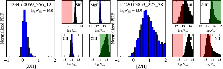
Figure 7: Metallicity PDFs for two systems where 95% of the PDF exceeds 0.5 solar metallicity. Also shown are several of the ionic constraints for each sightline, compared against the model PDFs of $N_{\rm ion}$. Shading is the same as in Figure 20.

From the MCMC analysis, we have generated a metallicity PDF for 32 of the COS-Halos systems with at least one positive detection of a lower ionization state. Figure 5 compares the metallicity measurements for the systems overlapping with W14. In general, there is good agreement between the two analyses. This is expected given that each analysis adopted very similar observational constraints and assumed photoionization equilibrium. The MCMC analysis generally yields a smaller uncertainty than those reported in W14, for several reasons: (a) the more precise measurements of $N_{\rm HI}$ from the new COS data; (b) a conservative approach to uncertainty estimates in W14; and (c) overly optimistic uncertainty estimates from the MCMC analysis. On the latter point, we adopt a minimum systematic uncertainty of 0.3 dex in metallicities due to the over-simplifying assumptions of our photoionization models (e.g. co-spatial gas with a constant density; Haislmaier et al., In prep; Wotta et al., 2016).

Figure 6 shows the combined metallicity PDF of the COS-Halos survey restricted to systems with at least one detected metal transition. The median gas metallicity is high, [Z/H]${}_{\rm median}=-0.51$ dex and the 95% interval is broad, spanning from $\approx 1/50$ solar to $>$3x solar metallicity.

We may conclude that the CGM of field $L^{*}$ galaxies is generally enriched above $\sim 10$% solar. The substantial scatter in these inferred metallicities could come from a range in the mean metallicity of the halos, from varying metallicities within each halo, or both. We discuss these results further in Section 5.2.

4.3 Super-solar CGM Gas

W14 adopted a prior on the gas metallicity that restricted [Z/H] $\leq 0$, i.e. to not exceed solar metallicity. This choice was somewhat arbitrary and was primarily motivated by the large $N_{\rm HI}$ uncertainties in a set of systems with saturated H I Lyman series absorption. In the current analysis, we allow [Z/H] values up to 100x solar to assess the incidence of super-solar metallicities.

Figure 7 shows the ion constraints for two of the four systems that exceed 1/2 solar metallicity at 95% confidence in the MCMC analysis. This subset of high metallicity systems is heterogeneous in terms of data quality and observational constraints but all have $N_{\rm HI}<10^{16}\,{\rm cm^{-2}}$. The combination of low $N_{\rm HI}$ with the positive detection of one or more ions drives the metallicity to a high value.

Of course, the estimated [Z/H] values require significant ionization corrections. Figure 23 of the Appendix shows the corrections required to convert an observed ${N({\rm Si^{++}})}/N_{\rm HI}$ ratio to a [Si/H] abundance for photoionization models with a wide range of $N_{\rm HI}$ and $n_{\rm H}$ values. The figure reveals that the smallest correction is $\approx+2.4$ dex and occurs at a very low gas density (i.e. a very high ionization parameter). For the two systems presented in Figure 7 with a Si⁺⁺ detection, we measure $\log({N({\rm Si^{++}})}/N_{\rm HI})>-2.55$ dex yielding [Si/H] $>-0.2$ dex on the assumption of photoionization equilibrium. We note that similar results apply for collisional ionization equilibrium (CIE). Using the calculations of Gnat & Sternberg (2007), the smallest ionization correction is +2.2 dex. Presently, we have no reason to assert that these lower $N_{\rm HI}$ systems are out of ionization equilibrium. Furthermore, the few cases which exhibit multiple ionization states are well-modeled by the simple equilibrium models. Nevertheless, we caution that low density gas may not be in strict ionization balance (e.g. Gnat & Sternberg, 2007).

In the full sample, 15% of the systems have 90% of their metallicity PDFs above solar, while 25% of the sample has 50% of their PDFs above solar. This implies high enrichment levels at large radii from the central galaxy. We conclude that at least a subset of the CGM surrounding field $L^{*}$ galaxies has a super-solar metallicity (see also Tripp et al., 2011; Meiring et al., 2013).

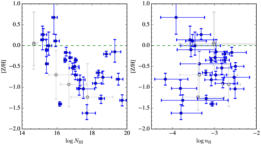
Figure 8: Comparison of intrinsic properties against CGM metallicity. For the H I column density (left-hand panel), there is an apparent anti-correlation with $>99.99\%$ statistical significance. However, [Z/H] does not correlate with the derived gas volume densities (right-hand panel). Grey points indicate systems with very poorly constrained values.

4.4 Intrinsic Correlations

In Figure 8 we present the median [Z/H] values and the 68% confidence intervals for the PDFs of each CGM system against several intrinsic properties of the CGM. From the figure, it is apparent that there is a strong anti-correlation between the measured $N_{\rm HI}$ values and [Z/H]. A Pearson’s correlation test on the plotted values rules out the null hypothesis at $>99.99\%$ confidence. This is driven by the approximately solar metallicity systems with $N_{\rm HI}<10^{16}\,{\rm cm^{-2}}$ (see also Figure 7), the decrease in [Z/H] with $N_{\rm HI}$ for systems having $N_{\rm HI}\approx 10^{17}\,{\rm cm^{-2}}$, and the rarity of [Z/H] $\approx 0$ values at high $N_{\rm HI}$.

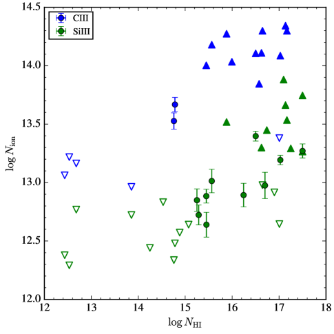
Figure 9: Scatter plot of Si⁺⁺ and C⁺⁺ column densities vs. $N_{\rm HI}$ for the COS-Halos sample. At $N_{\rm HI}>10^{14.5}\,{\rm cm^{-2}}$, nearly every system exhibits a positive detection of one of these two ions. The lower $N_{\rm HI}$ systems, meanwhile, have limits to $N_{\rm ion}$ consistent with the overall trend. Therefore, these limits have little constraining power on the gas metallicity.

Before proceeding, we consider each of these points more carefully. First, the apparent decline in [Z/H] for $N_{\rm HI}=10^{16.5-18}\,{\rm cm^{-2}}$ could be caused by uncertainties in these $N_{\rm HI}$ values combined with the fact that [Z/H] is inversely proportional to $N_{\rm HI}$. However, the systems with $N_{\rm HI}\approx 10^{18}\,{\rm cm^{-2}}$ have PDFs with values toward the low end of their allowed $N_{\rm HI}$ range, which gives higher [Z/H] values. Second, the low incidence of solar metallicity at high $N_{\rm HI}$ is subject to significant sample variance. Figure 8 shows that 2 of 7 systems with $N_{\rm HI}>10^{18}\,{\rm cm^{-2}}$ have [Z/H] $>-0.5$ dex. Adopting binomial statistics, the rate of high metallicity is 0.285 with a 60% uncertainty (i.e. a 100% incidence is nearly allowed).

We also consider whether the preponderance of high metallicity values at lower $N_{\rm HI}$ is a selection effect introduced by our requirement for at least one positive detection of a heavy element transition to perform the metallicity analysis. For low $N_{\rm HI}$ and limited S/N in the data, this cut prefers high metallicities. We assess this possible selection bias as follows. Figure 9 plots the ionic column densities for Si⁺⁺ and C⁺⁺ for the full COS-Halos sample against their $N_{\rm HI}$ values. At $N_{\rm HI}\lesssim 10^{14.5}\,{\rm cm^{-2}}$, there are no detections and these systems may be ignored in this discussion. At $N_{\rm HI}>10^{15}\,{\rm cm^{-2}}$, the detection rate is $>90\%$ implying no selection bias.

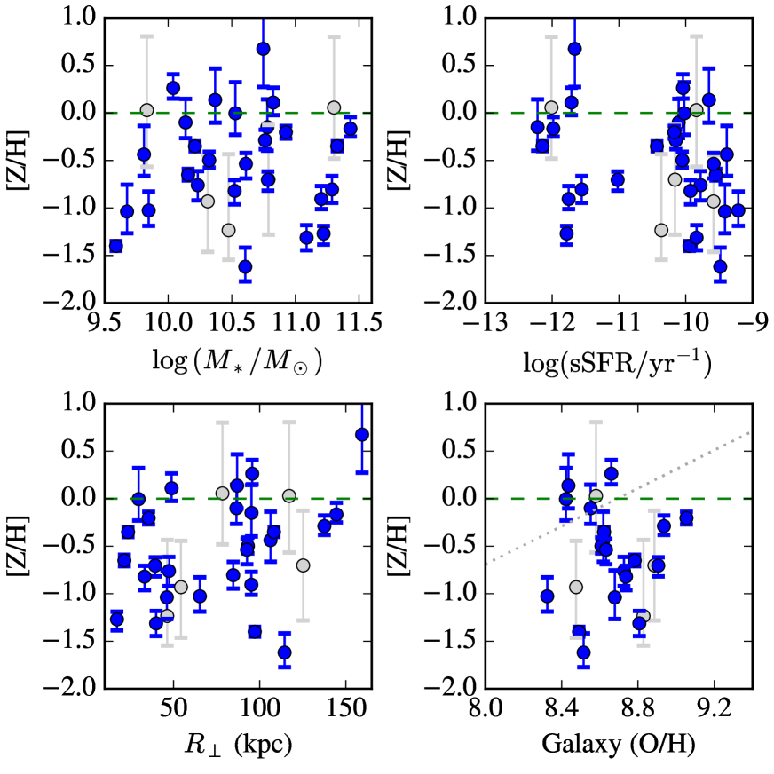
Figure 10: Comparison of the gas metallicity against several extrinsic properties of the CGM systems. There is little evidence for a correlation between [Z/H] and any of these quantities, although there is a weak trend with $R_{\perp}$. This follows from the strong correlations between $N_{\rm HI}$ and $R_{\perp}$ and [Z/H] and $N_{\rm HI}$. Grey points indicate systems with very poorly constrained values.

At $N_{\rm HI}\approx 10^{15}\,{\rm cm^{-2}}$, there are $\sim 3$ systems without a detection of Si⁺⁺ or C⁺⁺. Most of these have ${N({\rm Si^{++}})}<10^{12.5}\,{\rm cm^{-2}}$ ($2\sigma$), which is lower than the typical detection but several have positive C⁺⁺ detections. Furthermore, the addition of a few [Z/H] $\lesssim-1$ systems to Figure 8 at low $N_{\rm HI}$ values would not qualitatively alter the observed trend. We conclude that if one restricts to systems with $N_{\rm HI}>10^{14.5}\,{\rm cm^{-2}}$, then an anti-correlation exists between the enrichment level and the H I column density in the CGM of low $z$, massive galaxies, under the assumption that photoionization equilibrium holds over this range of $N_{\rm HI}$.

4.5 Extrinsic Trends

In Figure 10, we examine trends of [Z/H] with a set of extrinsic parameters. The stellar mass $M_{*}$, specific star formation rate (sSFR), and nebular emission-line metallicity measurements (O/H) are taken from Werk et al. (2012). For the latter, we adopt their M91 calibration.

The [Z/H] vs. $M_{*}$ figure exhibits no hint of an underlying trend. There is, however, a weak, anti-correlation with the specific star formation rate (sSFR; null hypothesis ruled out at $95\%$ for the Pearson’s test) and a tentative positive correlation with impact parameter ($96\%$). The latter follows from two key results of this paper: (i) decreasing $N_{\rm HI}$ values with increasing impact parameters; (ii) an anti-correlation between $N_{\rm HI}$ and [Z/H]. The $R_{\perp}$/[Z/H] correlation is at a lower statistical significance, however, due to the large [Z/H] scatter at all $R_{\perp}$. An anti-correlation between [Z/H] and sSFR may run contrary to the interpretation that the dependence of O VI on sSFR (Tumlinson et al., 2011) is driven by metal-rich outflows (e.g. Stinson et al., 2012).

4.6 Enhanced $\alpha$/Fe

Lau et al. (2016) have recently reported enhanced ratios $\alpha$-chain elements O, Si to Fe relative to the solar abundance in the CGM surrounding massive galaxies at $z\sim 2$. Their analysis is similar to the one presented here: measurements of ionic column densities (primarily low-ion transitions, e.g. O I 1302, Si II 1304) converted to elemental abundances via corrections from constrained photoionization models. Such an $\alpha$-enhancement may be expected for the gas surrounding massive galaxies if the nucleosynthesis is dominated by Type II supernovae. We have compared our unenhanced models against the observed Si/Fe ionic ratios and find no significant inconsistency. At present, we find no evidence for an $\alpha$/Fe enhancement, but caution that the uncertainties may exceed any expected enhancement.

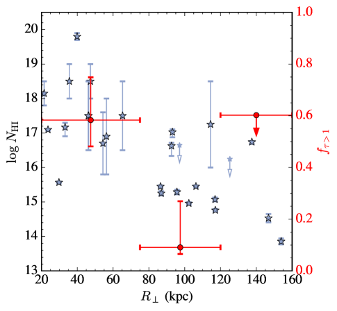
Figure 11: $N_{\rm HI}$ measurements vs. $R_{\perp}$for star-forming galaxies within the COS-Halos survey. Arrows indicate upper limits. Overplotted in red are binned evaluations of $f_{\rm esc}^{\rm CGM}$ the fraction of systems with $\tau_{\rm LL,\lambda}\geq 1$. Uncertainties are standard binomial 68% c.l. intervals while the upper limit corresponds to 95% c.l. While the covering fraction of optically thick gas is high at $R_{\perp}\leq 70$ kpc, a significant fraction of sightlines has low opacity indicating that a non-negligible escape fraction through the CGM of $L^{*}$ galaxies.

5 Discussion

We now discuss in greater detail the implications for several of the main results of this manuscript. Throughout, we focus on the statistical ensemble of COS-Halos measurements, and we remind the reader that these are drawn from a homogeneous sample of sightlines penetrating the CGM of $z\sim 0.2$, field $\sim L^{*}$ galaxies (i.e., $0.3<L/L^{*}<2$) with impact parameters $R_{\perp}<160$ kpc.

5.1 Escape Fraction ($f_{\rm esc}^{\rm CGM}$)

Perhaps the dominant uncertainty in estimates of the $z<1$ EUVB is the contribution from star-forming galaxies (e.g. Haardt & Madau, 2001; Kollmeier et al., 2014). This uncertainty stems primarily from the poor constraints on the escape fraction $f_{\rm esc}$ of ionizing radiation from the hot stars that produce these photons. Most measurements have indicated a nearly negligible value (e.g. Leitherer et al., 1995), but recent work has identified at least a subset of systems with significant leakage (Borthakur et al., 2014; Izotov et al., 2016; Leitherer et al., 2016).

One of the contributing factors to the total $f_{\rm esc}^{\rm T}$ value is the CGM, i.e. the incidence of optically thick gas in galaxy halos. We may assess $f_{\rm esc}^{\rm CGM}$, the escape fraction through the CGM of star-forming $L^{*}$ galaxies at $z\sim 0$, as follows. Figure 11 shows the $N_{\rm HI}$ measurements versus $R_{\perp}$ for the star-forming galaxies of the COS-Halos survey. In three arbitrary $R_{\perp}$ bins we have calculated $f_{\tau\geq 1}$, the fraction of sightlines with $N_{\rm HI}\geq 10^{17.2}\,{\rm cm^{-2}}$ corresponding to a Lyman continuum opacity $\tau_{912}\geq 1$. The $f_{\tau\geq 1}$ values and two-sided confidence intervals (68%) are overplotted on the data. For $R_{\perp}<75$ kpc, $f_{\tau\geq 1}$ likely exceeds 0.5 however $\approx 40\%$ of the sightlines have $\tau_{912}\lesssim 1$. This includes three sightlines with $R_{\perp}\lesssim 30$ kpc, implying that the CGM is not entirely opaque to ionizing radiation.

We may estimate $f_{\rm esc}^{\rm CGM}$ from $f_{\tau\geq 1}$ as follows. First we emphasize that a given CGM sightline from our experiment travels through the entire halo at $R_{\perp}$ but does not sample radii $r<R_{\perp}$. The this means that our dataset only constrains $f_{\rm esc}^{\rm CGM}$ for $r>30$ kpc. And, in contrast to ionizing sources lyat the center of the halo (i.e. within the galaxy), $f_{\tau\geq 1}$ corresponds to approximately twice the opacity that a photon would encounter if emitted from the center. Because $f_{\tau\geq 1}$ is large only in the inner bin, we base our estimate on it alone. Specifically, we approximate $f_{\rm esc}^{\rm CGM}$ as:

$$f_{\rm esc}^{\rm CGM}=1-f_{\tau\geq 1}(R_{\perp}<{\rm 70\,kpc})/2\approx 0.70\pm 0.07$$ (5)

An estimate of $f_{\rm esc}^{\rm CGM}$ for the Milky Way has been performed using surveys of the high velocity clouds (HVCs Weiner et al., 2001; Bland-Hawthorn & Maloney, 2001; Fox et al., 2006; Wakker, 2015). Their analysis indicates $f_{\rm esc}^{\rm CGM}$ of a few to several tens percent which is much smaller than our estimate. This apparent discrepancy suggests that a significant fraction of the opacity is due to gas with $r<30$ kpc, which is consistent with distance estimates for many HVCs (e.g. Thom et al., 2008; Wakker et al., 2008). However, we cannot know how typical the Milky Way is in this regard, or how this opacity varies with galaxy mass. As COS-Halos is not sensitive to $r<30$ kpc, and the fraction of optically thick systems appears to increase rapidly down to and inside this radius, it remains possible that $L^{*}$ galaxies do have small CGM escape fractions.In any case, if the total escape fraction is nearly 0, i.e. $f_{\rm esc}^{\rm T}\ll f_{\rm esc}^{\rm CGM}$, then sources of opacity within the ISM or the first 30 kpc of the CGM dominate.

5.2 Enrichment of the cool CGM

Detections of strong metal lines in $\sim L^{*}$ galaxy halos demonstrate that the CGM is enriched in heavy elements (Bergeron, 1986; Chen et al., 2001). Thus far, however, a robust metallicity distribution function (MDF) has been stymied by small sample sizes, heterogeneous sample selection, large uncertainties in the hydrogen gas content, and ionization corrections. The COS-Halos survey and the new $N_{\rm HI}$ and ionization analyses presented here address these issues, allowing a first estimate of the CGM-MDF.

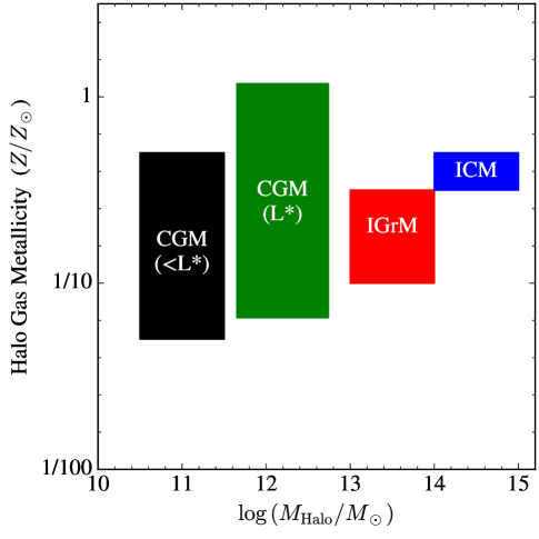
Figure 12: Halo gas metallicity plotted against total halo mass for systems at $z\sim 0$. The measurements were taken from Bordoloi et al. (in prep; sub-$L^{*}$), this work ($L^{*}$), Rasmussen & Ponman (2009; intragroup medium or IGrM), and Maughan et al. (2008; ICM). There is a general trend toward higher halo metallicity with increasing mass although we stress that the individual galaxies show a larger spread.

The primary result from the MDF (Figure 6) is that the cool gas within the CGM exhibits a metallicity exceeding 1/10 solar abundance. The median metallicity, measured from the 32 COS-Halos systems analyzed, is $\approx 1/3$ solar. This requires substantial and likely sustained enrichment from the central galaxy and/or its progenitors. This metallicity roughly matches the values estimated for HVCs in our Galaxy (e.g. Gibson et al., 2001; Collins et al., 2007) and new phenomenological models for the hot halo (Faerman et al., 2017).

While the cases in which the CGM metallicity is higher than the metallicity derived from ionized gas within the galaxies can potentially be understood by invoking metal-enriched outflows (Peeples & Shankar, 2011), the median CGM metallicity is significantly lower than the ISM metallicity (Figure 10; Werk et al., 2012). This indicates that the halo was primarily enriched by stars at an earlier time, when the galaxy itself had lower metallicity, or that metal-rich ejecta were diluted by more metal-poor gas within the halo, and/or lower metallicity gas from accreting satellite dwarf galaxies (e.g. Shen et al., 2013). We encourage the development of chemical evolution models that focus on the CGM.

The median CGM metallicity is also consistent with the enrichment of the hot ($T>10^{6}$K) ‘halo’ gas comprising the intracluster medium (ICM; see Figure 12; Maughan et al., 2008). Indeed, the processes that polluted the CGM of $L^{*}$ galaxies over the past $\sim 10$ Gyr may be the same that enriched the ICM. In this picture, the ICM represents the enriched halo gas stripped from $L^{*}$ galaxies and then shock-heated to the cluster virial temperature (e.g. Matteucci & Gibson, 1995; Sivanandam et al., 2009). In principle, this scenario could be tested by examining the detailed abundance patterns of each. Figure 12 also shows current estimates for the halo gas metallicity of the intragroup medium (IGrM; Rasmussen & Ponman, 2009) and estimates for the CGM of the sub-$L^{*}$ halos probed by the COS-Dwarfs survey (Bordoloi et al., in prep). The IGrM and ICM suggest a trend toward higher metallicity at higher halo mass. The $L^{*}$ galaxies, however, exhibit a large spread that extends even beyond the ICM measurements. Nevertheless, it appears reasonable that the halo gas of individual galaxies can source the IGrM and ICM.

Our analysis detects no evidence for a radial gradient in the gas metallicity. If anything, [Z/H] increases at higher impact parameters (Figure 10). This may conflict with models that envision the modern CGM to be dominated by on-going winds from the central galaxy. Instead, it may favor scenarios where the CGM was polluted by one or more processes long ago (Davé & Oppenheimer, 2007; Ford et al., 2014; Oppenheimer et al., 2016). Of course, this is most evident for the red-and-dead galaxies of COS-Halos which also exhibit a high metallicity CGM (log sSFR $<-11$ in Figure 10).

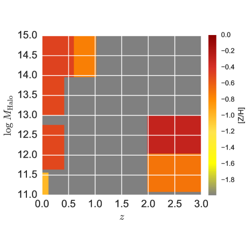
Figure 13: Graphic illustrating current constraints on the CGM enrichment of dark matter halos as a function of mass and redshift. This includes our new results at low-$z$. Ongoing surveys will address the unconstrained areas (colored gray).

We emphasize further that enriched gas is very likely to be present beyond the survey limit of COS-Halos (i.e. at $r>150$ kpc) in both the cool CGM (Zhu et al., 2014) and the highly ionized gas probed by O VI (Prochaska et al., 2011; Johnson et al., 2015). Such widespread and high metallicity implies an enrichment process dominated by activity at early times. One further appreciates that the CGM of bright $z\sim 2$ galaxies also exhibits a high degree of enrichment (e.g. Crighton et al., 2015; Turner et al., 2014; Prochaska et al., 2013; Lau et al., 2016). The terrific puzzle that emerges is whether we are observing the same halo gas at $z\sim 0$ as observed at $z\sim 2$ (see Lehner et al., 2014, for similar considerations but for O VI gas). Figure 13 expresses estimates for the metallicity of the halo gas surrounding halos of a wide range of mass and at varying redshift.

As is evident from Figure 6 (and Figure 12) the CGM MDF for $L^{*}$ galaxies is broad, showing a 68% c.l. interval of $\approx 1$ dex. Despite the large uncertainties to deriving metallicities from the (limited) observations of CGM systems, we contend that the measured scatter includes a significant intrinsic contribution from metallicity variations within halos. This assertion is supported by Figure 9 where one identifies large variations in ${N({\rm Si^{++}})}$ and ${N({\rm C^{++}})}$ at any given $N_{\rm HI}$ value. Furthermore, we have argued for examples of super-solar metallicity (Figure 7) yet expect these are a minority. Unfortunately, we cannot yet test whether the dispersion is intrinsic to individual halos (see Bowen et al., 2016, for progress) – thereby implying inefficient mixing (e.g. Schaye et al., 2007) – or tracks differences between halos. On the latter point, we note no strong trends with stellar mass (Figure 10) that could generate an apparent dispersion. Irrespective of its origin, the measured [Z/H] dispersion places a new constraint on the physical processes that enrich the CGM.

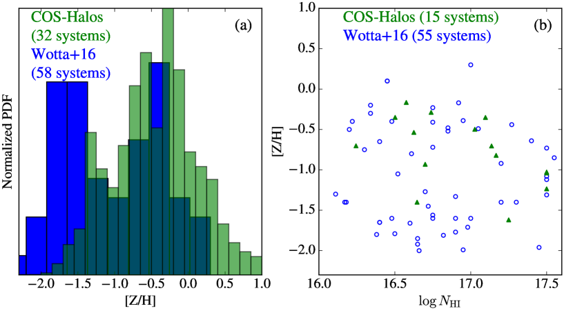
Figure 14: Comparison of the metallicity distribution functions (MDFs) between the CGM of $L^{*}$ galaxies and the optically thick gas traced by $z<1$ Lyman limit systems (LLSs; W16). The left panel shows the complete samples (W16 limits are shown as values in this presentation) while the right panel is restricted to $\log N_{\rm HI}=[16,17.6]$. In both panels we find that the $L^{*}$ CGM overlaps the high metallicity portion of the LLS MDF implying the former gives rise to the latter. Furthermore, we propose that the lower metallicity LLSs might be associated with lower mass galaxies although no apparent trend with stellar mass exists in our sample.

Lastly, we compare our results on the CGM of $L^{*}$ galaxies with the MDF derived for $z<1$ Lyman limit systems (LLSs; Lehner et al., 2013; Wotta et al., 2016), which are also believed to trace the halos of galaxies (e.g. Lehner et al., 2013; Hafen et al., 2016). Figure 14 compares the MDF of the LLS analyzed by (Wotta et al., 2016, hereafter W16) against the full COS-Halos sample. The COS-Halos MDF overlaps the higher metallicity measurements of the LLSs but shows a smaller incidence of low metallicity gas. W16 have emphasized that the MDF of the LLSs is bimodal when one restricts to the lower $N_{\rm HI}$ systems, aka partial LLSs or pLLSs. In the right panel of Figure 14, we restrict both samples to $N_{\rm HI}=10^{16}-10^{17.6}\,{\rm cm^{-2}}$ and see similar results to the full samples; overlap at high [Z/H] and fewer CGM sightlines with [Z/H] $<-1$. Performing a two-sided Kolmogorov-Smirnov test on the sets of [Z/H] measurements rules out the null hypothesis at $\approx 95\%$ that the two samples are drawn from the same parent population.

We propose that a substantial fraction of the highly enriched, optically thick gas traced by LLSs is associated with $L^{*}$ galaxies. Indeed, adopting the comoving number density $n_{L^{*}}$ of $L>0.5L^{*}$ galaxies at $z\sim 0.3$ from Loveday et al. (2015) and $R_{\rm CGM}=150$ kpc, and assuming the covering fraction of the CGM to pLLSs to be $f_{\rm CGM}^{\rm pLLS}=0.2$, we predict an incidence:

$$\ell(X)=n_{\rm L^{*}}\,\pi R_{\rm CGM}^{2}\,f_{\rm CGM}^{\rm pLLS}\approx 0.1\;\;.$$ (6)

This is $\approx 50\%$ of the incidence of $\tau\geq 2$ LLSs ($N_{\rm HI}\geq 10^{17.5}\,{\rm cm^{-2}}$) estimated by Ribaudo et al. (2011a). We conclude that the enriched halos of $L\approx L^{*}$ galaxies can explain the majority of high metallicity LLSs observed by Lehner et al. (2013) and W16. First results on associating the LLSs to galaxies support this assertion (Lehner et al., 2013), but not without exception.

The other important conclusion from Figure 14b is that the low metallicity pLLSs are unlikely to arise from the CGM of $L^{*}$ galaxies. There are, however, two caveats: (1) the gas could arise primarily at $R_{\perp}>150$ kpc, i.e. beyond the COS-Halos survey design (although high $N_{\rm HI}$ values are more rarely observed at these separations Lehner et al., 2013); and (2) the median redshift of the W16 sample is $\tilde{z}\approx 0.6$, i.e. sampling an epoch 3.3 Gyr earlier than the COS-Halos sample. At a constant $N_{\rm HI}$, one expects to probe higher overdensities in our present-day universe. Nevertheless, we suggest that the low metallicity gas observed by W16 is associated with the halos of lower mass galaxies (e.g. Ribaudo et al., 2011b), and further caution that it need not be linked to gas freshly accreting from the IGM.

Table 4: CGM MASS

$R_{\perp}^{a}$	$\log M_{\rm CGM}^{\rm Ann,i}$	$\sigma(\log M_{\rm CGM}^{\rm Ann,i})$
(kpc)	($M_{\odot}$)	($M_{\odot}$)
20	8.9	0.3
30	9.9	0.4
40	9.4	0.3
50	8.2	0.3
60	10.0	0.3
70	7.3	0.3
80	10.6	0.4
90	9.2	0.2
100	8.2	0.2
110	10.2	0.4
120	9.0	0.3
130	8.6	0.3
140	8.1	0.3
150	8.4	0.3

5.3 Revisiting the Cool CGM Mass ($M_{\rm CGM}^{\rm cool}$)

The primary result of W14 was an estimate of the cool gas mass of the CGM (see also Stocke et al., 2013), as assessed from a simple log-linear fit to estimates of $N_{\rm H}$ versus $R_{\perp}$. This analysis was subject to substantial uncertainty stemming from the large uncertainties on $N_{\rm HI}$, the systematic uncertainties of ionization modeling, and the simplicity of this $N_{\rm H}(R_{\perp})$ profile. With our analysis, we have greatly improved the $N_{\rm HI}$ measurements and we provide a more robust assessment of the error in photoionization modeling. These may provide a more accurate and precise estimate of $M_{\rm CGM}^{\rm cool}$. In addition, we introduce a new non-parametric approach to the mass estimate.

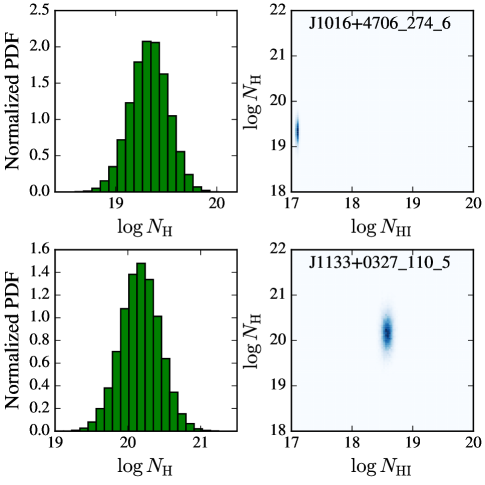
Figure 15: The left panels show the total hydrogen column density $N_{\rm H}$ probability distribution functions (PDFs) for two systems representative of the full sample. These are derived from the MCMC analysis and also include a 0.15 dex Gaussian uncertainty from estimated systematic error. The right panels show the MCMC results in the $N_{\rm H}$/$N_{\rm HI}$ plane.

Figure 15 shows the $N_{\rm H}$ PDF for two representative systems, which differ greatly in the precision of their $N_{\rm HI}$ measurements. The PDFs were generated from the MCMC ionization analysis described in the Appendix and include an additional 0.15 dex Gaussian systematic uncertainty. This systematic error dominates the PDF for J1016+4706_274_6 which otherwise exhibits a very narrow $N_{\rm H}$ distribution. The uncertainty for J1133+0327_110_5, however, is dominated by the error in $N_{\rm HI}$; one notes a relatively tight correlation between the two properties.

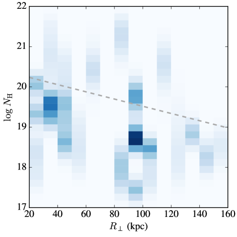
Figure 16: Two-dimensional histogram of the PDFs for the 32 systems of the COS-Halos survey analyzed here. The bin sizes are 10 kpc in $R_{\perp}$ and 0.17 dex in $N_{\rm H}$. The darker colors reflect both the sharpness of the PDF and the number of systems at a given $R_{\perp}$ bin. The gray dashed line shows a fit to the $N_{\rm H}$ values versus $R_{\perp}$ from W14.

By collating the $N_{\rm H}$ PDFs for the 32 systems analyzed from the COS-Halos survey, we may generate a 2D histogram in $N_{\rm H}$-$R_{\perp}$ space (Figure 16). Note that each system contributes equally to the histogram and that several bins contain more than one system, i.e. the ‘maximum’ at $R_{\perp}\approx 90$ kpc and $N_{\rm H}\approx 10^{18.8}\,{\rm cm^{-2}}$ reflects both a sharply peaked PDF in that bin and the fact that several systems contribute. A qualitative assessment of Figure 16 suggests a declining $N_{\rm H}$ value with increasing $R_{\perp}$ but also large $N_{\rm H}$ scatter both within and between the $R_{\perp}$ bins. Future studies (e.g. the CGM² Gemini Large Program, PI Werk) should reduce the current sample variance.

We now offer a non-parametric estimate of the mass $M_{\rm CGM}^{\rm cool}$ of the cool CGM within 160 kpc. In $R_{\perp}$ bins of $\Delta R=10$ kpc starting at 20 kpc, we estimate a ‘best’ $N_{\rm H}$ value $N_{\rm H,j}^{\rm best}$ and its uncertainty $\sigma(N_{\rm H,j}^{\rm best})$. Each bin then contributes an annular mass:

$$M_{\rm CGM}^{\rm Ann,i}=m_{p}\,\mu\ N_{\rm H,j}^{\rm best}\,\pi[(R_{\perp,j}+\Delta R)^{2}-R_{\perp,j}^{2}]\;\;\;,$$ (7)

with $\mu\approx 1.3$ the reduced mass correcting for Helium. The total mass is trivially estimated by summing over the annuli:

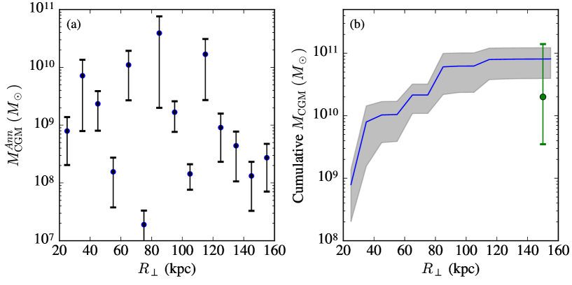
Figure 17: (a) Estimated mass in annuli of 10 kpc width for the CGM, estimated from the COS-Halos survey. The uncertainty is estimated from a bootstrap analysis (see text). (b) The estimated cumulative mass of the cool CGM gas. The green point with error bar shows the mass estimate (with conservative bound) from W14 to $R_{\perp}=150$ kpc.

$$M_{\rm CGM}^{\rm cool}=\sum\limits_{j}M_{\rm CGM}^{\rm Ann,i}\;\;.$$ (8)

The challenge remains, however, to estimate $N_{\rm H,j}^{\rm best}$ and its uncertainty. There are at least three statistics one can derive from a single $N_{\rm H}$ PDF: (1) the geometric mean $N_{\rm H,j}^{\rm best}=10^{\langle\log N_{\rm H}\rangle}$; (2) the true mean $N_{\rm H,j}^{\rm best}=\langle 10^{\log N_{\rm H}}\rangle$; and (3) the median. In practice, the first and last estimators yield similar results because the PDFs are relatively symmetric in log space. The true mean, however, yields systematically higher values ($\approx 0.3$ dex). Presently, it is difficult to argue convincingly for any of these prescriptions (on statistical or physical grounds), but consider the following. In the $R_{\perp}=[80,90]$ kpc bin there are a pair of systems with $N_{\rm H}$ PDFs that peak at $\approx 10^{18}$ and $10^{21}\,{\rm cm^{-2}}$. Unless the high $N_{\rm H}$ system is a true statistical fluke, the average $N_{\rm H}$ value in that annulus must be much closer to it. Therefore, we proceed with the true mean and caution that the resultant mass estimate is especially sensitive to sample variance.

Figure 17a shows the $M_{\rm CGM}^{\rm Ann,i}$ measurements vs. $R_{\perp}$. One finds a relatively flat profile which declines at higher $R_{\perp}$ values. We have estimated the uncertainty in each annulus by a two-fold bootstrap procedure. First, we randomly sample the 32 systems allowing for duplication. Then we randomly sample each system’s $N_{\rm H}$ PDF allowing for duplication. We perform this exercise for 10,000 realizations and show the standard deviation on the $M_{\rm CGM}^{\rm Ann,i}$ values (Table 4).

Figure 17b shows the cumulative mass profile. Similarly, the uncertainty shows the standard deviation in the cumulative mass at each $R_{\perp}$ bin. Altogether we estimate $M_{\rm CGM}^{\rm cool}=(9.2\pm 4.3){\rm\;\times\;10^{10}}M_{\odot}$ to $R_{\perp}=160$ kpc. Examining Figure 17, it appears the mass has converged although this should be confirmed by analyses at higher $R_{\perp}$ (e.g. extending to the virial radius). Our new estimate is consistent with the lower limit established by W14. It implies, as further emphasized in the next section, that cool gas in the halo is a terrific reservoir of baryons, potentially rivaling the condensed baryonic matter.

Lastly, we may perform the same analysis but weighting $N_{\rm H}$ by the gas metallicity. This provides an estimate of the metal mass in the cool CGM, $M_{\rm metals}=(1.0\pm 5.6){\rm\;\times\;10^{8}}M_{\odot}$. This is higher than the estimates of W14 and Peeples et al. (2014) albeit with larger uncertainty. Indeed, our central value even rivals the mass in stars estimated by Peeples et al. (2014). Further refining this mass estimate, therefore, bears directly on chemical evolution models for galaxies like our own.

5.4 Revisiting the Galactic Missing Baryons Problem

It has long been appreciated that the stars and ISM of $L^{*}$ galaxies comprise far fewer baryons (e.g. Klypin et al., 2002) than a simple scaling of the inferred total halo mass $M_{\rm halo}$ by the cosmic ratio of baryons to dark matter $\rho_{b}/\rho_{\rm m}\approx 0.158$ (Hinshaw et al., 2013). For a dark matter halo characteristic of the Milky Way with $M_{\rm halo}=1.5{\rm\;\times\;10^{12}}M_{\odot}$ (Boylan-Kolchin et al., 2013), this implies a halo baryonic mass of $M_{\rm halo}^{b}\approx 2{\rm\;\times\;10^{11}}M_{\odot}$. When first estimations of the mass of virialized gas ($T\gtrsim 10^{6}$ K) suggested that $M_{\rm CGM}^{\rm hot}\ll M_{\rm halo}^{b}$ (e.g. Anderson & Bregman, 2010), researchers proposed that the halos hosting $L^{*}$ galaxies were deficient in baryons yielding the so-called galactic “missing baryons problem”. A more careful assessment of $M_{\rm CGM}^{\rm hot}$, however, showed that the uncertainties are large and systematically dependent on the assumed mass profile (Fang et al., 2013) because the most sensitive X-ray telescopes only probe the inner few tens kpc of distant galaxies.

Independent of the debate on $M_{\rm CGM}^{\rm hot}$, estimates of the cool ($T\sim 10^{4}$ K) gas mass in the halo $M_{\rm CGM}^{\rm cool}$ derived from CGM experiments indicate masses exceeding $10^{10}M_{\odot}$ (Prochaska et al., 2011; Stocke et al., 2013, W14). In this manuscript, we have provided a new estimate $M_{\rm CGM}^{\rm cool}=(9.2\pm 4.3)\times 10^{10}M_{\odot}$. Obviously, this mass could resolve the galactic missing baryons problem. It would be astonishing and even unsettling, however, if $M_{\rm CGM}^{\rm cool}\gg M_{\rm CGM}^{\rm hot}$. At the same time, these same CGM experiments reveal a massive reservoir of highly ionized gas traced by O VI absorption (Prochaska et al., 2011; Tumlinson et al., 2011). Conservative estimates for the mass of the highly ionized gas bearing O⁺⁵ exceed $10^{9}M_{\odot}$, assuming solar metallicity and physical conditions that maximize the fraction of O VI (Tumlinson et al., 2011). One then asks, how does O VI relate to the hot halo, and is this highly ionized phase a major baryonic component?

One may gain special insight from observations of the Milky Way, whose proximity affords a sensitive and unique perspective. In particular, UV and X-ray observations provide absorption-line measurements of the ionic column densities for O⁺⁵, O⁺⁶, and O⁺⁷ along many sightlines to distant sources (e.g. Sembach et al., 2006; Fang et al., 2015). Furthermore, one observes the gas through X-ray emission measurements (e.g. Rasmussen & Ponman, 2009). Faerman et al. (2017) have recently combined these constraints to build a phenomenological model of the hot Milky Way halo finding $M_{\rm CGM}^{\rm hot}\approx 1.3{\rm\;\times\;10^{11}}M_{\odot}$ (see also Gupta et al., 2012). This estimate is driven by two values: (i) the characteristic column density of O⁺⁶ which the community agrees is $N_{\rm OVII}\approx 2{\rm\;\times\;10^{16}}\,{\rm cm^{-2}}$, and (ii) an assumed spatial distribution $\ell_{\rm hot}$ for the hot gas. The former number is considered secure, and is only 1/2 the value one would (presumably) measure along sightlines penetrating the entire halo. The latter quantity, meanwhile, is hotly debated.

We emphasize first that the measured O VII column density greatly exceeds the O VI measurements, i.e. ${N({\rm O^{+6}})}/{N({\rm O^{+5}})}\approx 100$. Furthermore, there is evidence that the O VI gas is distributed to hundreds of kpc ($\ell_{\rm OVI}>100$ kpc) for our Galaxy (Sembach et al., 2006; Zheng et al., 2015) and external galaxies (Prochaska et al., 2011; Tumlinson et al., 2011; Lehner et al., 2015). If the O VII gas is similarly distributed ($\ell_{\rm OVII}\approx\ell_{\rm OVI}=\ell_{\rm hot}$), a simple and large mass estimate follows:

$$\begin{split}M_{\rm CGM}^{\rm hot}\approx 10^{11}M_{\odot}\;\left(\,\frac{f_{\rm OVII}}{0.5}\,\right)^{-1}\left(\,\frac{\ell_{\rm OVII}}{100\,\rm kpc}\,\right)^{2}\\ \times\left(\,\frac{{N({\rm O^{+6}})}}{4{\rm\;\times\;10^{16}}\,{\rm cm^{-2}}}\,\right)\left(\,\frac{Z}{0.5Z_{\odot}}\,\right)^{-1}\end{split}$$ (9)

where we assumed a correction for Helium and that the logarithmic solar abundance of oxygen is 8.69, and we adopted conservative values for the O VII fraction $f_{\rm OVII}$ and the gas metallicity $Z$. This estimate hinges on the value of $\ell_{\rm OVII}$ which Faerman et al. (2017) argue must be large to explain the observed X-ray emission.

On the other hand, Yao & Wang (2007) have interpreted the high covering fraction of Galactic O VII absorption as evidence for a hot, thick disk with scale height of $\approx 1$ kpc. They found that they could reproduce the absorption and emission data toward MRK 421 provided they also allowed for a non-isothermal temperature profile. They then argued that this disk scenario should be favored over a Galactic halo origin for O VII and O VIII because (i) the halo gas should have low or even pristine metallicity; and (ii) the high incidence of O VI absorption toward distant sources favored a disk origin. We now appreciate, however, that the O VI gas is distributed on 100 kpc scales around galaxies (including the Milky Way and Andromeda; Sembach et al., 2006; Zheng et al., 2015; Lehner et al., 2015) and that the gas metallicity is far from pristine (e.g. Figure 6). Yao & Wang (2007) further cited the lack of extended X-ray emission from the halos of external galaxies as evidence against that scenario, but these measurements are not especially constraining. At present, we find no reason to favor a disk origin for the hot gas especially in light of the ubiquitous presence of O VI gas in galaxy halos.

One path forward to assess $\ell_{\rm OVII}$ is to perform a survey for strong O VII absorption along quasar sightlines. Following Equation 6, if $L^{*}$ galaxies exhibit strong O VII absorption to $\ell_{\rm OVII}=100$ kpc with a unit covering fraction, then $dN/dz\approx 1$. Unfortunately, the total redshift path surveyed to date is $\Delta z<1$ (Fang et al., 2006) with one or two extragalactic O VII absorption systems detected (Nicastro et al., 2016). This supports scenarios with a large $\ell_{\rm OVII}$, but any such conclusion is tempered by sample variance.

An alternative and promising approach to statistically measure the mass of ionized gas within galaxy halos is via the thermal Sunyaev-Zeldovich effect (SZ; Sunyaev & Zeldovich, 1972). The most comprehensive measurement to date was performed by the Planck Collaboration who examined 260,000 bright galaxies associated with dark matter halos with $M_{\rm halo}>2{\rm\;\times\;10^{13}}M_{\odot}$ (Planck Collaboration et al., 2013). They report that a simple, single scaling relation relates the SZ signal to galaxy mass down to stellar masses $M_{*}\sim 2{\rm\;\times\;10^{11}}M_{\odot}$ and likely below (see also Greco et al., 2015). They further assert that halos with masses from the largest clusters ($\approx 10^{15}M_{\odot}$) to $\approx 10^{13}M_{\odot}$ (and likely below) have the mean cosmic fraction of baryons. It is highly suggestive, therefore, that the galactic missing baryons problem exists only in-so-far that we have not yet identified the true proportion of halo gas in cool, warm, and hot phases. Developing such models while aiming to reproduce the primary CGM observations should be the focus of future work.

6 Concluding Remarks

In this manuscript and previous papers on the COS-Halos survey, we have presented several surprising findings on the properties of halo gas surrounding field $L*$ galaxies at $z\sim 0.2$. This includes high metal enrichment (including super-solar metallicities) to beyond 100 kpc, a cool gas mass $M_{\rm CGM}^{\rm cool}\sim 10^{11}M_{\odot}$ that rivals any other baryonic component in the halo, and an unexpected anti-correlation between $N_{\rm HI}$ and metallicity.

All of these results depend on our treatment of the ionized gas measurements, i.e. ionization corrections using relatively simple models. In fact, no self-consistent and successful model for the halo gas of any galaxy currently exists. Therefore, we are compelled to conclude this manuscript with several words of caution as regards CGM analysis and the results that follow.

First and foremost, the standard photoionization models adopted here and throughout the literature are known to fail when applied to a wider set of ions, i.e. those with ionization potentials IP $>25$ eV (e.g. Werk et al., 2016; Haislmaier et al., In prep). This inconsistency may signal an inaccurate radiation field (Cantalupo, 2010), a complex density structure (Stern et al., 2016), and/or additional ionization mechanisms. For the primary results of this manuscript – cool gas metallicity and mass – the implications are difficult to predict, but we emphasize that a significant systematic uncertainty is lurking.

Second, we have yet to establish whether the lower ionization state gas is in ionization or thermal equilibrium nor whether it is at hydrostatic equilibrium within the underlying dark matter gravitational potential. We observe a wide range of ionization states and infer multiple gas phases yet have not developed even a simple model consisting of such phases in pressure equilibrium. Constructing such models for the CGM should be much easier than theories of the ISM: one may largely ignore supernovae energy/momentum input, molecules and dust are minimal, star formation may be ignored, and magnetic fields may play a small role. Progress could and probably should follow a path similar to modeling of the ICM.

Lastly, we advise observationalists (including ourselves) to design experiments focusing on the astrophysics of the medium. Dedicated surveys with HST/COS and 10-m class telescopes at $z\sim 2$ have yielded CGM datasets across cosmic time and for a diverse range of galaxies. To faithfully interpret these data, we must further constrain the underlying astrophysics. This may be best achieved by accessing additional absorption-line diagnostics (e.g. OV, NeVIII; Tripp et al., 2011; Meiring et al., 2013) and higher spectral resolution or by comparing the absorption-line data with extended CGM emission. And it may be as fruitful to return to our Galaxy and its nearest neighbors (e.g. M31; Lehner et al., 2015) where one can achieve exquisite sensitivity.

Appendix A Other $N_{\rm HI}$ Fits

The remainder of the systems analyzed at the Lyman limit are presented in Figure 18. The model parameters and fit results are given in Table 2.

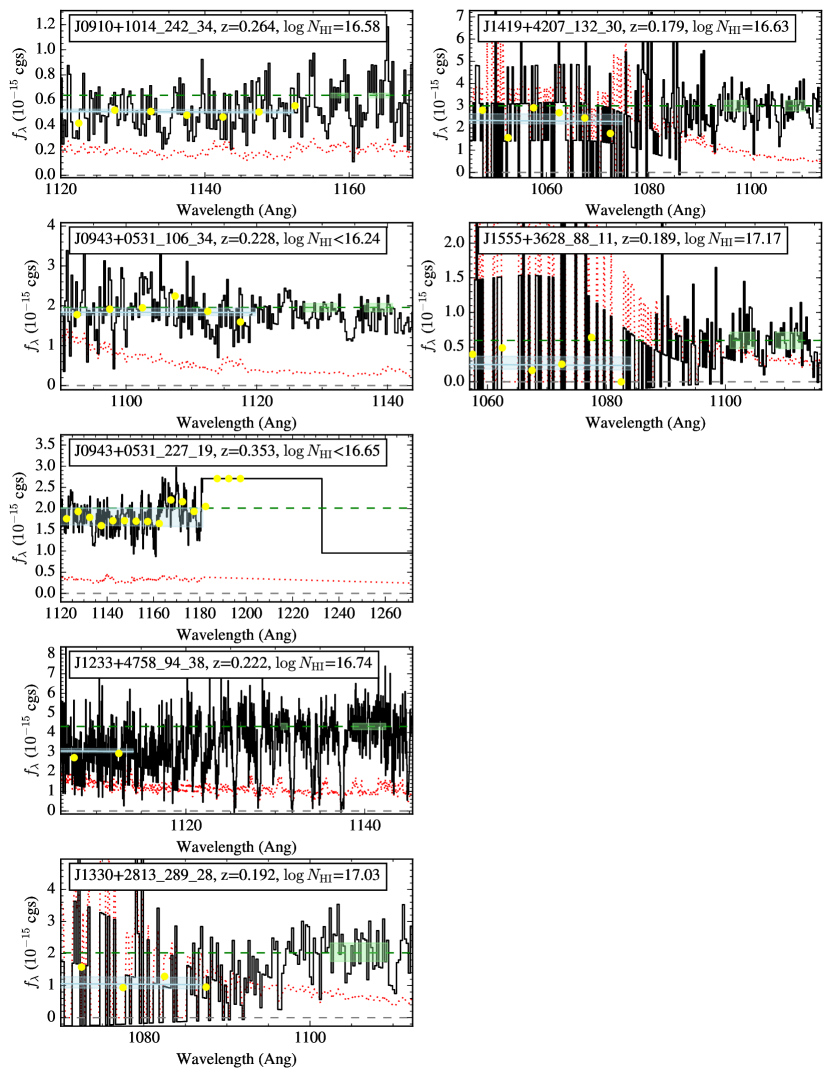
Figure 18: Same as Figure 1 but for the remainder of the sample.

Appendix B Ionization Modeling for Metallicity Evaluation

In W14, we constructed photo-ionization models for 29 sightlines in the COS-Halos sample. Following standard practice, we compared the ionic column densities $N_{\rm ion}$ integrated over the full system of low and intermediate ionization states (e.g., Si⁺, Si⁺⁺, Mg⁺) against a grid of photoionization models generated with the Cloudy software package (Ferland et al., 2013). Throughout the W14 analysis, we assumed the Haardt & Madau (2001) extragalactic UV background (EUVB; HM2001) radiation field and imposed the arbitrary prior that the gas metallicity could not exceed the solar value, which has been violated in several absorption systems in other studies (e.g. Tripp et al., 2011; Meiring et al., 2013). Constraints on the ionization model, specifically the ionization parameter $U$, were assessed primarily through a visual comparison of the data to models. Conservative estimates on the error in $U$ were adopted to account for this ‘by-eye’ procedure and the simplifying assumptions inherent to the photoionization modeling (e.g., a constant density gas).

There are several differences between this analysis and W14. First, we have reassessed the measurements of ions in the COS spectra and redefined previously reported detections as upper limits or as non-constraining due to unidentified blends or poor data quality. Table 5 summarizes the modifications. Second, we have ignored Mg I throughout the analysis. We have found that ${N({\rm Mg^{0}})}$ rarely offers a meaningful constraint and in a few cases yields highly conflicting results (especially in systems with large $N_{\rm HI}$). Evidently our ionization models do not capture an aspect of the astrophysics (e.g., dust extinction, an unresolved colder phase) or atomic physics (e.g. recombination coefficients) relevant to Mg I. Third, we have modeled our spectra using the most recent EUVB from (Haardt & Madau, 2012, HM2012), which exhibits a shallower slope than HM2001 between 1.5 $-$ 4 Ryd. In other words, HM2001 somewhat under-produces species with ionization potential energies between 1.5 and 4 Ryd (e.g. SiIII) relative to the lower ionization potential ions (e.g. MgII, SiII) compared to HM2012. Overall, the difference is such that the gas ionization parameters derived from HM2001 will be $\sim$0.3 dex higher than those derived from HM2012 for the same sightlines.

Table 5: COLUMN DENSITY UPDATES

System	Ion/Transa	$f_{\rm orig}^{b}$	$f_{\rm new}^{b}$
J0910+1014_34_46	${\rm N}^{+}$	1	3
J0928+6025_110_35	FeIII 1122	2	1
J0943+0531_227_19	${\rm N}^{+}$	2	3
	${\rm C}^{+}$	1	3
J1016+4706_274_6	FeII 1144	1	3
J1342-0053_157_10	OI 971	1	3
J1435+3604_68_12	OI 971	1	3
J1619+3342_113_40	${\rm C}^{+}$	1	3
J2345-0059_356_12	NII 1083	1	3
	SiIII 1206	1	0

Fourth, and most importantly, we adopt a Monte Carlo Markov Chain (MCMC) approach to compare an interpolated photoionization grid to the observational constraints from each system. Full details of the procedure are provided in Fumagalli et al. (2016) and the code is publicly available and makes use of the EMCEE package (Foreman-Mackey et al., 2013). Here we briefly summarize the algorithm. We first generated a grid of equilibrium photoionization models (recovering $T\sim 10^{4}$ K), each with a constant gas density $n_{\rm H}$. The gas has solar relative abundances (Asplund et al., 2009), scaled to a global metallicity [Z/H]. The grid has two additional parameters: the integrated H I column density $N_{\rm HI}$ and the redshift $z$. The latter sets the adopted radiation field which is taken to be the extragalactic UV background (EUVB) derived from the CUBA package (Haardt & Madau, 2012). The uncertainty in the EUVB intensity remains large (e.g. Kollmeier et al., 2014) and this primarily affects our density estimations. Systematic uncertainty in the shape of the EUVB imposes a systematic error in the metallicity of $\approx 0.3$ dex (Howk et al., 2009; Fumagalli et al., 2016; Wotta et al., 2016). The $N_{\rm HI}$ value sets the thickness of the plane parallel gas layers for each solution The ranges for the four grid parameters are summarized in Table 6. For the two systems analyzed with $\log N_{\rm HI}<15$, we ran the analysis assuming $\log N_{\rm HI}=15.5$ and afterwards offset accordingly the outputs. At these low $N_{\rm HI}$ values where the gas is optically thin to ionizing radiation, the relative populations of the ionization states have very little $N_{\rm HI}$ dependence.

Table 6: Cloudy Model Parameters

Parameter	Range	Step Size
[Z/H]	-4, 2.5	0.25
z	0, 4.5	0.25
$\log N_{\rm HI}/\,{\rm cm^{-2}}$	15, 20.5	0.25
$\log n_{\rm H}/\,{\rm cm^{-3}}$	-4.5, 0	0.25

We emphasize that the models assume an overly simplified constant density for all gas layers. Recent work has demonstrated that relaxing this assumption may describe a wider range of the observed ions with even fewer parameters (Stern et al., 2016). On the other hand, we are strongly motivated to these ‘single phase’ models by the tight kinematic correspondence between the H I Lyman series and the lower ionization state gas (Werk et al., 2016) and because these models provide a good fit to the lower ionization state gas in the majority of cases (see also Haislmaier et al., In prep).

For each CGM system, we performed an initial run with the MCMC randomly seeding the initial values for the walkers throughout the full grid of model parameter space. We generated 960 walkers with 480 samples per MCMC chain (eventually removing a ‘burn-in’ set of 45 samples per chain). For those systems with at least one measurement of an ion column density, the acceptance rate was approximately a nominal level of 0.5. The 9 systems without a metal constraint yielded a zero acceptance rate and are considered no further.

We then performed a second MCMC run seeded by the initial results. We initialized these chains at the median values of the initial runs with a normal deviate in log10 space of 0.01 dex. From this second run, we derive the final adopted probability distribution functions (PDFs) for the model parameters.

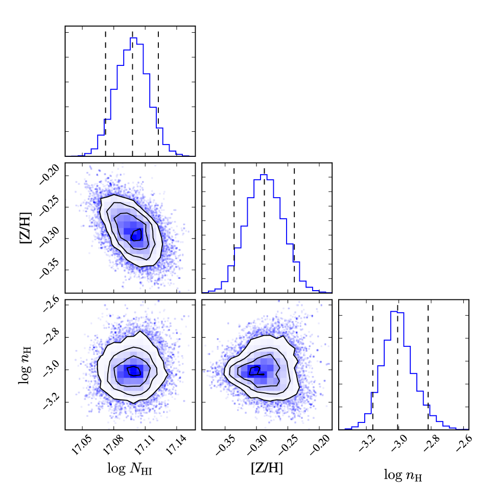
Figure 19: A ‘corner’ plot of the MCMC PDF for the model parameters of J1016+4706_274_6. This describes the distribution of model parameters in the MCMC chains.

Figure 19 shows a corner plot for three of the model parameters for a well-constrained system (J1016+4706_274_6). We designate the preferred or ‘best’ model from the median of the parameter PDFs when discussing individual systems and the uncertainties are based on percentiles of the PDF. These quantities are well-behaved for this model. Figure 20 compares the observational constraints with the model PDFs for the ionic column densities. All of the observables are well-modeled with a slight tension for S III and the under-prediction of Mg II. Such deviations from these species are common in absorption-line modeling (e.g. Prochaska, 1999; Crighton et al., 2015; Haislmaier et al., In prep; Wotta et al., 2016), and they suggest either over-simplifications in the modeling (e.g. constant density), non-solar relative abundances within the gas from nucleosynthesis, and/or differential dust depletion. For completeness, Table 7 provides the measurements of each ionic column density used in the analysis and the model results.

Table 7: IONIC COLUMN DENSITIES AND MODEL VALUES

Galaxy	Ion	$\log N$	$\sigma(\log N)^{a}$	Modelb
J0401-0540_67_24	OI	14.15	99	9.77,11.92
	SiII	12.47	99	11.56,13.14
	CII	13.58	99	12.99,13.77
	MgII	12.26	99	10.87,12.39
	NII	13.55	99	12.16,13.12
	FeII	13.89	99	9.24,11.77
	FeIII	13.85	99	11.63,12.79
	SiIII	12.88	0.06	12.77,13.00
	CIII	14.00	-1	14.01,14.94
J0803+4332_306_20	OI	14.17	99	7.21,14.86
	SiII	12.68	99	9.58,13.82
	CII	13.58	99	11.89,14.65
	MgII	12.00	99	7.99,13.86
	NII	13.68	99	10.79,13.86
	FeII	13.58	99	6.36,13.79
	FeIII	14.16	99	9.32,12.70
	SiIII	12.48	99	10.86,12.66
	CIII	13.67	0.06	13.54,13.78

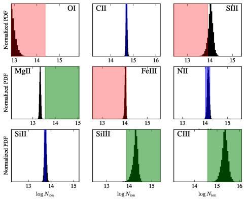
Figure 20: Each panel compares the model predictions for the ionic column densities $N_{\rm ion}$ against the observational constraints (ordered by ionization potential). Blue shaded regions indicate a measured value for $N_{\rm ion}$ with $1\sigma$ uncertainty whereas the pink/green regions indicate upper/lower limits on $N_{\rm ion}$ respectively. With the exception of Mg II, where the model under-predicts the observed constraint, there is good agreement.

For comparison with other results from photoionization modeling of absorption systems, we estimate $\log U\approx-3.1$ for $\log n_{\rm H}=-3$ at $z=0.2$ for our adopted EUVB where $U\equiv\Phi/(cn_{\rm H}$ with $\Phi$ the flux of ionizing photons. If one were to increase/decrease the intensity, e.g. a local enhancement related to star-formation within the galaxy, the first-order effect is a corresponding increase/decrease in $n_{\rm H}$ because the relative ionic column densities are most sensitive to $U$.

Figure 21 shows another corner plot for one of the MCMC models. In contrast to Figure 19, this model has fewer observational detections and the resultant constraints on the model are poorer.

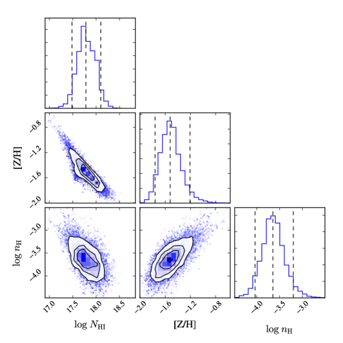
Figure 21: Same as Figure 19 but for a system with fewer observational constraints.

The MCMC analysis yields metallicity PDFs for cool CGM gas under the assumption of photoionization equilibrium. Figure 22 shows four PDFs for systems with a varying set of observational constraints. The top system (J0226+0015_268_22) has no positive detections of any metal transition and therefore no meaningful constraint on the PDF.

The second example (J0401$-$0540_67_24 with $N_{\rm HI}=10^{15.45}\,{\rm cm^{-2}}$) shows only a single ${N({\rm\rm Si^{++}})}$ detection and several upper limits from non-detections. The metallicity PDF is driven to high values because there is a maximal Si⁺⁺/H⁰ ratio for photoionization models which establishes a lower limit to the gas metallicity. The final two examples in Figure 22 are systems with a large set of ion constraints. One system J1016+4706_359_16 has an imprecise $N_{\rm HI}$ measurement and a correspondingly large uncertainty on [Z/H]. The other, J1419+4207_132_30, shows that metallicities can be estimated to $\pm 0.2$ dex in the best circumstances.

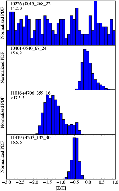
Figure 22: Derived metallicity PDFs for four representative CGM systems from the COS-Halos sample. The top panel shows an example without a constraint on any heavy element. The second system (J0401-0540_67_24) exhibits a positive detection of Si⁺⁺ and a low $N_{\rm HI}$ value which drives the solution to a high [Z/H] value. The last two systems exhibit many ionic transitions. The relatively large uncertainty in [Z/H] for J1016+4706_359_16 reflects the large uncertainty in $N_{\rm HI}$ for this system owing to a fully saturated Lyman limit. Labels under each system name give the $\log N_{\rm HI}$ value followed by the number of positive detections used to constrain the metallicity PDF.

Appendix C Ionization corrections for Super-solar Gas

In Section 4.3 we reported on several CGM systems with estimated metallicities of solar or even super-solar abundances. These results were derived from our MCMC analysis of the H I column density and the observed set of metals. Qualitatively, however, the requirement of a high metallicity may be inferred simply from the single observational constraint on the ratio of ${N({\rm Si^{++}})}$ to $N_{\rm HI}$.

Figure 23 presents the combined ionization and abundance corrections required to convert an observed $\log[{N({\rm Si^{++}})}/N_{\rm HI}]$ measurement to an estimate of [Si/H] value. The ionization corrections assume photoionization equilibrium and a gas with solar metallicity (adopting a lower metallicity would imply a small difference in the calculation). Examining the figure, one notes that the smallest correction is $\approx 2.4$ dex and occurs for gas with low $N_{\rm HI}$ and low density (i.e. a high ionization parameter). Therefore, under the assumption of photoionization equilibrum (the results are similar for collisional ionization), any system exhibiting $\log[{N({\rm Si^{++}})}-N_{\rm HI}]>-2.4$ dex indicates at least a solar abundance of Si.

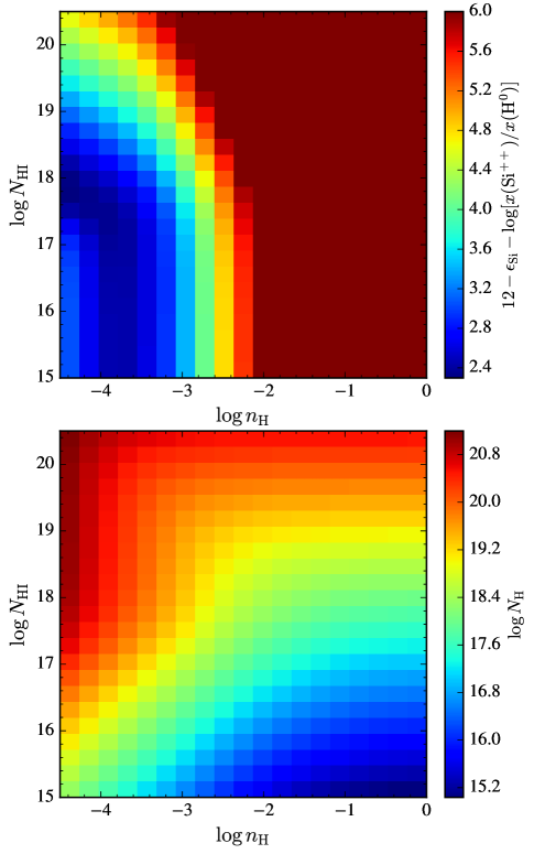
Figure 23: (top) Correction that must be applied to convert an observed $\log[{N({\rm Si^{++}})}/N_{\rm HI}]$ measurement to an estimate of [Si/H] value for photoionization models with the range of $N_{\rm HI}$ and $\log n_{\rm H}$ values indicated. The minimum correction is $2.4$ dex and this sets a conservative lower limit to [Si/H] for a set of systems in the COS-Halos sample. (bottom) Derived total hydrogen column density $N_{\rm H}$ for the same models.

References

- Anderson & Bregman (2010) Anderson, M. E., & Bregman, J. N. 2010, ApJ, 714, 320
- Asplund et al. (2009) Asplund, M., Grevesse, N., Sauval, A. J., & Scott, P. 2009, ARA&A, 47, 481
- Bahcall & Spitzer (1969) Bahcall, J. N., & Spitzer, L. J. 1969, ApJ, 156, L63
- Battisti et al. (2012) Battisti, A. J., Meiring, J. D., Tripp, T. M., et al. 2012, ApJ, 744, 93
- Bergeron (1986) Bergeron, J. 1986, A&A, 155, L8
- Bland-Hawthorn & Maloney (2001) Bland-Hawthorn, J., & Maloney, P. R. 2001, ApJ, 550, L231
- Bordoloi et al. (2014) Bordoloi, R., Tumlinson, J., Werk, J. K., et al. 2014, ApJ, 796, 136
- Borthakur et al. (2014) Borthakur, S., Heckman, T. M., Leitherer, C., & Overzier, R. A. 2014, Science, 346, 216
- Borthakur et al. (2015) Borthakur, S., Heckman, T., Tumlinson, J., et al. 2015, ApJ, 813, 46
- Bowen et al. (2016) Bowen, D. V., Chelouche, D., Jenkins, E. B., et al. 2016, ApJ, 826, 50
- Boylan-Kolchin et al. (2013) Boylan-Kolchin, M., Bullock, J. S., Sohn, S. T., Besla, G., & van der Marel, R. P. 2013, ApJ, 768, 140
- Burchett et al. (2016) Burchett, J. N., Tripp, T. M., Bordoloi, R., et al. 2016, ApJ, 832, 124
- Cantalupo (2010) Cantalupo, S. 2010, MNRAS, 403, L16
- Chen et al. (2001) Chen, H.-W., Lanzetta, K. M., & Webb, J. K. 2001, ApJ, 556, 158
- Collins et al. (2007) Collins, J. A., Shull, J. M., & Giroux, M. L. 2007, ApJ, 657, 271
- Cooksey et al. (2010) Cooksey, K. L., Thom, C., Prochaska, J. X., & Chen, H. 2010, ApJ, 708, 868
- Crighton et al. (2015) Crighton, N. H. M., Hennawi, J. F., Simcoe, R. A., et al. 2015, MNRAS, 446, 18
- Davé & Oppenheimer (2007) Davé, R., & Oppenheimer, B. D. 2007, MNRAS, 374, 427
- Faerman et al. (2017) Faerman, Y., Sternberg, A., & McKee, C. F. 2017, ApJ, 835, 52
- Fang et al. (2013) Fang, T., Bullock, J., & Boylan-Kolchin, M. 2013, ApJ, 762, 20
- Fang et al. (2015) Fang, T., Buote, D., Bullock, J., & Ma, R. 2015, ApJS, 217, 21
- Fang et al. (2006) Fang, T., Mckee, C. F., Canizares, C. R., & Wolfire, M. 2006, ApJ, 644, 174
- Feigelson & Nelson (1985) Feigelson, E. D., & Nelson, P. I. 1985, ApJ, 293, 192
- Ferland et al. (2013) Ferland, G. J., Porter, R. L., van Hoof, P. A. M., et al. 2013, Rev. Mexicana Astron. Astrofis., 49, 137
- Ford et al. (2014) Ford, A. B., Davé, R., Oppenheimer, B. D., et al. 2014, MNRAS, 444, 1260
- Foreman-Mackey et al. (2013) Foreman-Mackey, D., Hogg, D. W., Lang, D., & Goodman, J. 2013, PASP, 125, 306
- Fox et al. (2006) Fox, A. J., Savage, B. D., & Wakker, B. P. 2006, ApJS, 165, 229
- Fukugita et al. (1998) Fukugita, M., Hogan, C. J., & Peebles, P. J. E. 1998, ApJ, 503, 518
- Fumagalli et al. (2016) Fumagalli, M., O’Meara, J. M., & Prochaska, J. X. 2016, MNRAS, 455, 4100
- Gibson et al. (2001) Gibson, B. K., Giroux, M. L., Penton, S. V., et al. 2001, AJ, 122, 3280
- Gnat & Sternberg (2007) Gnat, O., & Sternberg, A. 2007, ApJS, 168, 213
- Greco et al. (2015) Greco, J. P., Hill, J. C., Spergel, D. N., & Battaglia, N. 2015, ApJ, 808, 151
- Gupta et al. (2012) Gupta, A., Mathur, S., Krongold, Y., Nicastro, F., & Galeazzi, M. 2012, ApJ, 756, L8
- Haardt & Madau (2001) Haardt, F., & Madau, P. 2001, in Clusters of Galaxies and the High Redshift Universe Observed in X-rays, ed. D. M. Neumann & J. T. V. Tran
- Haardt & Madau (2012) Haardt, F., & Madau, P. 2012, ApJ, 746, 125
- Hafen et al. (2016) Hafen, Z., Faucher-Giguere, C.-A., Angles-Alcazar, D., et al. 2016, ArXiv e-prints, arXiv:1608.05712
- Haislmaier et al. (In prep) Haislmaier, K., , & . In prep, ApJ
- Hinshaw et al. (2013) Hinshaw, G., Larson, D., Komatsu, E., et al. 2013, ApJS, 208, 19
- Howk et al. (2009) Howk, J. C., Ribaudo, J. S., Lehner, N., Prochaska, J. X., & Chen, H. 2009, MNRAS, 396, 1875
- Izotov et al. (2016) Izotov, Y. I., Schaerer, D., Thuan, T. X., et al. 2016, MNRAS, 461, 3683
- Johnson et al. (2015) Johnson, S. D., Chen, H.-W., & Mulchaey, J. S. 2015, MNRAS, 449, 3263
- Klypin et al. (2002) Klypin, A., Zhao, H., & Somerville, R. S. 2002, ApJ, 573, 597
- Kollmeier et al. (2014) Kollmeier, J. A., Weinberg, D. H., Oppenheimer, B. D., et al. 2014, ApJ, 789, L32
- Lau et al. (2016) Lau, M. W., Prochaska, J. X., & Hennawi, J. F. 2016, ApJS, 226, 25
- Lehner et al. (2015) Lehner, N., Howk, J. C., & Wakker, B. P. 2015, ApJ, 804, 79
- Lehner et al. (2014) Lehner, N., O’Meara, J. M., Fox, A. J., et al. 2014, ApJ, 788, 119
- Lehner et al. (2013) Lehner, N., Howk, J. C., Tripp, T. M., et al. 2013, ApJ, 770, 138
- Leitherer et al. (1995) Leitherer, C., Ferguson, H. C., Heckman, T. M., & Lowenthal, J. D. 1995, ApJ, 454, L19
- Leitherer et al. (2016) Leitherer, C., Hernandez, S., Lee, J. C., & Oey, M. S. 2016, ApJ, 823, 64
- Loveday et al. (2015) Loveday, J., Norberg, P., Baldry, I. K., et al. 2015, MNRAS, 451, 1540
- Matteucci & Gibson (1995) Matteucci, F., & Gibson, B. K. 1995, A&A, 304, 11
- Maughan et al. (2008) Maughan, B. J., Jones, C., Forman, W., & Van Speybroeck, L. 2008, ApJS, 174, 117
- Meiring et al. (2013) Meiring, J. D., Tripp, T. M., Werk, J. K., et al. 2013, ApJ, 767, 49
- Nicastro et al. (2016) Nicastro, F., Senatore, F., Gupta, A., et al. 2016, MNRAS, 458, L123
- Oppenheimer & Schaye (2013) Oppenheimer, B. D., & Schaye, J. 2013, MNRAS, 434, 1063
- Oppenheimer et al. (2016) Oppenheimer, B. D., Crain, R. A., Schaye, J., et al. 2016, MNRAS, 460, 2157
- Peeples & Shankar (2011) Peeples, M. S., & Shankar, F. 2011, MNRAS, 417, 2962
- Peeples et al. (2014) Peeples, M. S., Werk, J. K., Tumlinson, J., et al. 2014, ApJ, 786, 54
- Planck Collaboration et al. (2013) Planck Collaboration, Ade, P. A. R., Aghanim, N., et al. 2013, A&A, 557, A52
- Prochaska (1999) Prochaska, J. X. 1999, ApJ, 511, L71
- Prochaska et al. (2013) Prochaska, J. X., Hennawi, J. F., & Simcoe, R. A. 2013, ApJ, 762, L19 (QPQ5)
- Prochaska et al. (2011) Prochaska, J. X., Weiner, B., Chen, H.-W., Mulchaey, J., & Cooksey, K. 2011, ApJ, 740, 91
- Prochaska et al. (2006) Prochaska, J. X., Weiner, B. J., Chen, H.-W., & Mulchaey, J. S. 2006, ApJ, 643, 680
- Putman et al. (2012) Putman, M. E., Peek, J. E. G., & Joung, M. R. 2012, ARA&A, 50, 491
- Rasmussen & Ponman (2009) Rasmussen, J., & Ponman, T. J. 2009, MNRAS, 399, 239
- Ribaudo et al. (2011a) Ribaudo, J., Lehner, N., & Howk, J. C. 2011a, ApJ, 736, 42
- Ribaudo et al. (2011b) Ribaudo, J., Lehner, N., Howk, J. C., et al. 2011b, ApJ, 743, 207
- Schaye et al. (2007) Schaye, J., Carswell, R. F., & Kim, T.-S. 2007, MNRAS, 379, 1169
- Sembach et al. (2006) Sembach, K. R., Wakker, B. P., Savage, B. D., & Richter, P. 2006, in Astronomical Society of the Pacific Conference Series, Vol. 348, Astrophysics in the Far Ultraviolet: Five Years of Discovery with FUSE, ed. G. Sonneborn, H. W. Moos, & B.-G. Andersson, 375
- Shen et al. (2013) Shen, S., Madau, P., Guedes, J., et al. 2013, ApJ, 765, 89
- Shull et al. (2010) Shull, J. M., France, K., Danforth, C. W., Smith, B., & Tumlinson, J. 2010, ApJ, 722, 1312
- Sivanandam et al. (2009) Sivanandam, S., Zabludoff, A. I., Zaritsky, D., Gonzalez, A. H., & Kelson, D. D. 2009, ApJ, 691, 1787
- Stern et al. (2016) Stern, J., Hennawi, J. F., Prochaska, J. X., & Werk, J. K. 2016, ApJ, 830, 87
- Stinson et al. (2012) Stinson, G. S., Brook, C., Prochaska, J. X., et al. 2012, MNRAS, 425, 1270
- Stocke et al. (2013) Stocke, J. T., Keeney, B. A., Danforth, C. W., et al. 2013, ApJ, 763, 148
- Sunyaev & Zeldovich (1972) Sunyaev, R. A., & Zeldovich, Y. B. 1972, Comments on Astrophysics and Space Physics, 4, 173
- Syphers & Shull (2014) Syphers, D., & Shull, J. M. 2014, ApJ, 784, 42
- Thom et al. (2008) Thom, C., Peek, J. E. G., Putman, M. E., et al. 2008, ApJ, 684, 364
- Tripp et al. (2000) Tripp, T. M., Savage, B. D., & Jenkins, E. B. 2000, ApJ, 534, L1
- Tripp et al. (2011) Tripp, T. M., Meiring, J. D., Prochaska, J. X., et al. 2011, Science, 334, 952
- Tumlinson et al. (2011) Tumlinson, J., Thom, C., Werk, J. K., et al. 2011, Science, 334, 948
- Tumlinson et al. (2013) —. 2013, ApJ, 777, 59
- Turner et al. (2014) Turner, M. L., Schaye, J., Steidel, C. C., Rudie, G. C., & Strom, A. L. 2014, MNRAS, 445, 794
- Veilleux et al. (2005) Veilleux, S., Cecil, G., & Bland-Hawthorn, J. 2005, ARA&A, 43, 769
- Verner et al. (1996) Verner, D. A., Ferland, G. J., Korista, K. T., & Yakovlev, D. G. 1996, ApJ, 465, 487
- Wakker (2015) Wakker, B. P. 2015, Highlights of Astronomy, 16, 598
- Wakker et al. (2008) Wakker, B. P., York, D. G., Wilhelm, R., et al. 2008, ApJ, 672, 298
- Weiner et al. (2001) Weiner, B. J., Vogel, S. N., & Williams, T. B. 2001, in Astronomical Society of the Pacific Conference Series, Vol. 240, Gas and Galaxy Evolution, ed. J. E. Hibbard, M. Rupen, & J. H. van Gorkom, 515
- Werk et al. (2012) Werk, J. K., Prochaska, J. X., Thom, C., et al. 2012, ApJS, 198, 3
- Werk et al. (2014) Werk, J. K., Prochaska, J. X., Tumlinson, J., et al. 2014, ApJ, 792, 8
- Werk et al. (2016) Werk, J. K., Prochaska, J. X., Cantalupo, S., et al. 2016, ApJ, 833, 54
- Worseck et al. (2016) Worseck, G., Prochaska, J. X., Hennawi, J. F., & McQuinn, M. 2016, ApJ, 825, 144
- Wotta et al. (2016) Wotta, C. B., Lehner, N., Howk, J. C., O’Meara, J. M., & Prochaska, J. X. 2016, ApJ, 831, 95
- Yao & Wang (2007) Yao, Y., & Wang, Q. D. 2007, ApJ, 658, 1088
- Zheng et al. (2015) Zheng, Y., Putman, M. E., Peek, J. E. G., & Joung, M. R. 2015, ApJ, 807, 103
- Zhu et al. (2014) Zhu, G., Ménard, B., Bizyaev, D., et al. 2014, MNRAS, 439, 3139