Atmospheric Trident Production for Probing New Physics

Abstract

We propose to use atmospheric neutrinos as a powerful probe of new physics beyond the Standard Model via neutrino trident production. The final state with double muon tracks simultaneously produced from the same vertex is a distinctive signal at large Cherenkov detectors. We calculate the expected event numbers of trident production in the Standard Model. To illustrate the potential of this process to probe new physics we obtain the sensitivity on new vector/scalar bosons with coupling to muon and tau neutrinos.

Introduction – The neutrino oscillation is the first place that new physics (NP) beyond the Standard Model (SM) was observed sk . In less than two decades, a consistent minimal picture has emerged: three flavor states whose mixing with each other is described by a unitary matrix, together with interactions predicted by the SM nuRev . However, neutrino oscillation cannot directly test the underlying picture behind the neutrino mass and mixing. We need new concept to go beyond.

The rare process of neutrino trident production trident ; coherent ,

$$\stackrel{{\scriptstyle(-)}}{{\nu_{\ell}}}N\to\stackrel{{\scriptstyle(-)}}{{\nu_{\ell}}}\ell^{+}\ell^{-}X\mbox{ with }\ell=e,\mu,\tau\,,$$ (1)

can serve the purpose of directly probing the underlying principle of neutrino physics. While neutrino oscillation experiment focuses on reconstructing the initial state, namely the incident neutrino energy and flavor, neutrino trident production can produce new particles as intermediate state (see Fig. 1) and constrain their properties by observing the final-state particles. Essentially, we can turn an oscillation experiment into a “neutrino collider”.

Neutrino Trident Production in the Standard Model – In neutrino trident production, three leptonic particles appear in the final state. One is a neutrino and the other two a pair of leptons with opposite charge,

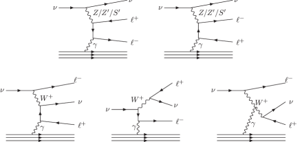
Figure 1: Feynman diagrams for neutrino trident production in the SM and in the presence of a vector (scalar) boson $Z^{\prime}$ ($S^{\prime}$).

as plotted in Fig. 1.

At leading order, the leptonic part connects with nuclei through a photon. The $Z$ boson can also establish the connection but its contribution is highly suppressed by its heavy propagators. Suppression also occurs in the last diagram in Fig. 1 through two $W$ propagators. Since the connection with nuclei is established by a photon, which is electrically neutral, there is no difference between the neutrino and anti-neutrino modes, i.e. $\sigma_{\nu}(E)=\sigma_{\bar{\nu}}(E)$. However, the differential distributions of the two final-state charged leptons have some measurable difference if charge identification is possible. Because of the $W$ contribution, there is no interchange symmetry between the two charged leptons. Since the connection with the nucleus is established through a photon, this process actually probes the electromagnetic structure Gao:2003ag of the target nuclei with suppressed momentum transfer. We implement the form factors for coherent coherent and diffractive diffractive regions in CompHEP CompHEP to simulate the $\nu N\rightarrow\nu\ell^{+}\ell^{-}N$ process with four-body final state.

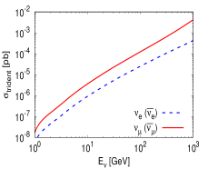
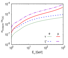
Figure 2: The SM prediction of the neutrino trident production cross section on water target (left) and its relative value with respect to the cross section of CC scattering (right).

The energy dependence of the trident production cross section $\sigma_{\rm trident}$ is shown in Fig. 2. Below 2 GeV, $\sigma_{\rm trident}$ increases quickly after the channel opens up at the muon pair production threshold $E^{\rm th}_{\nu}=2m_{\mu}\simeq 210\,\mbox{MeV}$. For comparison, the cross section $\sigma_{\rm CC}$ of the charged-current (CC) scattering of neutrinos on the same water target is simulated with GENIE GENIE . As shown in the right panel of Fig. 2, the cross section of neutrino trident production is roughly $4\sim 6$ orders smaller than the one of neutrino scattering in the range $E_{\nu}\gtrsim 2\,\mbox{GeV}$. The higher the neutrino energy, the larger $\sigma_{\rm trident}$ and $\sigma_{\rm trident}/\sigma_{\rm CC}$.

Neutrino Trident Observation at Cherenkov Detectors – To collect a handful of neutrino trident events, the same experiment should be able to collect at least $\mathcal{O}(10^{6})$ of the ordinary neutrino CC events which is a quite large event number for the existing and next-generation neutrino experiments. Regarding man-made neutrino sources, the only possibility is provided by accelerator experiments Altmannshofer:2014pba , including the past experiments CHARM-II CHARM2 , CCFR CCFR and NuTeV NuTeV , as well as the future high-intensity neutrino facilities such has DUNE Magill:2016hgc . Here we propose using the free source of atmospheric neutrinos to observe neutrino trident production at large Cherenkov detectors, such as PINGU PINGU and ORCA KM3net .

These Cherenkov detectors are huge ice/water cubes filled with vertical strings of digital optical modules (DOMs). The ice/water is used both as scattering target and measurement medium. Charged particles traveling faster than the speed of light in ice/water, which is roughly $3/4$ of the speed of light in vacuum, produce Cherenkov radiation and the DOMs record the energy and arriving time of Cherenkov photons to reconstruct the momentum and flavor of the charged particles. Especially muons can leave a clear track inside the detector while electrons leave more spherical radiation. This difference can be used to identify muons effectively.

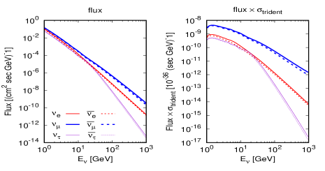
Figure 3: Atmospheric neutrino fluxes at South Pole Honda after oscillation. The Mediterranean sites have similar fluxes.

The original atmospheric neutrino flux Honda needs to be folded with neutrino oscillation probabilities, which depend on both oscillation parameters and the Earth matter density. A numerical evaluation of neutrino oscillations with decomposition in the propagation basis and applying the PREM Earth matter profile PREM can be found in atmos and has been implemented in the NuPro package nupro . For simplicity, we take the current global best fit-values global of neutrino oscillation parameters to calculate the fluxes arriving at Cherenkov detectors, as shown in Fig. 3.

For a neutrino telescope that cannot distinguish muon charge, such as PINGU and ORCA, a huge detector size is necessary for the mass hierarchy measurement. Its effective volume can be as large as $5$ Mt (PINGU PINGU ) and $6$ Mt (ORCA KM3net ) at $E_{\nu}\sim 30\mbox{\,GeV}$. Every year, PINGU can collect $1.6\times 10^{5}$ events Cowen . For a period of 6 years, one million events can be collected. This is roughly what we need to collect around 10 events of neutrino trident production. The same observation can also happen at the larger versions, IceCube ($\sim 200\,\mbox{Mt}$) IceCube , DeepCore ($\sim 60\,\mbox{Mt}$) DeepCore , and ARCA ($\sim 300\,\mbox{Mt}$) KM3net at $E_{\nu}=500\,\mbox{GeV}$.

By folding the cross section of neutrino trident production with the atmospheric neutrino flux after propagating through the Earth, and taking into account the effective volume, we calculate the SM prediction for the neutrino trident event rate and display it in Fig. 4 for both neutrinos and anti-neutrinos. Different from the ordinary scattering process, the event rate of neutrino trident production keeps growing until $E_{\nu}\sim 10\,\mbox{GeV}$.

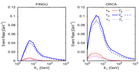
Figure 4: The SM prediction of the neutrino trident production event rate at PINGU (left) and ORCA (right).

The total rate is 7.4 (17, 63) and 16 (23) events for 10 years running of PINGU (DeepCore, IceCube) and ORCA (ARCA). The South Pole (Mediterranean) combination can collect 87 (39) events and statistically the uncertainty can be as small as $11\%$ ($16\%$). Of course, there are systematical uncertainties, such as the normalization of the predicted atmospheric neutrino flux which can be as large as 20% Honda . Fortunately, the ordinary neutrino scattering process can collect millions of events to constrain the normalization with unprecedented sub-percent precision.

Coincident muon tracks can fake the muon pair from neutrino trident production. However, the cosmic muons can be vetoed by the detectors outside or on the surface for PINGU, or in case of ORCA with dedicated kinematic cuts. The irreducible background comes from the yearly $N_{\mu}\equiv 8.6\times 10^{4}$ CC muon events (at PINGU). By applying coincidence cuts, namely requiring the two muons to appear simultaneously within a narrow time window $\Delta t$, the fake rate can be suppressed to $C_{N_{\mu}}^{2}\times(\Delta t/T)^{2}$, where $T=3.15\times 10^{7}$ is the length of a year and $C_{N_{\mu}}^{2}=N_{\mu}(N_{\mu}-1)/2$ is the number of possible combinations with two out of the $N_{\mu}$ events to form a pair of muons as fake signal. Less than one background double-track requires $\Delta t\lesssim 500$ s, which is definitely achievable. In addition, the requirement that both muons come from the same vertex should further reduce the background rate. With increasing event number, the time window decreases as $\Delta t\propto 1/N_{\mu}$. So the same technique can also apply to DeepCore, IceCube, and ARCA.

Another possible background comes from the CC scattering with one primary muon and another faked muon from pion or charm decay. However, this background has totally different kinematics than the signal. While the background event is associated with hadronic shower to produce pion or charm, the signal has highly suppressed momentum transfer to the target nuclei due to the massless photon propagator and the electromagnetic form factor. In addition, the muon from pion or charm decay tends to have tiny energy. The signal has purely two energetic muons which is a very clear signal in Cherenkov detector.

All these points are beneficial for the observation of neutrino trident production at large Cherenkov detectors. First, the large detector size ensures enough event rate. Second, the double-track signal is easy to identify double-track without modification of the detector and the search can be carried out simultaneously with the neutrino oscillation measurement. Finally, both systematics and background rate are small.

Neutrino Trident Production with New Physics – The effect of NP considered here appears by replacing the $Z$ boson with a new vector ($Z^{\prime}$) or scalar ($S^{\prime}$) boson. In principle all flavors contribute to Eq. (1). Here we focus on muon final states, because of strong constraints on new physics in the electron sector and because muons are easier to identify than other flavors.

For illustration of the vector boson case, we consider the $L_{\mu}-L_{\tau}$ model Lmtmod which is anomaly free Lmt . The relevant Lagrangian is

$$\mathcal{L}_{Z^{\prime}}\equiv g_{Z^{\prime}}Q_{\alpha\beta}\left[\overline{L}_{\alpha}\gamma^{\mu}L_{\beta}+\overline{\ell}_{R\alpha}\gamma^{\mu}\ell_{R\beta}\right]Z^{\prime}_{\mu}+h.c.$$ (2)

where $L_{\alpha}$ denotes the left-handed lepton doublet and $\ell_{R}$ the right-handed lepton. The $Z^{\prime}$ couples to the muon and tau flavors with opposite charge, $Q_{\alpha\beta}=\mbox{diag}(0,1,-1)$, where $(\alpha,\beta)\equiv(e,\mu,\tau)$ denotes the three lepton flavors. Apart from the quantum number assignment, there are two new parameters, the $Z^{\prime}$ mass $M_{Z^{\prime}}$ and coupling constant $g_{Z^{\prime}}$. Trident production with gauged $L_{\mu}-L_{\tau}$ has been discussed for other types of experiments in Altmannshofer:2014pba ; Kaneta:2016uyt . We do not consider models in which there is additional coupling of the $Z^{\prime}$ to quarks Crivellin:2015mga . Although there are various constraints Altmannshofer:2014pba , viable parameter space of its mass and coupling still exists. In case of a scalar boson, we apply a similar Lagrangian,

$$\mathcal{L}_{S^{\prime}}\equiv g_{S^{\prime}}Q_{\alpha\beta}\left[\overline{\ell_{R\alpha}}\ell_{L\beta}+\overline{\nu^{c}_{L\alpha}}\nu_{L\beta}\right]S^{\prime}+h.c.$$ (3)

Here the neutrino Yukawa coupling with the scalar $S^{\prime}$ is of Majorana type, but the results do not depend on that. For comparison, we keep the same charge assignment $Q_{\alpha\beta}$ as the $Z^{\prime}$ case. The above two Lagrangians are implemented in CompHEP CompHEP .

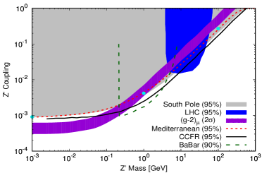
Figure 5: The sensitivity to the $Z^{\prime}$ mass and coupling at South Pole (PINGU+DeepCore+IceCube) Mediterranean (ORCA+ARCA), LHC Altmannshofer:2014pba , $(g-2)_{\mu}$ Altmannshofer:2014pba , CCFR Altmannshofer:2014pba , and BaBar BaBar experiments.

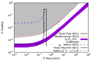
Figure 6: The sensitivity to the $S^{\prime}$ mass and coupling at South Pole (PINGU+DeepCore+IceCube), Mediterranean (ORCA+ARCA) and other experiments Batell:2016ove ; Pasquini:2015fjv .

We show the sensitivity to $M_{Z^{\prime}}$ and $g_{Z^{\prime}}$ in Fig. 5. Below $M_{Z^{\prime}}\sim 0.1\,\mbox{GeV}$, the curve is roughly flat while it grows fast for $M_{Z^{\prime}}\gg 0.1\,\mbox{GeV}$. This is because the $Z^{\prime}$ contribution contains a propagator $1/(q^{2}_{Z^{\prime}}-M^{2}_{Z^{\prime}})$, where $q_{Z^{\prime}}$ is the $t$-channel momentum transfer of $Z^{\prime}$. For light $Z^{\prime}$, $q^{2}_{Z^{\prime}}\gg M^{2}_{Z^{\prime}}$, the propagator is approximately $1/q^{2}_{Z^{\prime}}$, where $q_{Z^{\prime}}\gtrsim 1\,\mbox{GeV}$ is the typical momentum transfer, and hence insensitive to $M^{2}_{Z^{\prime}}$. On the other hand, for heavy $Z^{\prime}$, $q^{2}_{Z^{\prime}}\ll M^{2}_{Z^{\prime}}$, the propagator is roughly $1/M^{2}_{Z^{\prime}}$ and hence suppresses the rate with increasing $M_{Z^{\prime}}$. The same reasoning applies for $S^{\prime}$ as shown in Fig. 6. In both cases, the final sensitivities for the combinations PINGU+DeepCore and ORCA+ARCA are very similar in the plots.

For comparison, in Fig. 5 and Fig. 6 we also show constraints from other experiments. Although some of them are more stringent, such as $(g-2)_{\mu}$ measurement, they cannot directly confront and exclude the neutrino trident production. The interpretation of experimental data relies on theoretical assumption. The $(g-2)_{\mu}$ bound is based on the assumption that there is only $Z^{\prime}$ or $S^{\prime}$ contribution. Nevertheless, if there is something more that can also contribute to $(g-2)_{\mu}$ but not neutrino trident production, the $(g-2)_{\mu}$ constraint on $g_{Z^{\prime}/S^{\prime}}$ and $M_{Z^{\prime}/S^{\prime}}$ can be easily evaded. In addition, although the CCFR trident measurement $\sigma_{\rm CCFR}/\sigma_{\rm SM}=0.82\pm 0.28$, in contrast to the $11\%$ ($16\%$) at the South Pole (Mediterranean) combination, is claimed to give better sensitivity on $Z^{\prime}$, it might come from the fact that the central value deviates from the SM prediction.

In the current analysis we only use the total event number. There are several ways to further enhance the sensitivity. First, using differential distributions can significantly enhance the sensitivity of identifying NP from the SM, especially when the total cross section is comparable but differential distributions are different. We show the distributions of the opening angle $\theta_{\mu^{+}\mu^{-}}$ and energy sum $E_{\mu^{+}}+E_{\mu^{-}}$ the muon pair in Fig. 7 for illustration.

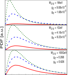
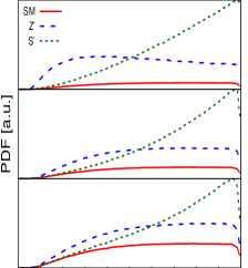
Figure 7: The distributions of the opening angle $\theta_{\mu^{+}\mu^{-}}$ (left) and total energy (right) of the muon pair produced in the neutrino trident production at oxygen nuclei.

Secondly, not just fully contained events can contribute. Those events being produced outside and going through or stop inside the detector can also be identified with two coincident tracks. Although not fully contained, the muon energy can be reconstructed according to the radiation pattern along the way, which is the so-called Edepillim Edepillim algorithm. The Edepillim algorithm can also identify overlapping double muon tracks. Finally, final-state leptons of not only muon flavor but also other combinations can be used to extract information on NP. With all improvements added, we can expect much better sensitivities from atmospheric neutrino experiments than the ones shown in Fig. 5 and Fig. 6.

Conclusion – We propose to use the free source of atmospheric neutrinos to probe neutrino physics, here in the form of vector and scalar bosons with coupling to muon neutrinos. The huge flux of atmospheric neutrinos and effective volume of large Cherenkov detectors are of great advantage to observe first the rare SM process of neutrino trident production, and also look for possible deviations arising from new physics. A pair of final-state muons can leave distinctive double tracks in the ice/water Cherenkov detector. Our analysis demonstrates that, in addition to pursuing their standard physics program, such experiments can make very useful contributions in constraining new physics without changing their configuration. This essentially turns neutrino telescope into neutrino collider. The original scripts for running CompHEP in batch mode can be downloaded from the NuTrident_CompHEP project at GitLab.

Acknowledgements – SFG would like to thank Wolfgang Altmannshofer, Vedran Brdar, Jürgen Brunner, Romulus Godang, Francis Halzen, Jannik Hofestädt, Morihiro Honda, Clancy James, David McKeen, Antoine David Kouchner, Pedro Pasquini, Sally Robertson, Carsten Rott for useful discussions and kind help. WR thanks Julian Heeck for helpful comments. This work was supported by the DFG with grant RO 2516/6-1 in the Heisenberg Programme (WR).

References

- (1) Y. Fukuda et al. [Super-Kamiokande Collaboration], Phys. Rev. Lett. 81, 1562 (1998) [arXiv:hep-ex/9807003].
- (2) R. N. Mohapatra et al., Rept. Prog. Phys. 70, 1757 (2007) [arXiv:hep-ph/0510213].
- (3) W. Czyz, G. C. Sheppey and J. D. Walecka, Nuovo Cim. 34, 404 (1964); K. Fujikawa, Annals Phys. 68, 102 (1971); K. Koike, M. Konuma, K. Kurata and K. Sugano, Prog. Theor. Phys. 46, 1150 (1971); K. Koike, M. Konuma, K. Kurata and K. Sugano, Prog. Theor. Phys. 46, 1799 (1971); R. W. Brown, R. H. Hobbs, J. Smith and N. Stanko, Phys. Rev. D 6, 3273 (1972); K. Fujikawa, Annals Phys. 75, 491 (1973); W. Jager, Nucl. Phys. B 142, 273 (1978); R. Belusevic and J. Smith, Phys. Rev. D 37, 2419 (1988); L. M. Sehgal, Phys. Rev. D 38, 2750 (1988); A. V. Kuznetsov, N. V. Mikheev and D. A. Rumyantsev, Phys. Atom. Nucl. 65, 277 (2002) [Yad. Fiz. 65, 303 (2002)]; M. I. Vysotsky, I. V. Gaidaenko and V. A. Novikov, Phys. Atom. Nucl. 65, 1634 (2002) [Yad. Fiz. 65, 1676 (2002)]; T. Jacobsen, [arXiv:hep-ph/0608150].
- (4) J. Lovseth and M. Radomiski, Phys. Rev. D 3, 2686 (1971);
- (5) H. Y. Gao, Int. J. Mod. Phys. E 12, 1 (2003) [Int. J. Mod. Phys. E 12, 567 (2003)] [arXiv:nucl-ex/0301002].
- (6) R. W. Brown, R. H. Hobbs, J. Smith and N. Stanko, Phys. Rev. D 6, 3273 (1972); J. A. Formaggio and G. P. Zeller, Rev. Mod. Phys. 84, 1307 (2012) [arXiv:1305.7513 [hep-ex]]; C. F. Perdrisat, V. Punjabi and M. Vanderhaeghen, Prog. Part. Nucl. Phys. 59, 694 (2007) [hep-ph/0612014].
- (7) E. Boos et al. [CompHEP Collaboration], Nucl. Instrum. Meth. A 534, 250 (2004) [arXiv:hep-ph/0403113]; A. Pukhov et al., [arXiv:hep-ph/9908288]; Official site: http://comphep.sinp.msu.ru
- (8) Andreopoulos, C. et al., Nucl. Instrum. Meth. A 614, 87-104 (2010) [arXiv:0905.2517 [hep-ph]].
- (9) W. Altmannshofer, S. Gori, M. Pospelov and I. Yavin, Phys. Rev. Lett. 113, 091801 (2014) [arXiv:1406.2332 [hep-ph]]; Phys. Rev. D 89, 095033 (2014) [arXiv:1403.1269 [hep-ph]]
- (10) D. Geiregat et al. [CHARM-II Collaboration], Phys. Lett. B 245, 271 (1990).
- (11) S. R. Mishra et al. [CCFR Collaboration], Phys. Rev. Lett. 66, 3117 (1991).
- (12) T. Adams et al. [NuTeV Collaboration], In *Vancouver 1998, High energy physics, vol. 1* 631-634 [arXiv:hep-ex/9811012].
- (13) G. Magill and R. Plestid, arXiv:1612.05642 [hep-ph].
- (14) M. G. Aartsen et al. [IceCube PINGU Collaboration], [arXiv:1401.2046 [physics.ins-det]].
- (15) S. Adrian-Martinez et al. [KM3Net Collaboration], J. Phys. G 43, no. 8, 084001 (2016) [arXiv:1601.07459 [astro-ph.IM]].
- (16) M. Honda, M. Sajjad Athar, T. Kajita, K. Kasahara and S. Midorikawa, Phys. Rev. D 92, no. 2, 023004 (2015) [arXiv:1502.03916 [astro-ph.HE]].
- (17) A. M. Dziewonski and D. L. Anderson, Phys. Earth Planet. Interiors 25, 297 (1981).
- (18) S. F. Ge, K. Hagiwara and C. Rott, JHEP 1406, 150 (2014) [arXiv:1309.3176 [hep-ph]]; S. F. Ge and K. Hagiwara, JHEP 1409, 024 (2014) [arXiv:1312.0457 [hep-ph]].
- (19) S. F. Ge, NuPro: A simulation package for neutrino physics, http://nupro.hepforge.org.
- (20) D. V. Forero, M. Tortola and J. W. F. Valle, Phys. Rev. D 90, no. 9, 093006 (2014) [arXiv:1405.7540 [hep-ph]].
- (21) D. Cowen, Particle Physics Project Prioritization Panel (P5), December 3, 2013.
- (22) F. Halzen and S. R. Klein, Rev. Sci. Instrum. 81, 081101 (2010) [arXiv:1007.1247 [astro-ph.HE]].
- (23) R. Abbasi et al. [IceCube Collaboration], Astropart. Phys. 35, 615 (2012) [arXiv:1109.6096 [astro-ph.IM]].
- (24) J. Miller, Exotic Physics with Neutrino Telescopes 2013.
- (25) S. Choubey and W. Rodejohann, Eur. Phys. J. C 40, 259 (2005) [hep-ph/0411190]; J. Heeck and W. Rodejohann, J. Phys. G 38, 085005 (2011) [arXiv:1007.2655 [hep-ph]]; Phys. Rev. D 84, 075007 (2011) [arXiv:1107.5238 [hep-ph]]; S. N. Gninenko, N. V. Krasnikov and V. A. Matveev, Phys. Rev. D 91, 095015 (2015) [arXiv:1412.1400 [hep-ph]]; J. Heeck, M. Holthausen, W. Rodejohann and Y. Shimizu, Nucl. Phys. B 896, 281 (2015) [arXiv:1412.3671 [hep-ph]]; T. Araki, F. Kaneko, T. Ota, J. Sato and T. Shimomura, Phys. Rev. D 93, no. 1, 013014 (2016) [arXiv:1508.07471 [hep-ph]]; R. Plestid, Phys. Rev. D 93, no. 3, 035011 (2016) A. Biswas, S. Choubey and S. Khan, JHEP 1609, 147 (2016) [arXiv:1608.04194 [hep-ph]]; M. Ibe, W. Nakano and M. Suzuki, arXiv:1611.08460 [hep-ph]; T. Araki, S. Hoshino, T. Ota, J. Sato and T. Shimomura, arXiv:1702.01497 [hep-ph].
- (26) R. Foot, Mod. Phys. Lett. A 6, 527 (1991); X. G. He, G. C. Joshi, H. Lew and R. R. Volkas, Phys. Rev. D 43, 22 (1991).
- (27) Y. Kaneta and T. Shimomura, [arXiv:1701.00156 [hep-ph]].
- (28) A. Crivellin, G. D’Ambrosio and J. Heeck, Phys. Rev. Lett. 114, 151801 (2015) [arXiv:1501.00993 [hep-ph]].
- (29) J. P. Lees et al. [BaBar Collaboration], Phys. Rev. D 94, no. 1, 011102 (2016) [arXiv:1606.03501 [hep-ex]]; R. Godang, [arXiv:1701.01753 [hep-ex]].
- (30) P. S. Pasquini and O. L. G. Peres, Phys. Rev. D 93, no. 5, 053007 (2016) Erratum: [Phys. Rev. D 93, no. 7, 079902 (2016)] [arXiv:1511.01811 [hep-ph]].
- (31) B. Batell, N. Lange, D. McKeen, M. Pospelov and A. Ritz, [arXiv:1606.04943 [hep-ph]].
- (32) S. Robertson, “Muon energy reconstruction in large-scale neutrino detectors,” CosPA 2016.