A spin-rotation mechanism of Einstein–de Haas effect based on a ferromagnetic disk

Abstract

Spin-rotation coupling (SRC) is a fundamental phenomenon that connects electronic spins with the rotational motion of a medium. We elucidate the Einstein-De Haas (EdH) effect and its inverse with SRC as the microscopic mechanism using the dynamic spin-lattice equations derived by elasticity theory and Lagrangian formalism. By applying the coupling equations to an iron disk in a magnetic field, we exhibit the transfer of angular momentum and energy between spins and lattice, with or without damping. The timescale of the angular momentum transfer from spins to the entire lattice is estimated by our theory to be on the order of 0.01 ns, for the disk with a radius of 100 nm. Moreover, we discover a linear relationship between the magnetic field strength and the rotation frequency, which is also enhanced by a higher ratio of Young’s modulus to Poisson’s coefficient. In the presence of damping, we notice that the spin-lattice relaxation time is nearly inversely proportional to the magnetic field. Our explorations will contribute to a better understanding of the EdH effect and provide valuable insights for magneto-mechanical manufacturing.

I Introduction

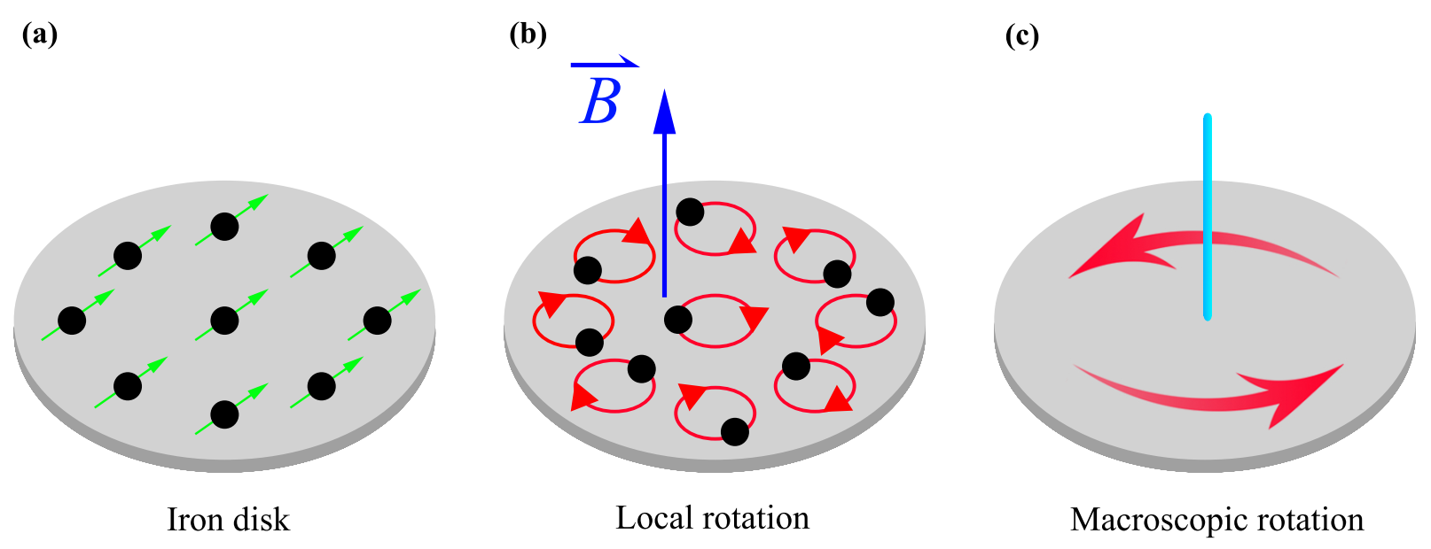
Figure 1: Schematic diagram of SRC mechanism in an iron disk. (a) Initial ferromagnetic configuration. (b) After the application of an external magnetic field $\bm{B}$ in the $z$-direction, the change in spin angular momentum causes atomic motion, resulting in local rotation of the disk. (c) The microscopic rotational “message” is transmitted throughout the disk at the speed of sound, leading to the macroscopic EdH rotation, as discussed in Refs. [1, 2].

Magnetization-rotation coupling is an intriguing and long-lasting topic. Owen W. Richardson (1908) first proposed that the moment of momentum is proportional to the magnetization using Ampère’s molecular currents [3]. Soon after, a gyromagnetic effect in macroscopic bodies was observed in the EdH experiment [4] (change of magnetization induces mechanical rotation) and the inverse Barnett experiment [5] (mechanical rotation triggers magnetization). In that period, molecular orbital theory was used to explain the EdH effect—the external magnetic field affected the angular momentum generated by electron orbital motion, leading the iron cylinder in the experiment to produce a mechanical angular momentum [6]. However, the discovery of electron spin reveals that the gyromagnetic ratio (ratio of magnetic moment to angular momentum) measured experimentally is close to the gyromagnetic ratio of the spin, $e/m$, which is twice the value predicted by considering only electron orbital motion [7]. It is now widely recognized that spin is an essential origin of magnetism and that the spin-lattice coupling is indispensable for the gyromagnetic effect. For transition metals like iron, the electronic orbital angular momentum can be readily frozen by the surrounding crystal field, resulting in a dominant contribution of spin to the magnetic moment. In a contemporary interpretation of the EdH effect, the conservation of total angular momentum is a basic principle, i.e., any change in the spin angular momentum requires a corresponding compensation of the mechanical angular momentum.

At the microscopic level, the mechanism via which angular momentum is transferred from electrons to the entire body remains elusive, as it is insufficient to explain the EdH effect by the conservation of angular momentum alone. Researchers firstly pay attention to those EdH effects occurring at the molecular scale due to finite degrees of freedom. For instance, the EdH effect is studied for a system of two dysprosium atoms trapped in a spherically symmetric harmonic potential [8]. A noncollinear tight-binding model capable of simulating the EdH effect of an $\mathrm{O_{2}}$ dimer has been proposed [9]. With the development of molecular-spintronics [10, 11, 12, 13], the problem of single spin embedded within a macroscopic object has gained attention [14, 15, 16]. The concept of phonon spin is used to explicate the spin-phonon coupling involved [17]. The orbital part and the spin part of phonon angular momentum (now considered pseudo-angular momentum [18]) are clearly divided in Refs. [19] and [20], where their exchange with (real) spin angular momentum are also discussed. Experiments have progressed to realize the coupling of single-molecule magnets with nanomechanical resonators [21]. Nevertheless, the multiatomic EdH effect, which involves numerous degrees of freedom, is inadequately comprehended despite the use of micromagnetic simulations [22, 23, 24, 25]. The mechanical dynamics of a magnetic cantilever resulting from changes in magnetization has also been described [26, 27, 28], but only one-sidedly considering the effect of spin evolution on lattice mechanics. Therefore, it is desired to develop a method that treats spin and lattice as equally important and converts the microscopic mechanism of the EdH effect into a macroscopic gyroscopic effect.

In this paper, we utilize Lagrangian formalism in classical field theory to derive spin-lattice dynamical equations in an elastic ferromagnet, where spins are coupled by exchange interactions. We assume that the magnetism of iron originates from the electronic spin, $\bm{M}=\gamma\hbar\bm{S}$, where $\bm{M}$ is magnetic moment, $\hbar$ is the Planck’s constant, $\gamma=ge/2m_{e}$ is the gyromagnetic ratio, and $g$ factor is 2 for spin $\bm{S}$. By means of the spin-rotation Hamiltonian arising from the conservation of spin angular momentum and mechanical angular momentum, a theoretical framework for the spin-lattice coupling is constructed—the change of magnetization results in a force on the atom, whereas the evolution of atomic displacement produces a torque acting on the spin. Then, we numerically solve the SRC dynamical equations in an iron disk to reveal the transfers of angular momentum and energy, thereby validating the EdH effect. The characteristics exhibited during the coupling process, such as the timescale of transfer and the dependence of the rotation frequency of the system on magnetic field and material parameters, can enhance the comprehension for laser-induced ultrafast demagnetization in solids [29, 30, 31, 32]. Exploring the mutual transfer of mechanical angular momentum and spin angular momentum can aid in creating new mechanical techniques for manipulating electron spins, or alternatively, using spins to manipulate mechanical motion.

This work is organized as follows. The spin-rotation Hamiltonian and dynamics equations merging spin and lattice are shown in Section II. The numerical method of applying the coupling equations to a disk model is introduced in Section III. And in Section IV, the pictures of angular momentum and energy transfers with and without damping are presented. The effects of the magnetic field on the rotation frequency and spin-relaxation time of the system are also discussed. And the Barnett effect is briefly described through the corresponding spin dynamics equation. In Section V, we draw conclusions and propose some further promising research ideas on spin-lattice coupling.

II spin-rotation Hamiltonian and coupling dynamical equations

For a stationary elastic magnet, when it is stimulated by an external field like a magnetic field or heat bath, the spins within the magnet will undergo a flipping process. As the system relaxes back to equilibrium, the magnet generates mechanical rotation locally, and subsequently overall, to preserve the total angular momentum of the system [1]. This interaction between spins and lattice is called SRC, and a visual representation of it is depicted in Figure 1. Recently, a study using ultrafast electron diffraction to probe lattice dynamics after femtosecond laser excitation has captured the transfer of angular momentum from spins to circularly polarized phonons, which can be considered as direct evidence in support of SRC [2].

Clearly, a magnetic moment $\bm{{M}}$ corresponds to an internal angular momentum, $\gamma^{-1}\bm{{M}}$. In the absence of external moments, the mechanical angular momentum $\bm{{L}}$ and the internal angular momentum $\gamma^{-1}\bm{{M}}$ should satisfy the conservation of total angular momentum,

$$\bm{{L}}+\gamma^{-1}\bm{{M}}=\mathrm{{constant}}.$$ (1)

As $\bm{{M}}$ evolves with time, a mechanical torque appears [16],

$$\bm{{T}}=-\gamma^{-1}\dot{\bm{{M}}}.$$ (2)

By denoting $\bm{\phi}_{i}$ as the local lattice rotation at site $i$ and considering the relationship $\bm{M}=\gamma\hbar\bm{S}$, the spin-rotation Hamiltonian can be expressed as

$$H_{\mathrm{s-r}}=-\sum_{i}\bm{{T}}\cdot\bm{\phi}_{i}=\sum_{i}\hbar\dot{\bm{S}}_{i}\cdot\bm{\phi}_{i}.$$ (3)

Eq. (3) incorporates the rate of change of the spins and the rotational motion of the lattice, enabling the transfer of angular momentum and energy between the spins and the lattice. A coupling term with similar form to $H_{\mathrm{s-r}}$ can be deduced by exploiting the rotation invariance of the magnetic anisotropy [27]. The orientation of a spin affects its energy, indicating that the magnetic anisotropy arises as a consequence of spin-lattice coupling. The specific form of magnetic anisotropy is generally determined by the symmetry of the system [33, 34]. Here, we additionally present two common coupling mechanisms that can also be studied using the following procedure. Firstly, the coupling between spins and lattice can be described in terms of Zeeman energy, where the local rotation of material is equated to the magnetic field, acting on the spins [16, 35]. Secondly, spins and lattice are coupled in the form of uniaxial magnetic anisotropy, which emerges from the perspective that lattice deformation can uniaxially pull the crystal field [19, 36, 37].

Next, we introduce other interactions in the system. The spin $\bm{S}_{i}$ at $i$th site can be decomposed into two mutually perpendicular components,

$$\bm{S}_{i}=\bm{\mu}_{i}+\bm{n}_{i}\sqrt{S^{2}-\mu_{i}^{2}},$$ (4)

where $\bm{\mu}_{i}\cdot\bm{n}_{i}=0$, but the orientations of themselves are arbitrary. $S$ is the size of the spin. In terms of $\bm{\mu}_{i}$, $\bm{n}_{i}$ and $\bm{u}_{i}$ (the displacement of the $i$th atom), the kinetic energy of the system can be written as [38]

$$T=\frac{\hbar}{2S}\sum_{i=1}(\dot{\bm{\mu}}_{i}\times\bm{n}_{i})\cdot\bm{\mu}_{i}+\sum_{i=1}\frac{1}{2}m_{i}\dot{\bm{u}}^{2}_{i},$$ (5)

with $m_{i}$ the mass of the $i$th atom. The first term represents the spin kinetic energy and the second term represents the lattice kinetic energy.

The total potential energy contains the Heisenberg exchange interaction $H_{\mathrm{ex}}$, the external Zeeman energy $H_{Z}$ and the crystal elastic energy $H_{\mathrm{e}}$ [39],

$$H_{\mathrm{ex}} =-\frac{1}{2}\sum_{ij}I_{ij}\bm{S}_{i}\cdot\bm{S}_{j},$$ (6)

$$H_{Z} =\sum_{i}g\mu_{B}\bm{B}\cdot\bm{S}_{i},$$ (7)

$$H_{\mathrm{e}} =\frac{1}{2}\int d^{3}r~{}\sigma_{\alpha\beta}u_{\alpha\beta}.$$ (8)

Here $I_{ij}$ is the ferromagnetic exchange coupling between $i$th and $j$th sites, $\mu_{B}$ is the Bohr magneton, $\bm{B}$ is the external magnetic field, and $\sigma_{\alpha\beta}$, $u_{\alpha\beta}$ are respectively the $(\alpha,\beta)$ components of the stress tensor and strain tensor with directional indexes $\alpha$, $\beta$.

Considering the large difference between the system size and interatomic distance, as well as the relatively low-energy associated with the transfer in comparison to the overall energy of the system, we treat the medium as continuous and employ the displacement field $\bm{u}(\bm{r},t)$ and the spin field $\bm{S}(\bm{r},t)$ at position $\bm{r}$ and time $t$ to describe the degrees of freedom of lattice and spin, respectively. For linearly elastic materials, $\sigma_{\alpha\beta}$ and $u_{\alpha\beta}$ conform to Hooke’s law, $u_{\alpha\beta}=(\nabla_{\alpha}u_{\beta}+\nabla_{\beta}u_{\alpha})/2$, $\sigma_{\alpha\beta}=C_{\alpha\beta\gamma\delta}u_{\gamma\delta}$, where $C_{\alpha\beta\gamma\delta}=\mathcal{R}_{~{}\alpha}^{\mu}\mathcal{R}_{~{}\beta}^{\nu}\mathcal{R}_{~{}\gamma}^{\sigma}\mathcal{R}_{~{}\delta}^{\rho}C_{\mu\nu\sigma\rho}$ with the coefficient tensor $C$, rotation transformation matrix $\mathcal{R}$, and directional indexes $\gamma$, $\delta$.

We express the local rotation $\bm{\phi}$ in terms of $\bm{u}(\bm{r},t)$ [40],

$$\bm{\phi}(\bm{r},t)=\frac{1}{2}\nabla\times\bm{u}(\bm{r},t),$$ (9)

and define the spin density $\bm{S}^{\prime}=\bm{S}/V$, where $V$ is the volume of the primitive cell and $\bm{S}$ is the total spin within $V$. With these variables, the spin-rotation Hamiltonian in Eq. (3) becomes

$$H_{\mathrm{s-r}}=\frac{1}{2}\int d^{3}r~{}\hbar\dot{\bm{S}}^{\prime}\cdot(\nabla\times\bm{u}).$$ (10)

For the nearest neighbor Heisenberg term, we approximate it by the Taylor expansion, whereby $\bm{S}_{j}=\bm{S}_{i+\delta_{j}}=\bm{S}_{i}+(\bm{\delta}_{j}\cdot\nabla)\bm{S}_{i}+\frac{1}{2}(\bm{\delta}_{j}\cdot\nabla)^{2}\bm{S}_{i}$ and $\bm{\delta}_{j}=\bm{S}_{j}-\bm{S}_{i}$. Since the Taylor expansion form is restricted by the high rotational symmetry, other lattice choices introduce nothing but the coefficient difference, which can be absorbed further into parameter selection, thus we take the square lattice as an example. In order to correctly obtain the spin dynamics equation, technically, we fix the direction of $\bm{n}$, $\partial\bm{n}/{\partial t}=0$. The disk material is considered isotropic with $I_{ij}=I$ for simplicity. We replace $\bm{S}_{i}$ and $\bm{u}_{i}$ with $\bm{S}(\bm{r},t)$ and $\bm{u}(\bm{r},t)$, respectively, and introduce the definitions $\bm{\mu}^{\prime}=\bm{\mu}/V$, $S^{\prime}=S/V$ and $I^{\prime}=I\times V$. Under Eqs. (5)-(8), (10), the Lagrangian density of the system reads,

$$\mathcal{L}= \frac{\hbar}{2S^{\prime}}(\dot{\bm{S}^{\prime}}\times\bm{n})\cdot\bm{S}^{\prime}+\frac{1}{2}\rho\dot{\bm{u}}^{2}+\frac{I^{\prime}}{2}\bm{S}^{\prime}\cdot[\bm{S}^{\prime}+a^{2}\nabla^{2}\bm{S}^{\prime}]$$

$$-g\mu_{B}\bm{B}\cdot\bm{S}^{\prime}-\frac{1}{2}C_{\alpha\beta\gamma\rho}u_{\gamma\rho}u_{\alpha\beta}-\frac{1}{2}\hbar\dot{\bm{S}}^{\prime}\cdot(\nabla\times\bm{u}),$$ (11)

where $\rho$ is the mass density of the material and $a$ is the lattice constant. According to the Euler-Lagrange equations in classical field theory,

$$\frac{d}{dt}\frac{\partial\mathcal{L}}{\partial\dot{u}_{\alpha}}+\nabla\cdot\frac{\partial\mathcal{L}}{\partial(\nabla u_{\alpha})}=\frac{\partial\mathcal{L}}{\partial u_{\alpha}},$$ (12a)

$$\frac{d}{dt}\frac{\partial\mathcal{L}}{\partial\dot{S}_{\alpha}^{\prime}}=\frac{\partial\mathcal{L}}{\partial S_{\alpha}^{\prime}},$$ (12b)

with $\alpha=x$, $y$, and $z$, the spin-lattice dynamic equations can be derived,

$$\rho\frac{\partial^{2}\bm{u}}{\partial t^{2}}-\nabla\cdot\bm{\sigma}+\frac{1}{2}\nabla\times\hbar\dot{\bm{S}^{\prime}}=0,$$ (13)

$$\hbar\dot{\bm{S}}=\bm{S}\times\left[Ia^{2}\nabla^{2}\bm{S}-g\mu_{B}\bm{B}+\frac{\hbar}{2}(\nabla\times\dot{\bm{u}})\right].$$ (14)

Eqs. (13) and (14) tell us that the time evolution of the spin field acts as a driving force $\bm{f}^{(R)}=-(\nabla\times\hbar\dot{\bm{S}}^{\prime})/2$ on the displacement field, and in turn, the evolution of the displacement field produces a torque $\hbar(\nabla\times\dot{\bm{u}})/2$ acting on the spin. Note that the entire rotation contributes to $\nabla\times\dot{\bm{u}}$.

Let us now turn to angular momentum. By previous discussion (see Eq. (1)), the total angular momentum (spin and mechanical) can be represented as

$$\bm{J}=\int d^{3}r~{}[\hbar\bm{S}^{\prime}+\rho(\bm{r}\times\dot{\bm{u}})].$$ (15)

For the time derivative of the $\alpha$-component of $\bm{J}$,

$$\dot{J}_{\alpha}=\int d^{3}r~{}\hbar\dot{S}_{\alpha}^{\prime}+\int d^{3}r~{}\epsilon_{\alpha\beta\gamma}r_{\beta}\rho\ddot{u}_{\gamma},$$ (16)

the following expression can be obtained by using Eq. (13) and performing a partial integration taking into account the symmetry of $\sigma_{\alpha\beta}$,

$$\dot{J}_{\alpha}=\int dA_{\delta}~{}\epsilon_{\alpha\beta\gamma}r_{\beta}\sigma_{\gamma\delta}+\frac{1}{2}\int dA_{\eta}~{}r_{\eta}\hbar\dot{S}_{\alpha}^{\prime}-\frac{1}{2}\int dA_{\alpha}~{}r_{\beta}\hbar\dot{S}_{\beta}^{\prime}.$$ (17)

Here $dA_{\delta}$, $dA_{m}$, and $dA_{\alpha}$ refer to the boundary surfaces in the $\delta,m,\alpha=x,y,z$ directions.

III numerical solution for a disk model

A quasi-two-dimensional disk model depicted in Figure 1 is adopted to solve Eqs. (13) and (14). In general, the coefficient tensor $C_{\alpha\beta\gamma\delta}$ is a $9\times 9$ matrix. However, for an isotropic object with symmetric stress and strain tensors, $C_{\alpha\beta\gamma\delta}$ can be described only by two independent elastic moduli $\lambda$ and $\mu$ [41], $C_{\alpha\beta\gamma\delta}=\lambda\delta_{\alpha\beta}\delta_{\gamma\delta}+\mu(\delta_{\alpha\gamma}\delta_{\beta\delta}+\delta_{\alpha\delta}\delta_{\beta\gamma})$. Hooke’s law relates it to the stress tensor, $\sigma_{\alpha\beta}=E/(1+\nu)[u_{\alpha\beta}+(\nu/1-2\nu)u_{\gamma\gamma}\delta_{\alpha\beta}]$, where $E$ is Young’s modulus given by $E={\mu(3\lambda+2\mu)}/({\lambda+\mu})$, and $\nu$ is Poisson’s coefficient, defined as $\nu={\lambda}/{2(\lambda+\mu)}$. Polar coordinates are more convenient for the complanate and axisymmetric disk system (a detailed derivation of coordinate transforation is provided in Appendix A). Assuming plain strain and solely considering $\theta$-invariant solutions, we can establish that $u_{az}=u_{za}=0$, $\nabla_{z}S_{a}=0$, $\nabla_{\theta}u_{a}=0$ and $\nabla_{\theta}S_{a}=0$, where $a\in\{r,\theta,z\}$.

To clearly demonstrate the influence of material properties on the evolution of the system, we substitute all variables with dimensionless counterparts, which are defined as follows,

$$\overline{u}_{\theta}=\frac{u_{\theta}}{R},\overline{r}=\frac{r}{R},\overline{\bm{S}}=\frac{\bm{S}}{S},\overline{t}=tm,m\equiv\sqrt{\frac{E}{2(1+\nu)\rho R^{2}}},$$ (18)

where $R$ is the radius of the disk. The dynamical equations for $\overline{u}_{\theta}$ (the displacement variable associated with the rotation of the disk) and $\overline{\bm{S}}$ in polar coordinates can be derived from Eqs. (13) and (14) (for further calculation details, please refer to Appendix A),

$$\frac{\partial^{2}\overline{u}_{\theta}}{\partial\overline{r}^{2}}+\frac{1}{\overline{r}}\frac{\partial\overline{u}_{\theta}}{\partial\overline{r}}-\frac{1}{\overline{r}^{2}}\overline{u}_{\theta}=\frac{\partial^{2}\overline{u}_{\theta}}{\partial\overline{t}^{2}}+K\overline{f}_{\theta},$$ (19)

$$\frac{\partial\overline{\bm{S}}}{\partial\overline{t}} =\overline{\bm{S}}\times[\alpha_{1}(\frac{\partial^{2}}{\partial\overline{r}^{2}}+\frac{1}{r}\frac{\partial}{\partial\overline{r}})\overline{\bm{S}}+\frac{1}{2}\left(\frac{\partial^{2}}{\partial\overline{r}\partial\overline{t}}+\frac{1}{\overline{r}}\frac{\partial}{\partial\overline{t}}\right)\overline{{u}}_{\theta}\bm{e}_{z}$$

$$\quad-\beta_{1}\bm{e}_{z}].$$ (20)

The coupling coefficient $K=\hbar SS_{0}\sqrt{(1+\nu)/2E\rho R^{2}}$ (with $S_{0}$ representing the constant spin density [27]), $\alpha_{1}=Ia^{2}S/\hbar R^{2}m$, $\beta_{1}=g\mu_{B}B/\hbar m$, and $\overline{f}_{\theta}=\partial^{2}\overline{S}_{z}/\partial\overline{t}\partial\overline{r}$. In the present paradigm, the strength of the SRC exhibits correlations with elastic coefficients ($E$ and $\nu$), density ($\rho$), and exchange interaction ($I$).

Also, based on Eq. (17), the time derivative of angular momentum in polar coordinates is given,

$$\dot{J}_{r} =0,$$ (21a)

$$\dot{J}_{\theta} =\frac{1}{2}\int dA_{r}~{}r\hbar\dot{S}_{\theta},$$ (21b)

$$\dot{J}_{z} =\int dA_{r}~{}r\sigma_{r\theta}+\frac{1}{2}\int dA_{r}~{}r\hbar\dot{S}_{z}.$$ (21c)

In this case, the angular momentum in the $r$-direction, $J_{r}$, is automatically conserved.

Damping is ubiquitous in most situations. To account for this effect, we introduce the first-order time derivative of $u_{\theta}$ into Eq. (19) and integrate the Gilbert damping [42] into Eq. (III), leading to a coupled system with damping,

$$\frac{\partial^{2}\overline{u}_{\theta}}{\partial\overline{r}^{2}}+\frac{1}{\overline{r}}\frac{\partial\overline{u}_{\theta}}{\partial\overline{r}}-\frac{1}{\overline{r}^{2}}\overline{u}_{\theta}=\frac{\partial^{2}\overline{u}_{\theta}}{\partial\overline{t}^{2}}+K\overline{f}_{\theta}+\eta\frac{\partial\overline{u}_{\theta}}{\partial\overline{t}},$$ (22)

$$\dot{\overline{\bm{S}}}=\overline{\bm{S}}\times\overline{\bm{\Gamma}}+\zeta(\dot{\overline{\bm{S}}}\times\overline{\bm{S}}),$$ (23)

where

$$\overline{\bm{\Gamma}} =\alpha_{1}(\frac{\partial^{2}}{\partial\overline{r}^{2}}+\frac{1}{r}\frac{\partial}{\partial\overline{r}})\overline{\bm{S}}+\frac{1}{2}\left(\frac{\partial^{2}}{\partial\overline{r}\partial\overline{t}}+\frac{1}{\overline{r}}\frac{\partial}{\partial\overline{t}}\right)\overline{{u}}_{\theta}\bm{e}_{z}$$

$$\quad-\beta_{1}\bm{e}_{z},$$ (24)

and $\eta$ (¿0), $\zeta$ are dimensionless damping factors.

We employ a finite difference method to solve the coupled partial differential Eqs. (22) and (23). Under specific boundary and initial conditions (which will be provided later), once the time evolutions of the displacement field and spin field are clear, the mechanical angular momentum, the spin angular momentum, and the various energy terms can be subsequently calculated.

\begin{overpic}[scale={0.15}]{angular_nodamping.png} \put(-2.0,68.0){\large{(a)}} \end{overpic}

\begin{overpic}[scale={0.15}]{angular_damping.png} \put(-2.0,68.0){\large{(b)}} \end{overpic}

Figure 2: Evolution of the time derivative of angular momentum in the $z$-direction. $\dot{J}_{S}$ corresponds to the spin angular momentum, $\dot{J}_{L}$ to the mechanical angular momentum, and $\dot{J}_{\mathrm{d}}$ to the angular momentum loss. (a) Undamped case, $\dot{J}_{\mathrm{totoal}}=\dot{J}_{S}+\dot{J}_{L}$. (b) Damped case, $\dot{J}_{\mathrm{total}}=\dot{J}_{S}+\dot{J}_{L}+\dot{J}_{\mathrm{d}}$. Damping factors $\eta=0.5$ and $\zeta=0.5$ are used. The large damping coefficients are chosen to display the final state of the system.

IV results and analysis

IV.1 Transfer of angular momentum

We focus on the angular momentum in the $z$-direction, as it is relevant to the rotation of the disk. Following from the $z$-component of Eq. (16), the time derivative of the spin angular momentum is

$$\dot{J}_{S}=\int d^{3}r~{}\hbar\dot{S}_{z},$$ (25)

and the time derivative of the mechanical angular momentum is

$$\dot{J}_{L}=\int d^{3}r~{}\rho r\ddot{u}_{\theta}.$$ (26)

When solving Eqs. (22) and (23), we specify the boundary conditions as

$$\left\{\begin{aligned} &\sigma_{r\theta}=0,~{}\sigma_{rr}=0\qquad\mathrm{when~{}}r\to 0\\ &\sigma_{r\theta}=0,~{}\sigma_{rr}=0\qquad\mathrm{at~{}}r=R\end{aligned}\right.\qquad\mathrm{for~{}}u_{\theta},$$ (27)

and

$$\left\{\begin{aligned} &\dot{J}_{\theta}=0,~{}\dot{J}_{z}=0\qquad\mathrm{when~{}}r\to 0\\ &\dot{J}_{\theta}=0,~{}\dot{J}_{z}=0\qquad\mathrm{at~{}}r=R\end{aligned}\right.\qquad\mathrm{for~{}}\bm{S}.$$ (28)

The selection of $r\to 0$ as a boundary instead of $r=0$ stems from the requirement to ensure the validity of the formula $1/r$. The explicit formulations of $\sigma_{r\theta}$ and $\sigma_{rr}$ can be found in Appendix A. The first two conditions on $u_{\theta}$ correspond to the absence of force at the two boundaries, while the last two conditions on $\bm{S}$ guarantee the total angular momentum of the system cannot flow out from the boundaries.

Since the iron disk is ferromagnetic, the following initial conditions are taken—at the beginning, all the spins on the disk are uniformly aligned, and both atomic displacement and velocity are zero (i.e., the disk is stationary). It should be emphasized that our approach extends beyond the initial circumstances, and as will be seen later, we deliberately choose other initial conditions to effectively illustrate the energy transfer process.

IV.1.1 Undamped and damped cases

The selected magnetic material for this study, Fe, possesses an exchange parameter of $I=4.29\times 10^{-21}\mathrm{~{}J}$, a lattice constant of $a=2.87\times 10^{-10}\mathrm{~{}m}$, a mass density of $\rho=7.9\times 10^{3}\mathrm{~{}kg/m^{3}}$, Young’s modulus of $E=1.85\times 10^{11}\mathrm{~{}Pa}$, and Poisson’s coefficient of $\nu=0.32$, as reported by [22]. The disk radius is set to $R=10^{-7}~{}\mathrm{m}$. Unless otherwise noted, these parameters are consistently used in the calculations that follow.

To provide a comprehensive analysis, both damped and undamped results are presented in Figure 2. The variable $\dot{J}_{d}$, as shown in Figure 2, represents the rate of change of angular momentum loss attributed to the displacement damping ($\eta$). According to Equation (22), the damping term introduces a resistive force acting on the atom, described by $F_{\mathrm{d}}^{\theta}=-\eta~{}{\partial u_{\theta}}/{\partial t}$. This leads to the emergence of a torque in the $z$-direction, which can be equivalently expressed as the time derivative of the angular momentum,

$$\dot{J}_{\mathrm{d}}=-\eta\int d^{3}r~{}r\frac{\partial u_{\theta}}{\partial t}.$$ (29)

Figure 2 illustrates that at $t=0$, the rates of change of spin angular momentum and mechanical angular momentum are zero due to the initial conditions of the system. However, at the next moment of the numerical calculation, the magnetic field $B=1\mathrm{~{}T}$ is applied in the disk, resulting in non-zero rates of change of angular momentum (see Eqs. (22), (23), (25), and (26)). Especially in the presence of damping, both the driving force, denoted as $\overline{f}_{\theta}$, and the first-order time derivative of the displacement field, represented by $\dot{u}_{\theta}$, are no longer zero after the introduction of the magnetic field, causing an abrupt increase in the second-order time derivative of the displacement field $\ddot{u}_{\theta}$, i.e., a sharp jumping in the rate of change of the mechanical angular momentum in Figure 2. This phenomenon indicates that the external magnetic field acts as the driving source for the EdH effect. If the driving source is the rotation of the magnet (no external magnetic field in this case), the evolution of the displacement field will result in spin-flips, similar to the Barnett effect. Notably, between $t=0.25~{}\mathrm{ns}$ and $t=0.35~{}\mathrm{ns}$, there is a strange peak, which can be suppressed by a stronger magnetic field, suggesting its intrinsic cause is the competition between the external magnetic field and the intrinsic elastic dynamics. Overall, in the absence of damping, $\dot{J}_{L}$ and $\dot{J}_{S}$ exhibit a high-frequency periodic behavior in Figure 2. The correlation between the oscillation frequency and the strength of the external magnetic field as well as material properties will be discussed in subsequent sections.

Another crucial factor closely related to spin-mechanical applications is the timescale of angular momentum transfer. It has been discovered that after impinging magnetized material with an ultrafast laser, electronic spins transfer their angular momentum to atoms within the lattice in just a few hundred femtoseconds, leading to the creation of circularly polarized phonons which then propagate the angular momentum throughout the entire material at the speed of sound, ultimately contributing to the macroscopic EdH rotation [2]. Drawing on this research, we roughly estimate the time it takes for the angular momentum to transfer from local rotation (circularly polarized phonons) to macroscopic rotation, $t\approx R/v=0.02~{}\mathrm{ns}$, with the speed of sound $v\propto\sqrt{E/\rho}$. This timescale is reflected in our theoretical results. In Figure 2, when $t=0.02~{}\mathrm{ns}$, the rate of change of the angular momentum at this point is large enough to indicate the occurrence of macroscopic rotation. Considering that the coefficient factor of $v$ is undetermined, we estimate the timescale for the transfer of spin angular momentum to the whole lattice to be on the order of 0.01 ns. Nevertheless, accurately evaluating the femtosecond timescale for the transfer of angular momentum from spin to local rotation is currently unfeasible due to the inability to precisely identify the exact moment when local rotation emerges.

Throughout the coupling process, the rate of change of the spin angular momentum ($\dot{J}_{S}$) and the rate of change of the lattice angular momentum ($\dot{J}_{L}$, or the sum of $\dot{J}_{L}$ and $\dot{J}_{\mathrm{d}}$ in the damped case) evolve inversely, with their sum remaining at zero. This observation demonstrates the interconversion of the spin angular momentum and the lattice angular momentum, while the total angular momentum is conserved. As our approach is not constrained by initial conditions, it allows exploring the spin-lattice coupling processes where the system start from a nonequilibrium or nonferromagnetic configuration. First-principle calculations can assist in calculating the initial spin configurations of diverse materials. Besides, the dynamic behavior of magnetic systems under external perturbations, including magnetic field and stress, can also be investigated. By incorporating the effects of these perturbations into the coupling equations, one can analyze the response and sensitivity of the system to different stimuli and predict their influences on the dynamical evolution from lattice to spin or from spin to lattice.

It is worth mentioning that there is another type of angular momentum involved here, namely pseudoangular momentum [18] or angular momentum in field theory [19]. Unlike the traditional angular momentum under Newtonian mechanics, the conservation of pseudoangular momentum arises from the rotational invariance of the Lagrangian with respect to the rotation of the spin and displacement fields,

$$\bm{u}(\bm{r})\rightarrow\mathcal{R}\bm{u}(\mathcal{R}^{-1}\bm{r}),\quad\bm{S}(\bm{r})\rightarrow\mathcal{R}\bm{S}(\mathcal{R}^{-1}\bm{r}).$$ (30)

Here, the rotation $\mathcal{R}$ is restricted to rotations around the $z$-axis because of the magnetic field. By substituting Eq. (30) into Eq. (II), a simple analysis shows that the Lagrangian density is invariant and the relevant conserved quantity derived from Noether’s theorem [43] is the pseudoangular momentum.

\begin{overpic}[scale={0.15}]{magnetic_frequency.png} \put(0.0,73.0){\large{(a)}} \end{overpic}

\begin{overpic}[scale={0.15}]{M_z.png} \put(0.0,75.0){\large{(b)}} \end{overpic}

\begin{overpic}[scale={0.15}]{relaxation_time.png} \put(0.0,75.0){\large{(c)}} \end{overpic}

Figure 3: Influence of the magnetic field on angular momentum transfer. (a) The oscillation frequency of angular momentum versus the magnetic field $B$. In the linear fitting, $k_{1}=4.493$ and $b_{1}=0.1367$. (b) Magnetization evolution under different magnetic fields. Damping factors $\eta=0.5$ and $\zeta=0.5$. The inset shows the case without damping, but with magnetic field $B=1~{}\mathrm{T}$. (c) Spin-lattice relaxation time versus $B$. The solid line (shown in red) represents an inverse proportional fitting with $a=0.19$.

IV.1.2 Effect of magnetic field

The previous description is based on applying a constant magnetic field to the disk, but it is important to note that an oscillating magnetic field can also be employed without significantly altering the main conclusions. To maintain focus, we will study the effect of the constant magnetic field on the evolution of the system. We define the oscillation frequency of angular momentum as the number of oscillations per second, and its relationship with the magnetic field is depicted in Figure 3. When there is no damping, the frequency is proportional to the magnitude of the magnetic field, $f\propto B$, where the proportionality constant is the slope of the linear fitting, $k_{1}$. Eq. (22) reveals two distinct types of displacement field evolution: intrinsic and forced. The former is governed by the purely elastic dynamics equation, and its oscillation frequency is determined by the material elasticity coefficients, while the latter is driven by the change of spin, with an oscillation frequency determined by the spin torque, $\dot{\bm{S}}=\bm{S}\times[Ia^{2}/\hbar\nabla^{2}\bm{S}+\gamma\bm{B}+(\nabla\times\dot{\bm{u}})/2]$. The linear relationship between the oscillation frequency and the external magnetic field suggests that above $B=0.1~{}\mathrm{T}$ (the magnetic field corresponding to the first data point in Figure. 3), the displacement field mainly follows forced oscillations. When the magnetic field equals $0.1~{}\mathrm{T}$, we compare the magnitude of spin torques generated by the Heisenberg term $Ia^{2}/\hbar\nabla^{2}\bm{S}$, the external magnetic field $\gamma\bm{B}$, and the displacement field $(\nabla\times\dot{\bm{u}})/2$. We find that the contribution from the displacement field is significantly smaller than that from the magnetic field. Moreover, although the Heisenberg interaction torque varyies with the spin itself, it is also lower than the magnetic field torque across most of the disk. Consequently, the external magnetic field dominates the evolution frequency of the spin and displacement fields, while the other two serve as modulating factors. This reminds us that in purely precessional dynamics of spin, the precession frequency is proportional to the effective field that induces spin precession [42], $\dot{\bm{S}}=\bm{S}\times\gamma\bm{H}_{\mathrm{eff}}$, $w=\lvert\gamma\bm{H}_{\mathrm{eff}}\rvert=2\pi f^{\prime}$, where $\bm{H}_{\mathrm{eff}}$ is the effective field, $w$ is the angular frequency, and $f^{\prime}$ is the frequency. After comparing $k_{1}$ and $\lvert\gamma/2\pi\rvert/10^{9}$, we discover that these two values are not equivalent, with $k_{1}$ being approximately one-sixth of the latter. If the spin torques solely contain the magnetic field term, the spins will precess around $\bm{B}$. This means that the spin angular momentum in the $z$-direction remains unchanged and is not transferred to the lattice system. In other words, despite the inferior effect on the oscillation frequency of the angular momentum, the Heisenberg term and the displacement field term play a crucial role in facilitating the transfer of angular momentum between the spins and lattice.

In the scenario of damping, our investigation aims at the dependence of the spin-lattice relaxation time on the magnetic field. For this purpose, we denote the $z$-component of magnetization intensity as $M_{z}$ and the saturation magnetization intensity as $M_{0}$. Figure 3 illustrates the dynamic behavior of $M_{z}$ under varying magnetic fields. When both the magnetic field and damping are present, all the spins end up pointing in the direction of the magnetic field, with the higher magnetic field leading to faster saturation of the magnetization. In contrast, without damping (as shown in the inset), the spins exhibit periodic oscillations and fail to align with the z-axis direction, despite being subjected to the magnetic field. Damping is essential in achieving a stable magnetization. The spin-lattice relaxation time is defined as the duration required for $M_{z}$ to reach $M_{0}$, which is considered achieved when the deviation is less than or equal to 0.02, i.e., $\Delta M^{z}/\Delta M\leqslant 0.02$, where $\Delta M^{z}=M_{0}-M_{z}$, $\Delta M=M_{0}-M_{z}^{t=0}$. As shown in Figure. 3, the relaxation time shows a significant decrease as the magnetic field increases from $1~{}\mathrm{T}$ to $2~{}\mathrm{T}$, and for large damping and magnetic fields of $B>1~{}\mathrm{T}$, it falls below 0.1 ns. Moreover, through data fitting, we observe an near-inverse correlation between the relaxation time and the magnetic field. This feature also appears in the Landau-Lifshitz-Gilbert (LLG) equation for the typical dissipation time $\tau_{LLG}$ [44], $\tau_{LLG}=1/w_{L}\zeta$, where $w_{L}$ is the precession frequency and $\zeta$ is the damping factor.

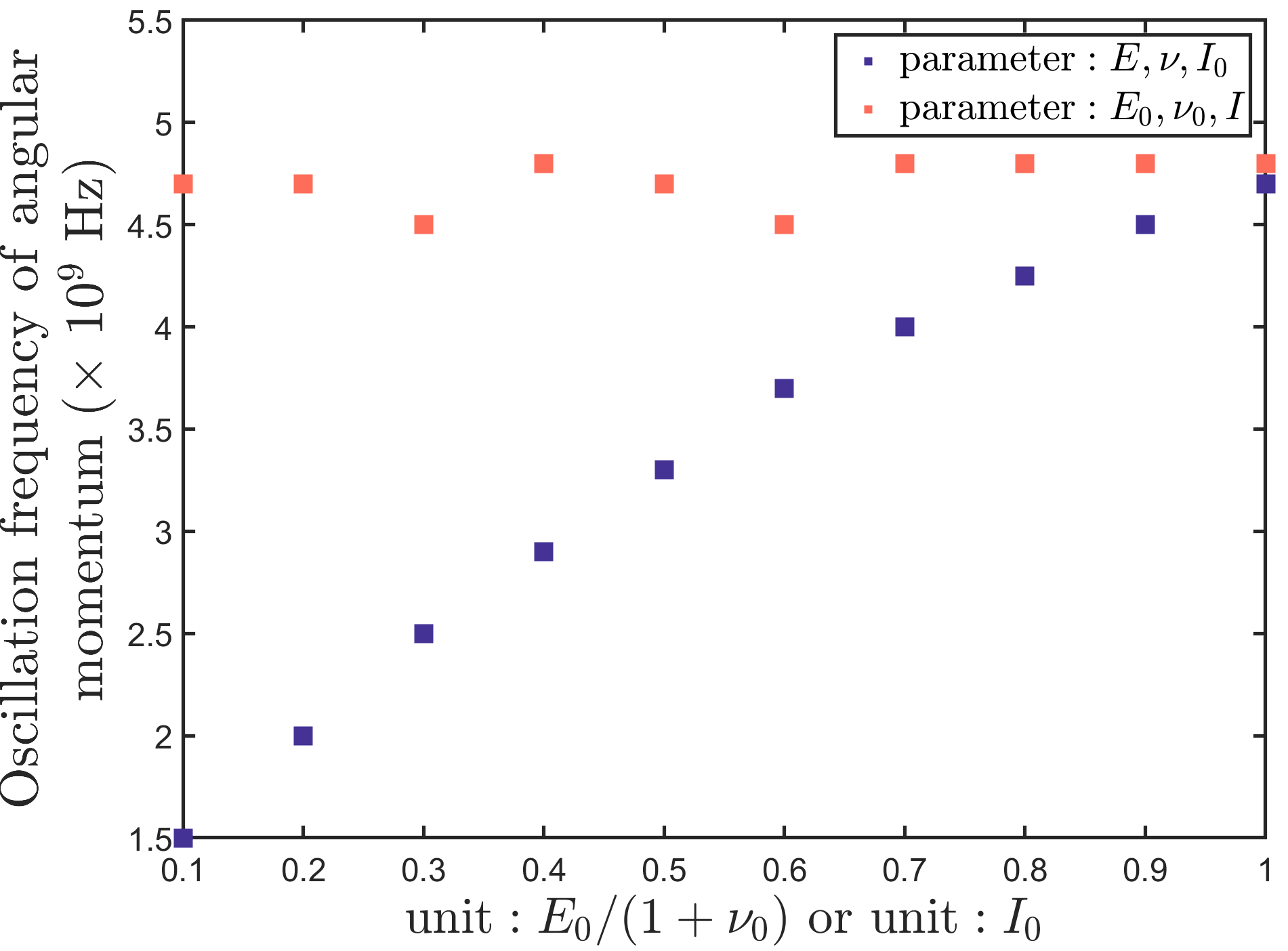
Figure 4: The oscillation frequency of angular momentum versus $E/(1+\nu)$ and $I$. Here, $E_{0}=1.85\times 10^{11}\mathrm{~{}Pa}$, $\nu_{0}=0.32$, $I_{0}=4.29\times 10^{-20}\mathrm{~{}J}$, and $B=0~{}\mathrm{T}$.

\begin{overpic}[scale={0.15}]{energy_nodamping.png} \put(-2.0,68.0){\large{(a)}} \end{overpic}

\begin{overpic}[scale={0.15}]{energy_damping.png} \put(-2.0,68.0){\large{(b)}} \end{overpic}

Figure 5: Evolution of each part of energy. $E_{\mathrm{ex}}$ represents the Heisenberg energy, $E_{u}$ includes the kinetic energy of the displacement field and elastic energy, $E_{z}$ is the Zeeman energy, $E_{\mathrm{d}}$ illustrates the effect of spin damping on the Zeeman term, and $E_{\mathrm{total}}$ is their sum. $\Delta$ denotes their change. (a) Undamped case with $B=2~{}\mathrm{T}$. (b) Damped case with $B=50~{}\mathrm{T}$, $\zeta=0.5$, and $\eta=0.5$. $B$ is set to $50~{}\mathrm{T}$ to amplify the variation of $E_{z}$.

IV.1.3 Effect of material parameters

Our calculations demonstrate that variations in material parameters, such as the exchange coefficient ($I$), Young’s modulus ($E$), and Poisson’s coefficient ($\nu$), can significantly impact the magnitude of the angular momentum while having minimal effect on its frequency when the system is exposed to a magnetic field. To explore the influence of material parameters on the system’s evolution, we exclude the magnetic field ($B=0$) and utilize the rotation of the disk as the driving force. The initial angular velocity chosen for this is the same as that used in the energy transfer case discussed below. In Figure. 4, the oscillation frequency of angular momentum ranges from $4.5\times 10^{9}$ Hz to $5\times 10^{9}$ Hz, with negligible dependence on $I$. This behavior is expected since $I$ does not directly affect the coupling coefficient $K$ for isotropic objects. However, for the elasticity coefficients $E$ and $\nu$, the frequency exhibits a positive correlation with the ratio of $E$ to $\nu$, although not in a linear manner like the magnetic field. The Young’s modulus of a material is a manifestation of its interatomic bonding energy and lattice structure. A larger $E$ to $\nu$ ratio indicates a harder material, which is more likely to move as a whole and less prone to local elastic deformation. This information is useful for selecting suitable elastic materials, whether they are softer or harder, as potential candidates for the spin-rotation devices.

IV.2 Transfer of energy

The EdH process also involves an energy exchange between the spin subsystem and lattice subsystem. Noether’s theorem states that the time translation invariance of the Lagrangian density (Eq. (II)) ensures the conservation of energy and the total energy is determined as

$$H =\int d^{3}r~{}\left[\frac{\partial\mathcal{L}}{\partial\dot{\Phi_{a}}}\Phi_{a}-\mathcal{L}\right]$$

$$=\int d^{3}r~{}\bigg{[}\frac{1}{2}\rho\dot{\bm{u}}^{2}-\frac{I^{\prime}}{2}\bm{S}^{\prime}\cdot(\bm{S}^{\prime}+a^{2}\nabla^{2}\bm{S}^{\prime})+g\mu_{B}\bm{B}\cdot\bm{S}^{\prime}$$

$$\quad+\frac{1}{2}C_{\alpha\beta\gamma\rho}u_{\gamma\rho}u_{\alpha\beta}\bigg{]},$$ (31)

where $\Phi_{a}=u_{a}$ and $S^{\prime}_{a}$. If the initial conditions mentioned in Section IV.1 persist, the lattice energy will start at a level lower than the spin energy due to the absence of lattice kinetic energy and the non-zero spin energy of the ferromagnetic ground state. To balance the consideration of spin and lattice, we adopt an initial state where the angular velocity disk is set at one $m~{}\mathrm{rad/s}$, with $m$ being the dimensionless factor of time in Eq. (18).

Figure 5 describes the energy conversion process with and without damping. In the undamped scenario, our focus lies on the changes in energy of each component, denoted as $\Delta E$, which are all much smaller than the components themselves. As depicted, the Zeeman term $\Delta E_{\mathrm{Z}}$ evolves opposite to both the exchange term $\Delta E_{\mathrm{ex}}$ and the lattice term $\Delta E_{\mathrm{u}}$. This represents the transfer of energy from the former to the latter two and a constant total energy. Similarly, a stronger magnetic field can help to smooth out the irregular curve observed between $t=0.3~{}\mathrm{ns}$ and $t=0.35~{}\mathrm{ns}$, again because of the competition between the external magnetic field and the intrinsic evolution. The Heisenberg energy $E_{\mathrm{ex}}$ is defined by Eq. (II), and it is directly proportional to $\bm{S}\cdot\nabla^{2}\bm{S}$. Consequently, we have $(\partial{E}_{\mathrm{ex}}/{\partial t})\propto\dot{\bm{S}}\cdot\nabla^{2}\bm{S}$, where the term $\nabla^{2}\dot{\bm{S}}$ is neglected as it is small compared to $\dot{\bm{S}}$. With this in mind, the energy dissipation arising from the magnetic field response to spin damping, $E_{\mathrm{d}}$, satisfies $(\partial E_{d}/\partial t)\propto-\dot{\bm{S}}_{\mathrm{damping}}\cdot g\mu_{B}\bm{B}$. Hence, the energy loss can be estimated as

$$E_{d}=-\int dt~{}g\mu_{B}\bm{B}\cdot[\frac{\zeta}{\hbar S}(\bm{S}\times\bm{\Gamma})\times\bm{S}].$$ (32)

The remaining energy losses caused by damping effects are outlined in Section B, and their cumulative value is denoted as $E_{\mathrm{damping}}$ in Figure 5. Under large damping conditions, the kinetic energy $E_{\mathrm{u}}$ rapidly drops to zero. It is clear that $E_{\mathrm{u}}$ is the primary contributor to energy loss, combined with the trend of the loss term $E_{\mathrm{damping}}$. The Zeeman energy is nearly offset by the damping term $E_{\mathrm{d}}$, as evidenced by their constant sum shown in the inset. The change in exchange energy $E_{\mathrm{ex}}$ is relatively insignificant compared to the other energy terms, thus its behavior is shown separately in the inset. Initially, $E_{\mathrm{ex}}$ rises sharply, then falls rapidly and becomes the first to stabilize. It should be noted that the damping factors used in the theoretical calculations are higher than the actual values, necessitating the use of realistic and appropriate damping factors to explore the specific transfer of each energy term in more intricate detail.

The impact of the magnetic field on the oscillating frequency of energy is illustrated in Figure 6. When the magnetic field is small, the oscillation frequency of energy decreases with increasing the magnetic field. However, once the magnetic field reaches approximately $1~{}\mathrm{T}$, the frequency starts to increase linearly with the magnetic field strength. In energy calculations, we consider a non-zero initial velocity for the disk, which drives the intrinsic evolution of the system. At relatively low magnetic fields, the initial rotation and the magnetic field jointly determine the frequency of the system, with the former contributing more. But, as the magnetic field continues to grow to about $1~{}\mathrm{T}$, the frequency approaches 0, indicating a competitive relationship between the two driving sources in determining the magnetic field. Increasing the field further, it will surpasse the influence of the initial conditions and become the dominant factor in determining the frequency. Furthermore, it is hypothesized that different magnetic materials and initial conditions would correspond to different critical magnetic fields. In addition, the slope of this linear correlation does not align with that of the zero initial velocity case depicted in Figure 3. In combination with the discussion in Section IV.1.2, it can be expected that the linear slope between the frequency and magnetic field is determined by the Heisenberg interaction, the spin-lattice coupling term, and the intrinsic evolution of the system. However, the precise connection between them is not addressed in this work.

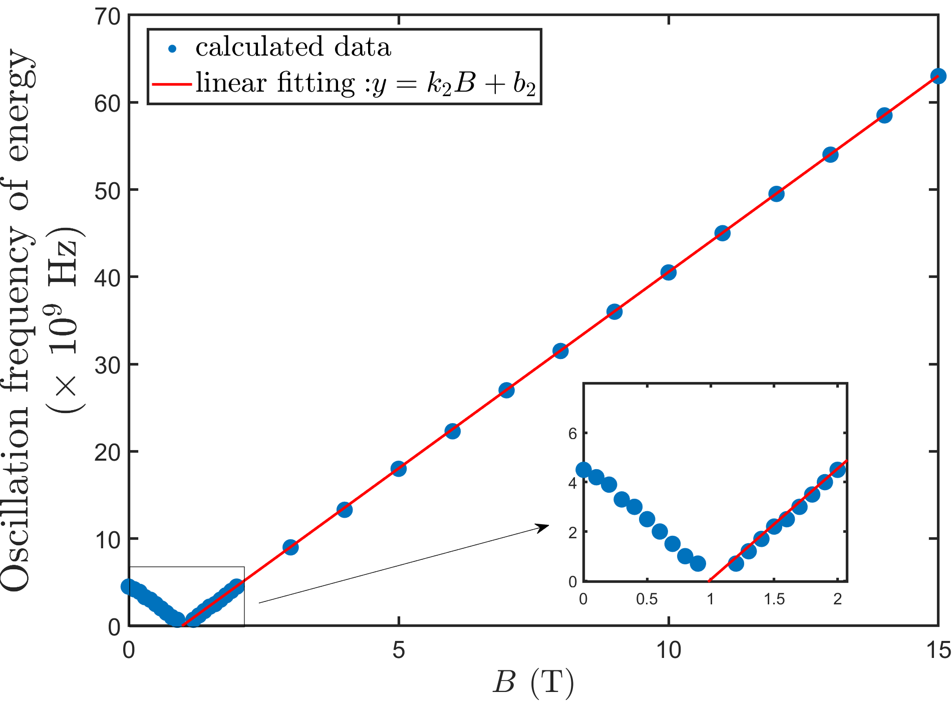
Figure 6: The oscillation frequency of energy versus the magnetic field $B$. In the linear fitting, $k_{2}=4.5$ and $b_{2}=-4.45$. The critical magnetic field (corresponding to the field at zero frequency) is about $1~{}\mathrm{T}$.

IV.3 Barnett effect

As the inverse effect of EdH, the Barnett effect is another manifestation of SRC. In this context, the displacement field follows an overall rotation with angular velocity $\bm{\Omega}$, $\bm{u}=r\bm{\Omega}t$, and Eq. (14), which governs the spin dynamics, degenerates to the following form,

$$\dot{\bm{S}}=\bm{S}\times(Ia^{2}/\hbar\nabla^{2}\bm{S}+\bm{\Omega}).$$ (33)

Eq. (33) reveals that the magnetization generated by rotating a ferromagnetic object at an angular velocity $\bm{\Omega}$ in the absence of a magnetic field is equivalent to that produced when the object is not rotating but subjected to a magnetic field $\bm{B}_{\mathrm{eff}}=\gamma\bm{\Omega}$. This phenomenon demonstrates the Barnett effect, and the effective field $\bm{B}_{\mathrm{eff}}$ is referred to as the Barnett field. In the case of an absolutely rigid solid, the Barnett effect is sustained by an external torque that maintains the overall rotation of the object, which transfers angular momentum into spin angular momentum. The measurement of the Barnett effect is commonly performed using the nuclear magnetic resonance (NMR) technique, which can detect the frequency shift signal $\gamma\bm{\Omega}$ originating from the Barnett field [45, 46]. Extensive research has been conducted on the Barnett effect, including the observation of the electronic Barnett effect in paramagnetic materials [47], as well as the first reported observation of the nuclear Barnett effect [48]. Besides, localized rotational motions of the fluid can also present the Barnett field [49].

V CONCLUSIONS

In summary, we have successfully employed the SRC mechanism to establish a spin-lattice dynamical system capable of demonstrating the transfers of angular momentum and energy associated with the EdH effect and the Barnett effect. Through the utilization of classical field theory, our proposed approach exhibits remarkable versatility, enabling its application to various elastic materials and accommodation of different initial conditions, including both damped and undamped scenarios.

Our calculations reveal that the transfer of angular momentum from spins to the entire lattice occurs on a timescale of approximately 0.01 ns for a disk with a radius of 100 nm. Furthermore, we observe that the evolution frequency of the system exhibits a linear dependence on the strength of the magnetic field, with the slope determined by the Heisenberg interaction, the spin-lattice coupling, and the initial state. In the presence of damping, the spin-relaxation time shows an inverse relationship with the magnetic field, resembling the typical dissipation time described in the LLG equation. Additionally, when the rotation of the disk and the external magnetic field are simultaneously used as the driving source of the system, the two effects compete with each other, and the critical magnetic field is determined by the intrinsic evolution of the system. We also find that increasing the ratio of Young’s modulus to Poisson’s coefficient can quantitatively raise the frequency, while the exchange interaction has no impact on it. Recently, density functional theory has been applied to investigate the influence of displacement field or strain on the spin exchange interaction [50], which can be taken into account in our approach to make the calculations more realistic.

The present work offers an intuitive and fundamental study on the spin-rotation effect, which has the potential to inspire further insights and ideas. For instance, the spin-rotation Hamiltonian $H_{\mathrm{s-r}}$ in Eq. (3) currently considers only low-order coupling, while higher-order effects, including but not limited to those from the Zeeman term, exchange term [27], need to be further investigated. In this regard, we suggest that the vibration of the disk in the $z$-direction should be duly considered to conserve the three angular momentums in the $r$, $\theta$, and $z$ directions. The additional spin-lattice mechanisms are also allowed by our approach, as long as they can be characterized by the spin field, displacement field, stress, or strain. On the other hand, the existence of the EdH effect in topological magneton insulators [51] and the mechanical spin currents [52, 53, 54, 55] generated by the spin-rotation effect have been predicted theoretically, and both are currently active research areas.

Appendix A Elastic dynamics equations in polar coordinates

In polar coordinates, we have the transformation matrix

$$\mathcal{R}(\theta)=\left(\begin{array}[]{cccccc}\cos{\theta}&\sin{\theta}\\ -\sin{\theta}&\cos{\theta}\end{array}\right),$$ (S3)

and

$$\left(\begin{array}[]{cccccc}\nabla_{r}\\ r^{-1}\nabla_{\theta}\end{array}\right)=\mathcal{R}(\theta)\left(\begin{array}[]{cccccc}\nabla_{x}\\ \nabla_{y}\end{array}\right),~{}\left(\begin{array}[]{cccccc}\bm{e}_{r}\\ \bm{e}_{\theta}\end{array}\right)=\mathcal{R}(\theta)\left(\begin{array}[]{cccccc}\bm{e}_{x}\\ \bm{e}_{y}\end{array}\right),~{}\left(\begin{array}[]{cccccc}u_{r}\\ u_{\theta}\end{array}\right)=\mathcal{R}(\theta)\left(\begin{array}[]{cccccc}u_{x}\\ u_{y}\end{array}\right).$$ (S16)

The stain tensor in this coordinate system is just the rotated result using $\mathcal{R}(\theta)$,

$$\left(\begin{array}[]{cccccc}\tilde{u}_{rr}&\tilde{u}_{\theta r}\\ \tilde{u}_{r\theta}&\tilde{u}_{\theta\theta}\end{array}\right) =\mathcal{R}(\theta)\left(\begin{array}[]{cccccc}u_{xx}&u_{xy}\\ u_{yx}&u_{yy}\end{array}\right)\mathcal{R}^{T}(\theta)$$ (S21)

$$=\mathcal{R}(\theta)\left[\left(\begin{array}[]{cccccc}\nabla_{x}\\ \nabla_{y}\end{array}\right)\left(u_{x},u_{y}\right)\right]\mathcal{R}^{T}(\theta)$$ (S24)

$$=\left(\begin{array}[]{cccccc}\nabla_{r}u_{r}&\nabla_{r}u_{\theta}\\ (\nabla_{\theta}u_{r}-u_{\theta})/r&(\nabla_{\theta}u_{\theta}+u_{r})/r\end{array}\right).$$ (S27)

In general, $\tilde{u}_{\theta r}\neq\tilde{u}_{r\theta}$, because the rotation generated by the coordinate transformation is a field rather than a uniform rotation everywhere, thus the following symmetric strain tensor $u$ is defined as

$$u_{ab}=(\tilde{u}_{ab}+\tilde{u}_{ba})/2,$$ (S28)

where $a$, $b$ represent the direction indexes. Explicitly,

$$u_{rr} =\frac{\partial u_{r}}{\partial r},$$ (S29)

$$u_{\theta\theta} =\frac{u_{r}}{r}+\frac{1}{r}\frac{\partial u_{\theta}}{\partial\theta},$$ (S30)

$$u_{r\theta}=u_{\theta r} =\frac{1}{2}\left(\frac{1}{r}\frac{\partial u_{r}}{\partial\theta}+\frac{\partial u_{\theta}}{\partial r}-\frac{u_{\theta}}{r}\right).$$ (S31)

Under the assumption of plain strain conditions and considering only $\theta$-invariant solutions, the above expressions hold $u_{az}=u_{za}=0$, $\nabla_{\theta}u_{a}=0$, where $a\in\{r,\theta,z\}$. Since $C$ is rotationally invariant, we still have $\sigma=Cu$. i.e.

$$\sigma_{rr} =\frac{E}{(1-\nu^{2})}\left[\frac{\partial u_{r}}{\partial r}+\nu\frac{u_{r}}{r}\right],$$ (S32)

$$\sigma_{\theta\theta} =\frac{E}{(1-\nu^{2})}\left[\nu\frac{\partial u_{r}}{\partial r}+\frac{u_{r}}{r}\right],$$ (S33)

$$\sigma_{r\theta} =\frac{E}{2(1+\nu)}\left(\frac{\partial u_{\theta}}{\partial r}-\frac{u_{\theta}}{r}\right).$$ (S34)

Therefore, the equations of motion in polar coordinates are

$$\rho\frac{\partial^{2}u_{a}}{\partial t^{2}}-f^{(R)}_{a}= \mathcal{R}_{a\alpha}\nabla_{\beta}\sigma^{(M)}_{\alpha\beta}$$

$$= \nabla_{\beta}\sigma^{(M)}_{a\beta}-(\nabla_{\beta}\mathcal{R}_{a\alpha})\sigma^{(M)}_{\alpha\beta}$$

$$= (\mathcal{R}^{T})_{\beta b}\nabla_{b}(\sigma^{(M)}_{ac}\mathcal{R}_{c\beta})-(\mathcal{R}^{T})_{\beta b}(\nabla_{b}\mathcal{R}_{a\alpha})\sigma^{(M)}_{\alpha c}\mathcal{R}_{c\beta}$$

$$= \nabla_{b}\sigma^{(M)}_{ab}+(\mathcal{R}^{T})_{\alpha b}(\nabla_{b}\mathcal{R}_{c\alpha})\sigma_{ac}^{(M)}-(\mathcal{R}^{T})_{\alpha c}(\nabla_{b}\mathcal{R}_{a\alpha})\sigma^{(M)}_{cb},$$ (S35)

here $a$ and $b$, $\alpha$ and $\beta$ refer to the direction indexes in the polar and Cartesian coordinate systems, respectively. Note that $\nabla_{a}\mathcal{R}_{b\alpha}$ is non-zero only when $a=\theta$, then

$$(\mathcal{R}^{T})_{\alpha b}(\nabla_{b}\mathcal{R}_{c\alpha})\sigma_{ac}^{(M)}= r^{-1}\sigma^{(M)}_{ac}(\nabla_{\theta}\mathcal{R}_{c\alpha})(\mathcal{R}^{T})_{\alpha\theta}$$

$$= r^{-1}\sigma^{(M)}_{ac}\begin{pmatrix}-\sin\theta&\cos\theta\\ -\cos\theta&-\sin\theta\\ \end{pmatrix}_{c\alpha}\begin{pmatrix}-\sin\theta\\ \cos\theta\end{pmatrix}_{\alpha\theta}$$

$$= r^{-1}\begin{pmatrix}\sigma_{ar}^{(M)}\\ 0\end{pmatrix},$$ (S36)

$$-(\mathcal{R}^{T})_{\alpha c}(\nabla_{b}\mathcal{R}_{a\alpha})\sigma^{(M)}_{cb}= -r^{-1}\sigma^{(M)}_{c\theta}\mathcal{R}_{c\alpha}(\nabla_{\theta}(\mathcal{R}^{T})_{\alpha a})$$

$$= -r^{-1}\sigma^{(M)}_{c\theta}\begin{pmatrix}\cos\theta&\sin\theta\\ -\sin\theta&\cos\theta\\ \end{pmatrix}_{c\alpha}\begin{pmatrix}-\sin\theta&-\cos\theta\\ \cos\theta&-\sin\theta\\ \end{pmatrix}_{\alpha a}$$

$$= r^{-1}\begin{pmatrix}0&-\sigma_{\theta\theta}\\ \sigma_{r\theta}&0\\ \end{pmatrix}.$$ (S37)

Finally, we get

$$\frac{\partial\sigma_{rr}}{\partial r}+\frac{1}{r}(\sigma_{rr}-\sigma_{\theta\theta})+f_{r}=\rho\frac{\partial^{2}u_{r}}{\partial t^{2}}$$ (S38)

$$\frac{\partial\sigma_{r\theta}}{\partial r}+2\frac{\sigma_{r\theta}}{r}+f_{\theta}=\rho\frac{\partial^{2}u_{\theta}}{\partial t^{2}}.$$ (S39)

By substituting Eq. (S34) into Eq. (S39), we can get the equation of motion for $u_{\theta}$,

$$\frac{\partial^{2}u_{\theta}}{\partial r^{2}}+\frac{1}{r}\frac{\partial u_{\theta}}{\partial r}-\frac{1}{r^{2}}u_{\theta}=\frac{2(1+\nu)}{E}\left(\rho\frac{\partial^{2}u_{\theta}}{\partial t^{2}}-f_{\theta}\right),$$ (S40)

where $f_{\theta}=\frac{\hbar}{2}\frac{\partial\dot{S}^{\prime}_{z}}{\partial r}$ is determined by spin evolution.

Appendix B Energy loss from damping

The energy losses resulting from displacement damping and spin damping need to be compensated by calculation. In Section IV.1.1, the drag force induced by $\eta$ is $F_{\mathrm{d}}^{\theta}=-\eta~{}{\partial u_{\theta}}/{\partial t}$. By utilizing the principle that energy power is equal to the product of force and velocity, we can estimate the energy loss as follows,

$${E}_{1}=-\eta\int dt\int d^{3}r(\frac{\partial u_{\theta}}{\partial t}\times\frac{\partial u_{\theta}}{\partial t}).$$ (S41)

The energy loss directly brought about by spin damping $\zeta$ is solved like the solution of $E_{d}$ in Section IV.2,

$$E_{2}=-Ia^{2}\int dt~{}~{}[\frac{\zeta}{\hbar S}(\bm{S}\times\bm{\Gamma})\times\bm{S}]\cdot\nabla^{2}\bm{S}.$$ (S42)

Besides, as the driving force is determined by the spin evolution, the energy of the displacement field is affected by the spin damping. This part of energy loss can be estimated in a similar manner as $E_{1}$,

$$E_{3}=\int dt\int d^{3}r\frac{\zeta}{2S^{\prime}}(\frac{\partial}{\partial r}[(\bm{S}\times\Gamma)\times\bm{S}]_{z})\frac{\partial u_{\theta}}{\partial t}.$$ (S43)

References

- Losby et al. [2018] J. E. Losby, V. T. K. Sauer, and M. R. Freeman, Recent advances in mechanical torque studies of small-scale magnetism, Journal of Physics D: Applied Physics 51, 483001 (2018).
- Tauchert et al. [2022] S. R. Tauchert, M. Volkov, D. Ehberger, D. Kazenwadel, M. Evers, H. Lange, A. Donges, A. Book, W. Kreuzpaintner, U. Nowak, et al., Polarized phonons carry angular momentum in ultrafast demagnetization, Nature 602, 73 (2022).
- Richardson [1908] O. W. Richardson, A mechanical effect accompanying magnetization, Phys. Rev. (Series I) 26, 248 (1908).
- Einstein [1915] A. Einstein, Experimenteller nachweis der ampereschen molekularströme, Naturwissenschaften 3, 237 (1915).
- Barnett [1915] S. J. Barnett, Magnetization by rotation, Physical review 6, 239 (1915).
- Einstein and De Haas [1915] A. Einstein and W. De Haas, Experimental proof of the existence of ampère’s molecular currents, in Proc. KNAW, Vol. 181 (1915) p. 696.
- Scott [1962] G. G. Scott, Review of gyromagnetic ratio experiments, Rev. Mod. Phys. 34, 102 (1962).
- Górecki and Rzażewski [2016] W. Górecki and K. Rzażewski, Making two dysprosium atoms rotate—einstein-de haas effect revisited, Europhysics Letters 116, 26004 (2016).
- Wells et al. [2019] T. Wells, A. P. Horsfield, W. M. C. Foulkes, and S. L. Dudarev, The microscopic Einstein-de Haas effect, The Journal of Chemical Physics 150, 224109 (2019).
- Wolf et al. [2001] S. A. Wolf, D. D. Awschalom, R. A. Buhrman, J. M. Daughton, S. von Molnár, M. L. Roukes, A. Y. Chtchelkanova, and D. M. Treger, Spintronics: A spin-based electronics vision for the future, Science 294, 1488 (2001).
- Xiong et al. [2004] Z. Xiong, D. Wu, Z. Valy Vardeny, and J. Shi, Giant magnetoresistance in organic spin-valves, Nature 427, 821 (2004).
- Sanvito and Rocha [2006] S. Sanvito and A. R. Rocha, Molecular-spintronics: The art of driving spin through molecules, Journal of Computational and Theoretical Nanoscience 3, 624 (2006).
- Bogani and Wernsdorfer [2008] L. Bogani and W. Wernsdorfer, Molecular spintronics using single-molecule magnets, Nature materials 7, 179 (2008).
- Chudnovsky et al. [2005] E. Chudnovsky, D. Garanin, and R. Schilling, Universal mechanism of spin relaxation in solids, Physical Review B 72, 094426 (2005).
- Chudnovsky and Garanin [2010] E. M. Chudnovsky and D. A. Garanin, Rotational states of a nanomagnet, Phys. Rev. B 81, 214423 (2010).
- Chudnovsky [1994] E. M. Chudnovsky, Conservation of angular momentum in the problem of tunneling of the magnetic moment, Phys. Rev. Lett. 72, 3433 (1994).
- Zhang and Niu [2014] L. Zhang and Q. Niu, Angular momentum of phonons and the einstein–de haas effect, Phys. Rev. Lett. 112, 085503 (2014).
- Streib [2021] S. Streib, Difference between angular momentum and pseudoangular momentum, Phys. Rev. B 103, L100409 (2021).
- Nakane and Kohno [2018] J. J. Nakane and H. Kohno, Angular momentum of phonons and its application to single-spin relaxation, Phys. Rev. B 97, 174403 (2018).
- Garanin and Chudnovsky [2015] D. A. Garanin and E. M. Chudnovsky, Angular momentum in spin-phonon processes, Phys. Rev. B 92, 024421 (2015).
- Ganzhorn et al. [2016] M. Ganzhorn, S. Klyatskaya, M. Ruben, and W. Wernsdorfer, Quantum einstein-de haas effect, Nature Communications 7, 11443 (2016).
- Aßmann and Nowak [2019] M. Aßmann and U. Nowak, Spin-lattice relaxation beyond gilbert damping, Journal of Magnetism and Magnetic Materials 469, 217 (2019).
- Perera et al. [2016] D. Perera, M. Eisenbach, D. M. Nicholson, G. M. Stocks, and D. P. Landau, Reinventing atomistic magnetic simulations with spin-orbit coupling, Phys. Rev. B 93, 060402 (2016).
- Ma et al. [2008] P.-W. Ma, C. H. Woo, and S. L. Dudarev, Large-scale simulation of the spin-lattice dynamics in ferromagnetic iron, Phys. Rev. B 78, 024434 (2008).
- Dednam et al. [2022] W. Dednam, C. Sabater, A. Botha, E. Lombardi, J. Fernández-Rossier, and M. Caturla, Spin-lattice dynamics simulation of the einstein–de haas effect, Computational Materials Science 209, 111359 (2022).
- Wallis et al. [2006] T. M. Wallis, J. Moreland, and P. Kabos, Einstein–de Haas effect in a NiFe film deposited on a microcantilever, Applied Physics Letters 89, 122502 (2006).
- Jaafar et al. [2009] R. Jaafar, E. M. Chudnovsky, and D. A. Garanin, Dynamics of the einstein–de haas effect: Application to a magnetic cantilever, Phys. Rev. B 79, 104410 (2009).
- Chudnovsky and Garanin [2014] E. M. Chudnovsky and D. A. Garanin, Damping of a nanocantilever by paramagnetic spins, Phys. Rev. B 89, 174420 (2014).
- Beaurepaire et al. [1996] E. Beaurepaire, J.-C. Merle, A. Daunois, and J.-Y. Bigot, Ultrafast spin dynamics in ferromagnetic nickel, Phys. Rev. Lett. 76, 4250 (1996).
- Carpene et al. [2008] E. Carpene, E. Mancini, C. Dallera, M. Brenna, E. Puppin, and S. De Silvestri, Dynamics of electron-magnon interaction and ultrafast demagnetization in thin iron films, Phys. Rev. B 78, 174422 (2008).
- Fähnle [2018] M. Fähnle, Ultrafast demagnetization after femtosecond laser pulses: a complex interaction of light with quantum matter (conference presentation), in Spintronics XI, Vol. 10732 (SPIE, 2018) p. 107322G.
- Dornes et al. [2019] C. Dornes, Y. Acremann, M. Savoini, M. Kubli, M. J. Neugebauer, E. Abreu, L. Huber, G. Lantz, C. A. Vaz, H. Lemke, et al., The ultrafast einstein–de haas effect, Nature 565, 209 (2019).
- Orbach [1961] R. Orbach, Spin-lattice relaxation in rare-earth salts, Proceedings of the Royal Society of London. Series A. Mathematical and Physical Sciences 264, 458 (1961).
- Abragam and Bleaney [2012] A. Abragam and B. Bleaney, Electron paramagnetic resonance of transition ions (Oxford University Press, 2012).
- Matsuo et al. [2013a] M. Matsuo, J. Ieda, and S. Maekawa, Renormalization of spin-rotation coupling, Phys. Rev. B 87, 115301 (2013a).
- Garanin and Chudnovsky [1997] D. A. Garanin and E. M. Chudnovsky, Thermally activated resonant magnetization tunneling in molecular magnets: and others, Phys. Rev. B 56, 11102 (1997).
- Maekawa and Tachiki [1976] S. Maekawa and M. Tachiki, Surface acoustic attenuation due to surface spin wave in ferro‐ and antiferromagnets, AIP Conference Proceedings 29, 542 (1976).
- Landau [2013] L. D. Landau, The classical theory of fields, Vol. 2 (Elsevier, 2013).
- Reddy [2006] J. N. Reddy, Theory and analysis of elastic plates and shells (CRC press, 2006).
- Landau et al. [1986] L. D. Landau, E. M. Lifšic, E. M. Lifshitz, A. M. Kosevich, and L. P. Pitaevskii, Theory of elasticity: volume 7, Vol. 7 (Elsevier, 1986).
- Lurie [2010] A. I. Lurie, Theory of elasticity (Springer Science & Business Media, 2010).
- Wysin [2015] G. M. Wysin, Magnetic Excitations and Geometric Confinement, 2053-2563 (IOP Publishing, 2015).
- Noether [1971] E. Noether, Invariant variation problems, Transport Theory and Statistical Physics 1, 186 (1971).
- Koopmans et al. [2005] B. Koopmans, J. J. M. Ruigrok, F. D. Longa, and W. J. M. de Jonge, Unifying ultrafast magnetization dynamics, Phys. Rev. Lett. 95, 267207 (2005).
- Chudo et al. [2014] H. Chudo, M. Ono, K. Harii, M. Matsuo, J. Ieda, R. Haruki, S. Okayasu, S. Maekawa, H. Yasuoka, and E. Saitoh, Observation of barnett fields in solids by nuclear magnetic resonance, Applied Physics Express 7, 063004 (2014).
- Chudo et al. [2015] H. Chudo, K. Harii, M. Matsuo, J. Ieda, M. Ono, S. Maekawa, and E. Saitoh, Rotational doppler effect and barnett field in spinning nmr, Journal of the Physical Society of Japan 84, 043601 (2015).
- Ono et al. [2015] M. Ono, H. Chudo, K. Harii, S. Okayasu, M. Matsuo, J. Ieda, R. Takahashi, S. Maekawa, and E. Saitoh, Barnett effect in paramagnetic states, Phys. Rev. B 92, 174424 (2015).
- Arabgol and Sleator [2019] M. Arabgol and T. Sleator, Observation of the nuclear barnett effect, Phys. Rev. Lett. 122, 177202 (2019).
- Takahashi et al. [2016] R. Takahashi, M. Matsuo, M. Ono, K. Harii, H. Chudo, S. Okayasu, J. Ieda, S. Takahashi, S. Maekawa, and E. Saitoh, Spin hydrodynamic generation, Nature Physics 12, 52 (2016).
- Li et al. [2021a] J. Li, J. Feng, P. Wang, E. Kan, and H. Xiang, Nature of spin-lattice coupling in two-dimensional cri3 and crgete3, Science China Physics, Mechanics & Astronomy 64, 286811 (2021a).
- Li et al. [2021b] J. Li, T. Datta, and D.-X. Yao, Einstein-de haas effect of topological magnons, Phys. Rev. Res. 3, 023248 (2021b).
- Matsuo et al. [2011] M. Matsuo, J. Ieda, E. Saitoh, and S. Maekawa, Effects of mechanical rotation on spin currents, Phys. Rev. Lett. 106, 076601 (2011).
- Matsuo et al. [2013b] M. Matsuo, J. Ieda, K. Harii, E. Saitoh, and S. Maekawa, Mechanical generation of spin current by spin-rotation coupling, Phys. Rev. B 87, 180402 (2013b).
- Ieda et al. [2014] J. Ieda, M. Matsuo, and S. Maekawa, Theory of mechanical spin current generation via spin–rotation coupling, Solid State Communications 198, 52 (2014), sI: Spin Mechanics.
- Matsuo et al. [2015] M. Matsuo, J. Ieda, and S. Maekawa, Mechanical generation of spin current, Frontiers in Physics 3 (2015).