Magnetization amplification in the interlayer pairing superconductor 4Hb-TaS₂

Abstract

A recent experiment on the bulk compound 4Hb-TaS₂ reveals an unusual time-reversal symmetry-breaking superconducting state that possesses a magnetic memory not manifest in the normal state. Here we provide one mechanism for this observation by studying the magnetic and electronic properties of 4Hb-TaS₂. We discuss the criterion for a small magnetization in the normal state in terms of spin and orbital magnetization. Based on an analysis of lattice symmetry and Fermi surface structure, we propose that 4Hb-TaS₂ realizes superconductivity in the interlayer, equal-spin channel with a gap function whose phase winds along the Fermi surface by an integer multiple of $6\pi$. The enhancement of the magnetization in the superconducting state compared to the normal state can be explained if the state with a gap winding of $6\pi$ is realized, accounting for the observed magnetic memory. We discuss how this superconducting state can be probed experimentally by spin-polarized scanning tunneling microscopy.

Introduction.— A recent experiment raises an intriguing puzzle about the interplay between magnetism and superconductivity in the multilayer transition metal dichalcogenide compound 4Hb-TaS₂ Persky et al. (2022). As expected, the sample exhibits vortices when cooled in a magnetic field below the superconducting (SC) $T_{c}\!=\!2.7$ K and no vortices appear below $T_{c}$ for zero-field-cooling (ZFC). However, the behavior of the system during a mixed training-ZFC protocol poses a puzzle. Specifically, vortices appear spontaneously if the system is cooled in zero field after being trained in a magnetic field applied above the superconducting $T_{c}$ and below $T^{*}\!=\!3.6$ K although there is no direct sign of a residual magnetization above $T_{c}$. This surprise is best reflected in the hysteresis curve for the vortex density versus the training field applied above $T_{c}$, as shown in Fig. 1(a).

The origin of the spontaneous vortices that appear below $T_{c}$ is not understood. However the fact that the vortex density and chirality respond to a training field applied above $T_{c}$ sets important constraints on the possibilities. In particular it implies that a state with spontaneously broken time-reversal symmetry (TRS) must already have been established above $T_{c}$, but the magnetization in this state is too small to be detected by the SQUID magnetometer. These remarkable observations raise a natural question: how can a small magnetization in the parent metallic phase be highly amplified in the descendant superconductor?

One possibility for the time-reversal symmetry-breaking (TRSB) state proposed previously is a chiral spin liquid or chiral metallic state on the 1T layers Persky et al. (2022). The monolayer compound 1T-TaS₂ is known to be a Mott insulator Wilson et al. (1975); Kim et al. (1994); Perfetti et al. (2006). If the 1T layers in 4Hb-TaS₂ are in a chiral spin liquid phase, the spin chirality can carry the memory of the training field without generating a detectable magnetization, hence orienting a chiral superconductor below $T_{c}$. Light doping of the Mott insulators due to charge transfer to the 1H layers in 4Hb-TaS₂ Wang et al. (2018); Gao et al. (2020); Nayak et al. (2021) may turn the chiral spin liquid into a chiral metal, with similar effect. However ab initio calculation and spectroscopic experiments indicate an almost completely depleted 1T band Nayak et al. (2021, 2023). These results call for an alternative explanation of the memory effect not relying on having lightly doped 1T layers.

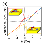
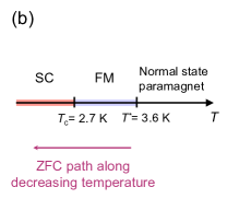
Figure 1: (a) A reproduction of the hysteresis curve from the magnetometry experiment Persky et al. (2022). The vertical axis counts the number of spontaneous vortices, and the horizontal axis is the training field applied above $T_{c}$; the insets illustrate the spontaneous vortices. (b) A heuristic phase diagram along the temperature axis inferred from the training-ZFC process. The magenta arrow defines the ZFC path.

In this paper we investigate a mechanism for the magnetic memory observed in the superconducting state that is consistent with the structure and symmetry of 4Hb-TaS₂. As a starting point, we assume that the metallic state above $T_{c}$ hosts at least a weak ferromagnetic (FM) moment, which may be too small to be detected (see Fig.  1(b)). We then determine the superconducting instabilities consistent with such a normal state and examine the requirements on the SC states for enhanced magnetization. Our key insight is that, the TRSB order, while suppressing the intralayer conventional BCS pairing, may favor an interlayer equal-spin pairing state protected by inversion symmetry. An imbalance between the spin-up and down pairings generically happens in this pairing state, such that the minority spin component can remain in an unpaired normal state. The angular momentum carried by the majority Cooper pairs gives rise to enhanced magnetization in the SC phase. The proposed mechanism leads to a number of predictions including a spin dependent “partial gap” structure, a linear-in-temperature specific heat, and the possibility of a second transition temperature below $T_{c}$, all of which are consistent with existing experiments Ribak et al. (2020); Nayak et al. (2021) or testable in the future.

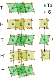
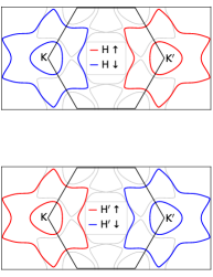
Figure 2: Left: Lattice structure of 4Hb-TaS₂. The tantulum (Ta) atoms form a simple stacking of triangular lattices with a four-layer-periodic unit cell $\mathrm{T}$–$\mathrm{H}$–$\mathrm{T}$–$\mathrm{H^{\prime}}$, where $\mathrm{T}$ and $\mathrm{H}$ denote two different layer structures. Right: FSs for the H layer (upper panel) and the $\mathrm{H^{\prime}}$ layer (lower panel). There are a smaller, near circular, hole-like FS and a larger, hexagonal, electron-like FS, concentered at the corners of the BZs, $\mathrm{K}$ and $\mathrm{K}^{\prime}$. Red and blue denote the spin-up and spin-down FSs centered at the BZ corners, respectively. The complete set of FSs consists all those in red, blue and gray.

Lattice structure and model.—The bulk 4Hb-TaS₂ structure is shown in Fig. 2. The lattice is centrosymmetric, with inversion centers residing on Ta atoms in the $\mathrm{T}$ layer. The inversion $i$ interchanges the $\mathrm{H}$ and $\mathrm{H^{\prime}}$ layers, and as we will show later, this fact is crucial to the formation of interlayer superconductivity. ARPES data Ribak et al. (2020) suggests that the bands near the Fermi energy come from the H and $\mathrm{H^{\prime}}$ layers and consist of three orbitals $d_{z^{2}}$, $d_{x^{2}-y^{2}}$, $d_{xy}$ and two spins $\sigma\!=\uparrow,\downarrow$ Liu et al. (2013). In this orbital subspace the dominant spin–orbit coupling (SOC) is the spin $S_{z}$-preserving Ising SOC $\hat{L}_{z}\hat{S}_{z}$. For all our microscopic calculations, we employ a six-band tight-binding model Not that matches DFT calculations Margalit et al. (2021) and ARPES data Ribak et al. (2020).

Magnetization in the normal state.— The ability to train the vortex state using a field below $T^{*}\!=\!3.6$ K implies a TRSB order with a spontaneous magnetization in the normal state. Here we leave open the microscopic origin of this TRSB order, but assume that the corresponding TRSB order parameter, $\phi$, couples to the electron spins as a Zeeman field. In addition to spin polarization, this coupling leads to orbital magnetization in the form of bond currents through the Ising SOC. We expect that the TRSB order has multiple frozen FM domains with random orientations, which get realigned by the training field below $T^{*}$. Below we estimate the magnetization of these aligned domains and discuss under which conditions it may be very small in the normal state and amplified below $T_{c}$.

Since we assumed that $\phi$ couples to the electrons as a Zeeman field, we introduce an effective field $B_{\text{eff}}$ to measure the splitting between the spin-up and -down bands: $E_{\uparrow}-E_{\downarrow}\simeq\phi\simeq\mu_{B}B_{\text{eff}}$. The total spontaneous magnetization $M^{z}_{\text{tot}}$ induced by $\phi$ (or equivalently, $B_{\text{eff}}$) is Not

$$M^{z}_{\text{tot}}=2.4\,\mathsf{B}_{\text{eff}}\times 10^{-4}\mu_{B}/V_{\text{u.c.}},$$ (1)

where $\mathsf{B}_{\text{eff}}$ is the numerical value of the effective chiral field $B_{\text{eff}}$ in Tesla (T), and $\mu_{B}/V_{\text{u.c.}}$ denotes Bohr magneton per volume of the four-layer unit cell $V_{\text{u.c.}}$. This provides an estimation of the strength of the weak FM order: for the magnetization in the TRSB phase to be non-detectable by a magnetometry device of sensitivity $10^{-10}$ T web , the order parameter (measured in Tesla) cannot exceed $B_{\text{eff}}=6\times 10^{-5}$ T.

Interlayer pairing. As the resistivity near the transition temperature exhibits BCS behavior with no substantial fluctuation regime Ribak et al. (2020), we here seek a pairing state consistent with a weak coupling BCS instability. This pairing is highly constrained by the Fermi surface (FS) geometry and symmetry. To see this, it is convenient to treat the layer index ($\mathrm{H},\mathrm{H^{\prime}}$) as a good quantum number. The essential physics, however, depends only on the lattice symmetry and does not change if we add interlayer hopping Not . The $(\uparrow,\mathrm{H})$ sector has a smaller, near circular, hole-like FS and a larger, hexagonal, electron-like FS, concentered at the $\mathrm{K}$ point of the $\mathrm{H}$-layer Brillouin zone (BZ). The $(\downarrow,\mathrm{H^{\prime}})$ sector has similar FSs centered at valley $\mathrm{K}$ of the $\mathrm{H^{\prime}}$-layer BZ, as shown in the right panel of Fig. 2. The FSs from the two sectors exactly coincide with each other. Similarly, the other two sectors, $(\uparrow,\mathrm{H}^{\prime})$ and $(\downarrow,\mathrm{H})$ have FSs centered at $\mathrm{K}^{\prime}$.

This FS geometry suggests that the only two possible pairing channels are

$$\underbrace{(\uparrow,\mathrm{H},\bm{k})\leftrightarrow(\downarrow,\mathrm{H},-\bm{k})}_{\text{opposite spin, intralayer}}\text{ or }\,\underbrace{(\uparrow,\mathrm{H},\bm{k})\leftrightarrow(\uparrow,\mathrm{H}^{\prime},-\bm{k})}_{\text{equal spin, interlayer}}.$$ (2)

The first channel in Eq. (2) describes the TRS-preserving, conventional BCS pairing. This channel is suppressed by the breaking of TRS in the normal state: the chemical potentials are different for the up and down spins, $E_{\uparrow}-E_{\downarrow}\neq 0$, and time-reversed electronic states are already energetically detuned, disfavoring the spin-singlet BCS pairing. On the other hand, the latter in (2) describes an inversion-symmetric, spin-triplet pairing, which remains a good pairing channel since the inversion symmetry is unbroken in the TRSB normal state. This is a simple argument in favor of interlayer superconductivity in 4Hb-TaS₂.

Furthermore, we argue that fluctuations of the TRSB order parameter can mediate this pairing. The effective action that couples the order parameter fluctuations to the low-energy electrons is $S=\chi^{-1}\phi^{2}\!+\!\phi(n_{\mathrm{H},\uparrow}\!-\!n_{\mathrm{H},\downarrow}\!+\!n_{\mathrm{H^{\prime}},\uparrow}\!-\!n_{\mathrm{H^{\prime}},\downarrow})$, where $\chi>0$ is the TRSB susceptibility. Upon integrating out $\phi$ one gets $S_{\text{eff}}\sim\!-\!\chi(n_{\mathrm{H},\uparrow}\!-\!n_{\mathrm{H},\downarrow}\!+\!n_{\mathrm{H^{\prime}},\uparrow}\!-\!n_{\mathrm{H^{\prime}},\downarrow})^{2}$. It contains the term $-\chi n_{\mathrm{H},\uparrow}n_{\mathrm{H^{\prime}},\uparrow}$ which is attractive when decoupled in the spin-triplet intra-layer pairing channel. On the other hand it contains the term $\chi n_{\mathrm{H},\uparrow}n_{\mathrm{H},\downarrow}$ which is repulsive in the conventional BCS channel. Therefore the only possible pairing favored by the fluctuations of $\phi$ is the interlayer spin-triplet pairing.

Symmetry and topology of the interlayer pairing.— We now turn to characterize the proposed interlayer spin-triplet pairing states in terms of lattice symmetry. The paramagnetic normal state has the full lattice point group symmetry $D_{6h}$, and the FM order breaks $D_{6h}$ down to $C_{6h}$. The interlayer, equal-spin pairing is necessarily symmetric in the spin channel, hence the orbital wave function must be antisymmetric, living in the odd parity irreps of $C_{6h}$. Furthermore, the pairing is intrinsically 3D: denote $\Delta_{\mathrm{H}\mathrm{H^{\prime}}}$ ($\Delta_{\mathrm{H^{\prime}}\mathrm{H}}$) as the pairing between $\mathrm{H}$ ($\mathrm{H^{\prime}}$) and the adjacent $\mathrm{H^{\prime}}$ ($\mathrm{H}$) layer right above it, $\Delta_{\mathrm{H}\mathrm{H^{\prime}}}$ and $\Delta_{\mathrm{H^{\prime}}\mathrm{H}}$ are related by the twofold rotation $c_{2}$ in $C_{6h}$ (strictly speaking, the twofold screw). Depending on the eigenvalue of $c_{2}$ being $+1$ or $-1$, we have $\Delta_{\mathrm{H}\mathrm{H^{\prime}}}=+\Delta_{\mathrm{H^{\prime}}\mathrm{H}}$ or $\Delta_{\mathrm{H}\mathrm{H^{\prime}}}=-\Delta_{\mathrm{H^{\prime}}\mathrm{H}}$, and the gap has maximum amplitude (horizontal line node) on the $k_{z}=0$ or $k_{z}=\pi$ respectively ($k_{z}=\pi$ or $k_{z}=0$) plane in the 3D BZ Not . For simplicity of presentation, we discuss the case of a single bilayer below. In this case $\Delta_{\mathrm{H}\mathrm{H^{\prime}}}$ carries the irrep of $S_{6}$, generated by inversion and $c_{3}$, and is fully characterized by a function in the 2D momentum plane $\bm{k}=(k_{x},k_{y})$. The full 3D gap function can be easily recovered from $\Delta_{\mathrm{H}\mathrm{H^{\prime}}}$ on the $k_{z}$ plane of maximum gap.

Denote $\Delta_{\bm{k},\uparrow}\!=\!\langle c^{\dagger}_{\bm{k},\mathrm{H},\uparrow}c^{\dagger}_{-\bm{k},\mathrm{H^{\prime}},\uparrow}\rangle$ as the interlayer pairing order parameter between $\mathrm{H}$ and the adjacent $\mathrm{H^{\prime}}$ layer above it. Due to the breaking of TRS, all the irreps of $S_{6}$ become one dimensional and allow chiral ansatze in the equal-spin-up channels. Due to the discrete rotation $c_{3}$, the orbital angular momentum carried by $\Delta_{\bm{k},\uparrow}$ is defined modulo $3$; Equivalently, the gap windings on the inner and outer FSs centered at $\mathrm{K}$ can only differ by multiples of $6\pi$. Furthermore, this winding difference, or the total gap winding upon including the sign $+$/$-$ for electron-/hole-like FSs, exactly defines the (gauge invariant) Chern number $c_{\text{BdG}}$ for the Bogoliubov-de Gennes (BdG) bands. From this we conclude that the BdG Chern number can only be multiples of $3$.

To illustrate the principles of the above analysis, we perform a microscopic calculation by solving the BCS mean-field equation for the interlayer pairing gap function Not

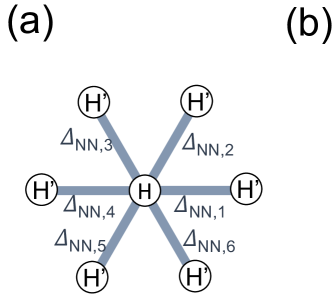
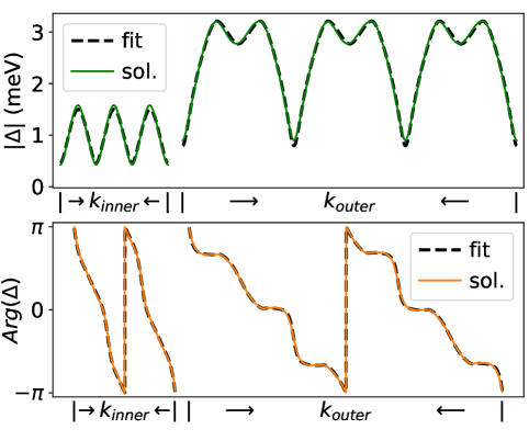
Figure 3: (a) Illustration of the real space, NN interlayer pairing between layers $\mathrm{H}$ and $\mathrm{H^{\prime}}$. (b) The gap function $\Delta$ for the $c_{\text{BdG}}=0$ ansatz. The upper (lower) panel shows the amplitude (phase) of $\Delta$ on both the inner and outer FSs. The solid lines are solved from the gap equation (3) and the dashed lines are obtained from a NN interlayer pairing ansatz as a lattice approximation. The gap minimum is normalized to the experimental gap size $0.44$ meV Nayak et al. (2021).

$$\Delta_{\bm{k},\uparrow}\!=\!-\!\int\!\frac{d^{2}\!k^{\prime}}{(\!2\pi\!)^{2}}V_{\bm{k}-\bm{k}^{\prime}}\!\langle u_{\bm{k},\uparrow,\mathrm{H}}|u_{\bm{k}^{\prime},\uparrow,\mathrm{H}}\rangle^{\!2}\frac{\tanh\!\frac{\varepsilon_{\bm{k}^{\prime}}}{2T}}{2\varepsilon_{\bm{k}^{\prime}}}\Delta_{\bm{k}^{\prime},\uparrow},$$ (3)

here $|u_{\bm{k},\uparrow,\mathrm{H}}\rangle$ is the normal state Bloch wave function for spin $\uparrow$ and layer $\mathrm{H}$, $\varepsilon_{\bm{k}}$ is the dispersion of the Bogoliubov quasi-particles, and we assumed for simplicity a constant attractive interaction $V_{\bm{k}}\!=\!V\!<\!0$. The solution is shown in Fig. 3(b). This ansatz lives in the $E_{u}$ irrep of $S_{6}$ and has a $-4\pi$ winding on both the inner and outer FSs, but has a vanishing Chern number, $c_{\text{BdG}}\!=\!0$ Not .

Unpaired minority component.— A direct consequence of the interlayer spin-polarized pairing we have described is that the other spin component remains unpaired and forms a gapless Fermi surface below $T_{c}$. This can be understood from a Landau free energy analysis. Denote the real space, coarse grained interlayer spin-polarized pairing order parameters as $\Delta_{\sigma}$. At quadratic level the allowed terms are $F_{2}=\sum_{\sigma}r_{\sigma}|\Delta_{\sigma}|^{2}$, where $r_{\uparrow}$ and $r_{\downarrow}$ are in general different because time reversal symmetry is already broken in the normal state. As a consequence the critical temperatures for pairing of the two spin components $T_{c\uparrow}$ and $T_{c\downarrow}$ are also different. Note that there is no proximity coupling between the paired and unpaired components because the cross term $\Delta_{\uparrow}\Delta_{\downarrow}^{*}$ is forbidden due to spin ($S_{z}$) conservation. Therefore the unpaired spin component remains gapless and forms a Fermi liquid between the upper and lower critical temperatures.

The prediction of two transition temperatures raises a possible disrepancy between this theory and experimental observations. Since the breaking of TRS in the normal state is assumed to be weak, one might expect it would lead to only a small difference between the two critical temperatures. However, experiments have not observed the lower transition temperature down to at least $0.5$ K Ribak et al. (2020); van . The discrepancy may be resolved by considering the quartic terms of the Landau energy: $F_{4}=u(|\Delta_{\uparrow}|^{4}+|\Delta_{\downarrow}|^{4})+v|\Delta_{\uparrow}|^{2}|\Delta_{\downarrow}|^{2}$. While the coefficient $u$ is a property of the electronic band structure, the other coefficient $v\propto\chi^{2}$ is proportional to the square of the chiral susceptibility $\chi$ Not . When the fluctuations of $\phi$ are sufficiently strong such that $v\!>\!2u\!>\!0$, a total suppression of the minority spin pairing can be achieved.

Magnetization in the superconducting state.— Having discussed general features of the interlayer pairing states we now come to the central discussion of how and to what extent such pairing amplifies the normal state magnetization. To this end, we derive in Not expressions for spin and orbital magnetizations in the interlayer pairing state. Importantly, the orbital magnetization explicitly contains a Berry curvature contribution, which traces back to the orbital angular momentum of the pairing state (A similar relation is known for the normal state orbital magnetization Shi et al. (2007)). One consequence is that a nonzero $c_{\text{BdG}}$ enhances orbital magnetization, as we will show in detail below.

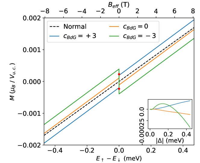
Figure 4: Magnetization in the normal state (dashed black line) and in the interlayer pairing ansatze (solid lines) with a gapsize of 0.44 meV. The three pairing ansatze have BdG Chern numbers $+3$ (blue), $0$ (orange) and $-3$ (green). The lower and upper horizontal axes are related by $E_{\uparrow}-E_{\downarrow}=\mu_{\text{B}}B_{\text{eff}}$ (see the discussion above Eq. (1)). The two red dots denote the remnant magnetization inferred from the experiment Persky et al. (2022). The inset shows the magnetization as a function of the gap size for the three pairing ansatze. Magnetizations are all calculated at $T=2$ K.

We use the derived magnetization formula to calculate the magnetization in various inter-layer pairing states consistent with the lattice symmetry. The simplest ansatze with pairing along a vertical bond between $\mathrm{H}$ and $\mathrm{H}^{\prime}$ Nno always give zero BdG Chern number. As we will be focusing on examining the relation between magnetization and $c_{\text{BdG}}$, we would like to obtain ansatze with nonzero Chern numbers of $\pm 3$. To find them, we consider ansatze with nonzero nearest-neighbor (NN) interlayer pairing as sketched in Fig. 3(a). Furthermore, we construct a NN ansatz that gives good approximation to the $c_{\text{BdG}}=0$ gap solution of Eq. (3), see Fig. 3(b). We thus obtain three ansatze with distinct Chern numbers $c_{\text{BdG}}=0,\pm 3$, whose form and the computed magnetizations can be found in Not . Below we present the magnetization result for these three ansatze.

In Fig. 4 we plot the magnetization as a function of the effective Zeeman energy splitting $E_{\uparrow}-E_{\downarrow}$ induced by the TRSB order parameter $\phi$ for the three NN ansatze mentioned above. All three exhibit a jump in the magnetization $\Delta M$ when $E_{\uparrow}-E_{\downarrow}$ crosses zero. Only the $c_{\text{BdG}}=+3$ state gives a positive, paramagnetic jump in magnetization, while both the $c_{\text{BdG}}=0,-3$ ansatze give a negative (diamagnetic) jump. Comparison with the experimental hysteresis curve in Fig. 1 points at the $c_{\text{BdG}}\!=\!+3$ ansatz as being the most promising candidate state of the three ansatze. Encouragingly, the magnitude of the jump is also found to be of the same order of magnitude as the remnant field deduced experimentally, $M_{\text{SC,exp}}\!=\!2.28\times 10^{-4}\mu_{\text{B}}/V_{\text{u.c.}}$ (red dots in Fig. 4) Persky et al. (2022).

Further remarks on magnetization are in order. We notice from Fig. 4 that the size of the hysteresis jump is approximately proportional to $c_{\text{BdG}}$, consistent with the understanding that a nonzero $c_{\text{BdG}}$ enhances the orbital magnetization, and further suggests that the orbital magnetization is the leading contribution to the total magnetization. However, we point out that the precise relation between the gap winding and the magnetization is not straightforward, as several factors (such as the gap sizes on the inner and outer FSs and temperature) can affect the magnetization, even for a given gap winding. As an illustration to this caveat, we plot in the inset of Fig. 4 the magnetization as a function of gap size at an infinitesimal field, and point out that the $c_{\text{BdG}}=-3$ ansatz can still have a positive magnetization at very small gap size. Nevertheless, for the experimentally relevant temperature and gap size, the orbital magnetization is the leading contribution for large gap winding and the expected relation between the total gap winding and hysteresis jump holds Not . Combining the numerical results of $c_{\text{BdG}}$ and magnetization, we present the following picture for understanding the experimental observations on 4Hb-TaS₂: if the $1\mathrm{H}$ and $1\mathrm{H^{\prime}}$ layers are in an interlayer spin-triplet pairing state with $c_{\text{BdG}}=3$, and a large imbalance between the number of spin-up and spin-down Cooper pairs exists, an amplified magnetization can appear due to the excessive angular momentum carried by the majority spin Cooper pair.

Discussion.—In conclusion, we have formulated a phenomenological theory to understand the puzzling appearance of spontaneous vortices in 4Hb-TaS₂. Assuming that a weak FM order develops in the normal state, we showed that a weak coupling BCS instability exists in the interlayer, spin-polarized pairing channel. The breaking of TRS results in imbalance in the spin-up and spin-down pairings, and a total suppression of the minority spin pairing may be achieved, consistent with a single $T_{c}$ observed in experiment. The angular momentum carried by the majority spin Cooper pair naturally enhances the magnetization and explains the appearance of spontaneous vortices in the SC phase. Our proposal of interlayer, spin-polarized pairing in a single spin component for 4Hb-TaS₂ is quite different from previous proposals Margalit et al. (2021); Dentelski et al. (2021); König (2023). Our proposed pairing state can be verified in a spin-polarized scanning tunneling microscopy (STM) experiment Wang et al. (2021), in which a gap should be observed only in one spin component, but not in the other. We note that such a “partial gap” structure has been observed in a previous (spin-unpolarized) STM experiment Ref. Nayak et al. (2021). More generally, our theory suggests a novel kind of FM superconductor and could be relevant to a large family of centrosymmetric compounds Fischer et al. (2022).

Finally, we mention a few predictions of our theory for existing and potential future experiments. First, we note that the superconducting temperature $T_{c}=2.7$ K is consistently reported in all experiments with or without a field training. It is plausible that the superconductivity in 4Hb-TaS₂ reported so far are all preceded by a TRSB state at higher temperature, and the existence of multiple randomly oriented domains prohibits macroscopic ferromagnetism, hence the lack of observation of magnetic moment in the normal state. Second, in our proposed pairing state, the unpaired minority Fermi surface exhibits a linear-in-temperature specific heat, in agreement with the measured temperature scaling of specific heat Ribak et al. (2020). We note that the specific heat reveals a $\sim 15\%$ residual contribution in the SC state Ribak et al. (2020) and two distinct superconducting transitions are not observed down to $0.5$ K. While these are not quantitatively explained by our current theory, we pointed out the possibility that superconductivity of the majority spin-species can promote enhanced fluctuations or pseudogap-like behavior for the minority spin-species. The detailed investigation of such suppression of gapless excitations is left for future work. Third, we have not pointed towards any specific microscopic origin for the TRSB order parameter $\phi$. While the most natural interpretation for $\phi$ is a FM order parameter, other scenarios are also possible, in which $\phi$ is the scalar spin chirality in a chiral U(1) spin liquid Persky et al. (2022). The microscopic mechanism that leads to the TRSB metallic phase is an interesting question for future theory and experiments.

Acknowledgements—We thank J. E. Moore, Z. Dai, Y.-P. Lin, and H. Beidenkopf for helpful discussions. This research was supported by the Gordon and Betty Moore Foundation (C.L.) and a Simons Investigator award (E.A.). S.C. was supported by the ARO through the MURI program (grant number W911NF17-1-0323). E.B. acknowledges support from the European Research Council (ERC) under grant HQMAT (grant agreement No. 817799), and the hospitality of the Aspen Center for Physics, supported by National Science Foundation grant PHY-2210452, where part of this work was done.

Supplementary Material for "Magnetization amplification in the interlayer pairing superconductor 4Hb-TaS₂"

Appendix A interlayer pairing mechanism and phase diagram

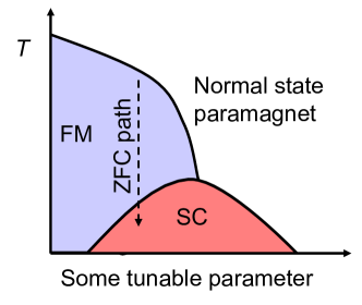
Figure S1: Conjectured 2D phase diagram for 4Hb-TaS₂.

In the main text we proposed a mechanism for the interlayer spin-triplet pairing mediated by the fluctuation of the TRSB/FM order parameter $\phi$. The underlying assumption for this mechanism is a two dimensional phase diagram spanned by temperature and another tunable parameter (such as doping, strain etc.), as shown in Fig. S1. We assume that a quantum phase transition entering the FM phase happens at $T=0$ as the the horizontal axis parameter is tuned, around which the quantum fluctuation of the FM order is large; such a phase transition is hidden inside the dome of the SC phase. As a result, fluctuations of the order parameter $\phi$ may still be strong as one approaches along a low temperature horizontal path from the paramagnetic phase to the ferromagnetic phase. This path is distinct from the vertical, ZFC path traced out in the experiment, on which a FM order establishes at higher temperature and the fluctuation of $\phi$ in the FM phase is small.

Appendix B Lattice symmetry

We set up the coordinates in such a way that $x$ axis is parallel to the bond $R_{1}$ in Fig. S2. Denote the lattice constant (i.e. the nearest neighbor bond distance) to be $a$. The origin is placed on an inversion center on the 1T layer. The $z$ periodicity is four layers (1H’-1T-1H-1T), with a four-layer distance $c$. We have $a=3.3381\text{ \AA}$ and $c=23.728\text{ \AA}$ Ribak et al. (2020). 4Hb-TaS₂ has No. 194 space group $P6_{3}/mmc$, and the point group is $D_{6h}$ of order 24, generated by

$$D_{6h}=\langle m_{z},m_{x},i,c_{3}\rangle=\langle m_{x},i,s_{2},c_{3}\rangle,$$ (S1)

where

$$m_{z} \colon\quad(x,y,z)\rightarrow(x,y,\pm\frac{1}{2}-z),$$ (S2a)

$$m_{x} \colon\quad(x,y,z)\rightarrow(-x,y,z),$$ (S2b)

$$i \colon\quad(x,y,z)\rightarrow(-x,-y,-z),$$ (S2c)

$$s_{2} \colon\quad(x,y,z)\rightarrow(-x,-y,z+1/2),$$ (S2d)

$$c_{3} \colon\quad(x,y,z)\rightarrow\Big{(}-\frac{x}{2}-\frac{\sqrt{3}}{2}y,\frac{\sqrt{3}}{2}x-\frac{1}{2}y,z\Big{)},$$ (S2e)

here, $i$ is inversion about an Ta atom on the 1T layer; $m_{z}$ is reflection along $z$, with the mirror plane either the 1$\mathrm{H}$ or the 1$\mathrm{H^{\prime}}$ layer; $m_{x}$ is reflection along $x$; $s_{2}$ is a two-fold screw along $z$, and $c_{3z}$ is a threefold rotation along $z$. Note we have $m_{z}=is_{2}$, $s_{2}=m_{z}i$ up to translations. Abstractly, we have $D_{6h}\cong Dih_{6}\times Z_{2}\cong Dih_{3}\times Z_{2}^{2}$. It is easy to see that $i$ commutes with all other elements. On the other hand, it is clear that $m_{x}$ does not commute with $c_{3}$. Therefore $Dih_{3}=\langle c_{3},m_{x}\rangle$, and $\mathbb{Z}_{2}^{2}=\langle s_{2}\rangle\times\langle i\rangle$.

A few comments: (1) a single layer structure (1H-TaS₂) has point group symmetry $D_{3h}=\langle m_{x},m_{z},c_{3}\rangle$ which has 12 element. (2) a bilayer (2H-TaS₂) structure has point group symmetry $\langle m_{x},i,c_{3}\rangle$, where the inversion $i$ is centered between the two layers. (3) In bulk 4Hb-TaS₂, the 1T layer is not a mirror plane.

Appendix C Tight binding Hamiltonian for the normal state

The tight binding Hamiltonian is constructed in the same way as Ref. Margalit et al. (2021), which we present here for completeness. The bands near the Fermi surface is mainly contributed by three orbitals $d_{z^{2}}$, $d_{x^{2}-y^{2}}$, and $d_{xy}$. In angular momentum basis $|l,m\rangle$ we have $|d_{z^{2}}\rangle=|2,0\rangle$, $|d_{x^{2}-y^{2}}\rangle=\frac{1}{\sqrt{2}}(|2,2\rangle+|2,-2\rangle)$ and $|d_{xy}\rangle=-\frac{i}{\sqrt{2}}(|2,2\rangle-|2,-2\rangle)$. The angular momentum operators in this orbital subspace have the form

$$\hat{L}_{z}=\left(|d_{z^{2}}\rangle,|d_{xy}\rangle,|d_{x^{2}-y^{2}}\rangle\right)\underbrace{\left(\begin{array}[]{ccc}0&0&0\\ 0&0&2i\\ 0&-2i&0\end{array}\right)}_{L_{z}}\left(\begin{array}[]{c}\langle d_{z^{2}}|\\ \langle d_{xy}|\\ \langle d_{x^{2}-y^{2}}|\end{array}\right),\qquad\hat{L}_{x}=\hat{L}_{y}=0.$$ (S3)

The nearest, second nearest and third nearest hopping matrix are constrained by lattice symmetry to have the form

$$R_{1}=\left(\begin{array}[]{ccc}t_{0}&-t_{1}&t_{2}\\ t_{1}&t_{11}&-t_{12}\\ t_{2}&t_{12}&t_{22}\end{array}\right),\quad S_{1}=\left(\begin{array}[]{ccc}r_{0}&r_{2}&-\frac{r_{2}}{\sqrt{3}}\\ r_{1}&r_{11}&r_{12}\\ -\frac{r_{1}}{\sqrt{3}}&r_{12}&\left(r_{11}+\frac{2}{\sqrt{3}}r_{12}\right)\end{array}\right),\quad T_{1}=\left(\begin{array}[]{ccc}u_{0}&-u_{1}&u_{2}\\ u_{1}&u_{11}&-u_{12}\\ u_{2}&u_{12}&u_{22}\end{array}\right).$$ (S4)

We have

$$Q_{3}=\mathbf{R}^{T}Q_{1}\mathbf{R},\quad Q_{5}=\mathbf{R}Q_{1}\mathbf{R}^{T},\quad Q_{4}=Q_{1}^{\dagger},\quad Q_{6}=\mathbf{R}^{T}Q^{\dagger}_{1}\mathbf{R},\quad Q_{2}=\mathbf{R}Q^{\dagger}_{1}\mathbf{R}^{T},$$ (S5)

where

$$\mathbf{R}\equiv\mathbf{R}(2\pi/3\hat{z})\equiv e^{-i\frac{2\pi}{3}L_{z}}\equiv\begin{pmatrix}1&&\\ &-1/2&-\sqrt{3}/2\\ &\sqrt{3}/2&-1/2\end{pmatrix}$$ (S6)

is the unitary matrix for the three-fold rotation $c_{3}$, and $Q_{i}=R_{i},S_{i},T_{i}$ ($i=1,2,...,6$) denote the nearest, second-nearest and third-nearest neighbor hopping matrices, respectively.

The tight binding parameters in units of meV are, following Refs. Möckli and Khodas (2018); Margalit et al. (2021),

$$(t_{0},t_{1},t_{2},t_{11},t_{12},t_{22}) =(-0.1917,0.4057,0.4367,0.2739,0.3608,-0.1845),$$ (S7)

$$(r_{0},r_{1},r_{2},r_{11},r_{12},r_{22}) =(0.0409,-0.069,0.0928,-0.0066,0.1116,0),$$

$$(u_{0},u_{1},u_{2},u_{11},u_{12},u_{22}) =(0.0405,-0.0324,-0.0141,0.1205,-0.0316,-0.0778),$$

$$(\epsilon_{0},\epsilon_{1},\epsilon_{2},\mu_{0},\lambda_{\text{SO}}) =(1.6507,2.5703,2.5703,-0.0500,0.1713).$$

The orbital basis in real space is defined as

$$d^{\dagger}_{\bm{r},\mathrm{H}}=\left(d^{\dagger}_{z^{2},\uparrow,\bm{r},\mathrm{H}},d^{\dagger}_{xy,\uparrow,\bm{r},\mathrm{H}},d^{\dagger}_{x^{2}-y^{2},\uparrow,\bm{r},\mathrm{H}},d^{\dagger}_{z^{2},\downarrow,\bm{r},\mathrm{H}},d^{\dagger}_{xy,\downarrow,\bm{r},\mathrm{H}},d^{\dagger}_{x^{2}-y^{2},\downarrow,\bm{r},\mathrm{H}}\right),$$ (S8)

where $\bm{r}$ labels sites on one layer. After Fourier transform $d^{\dagger}_{\bm{k},\mathrm{H}}=\frac{1}{\sqrt{N}}\sum_{\bm{r}}e^{i\bm{k}\cdot\bm{r}}d^{\dagger}_{\bm{r},\mathrm{H}}$ we have the Hamiltonian for the $\mathrm{H}$ layer:

$$H_{\text{H}}=\sum_{\bm{k}}d^{\dagger}_{\bm{k},\mathrm{H}}\mathcal{H}_{\mathrm{H}}(\bm{k})d_{\bm{k},\mathrm{H}}$$ (S9)

with

$$\mathcal{H}_{\mathrm{H}}(\bm{k})=E+\sigma_{0}\otimes\left(\sum_{i=1}^{6}R_{i}e^{i\bm{R}_{i}\cdot\bm{k}}+S_{i}e^{i\bm{S}_{i}\cdot\bm{k}}+T_{i}e^{i\bm{T}_{i}\cdot\bm{k}}\right),$$ (S10)

where the onsite term is $E=\sigma_{0}\otimes\text{diag}(\epsilon_{0}-\mu_{0},\epsilon_{1}-\mu_{0},\epsilon_{2}-\mu_{0})+\frac{\lambda_{\text{SO}}}{2}\sigma_{z}\otimes L_{z}$. Diagonalizing $H_{\mathrm{H}}$ gives

$$H_{\mathrm{H}}=\sum_{n,\sigma}E_{n,\sigma,\bm{k}}c^{\dagger}_{n,\sigma,\bm{k}}c_{n,\sigma,\bm{k}},$$ (S11)

where $n=1,2,3$ labels the band for one spin sector $\sigma$, $c_{n,\sigma,\bm{k}}=\sum_{\ell}\big{(}u^{(\ell)}_{n,\sigma,\bm{k}}\big{)}^{*}d_{\ell,\sigma,\bm{k},\mathrm{H}}$, here $\ell=z^{2},xy,x^{2}-y^{2}$ labels the orbitals, and $u^{(\ell)}_{n,\sigma,\bm{k}}$ is the $\ell$-th component of the eigenvector $u_{n,\sigma,\bm{k}}$ satisfying $\mathcal{H}_{\mathrm{H}}(\bm{k})u_{n,\sigma,\bm{k},\mathrm{H}}=E_{n,\sigma,\bm{k}}u_{n,\sigma,\bm{k},\mathrm{H}}$ with energy eigenvalues given by $E_{n,\sigma,\bm{k}}$. The dispersion is shown in Fig. S2.

Now we have $c_{3}\colon d_{\bm{k}}\rightarrow e^{-i\frac{2\pi}{3}L_{z}}e^{-i\frac{\pi}{3}\sigma}d_{c_{3}(\bm{k})}=e^{-i\frac{\pi}{3}\sigma}\mathbf{R}d_{c_{3}(\bm{k})}$, and we choose the gauge such that $u_{n\bm{k}}=\mathbf{R}u_{n,c_{3}(\bm{k})}$, therefore

$$c_{3}\colon c_{n\bm{k}}\rightarrow e^{-i\frac{\pi}{3}\sigma}c_{n,c_{3}(\bm{k})}.$$ (S12)

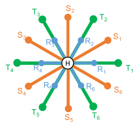
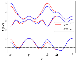
Figure S2: Tight binding model for 1H-TaS₂. Left: definition of the nearest, 2nd-nearest, and 3rd-nearest neighbor bonds within the $\mathrm{H}layer$. Right: Energy dispersion along high symmetry path in the Brillouin zone.

Symmetry action on the tight-binding Hamiltonian in momentum space gives

$$m_{z} \colon U^{\dagger}_{m_{z}}\mathcal{H}_{\mathrm{H}}(\bm{k})U_{m_{z}}=\mathcal{H}_{\mathrm{H}}(\bm{k}),$$ (S13a)

$$m_{x} \colon U^{\dagger}_{m_{x}}\mathcal{H}_{\mathrm{H}}(-k_{x},k_{y})U_{m_{x}}=\mathcal{H}_{\mathrm{H}}(\bm{k}),$$ (S13b)

$$i \colon U^{\dagger}_{i}\mathcal{H}_{\mathrm{H}}(-\bm{k})U_{i}=\mathcal{H}_{\mathrm{H}}(\bm{k}),$$ (S13c)

$$c_{3} \colon U^{\dagger}_{c_{3}}\mathcal{H}_{\mathrm{H}}(c_{3}^{-1}(\bm{k}))U_{c_{3}}=\mathcal{H}_{\mathrm{H}}(\bm{k}),$$ (S13d)

$$\mathcal{T} \colon\sigma^{y}\mathcal{H}_{\mathrm{H}}^{*}(-\bm{k})\sigma^{y}=\mathcal{H}_{\mathrm{H}}(\bm{k}),$$ (S13e)

where

$$U_{m_{z}} =(-i\sigma^{z})\otimes 1_{3\times 3},$$ (S14a)

$$U_{m_{x}} =(-i\sigma^{x})\otimes\mathrm{diag}(1,-1,1),$$ (S14b)

$$U_{i} =1_{2\times 2}\otimes 1_{3\times 3},$$ (S14c)

$$U_{c_{3}} =e^{-i\frac{\pi}{3}\sigma^{z}}\otimes\mathbf{R},$$ (S14d)

$$U_{\mathcal{T}} =i\sigma^{y}\otimes\mathcal{K}1_{3\times 3},$$ (S14e)

the mirror $m_{z}$ forbids Rashba spin-orbit coupling. As a consequence, the spin-up and spin-down sectors are decoupled, and the energy bands are labeled by $(n,\sigma)$ with $n=1,2,3$ and $\sigma=\uparrow,\downarrow$.

Finally, the $\mathrm{H}$ and $\mathrm{H^{\prime}}$ are related by the inversion $i$:

$$\mathcal{H}_{\mathrm{H}^{\prime}}(\bm{k})=\mathcal{H}_{\mathrm{H}}(-\bm{k}).$$ (S15)

Appendix D BdG Hamiltonian

Now we analyze the pairing in real space. We assume equal spin, interlayer pairing, i.e. the pairing is only between the same spin species of the $\mathrm{H}$ layer and the $\mathrm{H}^{\prime}$ layer. For the rest of this section, we will focus on the spin up sector and quite often we will omit the spin index $\sigma=\uparrow$.

$$H_{\text{pairing},\uparrow}=\sum_{\bm{r},\bm{\delta}}(d^{\dagger}_{z^{2},\uparrow,\bm{r},\mathrm{H}},d^{\dagger}_{xy,\uparrow,\bm{r},\mathrm{H}},d^{\dagger}_{x^{2}-y^{2},\uparrow,\bm{r},\mathrm{H}})\Delta_{\bm{\delta}}\left(\begin{array}[]{c}d^{\dagger}_{z^{2},\uparrow,\bm{r}+\bm{\delta},\mathrm{H}^{\prime}}\\ d^{\dagger}_{xy,\uparrow,\bm{r}+\bm{\delta},\mathrm{H}^{\prime}}\\ d^{\dagger}_{x^{2}-y^{2},\uparrow,\bm{r}+\bm{\delta},\mathrm{H}^{\prime}}\end{array}\right)+h.c.,$$ (S16)

where $\Delta_{\bm{\delta}}$ is a $3\times 3$ matrix denoting the $\bm{\delta}$-neighbor pairing in the orbital space. We model $\Delta_{\bm{\delta}}$ phenomenologically by the following Ansatz

$$\Delta^{\text{onsite}}_{\bm{\delta}=0}=0_{3\times 3},\qquad\Delta^{\text{NN}}_{\bm{\delta}=a\hat{x}}=[\Delta_{1}]_{i,j=1}^{3},\qquad\Delta^{\text{NN}}_{\bm{\delta}=-a\hat{x}}=[\Delta_{2}]_{i,j=1}^{3},$$ (S17)

and the other four nearest-neighbor pairing matrices are related to $\Delta^{\text{NN}}_{\bm{\delta}=\pm a\hat{x}}$ by

$$\Delta^{\text{NN}}_{\bm{\delta}=(\frac{\hat{x}}{2}-\frac{\sqrt{3}}{2}\hat{y})a}=e^{i\frac{2\pi}{3}}\mathbf{R}^{T}\Delta^{\text{NN}}_{\bm{\delta}=-a\hat{x}}\mathbf{R},\qquad\Delta^{\text{NN}}_{\bm{\delta}=(\frac{\hat{x}}{2}+\frac{\sqrt{3}}{2}\hat{y})a}=e^{-i\frac{2\pi}{3}}\mathbf{R}\Delta^{\text{NN}}_{\bm{\delta}=-a\hat{x}}\mathbf{R}^{T},$$ (S18)

$$\Delta^{\text{NN}}_{\bm{\delta}=(-\frac{\hat{x}}{2}+\frac{\sqrt{3}}{2}\hat{y})a}=e^{i\frac{2\pi}{3}}\mathbf{R}^{T}\Delta^{\text{NN}}_{\bm{\delta}=a\hat{x}}\mathbf{R},\qquad\Delta^{\text{NN}}_{\bm{\delta}=(-\frac{\hat{x}}{2}-\frac{\sqrt{3}}{2}\hat{y})a}=e^{-i\frac{2\pi}{3}}\mathbf{R}\Delta^{\text{NN}}_{\bm{\delta}=a\hat{x}}\mathbf{R}^{T}.$$

Two ansatze with only vertical pairing $\Delta^{\text{onsite}}_{\bm{\delta}=0}$ are given in App. E, see Eqs. (S38) and (S39).

In the main text (see Fig. 4), we consider the following three ansatze and their magnetization:

• A $c_{\text{BdG}}=0$ ansatz:

  $$\Delta_{1} =\left(\begin{array}[]{ccc}-0.0076+0.0097i&0&0\\ 0&-0.0350-0.0388i&-0.0333-0.0088i\\ 0&-0.0333-0.0088i&-0.0339+0.0182i,\end{array}\right),$$ (S19)

  $$\Delta_{2} =\left(\begin{array}[]{ccc}-0.00260-0.02070i&0&0\\ 0&-0.0227+0.0606i&0.0387-0.0176i\\ 0&0.0387-0.0176i&-0.0486-0.0169i\end{array}\right),$$

• A $c_{\text{BdG}}=3$ ansatz:

  $$\Delta_{1} =\left(\begin{array}[]{ccc}-0.9318-1.2584i&-0.8524-0.9916i&0.017-0.6868i\\ 0.8457-1.4012i&0.2481-0.203i&-0.5522-2.1722i\\ 0.3962-0.7074i&0.2016+1.5976i&0.4721+0.0654i\end{array}\right),$$ (S20)

  $$\Delta_{2} =\left(\begin{array}[]{ccc}0.3887-0.3335i&-1.0758+0.2915i&0.1068-1.1865i\\ -0.0022-0.7062i&1.0894+0.6527i&0.7976+1.9333j\\ -0.4683+1.4212i&0.089-0.1511i&-1.4346-0.9278i\end{array}\right)$$

• A $c_{\text{BdG}}=-3$ ansatz:

  $$\Delta_{1} =\left(\begin{array}[]{ccc}-0.5664+1.2343i&-0.0211+0.5998i&-0.9211+0.4951i\\ 0.5770+0.8565i&-0.0976+0.7141i&-0.4165-0.6214i\\ -0.4841+1.2828i&-2.1290-0.1987i&-0.01612-0.3777i\end{array}\right),$$ (S21)

  $$\Delta_{2} =\left(\begin{array}[]{ccc}-0.4466-0.0670i&1.4044-2.1840i&-0.3420-0.7554i\\ -0.6443+0.2467i&-0.4718+0.6550i&1.5598+1.1051i\\ 0.0210+0.2556i&-1.6399+0.3480i&-0.6115+1.6498i\end{array}\right)$$

The BdG Hamiltonian reads

$$H_{\text{BdG},\uparrow} =H_{\mathrm{H},\uparrow}+H_{\mathrm{H^{\prime}},\uparrow}+H_{\text{pairing},\uparrow}$$ (S22)

$$=\sum_{\bm{k}}(d^{\dagger}_{\bm{k},\uparrow,\mathrm{H}},d^{T}_{-\bm{k},\uparrow,\mathrm{H}^{\prime}})\underbrace{\left(\begin{array}[]{cc}\mathcal{H}_{\mathrm{H}}(\bm{k})&\Delta^{\text{orb}}(\bm{k})\\ \left(\Delta^{\text{orb}}(\bm{k})\right)^{\dagger}&-\mathcal{H}^{T}_{\mathrm{H}}(\bm{k})\end{array}\right)}_{\mathcal{H}_{\text{BdG}}(\bm{k})}\left(\begin{array}[]{c}d_{\bm{k},\uparrow,\mathrm{H}}\\ \big{(}d^{\dagger}_{-\bm{k},\uparrow,\mathrm{H}^{\prime}}\big{)}^{T}\end{array}\right),$$

where we defined the Hamiltonian matrix

$$\mathcal{H}_{\text{BdG}}(\bm{k})=\left(\begin{array}[]{cc}\mathcal{H}_{\mathrm{H}}(\bm{k})&\Delta^{\text{orb}}(\bm{k})\\ \left(\Delta^{\text{orb}}(\bm{k})\right)^{\dagger}&-\mathcal{H}^{T}_{\mathrm{H}}(\bm{k})\end{array}\right)$$ (S23)

where we have used the relation (S15). $\Delta^{\text{orb}}({\bm{k}})$ is the pairing matrix in momentum space which we keep only up to nearest-neighbor bonds and has the form

$$\Delta^{\text{orb}}({\bm{k}})=\Delta^{\text{onsite}}_{\bm{\delta}=0}+\sum_{i=1}^{6}\Delta^{\text{NN}}_{\bm{\delta}_{i}}e^{i\bm{k}\cdot\bm{\delta}_{i}},$$ (S24)

where $\bm{\delta}_{i}$ are the six nearest-neighbor bonds.

We project $\Delta^{\text{orb}}_{\bm{k}}$ to the lowest band to obtain the gap function of that band, $\Delta(\bm{k})$:

$$\Delta(\bm{k})\simeq\Delta^{\text{orb proj.}}_{\bm{k}}=u^{\dagger}_{\bm{k},\mathrm{H}}\Delta^{\text{orb}}(\bm{k})u^{*}_{-\bm{k},\mathrm{H}^{\prime}}=u^{\dagger}_{\bm{k},\mathrm{H}}\Delta^{\text{orb}}(\bm{k})u^{*}_{\bm{k},\mathrm{H}},$$ (S25)

where we have made use of the inversion symmetry for the normal state wave function $u_{\bm{k},\mathrm{H}}=u_{-\bm{k},\mathrm{H}^{\prime}}$ (see Eq. (S14c)). The relation (S25) established the connection between our effective theory and the microscopic orbital pairing in the lattice. The symmetry properties of the BdG Hamiltonian will be discussed in the next section.

Appendix E Pairing symmetry

E.1 A bilayer treatment

Here we discuss the symmetry classification of the gap function. Recall that normal state Hamiltonian $H_{0}$ preserves the full point group symmetry $D_{6h}=\langle c_{3},m_{x},m_{z},i\rangle$. Let $\sigma^{0,1,2,3}$ denote the Pauli matrices for the spin space $\uparrow,\downarrow$ and $\mu^{0,1,2,3}$ denote those for the layer space $\mathrm{H}$ and $\mathrm{H^{\prime}}$. The most general pairing is written as

$$H_{\text{pairng}}=\sum_{\bm{k}}c^{\dagger}_{\bm{k}}\Delta(\bm{k})(c^{\dagger}_{-\bm{k}})^{T},\quad\text{with}\quad c^{\dagger}_{\bm{k}}=(c^{\dagger}_{\bm{k},\uparrow,\mathrm{H}},c^{\dagger}_{\bm{k},\uparrow,\mathrm{H}^{\prime}},c^{\dagger}_{\bm{k},\downarrow,\mathrm{H}},c^{\dagger}_{\bm{k},\downarrow,\mathrm{H}^{\prime}})$$ (S26)

here $c^{\dagger}_{\bm{k}}$ is the creation operator for the lowest electronic band where the Fermi energy lies, and

$$\Delta(\bm{k})=\sum_{a=0,x,y,z}(\psi_{a}(\bm{k})(i\sigma^{y})+\bm{d}_{a}(\bm{k})\cdot\bm{\sigma}(i\sigma^{y}))\otimes\mu^{a},$$ (S27)

Here $\psi_{a}(\bm{k})$ and $\bm{d}_{a}=(d_{a}^{x}(\bm{k}),d^{y}_{a}(\bm{k}),d^{z}_{a}(\bm{k}))$, $a=0,1,2,3$ are any complex functions of $\bm{k}$ to be constrained below.

Fermion anticommutation relation imposes the parity condition $\Delta({\bm{k}})=-\Delta^{T}(-{\bm{k}})$, or

$$\psi_{0}(\bm{k})=\psi_{0}(-\bm{k}),\quad\psi_{1}(\bm{k})=\psi_{1}(-\bm{k}),\quad\psi_{2}(\bm{k})=-\psi_{2}(-\bm{k}),\quad\psi_{3}(\bm{k})=\psi_{3}(-\bm{k}),$$ (S28)

$$\bm{d}_{0}(\bm{k})=-\bm{d}_{0}(-\bm{k}),\quad\bm{d}_{1}(\bm{k})=-\bm{d}_{1}(-\bm{k}),\quad\bm{d}_{2}(\bm{k})=\bm{d}_{2}(-\bm{k}),\quad\bm{d}_{3}(\bm{k})=-\bm{d}_{3}(-\bm{k}).$$

Since we will be interested in the interlayer, spin triplet channel $|\uparrow\mathrm{H}\,\rangle|\uparrow\mathrm{H^{\prime}}\,\rangle$ and $|\downarrow\mathrm{H}\,\rangle|\downarrow\mathrm{H}^{\prime}\,\rangle$, the relevant pairing functions to us are

$$d^{x}_{1}(\bm{k}),\quad d^{y}_{1}(\bm{k}),\quad d^{x}_{2}(\bm{k}),\quad d^{y}_{2}(\bm{k})$$ (S29)

Explicitly, the relevant pairing terms are (suppressing the momentum dependence of $d^{x,y}_{1,2}$)

$$\Delta_{\text{interlayer,}\uparrow} =\sum_{\bm{k}}(-d^{x}_{1}+id^{y}_{1}+d^{y}_{2}+id^{x}_{2})c^{\dagger}_{\bm{k},\mathrm{H},\uparrow}c^{\dagger}_{-\bm{k},\mathrm{H}^{\prime},\uparrow}+(-d^{x}_{1}+id^{y}_{1}-d^{y}_{2}-id^{x}_{2})c^{\dagger}_{\bm{k},\mathrm{H^{\prime}},\uparrow}c^{\dagger}_{-\bm{k},\mathrm{H},\uparrow},$$ (S30)

$$\Delta_{\text{interlayer,}\downarrow} =\sum_{\bm{k}}(d^{x}_{1}+id^{y}_{1}+d^{y}_{2}-id^{x}_{2})c^{\dagger}_{\bm{k},\mathrm{H},\downarrow}c^{\dagger}_{-\bm{k},\mathrm{H}^{\prime},\downarrow}+(d^{x}_{1}+id^{y}_{1}-d^{y}_{2}+id^{x}_{2})c^{\dagger}_{\bm{k},\mathrm{H^{\prime}},\downarrow}c^{\dagger}_{-\bm{k},\mathrm{H},\downarrow}.$$

Treating the layer index as another pseudospin index, we see that $d^{x,y}_{1}(\bm{k})$ produces the spin triplet, layer triplet pairing, while $d^{x,y}_{2}(\bm{k})$ produces the spin triplet, layer singlet pairing. This implies that $\bm{d}_{1}(\bm{k})$ is an odd function of momentum in the spin-layer space while $\bm{d}_{2}(\bm{k})$ is an even function momentum in the spin-layer space.

Now let us examine the transformation rule of $\bm{d}_{1,2}$ under elements of the point group $D_{6h}$. Write

$$\bm{d}_{1}=d_{1}^{x}(\bm{k})\bm{\hat{x}}+d_{1}^{y}(\bm{k})\bm{\hat{y}},\qquad\bm{d}_{2}=d_{2}^{x}(\bm{k})\bm{\hat{\alpha}}+d_{2}^{y}(\bm{k})\bm{\hat{\beta}},$$ (S31)

where the basis functions $\bm{\hat{x}}$ ($\bm{\hat{y}}$) denote the layer-triplet, spin-triplet (layer-triplet, spin-singlet) wave functions, while $\bm{\hat{\alpha}}$ ($\bm{\hat{\beta}}$)denote the layer-singlet, spin-triplet (layer-triplet, spin-singlet) wave functions. We have turned off the $d^{z}$ component as it gives the spin-mixing channel $|\uparrow\downarrow\rangle+|\downarrow\uparrow\rangle$ that is irrelevant for us purpose. We have the following transformation rule derived from the transformation of the electronic operators:

$$i \colon\bm{d}_{1}(\bm{k})\rightarrow\bm{d}_{1}(-\bm{k}),\quad\bm{d}_{2}(\bm{k})\rightarrow-\bm{d}_{2}(-\bm{k}),$$ (S32a)

$$c_{3} \colon\bm{d}_{1,2}(\bm{k})\rightarrow\mathbf{R}_{\text{2D}}\bm{d}_{1,2}(c_{3}^{-1}(\bm{k})),$$ (S32b)

where $\mathbf{R}_{\text{2D}}=\left(\begin{smallmatrix}-\frac{1}{2}&-\frac{\sqrt{3}}{2}\\ \frac{\sqrt{3}}{2}&-\frac{1}{2}\end{smallmatrix}\right)$ is the usual SO(2) rotation matrix for $c_{3}$. The transformation under $m_{x}$ and $m_{z}$ can be obtained in a similar manner which we omit here.

Importantly, we see that

$$i\colon\bm{\hat{x}},\bm{\hat{y}}\rightarrow\bm{\hat{x}},\bm{\hat{y}},\quad\bm{\alpha},\bm{\hat{\beta}}\rightarrow-\bm{\hat{\alpha}},-\bm{\hat{\beta}},$$ (S33)

in other words, the basis vectors $\bm{\hat{\alpha}},\bm{\hat{\beta}}$ transform as (polar) vectors, while the basis vectors $\bm{\hat{x}},\bm{\hat{y}}$ transform as pseudovectors. These rules allow us to construct the basis functions for the gap functions $\bm{d}_{1,2}$.

E.2 The 3D treatment

The above analysis is complete for pairing functions in a two layer system. The bulk 4Hb-TaS₂, however, contains multiple layers and a 3D treatment of the pairing functions is warranted. Below we outline this analysis. To start with, we absorb the layer index into momentum. We temporarily suppress spin indices for simplicity; the spin indices can be easily restored (see below). We define a new version of Fourier transform that includes both the $\mathrm{H}$ and $\mathrm{H^{\prime}}$ layers as

$$c^{\dagger}_{\bm{r},\ell,\mathrm{H}}=\frac{1}{\sqrt{2N}}\sum_{\bm{k},k_{z}}e^{-i(\bm{k}\cdot\bm{r}+k_{z}2\ell c_{\frac{1}{2}})}c^{\dagger}_{\bm{k},k_{z}},\qquad c^{\dagger}_{\bm{r},\ell,\mathrm{H^{\prime}}}=\frac{1}{\sqrt{2N}}\sum_{\bm{k},k_{z}}e^{-i(\bm{k}\cdot\bm{r}+k_{z}(2\ell+1)c_{\frac{1}{2}}}c^{\dagger}_{\bm{k},k_{z}},$$ (S34)

where $\bm{k}=(k_{x},k_{y})$ is the 2D momentum, and $k_{z}\in[-\frac{\pi}{c_{\frac{1}{2}}},\frac{\pi}{c_{\frac{1}{2}}}]$, where $c=2c_{\frac{1}{2}}$ is the distance between two $\mathrm{H}$ layers, while $c_{\frac{1}{2}}$ is the distance between adjacent $\mathrm{H}$ and $\mathrm{H^{\prime}}$ layers. Under this definition, the in-plane gap function $\Delta_{12}(\bm{k})$ and $\Delta_{21}(\bm{k})$ acquires $k_{z}$ dependence under Fourier transform

$$\sum_{\ell}\Delta_{12}c^{\dagger}_{\bm{k},\ell,\mathrm{H}}c^{\dagger}_{-\bm{k},\ell,\mathrm{H^{\prime}}}+\Delta_{21}c^{\dagger}_{\bm{k},\ell,\mathrm{H^{\prime}}}c^{\dagger}_{-\bm{k},\ell+1,\mathrm{H}}+h.c.=\sum_{k_{z}}(\Delta_{12}e^{-ik_{z}c_{\frac{1}{2}}}+\Delta_{21}e^{ik_{z}c_{\frac{1}{2}}})c^{\dagger}_{\bm{k},k_{z}}c^{\dagger}_{-\bm{k},-k_{z}}+h.c.,$$ (S35)

Note that interchanging layer indices $\mathrm{H}\leftrightarrow\mathrm{H^{\prime}}$ amounts to multiplying by a phase $c^{\dagger}_{\bm{k},k_{z}}\rightarrow e^{ik_{z}c_{\frac{1}{2}}}c^{\dagger}_{\bm{k},k_{z}}$. This phase multiplication is obviously symmetric in Eq. (S35), meaning that absorbing the layer indices into momentum will only retain the channels that are symmetric in the layer pseudospins (i.e. layer pseudospin triplet), in contrast to the more general treatment in Eq. (S27). The retaining of only symmetric channels in the layer indices make sense, since the layer indices are spatially locked with the momentum index and is strictly speaking not an independent internal degree of freedom (had the two layers sit on top each other without any spatial displacement the layer index would have been a genuine free index).

Now, we further define

$$d_{1}(\bm{k},k_{z})=(\Delta_{12}(\bm{k})+\Delta_{21}(\bm{k}))\cos k_{z}c_{\frac{1}{2}},\qquad d_{2}(\bm{k},k_{z})=i(-\Delta_{12}(\bm{k})+\Delta_{21}(\bm{k}))\sin k_{z}c_{\frac{1}{2}},$$ (S36)

upon restoring spin indices $d\rightarrow(\psi,\bm{d})$, the above $d_{1}\rightarrow\bm{d}_{1}$ and $d_{2}\rightarrow\bm{d}_{2}$ correspond to the vectors $\bm{d}_{1,2}$ in Eq. (S31).

The fermion anticommutation relation requires that $\Delta_{12}(\bm{k},k_{z})e^{-ik_{z}c_{\frac{1}{2}}}+\Delta_{21}(\bm{k},k_{z})e^{ik_{z}c_{\frac{1}{2}}}=-\Delta_{12}(-\bm{k},-k_{z})e^{ik_{z}c_{\frac{1}{2}}}+\Delta_{21}(-\bm{k},-k_{z})e^{-ik_{z}c_{\frac{1}{2}}}$. If $\Delta_{12}$ and $\Delta_{21}$ do not depend on $k_{z}$, then we must have $\Delta_{21}(\bm{k})=-\Delta_{12}(-\bm{k})$.

Under the twofold screw rotation (denoted as $c_{2}$ in the point group notation) we have

$$c_{2}\colon d_{1}(\bm{k},k_{z})\rightarrow d_{1}(-\bm{k},k_{z}),\quad d_{2}(\bm{k},k_{z})\rightarrow-d_{2}(-\bm{k},k_{z}),$$ (S37)

this means that $d_{1}$ and $d_{2}$ transform under the even and odd irreps of $c_{2}$, respectively.

The superconducting state results from a ferromagnetically ordered state. Such a state has point group symmetry $C_{6h}$. The lattice basis functions corresponding to different irreps of $C_{6h}$ are given in Table 1

Table 1: Table for the lowest order basis functions for irreps of $C_{6h}=\langle c_{3},i,c_{2}\rangle=\langle c_{3},i,m_{z}$. The representative elements in the table are $c_{3}$ and $c_{2}=i\circ m_{z}$. We defined $\bm{\hat{x}}_{\pm}=\bm{\hat{x}}\pm i\bm{\hat{y}}$, $K_{+}=\sum_{j}\omega^{j}\sin\bm{k}\cdot\bm{e}_{j}$, $K_{-}=\sum_{j}(\omega^{j})^{*}\sin\bm{k}\cdot\bm{e}_{j}$, $K^{2}_{+}=\sum_{j}(\omega^{j})^{*}\cos\bm{k}\cdot\bm{e}_{j}$, $K^{2}_{-}=\sum_{j}\omega^{j}\cos\bm{k}\cdot\bm{e}_{j}$, where $j=0,1,2$, $\omega=e^{i\frac{2\pi}{3}}$, $\bm{e}_{0}=(1,0)$, $\bm{e}_{1}=(-\frac{1}{2},\frac{\sqrt{3}}{2})$, and $\bm{e}_{2}=(-\frac{1}{2},-\frac{\sqrt{3}}{2})$. Note at small momentum, $K_{\pm}\sim k_{\pm}\equiv k_{x}\pm ik_{y}$, and $K^{2}_{\pm}\sim k^{2}_{\pm}$. The vertical lattice constant is set to unity, $c=1$.

$C_{6h}$	Character		Basis function for $|\uparrow\uparrow\rangle$ Channel	Basis function for $|\downarrow\downarrow\rangle$ Channel
Irrep	$c_{3}$	$c_{2}$	$(d^{x}-id^{y})\bm{\hat{x}}_{+}$	$(d^{x}+id^{y})\bm{\hat{x}}_{-}$
$A_{\text{g}}$	$+1$	$+1$	$K_{+}^{2}\cos\frac{k_{z}}{2}\bm{\hat{x}}_{+}$	$K_{-}^{2}\cos\frac{k_{z}}{2}\bm{\hat{x}}_{-}$
$B_{\text{g}}$	$+1$	$-1$	$K_{-}\sin\frac{k_{z}}{2}\bm{\hat{x}}_{+}$	$K_{+}\sin\frac{k_{z}}{2}\bm{\hat{x}}_{-}$
$E_{\text{1g}}$	$-1$	$-2$	$K_{+}\sin\frac{k_{z}}{2}\bm{\hat{x}}_{+},K_{-}^{3}\sin\frac{k_{z}}{2}\bm{\hat{x}}_{+}$	$K_{-}\sin\frac{k_{z}}{2}\bm{\hat{x}}_{-},K^{3}_{+}\sin\frac{k_{z}}{2}\bm{\hat{x}}_{-}$
$E_{\text{2g}}$	$-1$	$+2$	$\cos\frac{k_{z}}{2}\bm{\hat{x}}_{+},K_{-}^{2}\cos\frac{k_{z}}{2}\bm{\hat{x}}_{+}$	$\cos\frac{k_{z}}{2}\bm{\hat{x}}_{-},K_{+}^{2}\cos\frac{k_{z}}{2}\bm{\hat{x}}_{-}$
$A_{\text{u}}$	$+1$	$+1$	$K_{-}\cos\frac{k_{z}}{2}\bm{\hat{x}}_{+}$	$K_{+}\cos\frac{k_{z}}{2}\bm{\hat{x}}_{-}$
$B_{\text{u}}$	$+1$	$-1$	$K_{+}^{2}\sin\frac{k_{z}}{2}\bm{\hat{x}}_{+}$	$K_{-}^{2}\sin\frac{k_{z}}{2}\bm{\hat{x}}_{-}$
$E_{\text{1u}}$	$-1$	$-2$	$\sin\frac{k_{z}}{2}\bm{\hat{x}}_{+},K^{2}_{-}\sin\frac{k_{z}}{2}\bm{\hat{x}}_{+}$	$\sin\frac{k_{z}}{2}\bm{\hat{x}}_{-},K_{+}^{2}\sin\frac{k_{z}}{2}\bm{\hat{x}}_{-}$
$E_{\text{2u}}$	$-1$	$+2$	$K_{+}\cos\frac{k_{z}}{2}\bm{\hat{x}}_{+},K_{-}^{3}\cos\frac{k_{z}}{2}\bm{\hat{x}}_{+}$	$K_{-}\cos\frac{k_{z}}{2}\bm{\hat{x}}_{-},K_{+}^{3}\cos\frac{k_{z}}{2}\bm{\hat{x}}_{-}$

The above symmetry analysis classifies the gap function $\bm{d}$ but is not valid for the pairing function $\Delta_{12}(\bm{k})$, because the twofold rotation $c_{2}$ (corresponding to the twofold screw $s_{2}$ in the space group) transforms $\Delta_{12}(\bm{k})$ to $\Delta_{21}(-\bm{k})$. In fact, a single $\Delta_{12}(\bm{k})$ transforms to itself only under $c_{3}$ and $i$, hence it itself is classified by the symmetry group $S_{6}=\langle c_{3},i\rangle$. The irreps of $\bm{d}$ can be easily recovered from those of $\Delta_{12}(\bm{k})$ by further specifying the character of $c_{2}$ (being $\pm 1$, which further specifies the dominant $k_{z}$ momentum plane on which the gap function amplitude is maximal). The classification of basis functions for $\Delta_{12}$ is given in Table 2.

Table 2: Table for the lowest order basis functions for irreps of $S_{6}=\langle c_{3},i\rangle$. We defined $k_{\pm}\equiv k_{x}\pm ik_{y}$. The vertical lattice constant is set to unity, $c=1$.

$S_{6}$	Character	Basis function for $|\uparrow\uparrow\rangle$ Channel	Basis function for $|\downarrow\downarrow\rangle$ Channel
Irrep	$c_{3}$	$\Delta_{12}(\bm{k},k_{z})\bm{\hat{x}}_{+}$	$\Delta_{12}(\bm{k},k_{z})\bm{\hat{x}}_{-}$
$A_{\text{g}}$	$+1$	$K_{+}^{2}\cos\frac{k_{z}}{2}\bm{\hat{x}}_{+}$, $K_{-}\sin\frac{k_{z}}{2}\bm{\hat{x}}_{+}$	$K_{-}^{2}\cos\frac{k_{z}}{2}\bm{\hat{x}}_{-},K_{+}\sin\frac{k_{z}}{2}\bm{\hat{x}}_{-}$
$E_{\text{g}}$	$-1$	$K_{+}\sin\frac{k_{z}}{2}\bm{\hat{x}}_{+},K_{-}^{3}\sin\frac{k_{z}}{2}\bm{\hat{x}}_{+},K^{2}_{-}\cos\frac{k_{z}}{2}\bm{\hat{x}}_{+},\cos\frac{k_{z}}{2}\bm{\hat{x}}_{+}$	$K_{-}\sin\frac{k_{z}}{2}\bm{\hat{x}}_{-},K^{3}_{+}\sin\frac{k_{z}}{2}\bm{\hat{x}}_{-},K^{2}_{+}\cos\frac{k_{z}}{2}\bm{\hat{x}}_{-},\cos\frac{k_{z}}{2}\bm{\hat{x}}_{-}$
$A_{\text{u}}$	$+1$	$K_{-}\cos\frac{k_{z}}{2}\bm{\hat{x}}_{+}$, $K_{+}^{2}\sin\frac{k_{z}}{2}\bm{\hat{x}}_{+}$	$K_{+}\cos\frac{k_{z}}{2}\bm{\hat{x}}_{-},K_{-}^{2}\sin\frac{k_{z}}{2}\bm{\hat{x}}_{-}$
$E_{\text{u}}$	$-1$	$\sin\frac{k_{z}}{2}\bm{\hat{x}}_{+},K^{2}_{-}\sin\frac{k_{z}}{2}\bm{\hat{x}}_{+},K_{+}^{3}\cos\frac{k_{z}}{2}\bm{\hat{x}}_{+},K_{+}\cos\frac{k_{z}}{2}$	$\sin\frac{k_{z}}{2}\bm{\hat{x}}_{-},K_{+}^{2}\sin\frac{k_{z}}{2}\bm{\hat{x}}_{-},K^{3}_{-}\cos\frac{k_{z}}{2}\bm{\hat{x}}_{-},K_{-}\cos\frac{k_{z}}{2}$

E.3 Pairing ansatze along a vertical bond

With this in mind one can check the pairing symmetry for a particular real space pairing ansatz. Consider a simple “vertical” pairing $\Delta_{\text{orb.}}$, i.e. the pairing exists only for a vertical bond between the $\mathrm{H}$ and $\mathrm{H^{\prime}}$ layers. Note that $\Delta_{\text{orb.}}$ is a $3\times 3$ matrix in the orbital basis.

• The following gives a real space ansatz in the $E_{\text{u}}$ irrep, living on the $k_{z}=0$ layer:

  $$\Delta_{\text{orb.},(\ell,\mathrm{H})\leftarrow(\ell,\mathrm{H^{\prime}})}=1_{3\times 3},\qquad\Delta_{\text{orb.},(\ell,\mathrm{H})\leftarrow(\ell-1,\mathrm{H^{\prime}})}=-\Delta_{\text{orb.},(\ell,\mathrm{H})\leftarrow(\ell,\mathrm{H^{\prime}})}$$ (S38)

  The winding of the gap function on the Fermi surface is zero, as verified in the middle panel of Fig. S3.

• The following gives a real space ansatz in the $E_{\text{u}}$ irrep living on the $k_{z}=\pi$ layer:

  $$\Delta_{\text{orb.},(\ell,\mathrm{H})\leftarrow(\ell,\mathrm{H^{\prime}})}=\left(\begin{array}[]{ccc}0&0&1\\ 0&0&0\\ 1&0&0\end{array}\right),\qquad\Delta_{\text{orb.},(\ell,\mathrm{H})\leftarrow(\ell-1,\mathrm{H^{\prime}})}=\Delta_{\text{orb.},(\ell,\mathrm{H})\leftarrow(\ell,\mathrm{H^{\prime}})}$$ (S39)

  The winding of the gap function on the Fermi surface is $2\pi$, as verified in the right panel of Fig. S3.

Note that both ansatze give a zero Chern number for the BdG band, due to the two fermi surface geometry (the inner FS is hole-like and the outer FS is electron like).

      

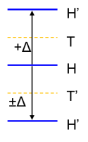
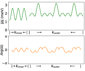
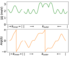
Figure S3: Left: sketch of the vertical interlayer pairing. Middle: Amplitude and winding of the gap function on the Fermi surfaces in the vertical pairing ansatz Eq. (S38) (giving the $E_{\text{1u}}$ irrep), with zero gap winding on the FSs; Right: Amplitude and winding of the gap function on the Fermi surfaces in the vertical pairing ansatz Eq. (S39) (giving the $E_{\text{2u}}$ irrep), with $2\pi$ gap winding on the FSs.

E.4 Comments on the relation between a 2D gap function and a 3D gap function

In the main text, we have been using a 2D Brillouin zone with a 2D gap function $\Delta_{\bm{k},\uparrow}$. The above analysis shows that the gap function $\Delta_{12}(\bm{k},k_{z})$ is intrinsically 3D and is dominant on the $k_{z}=0$ or $k_{z}=\pi$ layers. While a complete calculation of magnetization should involve the full 3D BZ, below we justify the calculation in a 2D BZ layer.

The gap function $\Delta_{12}$ always lives in the odd parity representations. As the character table 2 suggests, the winding of a single Fermi surface is enough to specify whether it lives on the $k_{z}=0$ or the $k_{z}=\pi$ plane in the 3D BZ. For example, if gap winding on the inner and outer Fermi surfaces differ by multiples of $12\pi$, then both lives on the same $k_{z}$ plane in the 3D BZ; otherwise, the gap winding on the inner and outer Fermi surfaces must differ by a multiples of $\pm 3\pi$, $\pm 9\pi$ and so on, and one of the will live in the $k_{z}=0$ plane while the other on the $k_{z}=\pi$ plane. However, as the orbital magnetization receives contributed mainly from the vicinity of the FSs, we can “superpose” the $k_{z}=0$ and $k_{z}=\pi$ planes to get a single 2D BZ, and the calculation of magnetization on this plane should match that of a full 3D calculation. For this reason, we have been using a 2D model in the main text and the sections above, treating the layer indices $\mathrm{H}$ and $\mathrm{H^{\prime}}$ as internal indices. The calculated magnetization should be understood as the result for a full 3D magnetization (i.e. averaged over the momentum planes indexed by $k_{z}$).

As a side comment, when the gap function lives on $k_{z}=\pi$ plane, the $k_{z}=0$ plane remains metallic with a nodal line Fermi surface, yet this nodal line structure may be gapped out by an interlayer tunneling and an intralayer pairing.

Appendix F Further details for the gap equation and free energy

To numerically solve the BCS mean-field equation for the gap function, Eq. (3), we linearize it by substituting the Bogoliubov quasiparticle energy $\varepsilon_{\bm{k}}$ by the normal state quasiparticle energy $E_{\bm{k}}$; near the FSs we further have $E_{\bm{k}}=v_{\bm{k}}k_{\perp}$, where $k_{\perp}=|\bm{k}_{\perp}|$ is the norm of the momentum $\bm{k}_{\perp}$ orthogonal to the Fermi surface tangent, $\bm{k}_{\parallel}$. We also write $d^{2}\bm{k}=dk_{\perp}dk_{\parallel}$. After integrating over $k_{\perp}$ and introducing a cutoff $\Lambda$ (of the order of the Fermi energy), we get

$$\Delta_{\bm{k}}=-V\log\left(\frac{\Lambda}{T_{c}}\right)\int_{\text{FSs}}\frac{dk^{\prime}_{\parallel}}{(2\pi)^{2}v_{\bm{k}^{\prime}}}(\langle u_{\bm{k},\uparrow,\mathrm{H}}|u_{\bm{k}^{\prime},\uparrow,\mathrm{H}}\rangle)^{2}\Delta_{\bm{k}^{\prime}},$$ (S40)

where $T_{c}$ is the transition temperature to be extracted from the solution of Eq. (S40). Clearly, $T_{c}$ depends on the value of the effective attraction $V$; since we cannot estimate $V$ due to lack of enough experimental input, we will not attempt to extract the transition temperature. Our focus will be on the symmetry and topology of the gap function.

Eq. (S40) is then solved as an eigensystem equation. Define

$$M_{\bm{k},\bm{k}^{\prime}}=-\sqrt{\frac{\Delta k\Delta k^{\prime}}{v_{\bm{k}}v_{\bm{k}^{\prime}}}}(\langle u_{\bm{k},\uparrow,\mathrm{H}}|u_{\bm{k}^{\prime},\uparrow,\mathrm{H}}\rangle)^{2},$$ (S41)

which is a symmetric matrix whose rows and columns are labeled by discretized momentum $\bm{k}$ that runs over the two FSs. The largest eigenvalue of $M$ gives the gap solution: denote the corresponding eigenvector as $a_{\bm{k}}$, then the gap function is obtained as

$$\Delta_{\bm{k}}=\sqrt{\frac{v_{\bm{k}}}{\Delta k}}a_{\bm{k}}.$$ (S42)

The amplitude and phase of the solution $\Delta_{\bm{k}}$ is plotted in Fig. 3(b) in the main text.

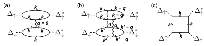
Figure S4: Feynman diagrams at quartic level. The wavy and solid lines represent the propagators for the chiral field $\phi$ and electrons, respectively.

The quartic terms in the Ginzburg-Landau free energy has the form $F_{4}=u(|\Delta_{\uparrow}|^{4}+|\Delta_{\downarrow}|^{4})+v|\Delta_{\uparrow}|^{2}|\Delta_{\downarrow}|^{2}$. Assuming a TRSB field $\phi$ that couples the electrons as an effective Zeeman field, $\phi(n_{\uparrow}-n_{\downarrow})$, where $n_{\sigma}$ is the electron density for spin $\sigma$, the quartic term $v$ is produced by the diagrams in Fig. S4(a)&(b), and the term $u$ by the diagram in Fig. S4(c). However, notice that in Fig. S4(a) the TRSB field propagator carries zero momentum so this diagram gives a vanishing result. The diagram in Fig. S4(b) does not have such a constraint on the TRSB field momentum $\bm{q}$ and it serves as the lowest order diagram contributing to the $v$ term. One concludes that $v\propto\chi^{2}$, where $\chi$ is the susceptibility of the TRSB field $\phi$.

Appendix G Derivation of magnetization formula in a tight binding model

G.1 Normal state

The orbital magnetization is given by Ceresoli et al. (2006)

$$M_{\text{orb}}=\frac{|e|}{\hbar}\sum_{n}\int\frac{d^{2}\bm{k}}{(2\pi)^{2}}\mathrm{Im}\langle\partial_{k_{x}}u_{n\bm{k}}|H_{\bm{k}}+E_{n\bm{k}}-2E_{\text{F}}|\partial_{k_{y}}u_{n\bm{k}}\rangle f_{n\bm{k}}$$ (S43)

In 2D, it has the unit $\frac{e}{\hbar}\text{eV}=e\frac{\text{eV}}{6.582119569\times 10^{-16}\text{eV}\cdot\text{s}}=1.51927\times 10^{15}e\;\text{s}^{-1}=2.52939\frac{\mu_{B}}{V_{\text{2D unit cell}}}$. Therefore,

$$M_{\text{orb}}=\frac{\mu_{B}}{V_{\text{2D unit cell}}}\;2.52939\times\sum_{n}\int\frac{d^{2}\bm{k}}{(2\pi)^{2}}\mathrm{Im}\langle\partial_{k_{x}}u_{n\bm{k}}|\mathsf{H}_{\bm{k}}+\mathsf{E}_{n\bm{k}}-2\mathsf{E}_{\text{F}}|\partial_{k_{y}}u_{n\bm{k}}\rangle f_{n\bm{k}},$$ (S44)

where the sans-serif quantities denote the values when the unit is eV. Note that the orbital magnetization  (S43) contains a localized angular momentum part:

$$M_{\text{orb,atom}} =\frac{-|e|}{2}g_{\text{orb}}\langle\hat{\bm{r}}\times\hat{\bm{v}}\rangle=\frac{-|e|}{2m}g_{\text{orb}}\langle\hat{\bm{r}}\times m\hat{\bm{v}}\rangle=\frac{-|e|\hbar}{2m}g_{\text{orb}}\langle\hat{L}_{z}\rangle=-g_{\text{orb}}\mu_{B}\langle\hat{L}_{z}\rangle$$ (S45)

$$=\frac{\mu_{B}}{V_{\text{2D unit cell}}}\cdot\left(-g_{\text{orb}}\frac{\sqrt{3}}{2}\right)\int\frac{d^{2}\mathsf{k}}{(2\pi)^{2}}\sum_{n}u^{\dagger}_{n\bm{k}}L_{z}u_{n\bm{k}}.$$

A more general derivation for the normal state orbital magnetization leads to Shi et al. (2007)

$$\bm{M}_{\text{orb}}=\frac{1}{\hbar}\sum_{n}\int\frac{d^{2}\bm{k}}{(2\pi)^{2}}\left(f_{n}\bm{m}_{n}+eg_{n}\bm{\Omega}_{n}\right),$$ (S46)

where $f_{n}=f(E_{n\bm{k}})$, $g_{n}=k_{B}T\log(1-f_{n})$, and

$$\bm{m}_{n}=\mathrm{Im}\langle\partial_{\bm{k}_{x}}u_{n\bm{k}}|\times(H_{\bm{k}}-E_{n\bm{k}})|\partial_{\bm{k}_{y}}u_{n\bm{k}}\rangle=\frac{1}{2}\mathrm{Re}\sum_{n^{\prime}\neq n}\mathcal{A}_{nn^{\prime}}\times\bm{J}_{n^{\prime}n},$$ (S47)

where $\mathcal{A}_{nn^{\prime}}$ is the interband Berry connection and $\bm{\Omega}_{n}$ is the single band curvature for band $n$, and $\bm{J}_{n^{\prime}n}=e\bm{v}_{n^{\prime}n}$ is the interband current density, where $\bm{v}_{n^{\prime}n}=\langle u_{n^{\prime}\bm{k}}|\partial_{\bm{k}}H_{\bm{k}}|u_{n\bm{k}}\rangle$ is the interband velocity. It is equivalent to Eq. (S43) with $\bm{M}_{orb}=M_{orb}\hat{\bm{z}}$.

The spin magnetization is

$$M_{\text{spin}}=\frac{1}{2}\mu_{B}g\langle c^{\dagger}c\rangle=\frac{\mu_{B}}{V_{\text{2D unit cell}}}\cdot\frac{\sqrt{3}}{2}\frac{1}{2}g\int\frac{d^{2}\mathsf{k}}{(2\pi)^{2}}f_{n\bm{k}},$$ (S48)

where $\mathsf{k}$ is the numerical value that we use for momentum when the unit is $1/a$.

The total magnetization is the sum of the orbital part and the spin part:

$$M_{\text{total}}=M_{\text{orb}}+M_{\text{spin}}.$$ (S49)

G.2 Superconducting state

We introduce the following notation for the diagonalization of the BdG Hamiltonian: write

$$\mathcal{H}_{\text{BdG}}(\bm{k})=U_{\text{BdG}}(\bm{k})\mathcal{E}(\bm{k})U^{\dagger}_{\text{BdG}}(\bm{k})$$ (S50)

with the energy $\mathcal{E}(\bm{k})=\mathrm{diag}(\varepsilon_{1},\varepsilon_{2},\varepsilon_{3},\varepsilon_{4},\varepsilon_{5},\varepsilon_{6})$. For the unitary matrix $U_{\text{BdG}}(\bm{k})$, we will use the following equivalent notations

$$U_{\text{BdG}}(\bm{k})=\left(\begin{array}[]{cc}[U11]&[U12]\\ {}[U21]&[U22]\end{array}\right).$$ (S51)

We have

$$H_{\text{BdG}}=\sum_{\bm{k}}\left(\sum_{i=1}^{3}\epsilon_{i}\gamma^{\dagger}_{\bm{k}i}\gamma_{\bm{k}i}+\sum_{i=4}^{6}\epsilon_{i}\widetilde{\gamma}^{\dagger}_{\bm{k}i}\widetilde{\gamma}_{\bm{k}i}\right),$$ (S52)

where

$$\left(\begin{array}[]{c}\gamma_{\bm{k}}\\ \widetilde{\gamma}_{\bm{k}}\end{array}\right)=\left(\begin{array}[]{c}\gamma_{\bm{k}}\\ \left(\chi^{\dagger}_{\bm{k}}\right)^{T}\end{array}\right)=U^{\dagger}_{\text{BdG}}\left(\begin{array}[]{c}d_{\bm{k},\uparrow,\mathrm{H}}\\ \left(d^{\dagger}_{-\bm{k},\uparrow,\mathrm{H}^{\prime}}\right)^{T}\end{array}\right).$$ (S53)

We have

$$u_{n\bm{k}}(\bm{r}) =\sum_{\bm{R},\ell}e^{i\bm{k}\cdot(\bm{R}-\bm{r})}u_{\bm{n}\ell}(\bm{k})\phi_{\ell\bm{R}}(\bm{r})=\sum_{\bm{R}}e^{i\bm{k}\cdot(\bm{R}-\bm{r})}w_{n\bm{R}}(\bm{r}),$$ (S54a)

$$w_{n\bm{R}}(\bm{r}) =\sum_{\bm{R}^{\prime}\ell}\phi_{\ell\bm{R}^{\prime}}(\bm{r})\frac{V_{\text{cell}}}{(2\pi)^{3}}\int_{\text{BZ}}e^{i\bm{k}\cdot(\bm{R}^{\prime}-\bm{R})}u_{n\ell}(\bm{k})d^{3}k,$$ (S54b)

$$\bm{r}w_{n\bm{R}}(\bm{r}) =\frac{V_{\text{cell}}}{(2\pi)^{3}}\int_{\text{BZ}}[((-i)\partial_{\bm{k}}+\bm{R})e^{i\bm{k}\cdot(\bm{r}-\bm{R})}]u_{n\bm{k}}(\bm{r})d^{3}k,$$ (S54c)

where $\phi_{\ell\bm{0}}$ is wavefunction for the atomic orbital $\ell$, and $u_{n\ell}(\bm{k})$ is the eigenvector; $u_{n\bm{k}}(\bm{r})$ is the Bloch wavefunction for the $n$th band, and $w_{n\bm{R}}(\bm{r})$ is the wavefunction for the Wannier orbital centered at site $\bm{R}$. Using integrating by parts we also have

$$\bm{r}w_{n\bm{R}}(\bm{r}) =\frac{V_{\text{cell}}}{(2\pi)^{3}}\int_{\text{BZ}}e^{i\bm{k}\cdot(\bm{r}-\bm{R})}(\bm{R}+i\partial_{\bm{k}})u_{n\bm{k}}(\bm{r})d^{3}k$$ (S55)

$$=\frac{V_{\text{cell}}}{(2\pi)^{3}}\int_{\text{BZ}}\sum_{\bm{R}^{\prime},\ell}e^{i\bm{k}\cdot(\bm{R}^{\prime}-\bm{R})}(\bm{R}-\bm{R}^{\prime}+\bm{r}+i\partial_{\bm{k}})u_{n\ell}(\bm{k})\phi_{\ell\bm{R}^{\prime}}(\bm{r})d^{3}k.$$

The full second quantized angular momentum operator is defined as

$$\hat{L}_{z}=\int d\bm{r}\psi^{\dagger}(\bm{r})\hat{l}_{z}\psi(\bm{r}),$$ (S56)

where the quantum field annihilation operator is defined as

$$\psi(\bm{r})=\sum_{\bm{k}}\left(\sum_{i=1}^{3}\langle\bm{r}|\gamma^{\dagger}_{\bm{k}i}|0\rangle\gamma_{\bm{k}i}+\langle\bm{r}|\gamma_{\bm{k}i}|0\rangle\gamma^{\dagger}_{\bm{k}i}+\sum_{i=4}^{6}\langle\bm{r}|\widetilde{\gamma}^{\dagger}_{\bm{k}i}|0\rangle\widetilde{\gamma}_{\bm{k}i}+\langle\bm{r}|\widetilde{\gamma}_{\bm{k}i}|0\rangle\widetilde{\gamma}^{\dagger}_{\bm{k}i}\right),$$ (S57)

In the following, we first derive an expression for $\langle\hat{L}_{z}\rangle$ in terms of the Wannier orbitals, and then convert to tight binding functions. Our derivation parallels that in Ref. Robbins et al. (2020). We have

$$\langle\hat{L}_{z}\rangle =\sum_{\bm{k}}\int d\bm{r}\sum_{i=1}^{3}\langle 0|\gamma_{\bm{k}i}|\bm{r}\rangle\hat{l}_{z}\langle\bm{r}|\gamma_{\bm{k}i}^{\dagger}|0\rangle f_{i}+\langle 0|\gamma^{\dagger}_{\bm{k}i}|\bm{r}\rangle\hat{l}_{z}\langle\bm{r}|\gamma_{\bm{k}i}|0\rangle(1-f_{i})+\sum_{i=4}^{6}\langle 0|\widetilde{\gamma}_{\bm{k}i}|\bm{r}\rangle\hat{l}_{z}\langle\bm{r}|\widetilde{\gamma}_{\bm{k}i}^{\dagger}|0\rangle f_{i}+\langle 0|\widetilde{\gamma}^{\dagger}_{\bm{k}i}|\bm{r}\rangle\hat{l}_{z}\langle\bm{r}|\widetilde{\gamma}_{\bm{k}i}|0\rangle(1-f_{i})$$ (S58)

$$=\sum_{\bm{k}}\int d\bm{r}\sum_{i=1}^{3}\frac{1}{N}\sum_{\bm{R}^{\prime},\bm{R}}e^{i\bm{k}\cdot(-\bm{R}^{\prime}+\bm{R})}\sum_{j^{\prime},j=1}^{3}\phi^{*}_{\bm{R}^{\prime},\uparrow,\mathrm{H},j^{\prime}}(\bm{r})[U11]^{*}_{j^{\prime}i}\hat{l}^{\mathrm{H}}_{z}\phi_{\bm{R},\uparrow,\mathrm{H},j}(\bm{r})[U11]_{ji}f_{i}$$

$$\quad+\sum_{\bm{k}}\int d\bm{r}\sum_{i=1}^{3}\frac{1}{N}\sum_{\bm{R}^{\prime},\bm{R}}e^{i\bm{k}\cdot(\bm{R}^{\prime}-\bm{R})}\sum_{j^{\prime},j=1}^{3}\phi_{\bm{R}^{\prime},\uparrow,\mathrm{H}^{\prime},j^{\prime}}(\bm{r})[U21]_{j^{\prime}i}\hat{l}^{\mathrm{H}^{\prime}}_{z}\phi^{*}_{\bm{R},\uparrow,\mathrm{H^{\prime}},j}(\bm{r})[U21]^{*}_{ji}(1-f_{i})$$

$$\quad+\sum_{\bm{k}}\int d\bm{r}\sum_{i=1}^{3}\frac{1}{N}\sum_{\bm{R}^{\prime},\bm{R}}e^{i\bm{k}\cdot(-\bm{R}^{\prime}+\bm{R})}\sum_{j^{\prime},j=1}^{3}\phi^{*}_{\bm{R}^{\prime},\uparrow,\mathrm{H},j^{\prime}}(\bm{r})[U12]^{*}_{j^{\prime}i}\hat{l}^{\mathrm{H}}_{z}\phi_{\bm{R},\uparrow,\mathrm{H},j}(\bm{r})[U12]_{ji}f_{i+3}$$

$$\quad+\sum_{\bm{k}}\int d\bm{r}\sum_{i=1}^{3}\frac{1}{N}\sum_{\bm{R}^{\prime},\bm{R}}e^{i\bm{k}\cdot(\bm{R}^{\prime}-\bm{R})}\sum_{j^{\prime},j=1}^{3}\phi_{\bm{R}^{\prime},\uparrow,\mathrm{H}^{\prime},j^{\prime}}(\bm{r})[U22]_{j^{\prime}i}\hat{l}^{\mathrm{H}^{\prime}}_{z}\phi^{*}_{\bm{R},\uparrow,\mathrm{H^{\prime}},j}(\bm{r})[U22]^{*}_{ji}(1-f_{i+3})$$

$$=\sum_{\bm{k}}\int d\bm{r}\sum_{i=1}^{3}\frac{1}{N}\sum_{\bm{R}^{\prime},\bm{R}}\left[e^{i\bm{k}\cdot(-\bm{R}^{\prime}+\bm{R})}[W11]^{*}_{i,\bm{R}^{\prime}}(\bm{r})\hat{l}_{z}[W11]_{i,\bm{R}}(\bm{r})f_{i}+e^{i\bm{k}\cdot(\bm{R}^{\prime}-\bm{R})}[W21]_{i,\bm{R}^{\prime}}(\bm{r})\hat{l}_{z}[W21]_{i,\bm{R}}^{*}(\bm{r})(1-f_{i})\right]$$

$$\quad+\sum_{\bm{k}}\int d\bm{r}\sum_{i=1}^{3}\frac{1}{N}\sum_{\bm{R}^{\prime},\bm{R}}\left[e^{i\bm{k}\cdot(-\bm{R}^{\prime}+\bm{R})}[W12]^{*}_{i,\bm{R}^{\prime}}(\bm{r})\hat{l}_{z}[W12]_{i,\bm{R}}(\bm{r})f_{i+3}+e^{i\bm{k}\cdot(\bm{R}^{\prime}-\bm{R})}[W22]_{i,\bm{R}^{\prime}}(\bm{r})\hat{l}_{z}[W22]^{*}_{i,\bm{R}}(\bm{r})(1-f_{i+3})\right]$$

$$=L_{1}+L_{2},$$

where $n_{i}=\sum_{\bm{k}}f_{i,\bm{k}}$ is the density. We used $W$ to denote the Wannier orbitals. $L_{1}$ and $L_{2}$ comes from the decomposition of $\hat{l}_{z}$: by definition $\hat{l}_{z}=\bm{r}\times\bm{v}=\bm{r}\times i\hat{H}(\bm{r})\bm{r}=(\bm{r}-\bm{R})\times i\hat{H}(\bm{r})(\bm{r}-\bm{R})+\bm{R}\times i\hat{H}(\bm{r})(\bm{r}-\bm{R})$, the two terms respectively define $L_{1}$ and $L_{2}$. First, look at the first term: using Eq. (S55) we have $(\bm{r}-\bm{R})[W](\bm{r})=V_{\text{cell}}\int_{\text{BZ}}\frac{d^{3}k}{(2\pi)^{3}}\sum_{\bm{R}^{\prime},\ell}e^{i\bm{k}\cdot(\bm{R}^{\prime}-\bm{R})}(-\bm{R}^{\prime}+\bm{r}+i\partial_{\bm{k}})u_{n\ell}(\bm{k})\phi_{\ell\bm{R}^{\prime}}(\bm{r})$, and

$$L_{1} =i\sum_{\bm{k}}\int d\bm{r}\sum_{i,j^{\prime},j}\frac{1}{N}\sum_{\bm{R}^{\prime},\bm{R},\bm{R}^{\prime}_{1},\bm{R}_{1}}V^{2}_{\text{cell}}\int_{\text{BZ}}\frac{d^{3}k_{1}}{(2\pi)^{3}}e^{-i\bm{k}\cdot\bm{R}^{\prime}}e^{-i\bm{k}^{\prime}_{1}\cdot(\bm{R}^{\prime}_{1}-\bm{R}^{\prime})}(-\bm{R}^{\prime}_{1}+\bm{r}-i\partial_{\bm{k}^{\prime}_{1}})[U11]^{*}_{j^{\prime}i}(\bm{k}^{\prime}_{1})\phi^{*}_{\bm{R}^{\prime}_{1},\uparrow,\mathrm{H},j^{\prime}}(\bm{r})$$ (S59)

$$\qquad\times H_{\mathrm{H}}(\bm{r})\int_{\text{BZ}}\frac{d^{3}k_{1}}{(2\pi)^{3}}e^{i\bm{k}\cdot\bm{R}}e^{i\bm{k}_{1}\cdot(\bm{R}_{1}-\bm{R})}(-\bm{R}_{1}+\bm{r}+i\partial_{\bm{k}_{1}})[U11]_{ji}(\bm{k}_{1})\phi_{\bm{R}_{1},\uparrow,\mathrm{H},j}(\bm{r})f_{i\bm{k}}$$

$$\quad+i\sum_{\bm{k}}\int d\bm{r}\sum_{i,j^{\prime},j^{\prime}}\frac{1}{N}\sum_{\bm{R}^{\prime},\bm{R},\bm{R}^{\prime}_{1},\bm{R}_{1}}V^{2}_{\text{cell}}\int_{\text{BZ}}\frac{d^{3}k^{\prime}_{1}}{(2\pi)^{3}}e^{i\bm{k}\cdot\bm{R}^{\prime}}e^{i\bm{k}^{\prime}_{1}\cdot(\bm{R}^{\prime}_{1}-\bm{R}^{\prime})}(-\bm{R}^{\prime}_{1}+\bm{r}+i\partial_{\bm{k}^{\prime}_{1}})[U21]_{j^{\prime}i}(\bm{k}^{\prime}_{1})\phi^{*}_{\bm{R}^{\prime}_{1},\uparrow,\mathrm{H}^{\prime},j^{\prime}}(\bm{r})$$

$$\qquad\times H_{\mathrm{H}^{\prime}}(\bm{r})\int_{\text{BZ}}\frac{d^{3}k_{1}}{(2\pi)^{3}}e^{-i\bm{k}\cdot\bm{R}}e^{-i\bm{k}_{1}\cdot(\bm{R}_{1}-\bm{R})}(-\bm{R}^{\prime}_{1}+\bm{r}-i\partial_{\bm{k}_{1}})[U21]^{*}_{ji}(\bm{k}_{1})\phi_{\bm{R}_{1},\uparrow,\mathrm{H}^{\prime},j^{\prime}}(\bm{r})(1-f_{i\bm{k}})+...,$$

now the sums over $\bm{R}$ and $\bm{R}^{\prime}$ can be done, which makes $\bm{k}=\bm{k}_{1}=\bm{k}^{\prime}_{1}$. About overall factor: note that $\frac{1}{N}\sum_{\bm{k}}\rightarrow V_{\text{cell}}\int\frac{d^{3}k}{(2\pi)^{3}}$ which can be easily verified. So writing all the integral over $\bm{k}$ as sum, we have $\frac{1}{N^{3}}$. The sum over $\bm{R}$ gives one $N$ factor, and so does the sum over $\bm{R}^{\prime}$, so we are left with $\frac{1}{N}\sum_{\bm{k}}\rightarrow V_{\text{cell}}\int\frac{d^{3}k}{(2\pi)^{3}}$. So we have

$$L_{1} =i\int d\bm{r}\sum_{i,j^{\prime},j}\sum_{\bm{R}^{\prime},\bm{R}}V_{\text{cell}}\int_{\text{BZ}}\frac{d^{3}k}{(2\pi)^{3}}e^{i\bm{k}\cdot(\bm{R}-\bm{R}^{\prime})}(-\bm{R}^{\prime}+\bm{r}-i\partial_{\bm{k}})[U11]^{*}_{j^{\prime}i}(\bm{k})\phi^{*}_{\bm{R}^{\prime},\uparrow,\mathrm{H},j^{\prime}}(\bm{r})\times H_{\mathrm{H}}(\bm{r})(-\bm{R}+\bm{r}+i\partial_{\bm{k}})[U11]_{ji}(\bm{k})\phi_{\bm{R},\uparrow,\mathrm{H},j}(\bm{r})f_{i\bm{k}}$$ (S60)

$$\quad+i\int d\bm{r}\sum_{i,j^{\prime},j}\sum_{\bm{R}^{\prime},\bm{R}}V_{\text{cell}}\int_{\text{BZ}}\frac{d^{3}k}{(2\pi)^{3}}e^{-i\bm{k}\cdot(\bm{R}-\bm{R}^{\prime})}(-\bm{R}^{\prime}+\bm{r}+i\partial_{\bm{k}})[U21]^{*}_{j^{\prime}i}(\bm{k})\phi^{*}_{\bm{R}^{\prime},\uparrow,\mathrm{H}^{\prime},j^{\prime}}(\bm{r})\times H_{\mathrm{H}^{\prime}}(\bm{r})(-\bm{R}+\bm{r}-i\partial_{\bm{k}})[U21]_{ji}(\bm{k})\phi_{\bm{R},\uparrow,\mathrm{H}^{\prime},j}(\bm{r})f_{i\bm{k}}...,$$

then $L_{1}$ is broken into two pieces

$$L_{1} =i\int d\bm{r}\sum_{i,j^{\prime},j}\sum_{\bm{R}^{\prime},\bm{R}}V_{\text{cell}}\int_{\text{BZ}}\frac{d^{3}k}{(2\pi)^{3}}e^{i\bm{k}\cdot(\bm{R}-\bm{R}^{\prime})}(-\bm{R}^{\prime}+\bm{r})[U11]^{*}_{j^{\prime}i}(\bm{k})\phi^{*}_{\bm{R}^{\prime},\uparrow,\mathrm{H},j^{\prime}}(\bm{r})\times H_{\mathrm{H}}(\bm{r})(-\bm{R}+\bm{r})[U11]_{ji}(\bm{k})\phi_{\bm{R},\uparrow,\mathrm{H},j}(\bm{r})f_{i\bm{k}}$$ (S61)

$$\quad+i\int d\bm{r}\sum_{i,j^{\prime},j}\sum_{\bm{R}^{\prime},\bm{R}}e^{i\bm{k}\cdot(\bm{R}-\bm{R}^{\prime})}V_{\text{cell}}\int_{\text{BZ}}\frac{d^{3}k}{(2\pi)^{3}}\partial_{\bm{k}}[U11]^{*}_{j^{\prime}i}(\bm{k})\phi^{*}_{\bm{R}^{\prime},\uparrow,\mathrm{H},j^{\prime}}(\bm{r})\times H_{\mathrm{H}}(\bm{r})\partial_{\bm{k}}[U11]_{ji}(\bm{k})\phi_{\bm{R},\uparrow,\mathrm{H},j}(\bm{r})f_{i\bm{k}}$$

$$\quad+i\int d\bm{r}\sum_{i,j^{\prime},j}\sum_{\bm{R}^{\prime},\bm{R}}V_{\text{cell}}\int_{\text{BZ}}\frac{d^{3}k}{(2\pi)^{3}}e^{i\bm{k}\cdot(\bm{R}^{\prime}-\bm{R})}(-\bm{R}^{\prime}+\bm{r})[U21]_{j^{\prime}i}(\bm{k})\phi_{\bm{R}^{\prime},\uparrow,\mathrm{H}^{\prime},j^{\prime}}(\bm{r})\times H_{\mathrm{H}^{\prime}}(\bm{r})(-\bm{R}+\bm{r})[U21]^{*}_{ji}(\bm{k})\phi^{*}_{\bm{R},\uparrow,\mathrm{H}^{\prime},j}(\bm{r})(1-f_{i\bm{k}})$$

$$\quad+i\int d\bm{r}\sum_{i,j^{\prime},j}\sum_{\bm{R}^{\prime},\bm{R}}e^{i\bm{k}\cdot(\bm{R}^{\prime}-\bm{R})}V_{\text{cell}}\int_{\text{BZ}}\frac{d^{3}k}{(2\pi)^{3}}\partial_{\bm{k}}[U21]_{j^{\prime}i}(\bm{k})\phi_{\bm{R}^{\prime},\uparrow,\mathrm{H}^{\prime},j^{\prime}}(\bm{r})\times H_{\mathrm{H}^{\prime}}(\bm{r})\partial_{\bm{k}}[U21]^{*}_{ji}(\bm{k})\phi^{*}_{\bm{R},\uparrow,\mathrm{H}^{\prime},j}(\bm{r})(1-f_{i\bm{k}})$$

$$\quad+...,$$

the first (and the third…) line gives the atomic angular momentum (and this sets $\bm{R}-\bm{R}^{\prime}$) while the second (and the fourth…) line gives the Bloch angular momentum. Carrying out the integral over $\bm{r}$ gives:

$$\sum_{\bm{R}^{\prime},\bm{R}}e^{i\bm{k}\cdot(\bm{R}-\bm{R}^{\prime})}\int d\bm{r}\phi^{*}_{\bm{R}^{\prime},\uparrow,\mathrm{H},j^{\prime}}(\bm{r})\times H_{\mathrm{H}}(\bm{r})\phi_{\bm{R},\uparrow,\mathrm{H},j}(\bm{r})=\sum_{\bm{R}^{\prime},\bm{R}}\int e^{i\bm{k}\cdot(\bm{R}-\bm{R}^{\prime})}[H_{\mathrm{H},\bm{R}^{\prime},\bm{R}}]_{j^{\prime},j}=H_{\mathrm{H}}(\bm{k})_{j^{\prime},j},$$

$$\sum_{\bm{R}^{\prime},\bm{R}}e^{i\bm{k}\cdot(\bm{R}^{\prime}-\bm{R})}\int d\bm{r}\phi_{\bm{R}^{\prime},\uparrow,\mathrm{H},j^{\prime}}(\bm{r})\times H_{\mathrm{H}^{\prime}}(\bm{r})\phi^{*}_{\bm{R},\uparrow,\mathrm{H},j}(\bm{r})=\sum_{\bm{R}^{\prime},\bm{R}}\int e^{i\bm{k}\cdot(\bm{R}^{\prime}-\bm{R})}[H_{\mathrm{H^{\prime}},\bm{R}^{\prime},\bm{R}}]_{j^{\prime},j}=H_{\mathrm{H^{\prime}}}(-\bm{k})_{j^{\prime},j},$$

where we have used the fact that all the $\phi_{j}$ are real (they are $d_{xy}$, $d_{x^{2}-y^{2}}$ and $d_{z^{2}}$ orbitals). Therefore, we have

$$L_{1} =\sum_{i,j^{\prime},j}V_{\text{cell}}\int_{\text{BZ}}\frac{d^{3}k}{(2\pi)^{3}}\left\{[U11]^{*}_{j^{\prime}i}(\bm{k})l^{\mathrm{H}}_{j^{\prime}j}[U11]_{ji}(\bm{k})+i\partial_{\bm{k}}[U11]^{*}_{j^{\prime}i}(\bm{k})\times H_{\mathrm{H}}(\bm{k})_{j^{\prime}j}\partial_{\bm{k}}[U11]_{{}^{\prime}i}(\bm{k})\right\}f_{i\bm{k}}$$ (S62)

$$\quad+\sum_{i,j^{\prime},j}V_{\text{cell}}\int_{\text{BZ}}\frac{d^{3}k}{(2\pi)^{3}}\left\{[U21]_{j^{\prime}i}(\bm{k})l^{\mathrm{H}^{\prime}}_{j^{\prime}j}[U21]^{*}_{ji}(\bm{k})+i\partial_{\bm{k}}[U21]_{j^{\prime}i}(\bm{k})\times H_{\mathrm{H}^{\prime}}(-\bm{k})_{j^{\prime}j}\partial_{\bm{k}}[U21]^{*}_{ji}(\bm{k})\right\}(1-f_{i\bm{k}})$$

$$\quad+...$$

$$=\sum_{i,j^{\prime},j}V_{\text{cell}}\int_{\text{BZ}}\frac{d^{3}k}{(2\pi)^{3}}\left\{[U11]^{*}_{j^{\prime}i}(\bm{k})l_{j^{\prime}j}[U11]_{ji}(\bm{k})+i\partial_{\bm{k}}[U11]^{*}_{j^{\prime}i}(\bm{k})\times H_{\mathrm{H}}(\bm{k})_{j^{\prime}j}\partial_{\bm{k}}[U11]_{{}^{\prime}i}(\bm{k})\right\}f_{i\bm{k}}$$

$$\quad+\sum_{i,j^{\prime},j}V_{\text{cell}}\int_{\text{BZ}}\frac{d^{3}k}{(2\pi)^{3}}\left\{-[U21]^{*}_{j^{\prime}i}(\bm{k})l_{j^{\prime}j}[U21]_{ji}(\bm{k})-i\partial_{\bm{k}}[U21]^{*}_{j^{\prime}i}(\bm{k})\times H^{T}_{\mathrm{H}}(\bm{k})_{j^{\prime}j}\partial_{\bm{k}}[U21]_{ji}(\bm{k})\right\}(1-f_{i\bm{k}})$$

$$\quad+\sum_{i,j^{\prime},j}V_{\text{cell}}\int_{\text{BZ}}\frac{d^{3}k}{(2\pi)^{3}}\left\{[U12]^{*}_{j^{\prime}i}(\bm{k})l_{j^{\prime}j}[U12]_{ji}(\bm{k})+i\partial_{\bm{k}}[U12]^{*}_{j^{\prime}i}(\bm{k})\times H_{\mathrm{H}}(\bm{k})_{j^{\prime}j}\partial_{\bm{k}}[U12]_{ji}(\bm{k})\right\}f_{i+3,\bm{k}}$$

$$\quad+\sum_{i,j^{\prime},j}V_{\text{cell}}\int_{\text{BZ}}\frac{d^{3}k}{(2\pi)^{3}}\left\{-[U22]^{*}_{j^{\prime}i}(\bm{k})l_{j^{\prime}j}[U22]_{ji}(\bm{k})-i\partial_{\bm{k}}[U22]^{*}_{j^{\prime}i}(\bm{k})\times H^{T}_{\mathrm{H}}(\bm{k})_{j^{\prime}j}\partial_{\bm{k}}[U22]_{ji}(\bm{k})\right\}(1-f_{i+3,\bm{k}})$$

We write the above as

$$L_{1}=V_{\text{cell}}\int\frac{d^{3}k}{(2\pi)^{3}}U^{\dagger}_{\text{BdG}}\left(1_{2\times 2}\otimes l\right)U_{\text{BdG}}+i\partial_{\bm{k}}U^{\dagger}_{\text{BdG}}\left(\begin{array}[]{cc}\mathcal{H}_{\mathrm{H}}(\bm{k})&\\ &-\mathcal{H}^{T}_{\mathrm{H}}(\bm{k})\end{array}\right)\left(\begin{array}[]{ll}\partial_{\bm{k}}[U11](\bm{k})f_{1:3,\bm{k}}&\partial_{\bm{k}}[U12](\bm{k})f_{4:6,\bm{k}}\\ \partial_{\bm{k}}[U21](\bm{k})(1-f_{1:3,\bm{k}})&\partial_{\bm{k}}[U22](\bm{k})(1-f_{4:6},\bm{k})\end{array}\right),$$ (S63)

where $l$ is the $3\times 3$ matrix in the orbital basis, and $U_{\text{BdG}}=U_{\text{BdG}}(\bm{k})$. Then, note that magnetization is proportional to charge times angular momentum, so we define $M_{\text{LC}}=\frac{-eL_{1}}{V_{\text{cell}}}$ (note $e=|e|$ is the absolute value of the charge) and

$$M_{\text{LC}}=-e\;\mathrm{ReTr}\int_{\text{BZ}}\frac{d^{2}k}{(2\pi)^{2}}U^{\dagger}_{\text{BdG}}\left(1_{2\times 2}\otimes l\right)U_{\text{BdG}}+e\;\mathrm{ImTr}\int_{\text{BZ}}\frac{d^{2}k}{(2\pi)^{2}}\partial_{\bm{k}}U^{\dagger}_{\text{BdG}}\times\left(\mathcal{H}_{\text{BdG}}\Big{|}_{\Delta=0}\right)\left(\begin{array}[]{l}\partial_{\bm{k}}[U_{\text{BdG}}]_{1:3,:}f_{:,\bm{k}}\\ \partial_{\bm{k}}[U_{\text{BdG}}]_{4:6,:}(1-f_{:,\bm{k}})\end{array}\right).$$ (S64)

The overall signs matches through in Eq. (10) and (11) of Ref. Robbins et al. (2020) (note that in Robbins et al. (2020) $\gamma\propto-e$ carries a sign).

One can verify that when pairing term is zero the above formula correctly reduces to the normal state magnetization

Then we have the second term $L_{2}$, that contains $\bm{R}\times i\hat{H}(\bm{r})(\bm{r}-\bm{R})$. In parallel with Robbins et al. (2020), we propose that this term has the expression

$$M_{\text{IC}}=e\int\frac{d^{3}k}{(2\pi)^{3}}\mathrm{Im}\left\{\partial_{\bm{k}}U^{\dagger}_{\text{BdG}}\times\mathcal{E}_{:}\left(\begin{array}[]{l}\partial_{\bm{k}}[U_{\text{BdG}}]_{1:3,:}f_{:,\bm{k}}\\ \partial_{\bm{k}}[U_{\text{BdG}}]_{4:6,:}(1-f_{:,\bm{k}})\end{array}\right)\right\},$$ (S65)

where $\mathcal{E}_{:}=\mathcal{E}=\mathrm{diag}(\varepsilon_{1},...,\varepsilon_{6}).$ This term corresponds to the second term in the normal state orbital magnetization, Eq. (S46), and is related to the Berry curvature of the BdG bands.

To summarize, the bulk magnetization consists of three parts:

$$M^{z}=M^{z}_{\text{orb,t-b}}+M^{z}_{\text{orb,atom}}+M^{z}_{\text{spin}},$$ (S66)

where the last two terms are the atomic angular momentum and atomic spin contribution to the magnetization, which can be unambiguously written as

$$M^{z}_{\text{orb,atom}} =-\frac{\mu_{B}}{V_{\text{2D unit cell}}}\cdot\frac{\sqrt{3}}{2}\mathrm{ReTr}\int_{\text{BZ}}\frac{d^{2}k}{(2\pi)^{2}}U^{\dagger}_{\text{BdG}}\left(\begin{array}[]{cc}L^{z}&0\\ 0&-L^{z}\end{array}\right)\left(\begin{array}[]{l}{[U_{\text{BdG}}]}_{1:3}f_{\bm{k}}\\ {[U_{\text{BdG}}]}_{4:6}(1-f_{\bm{k}})\end{array}\right),$$ (S67e)

$$M^{z}_{\text{spin}} =\frac{g_{s}}{2}\frac{\mu_{B}}{V_{\text{2D unit cell}}}\cdot\frac{\sqrt{3}}{2}\mathrm{ReTr}\int_{\text{BZ}}\frac{d^{2}k}{(2\pi)^{2}}U^{\dagger}_{\text{BdG}}\left(\begin{array}[]{l}{[U_{\text{BdG}}]}_{1:3}f_{\bm{k}}\\ {[U_{\text{BdG}}]}_{4:6}(1-f_{\bm{k}})\end{array}\right),$$ (S67h)

where $g_{s}\approx 2$ is the spin $g$-factor, $U_{\text{BdG}}$ is the matrix of eigenvectors: $\mathcal{H}_{\text{BdG}}(\bm{k})=U_{\text{BdG}}(\bm{k})\mathcal{E}_{\bm{k}}U^{\dagger}_{\text{BdG}}(\bm{k})$, $f_{\bm{k}}=f(\mathcal{E}_{\bm{k}})$ is a diagonal matrix, and $[U_{\text{BdG}}]_{1:3}$ denotes the first three rows of $U_{\text{BdG}}$. $M^{z}_{\text{orb,atom}}$ and $M^{z}_{\text{spin}}$ can be computed numerically without difficulty.

The first term in Eq. (S66), $M^{z}_{\text{orb,t-b}}$, denotes the orbital magnetization due to hopping and pairing, and has the form

$$M^{z}_{\text{orb,t-b}}= M_{\text{IC}}+M_{\text{LC}}$$ (S68)

$$= \frac{\mu_{B}}{V_{\text{2D unit cell}}}\;2.52939\times\mathrm{ImTr}\int\frac{d^{3}k}{(2\pi)^{3}}\partial_{\bm{k}}U^{\dagger}_{\text{BdG}}\times\mathcal{E}_{:}\left(\begin{array}[]{l}\partial_{\bm{k}}[U_{\text{BdG}}]_{1:3,:}f_{:,\bm{k}}\\ \partial_{\bm{k}}[U_{\text{BdG}}]_{4:6,:}(1-f_{:,\bm{k}})\end{array}\right)$$

$$+\frac{\mu_{B}}{V_{\text{2D unit cell}}}\;2.52939\times\;\mathrm{ImTr}\int_{\text{BZ}}\frac{d^{2}k}{(2\pi)^{2}}\partial_{\bm{k}}U^{\dagger}_{\text{BdG}}\times\left(\mathcal{H}_{\text{BdG}}\Big{|}_{\Delta=0}\right)\left(\begin{array}[]{l}\partial_{\bm{k}}[U_{\text{BdG}}]_{1:3,:}f_{:,\bm{k}}\\ \partial_{\bm{k}}[U_{\text{BdG}}]_{4:6,:}(1-f_{:,\bm{k}})\end{array}\right).$$

Note that we used the unit $\mu_{B}/V_{\text{u.c.}}$ in the main text for magnetization, which is related to the magnetization per a single $\mathrm{H}$ (or $\mathrm{H^{\prime}}$) layer (with unit of $\mu_{B}/V_{\text{2D unit cell}}$) by a factor of 2.

Appendix H Numerical results

H.1 Normal state magnetization

First, the normal state magnetization in the spin up sector is

$$(M^{z}_{\text{orb,t-b},\uparrow},M^{z}_{\text{orb,atom},\uparrow},M^{z}_{\text{spin},\uparrow})=(-0.0840,0.246,0.944)\;\mu_{\text{B}}/V_{\text{u.c.}}.$$ (S69)

Then, we calculate the total magnetization $M_{\uparrow}+M_{\downarrow}$ in presence of a magnetic field $B$. When $B=0$ we have $M_{\uparrow}+M_{\downarrow}=0$. When $B=5$ T, we have

$$(M^{z}_{\text{orb,t-b},\uparrow+\downarrow},M^{z}_{\text{orb,atom},\uparrow+\downarrow},M^{z}_{\text{spin},\uparrow+\downarrow})=(-0.000280,-0.000416,0.00182)\;\mu_{\text{B}}/V_{\text{u.c.}}.$$ (S70)

Table 3: Magnetization for the three ansatze at temperatures $T=1$ K, 2 K, 5 K at gap size of $0.44$ meV and zero magnetic field. The magnetization is in the units of $10^{-4}\,\mu_{B}/V_{\text{u.c.}}$, where $V_{\text{u.c.}}$ is the volume of the four-layer unit cell of 4Hb-TaS₂.

Ansatze	$c_{\text{BdG}}=+3$			$c_{\text{BdG}}=0$			$c_{\text{BdG}}=-3$
Magnetization	${M_{\text{orb,t-b},\uparrow+\downarrow}}$	$M_{\text{orb,atom},\uparrow+\downarrow}$	$M_{\text{spin},\uparrow+\downarrow}$	${M_{\text{orb,t-b},\uparrow+\downarrow}}$	$M_{\text{orb,atom},\uparrow+\downarrow}$	$M_{\text{spin},\uparrow+\downarrow}$	${M_{\text{orb,t-b},\uparrow+\downarrow}}$	$M_{\text{orb,atom},\uparrow+\downarrow}$	$M_{\text{spin},\uparrow+\downarrow}$
$T=1$ K	$4.56$	$-1.52$	$3.04$	$-1.64$	$-5.48$	$6.92$	$-10.0$	$-0.604$	$2.18$
$T=2$ K	$3.58$	$-1.50$	$2.82$	$-2.58$	$-5.44$	$6.70$	$-10.9$	$-1.46$	$1.96$
$T=5$ K	$2.70$	$-1.56$	$2.22$	$-3.16$	$-5.52$	$5.94$	$-11.2$	$-0.238$	$10.1$

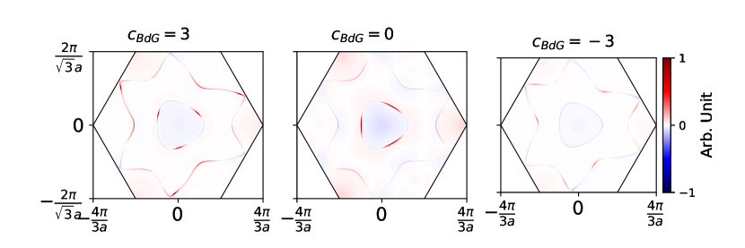
Figure S5: Berry curvature for the three Ansatze with $c_{\text{BdG}}=+3,0,-3$.

H.2 Superconducting state magnetization: further plots

We compute the total magnetization $M$ as a function of the gap size $\Delta$ using Eq. (S66). The result is shown in Fig. (S6), for temperatures $T=1$ K ,2 K, and 5 K.

For the realistic gap size $\Delta=0.44$ meV, we also compute the components of the magnetization, ${M_{\text{orb,t-b},\uparrow+\downarrow}}$, $M_{\text{orb,atom},\uparrow+\downarrow}$, $M_{\text{spin},\uparrow+\downarrow}$, at three temperatures $T=1$ K ,2 K, and 5 K. The result is given in Table 3.

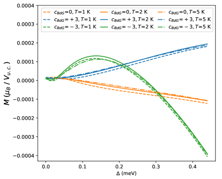
Figure S6: Total magnetization $M$ as a function of the gap size $\Delta$ for the three ansatze with $c_{\text{BdG}}=+3,0,-3$ at zero field for three temperatures $T=1$ K, 2 K, 5 K.

The magnetization as a function of $E_{\uparrow}-E_{\downarrow}$ induced by the TRSB order parameter $\phi$ for the two vertical pairing states Eq. (S38) and Eq. (S39) is shown in Fig. S7.

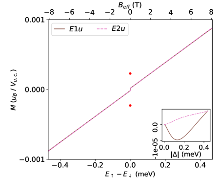
Figure S7: Magnetization in the vertical pairing interlayer pairing ansatze (S38) and (S39) with a gap size of 0.44 meV. The lower and upper horizontal axes are related by $E_{\uparrow}-E_{\downarrow}=\mu_{\text{B}}B_{\text{eff}}$.The two red dots denote the remnant magnetization inferred from the experiment Persky et al. (2022). The inset shows the magnetization as a function of the gap size for the three pairing ansatze. Magnetizations are calculated at $T=2$ K.

References

• Persky et al. (2022) E. Persky, A. V. Bjørlig, I. Feldman, A. Almoalem, E. Altman, E. Berg, I. Kimchi, J. Ruhman, A. Kanigel,  and B. Kalisky, Nature 607, 692 (2022).
• Wilson et al. (1975) J. A. Wilson, F. Di Salvo,  and S. Mahajan, Advances in Physics 24, 117 (1975).
• Kim et al. (1994) J.-J. Kim, W. Yamaguchi, T. Hasegawa,  and K. Kitazawa, Phys. Rev. Lett. 73, 2103 (1994).
• Perfetti et al. (2006) L. Perfetti, P. Loukakos, M. Lisowski, U. Bovensiepen, H. Berger, S. Biermann, P. Cornaglia, A. Georges,  and M. Wolf, Physical review letters 97, 067402 (2006).
• Wang et al. (2018) Z. Wang, Y.-Y. Sun, I. Abdelwahab, L. Cao, W. Yu, H. Ju, J. Zhu, W. Fu, L. Chu, H. Xu, et al., ACS nano 12, 12619 (2018).
• Gao et al. (2020) J. J. Gao, J. G. Si, X. Luo, J. Yan, Z. Z. Jiang, W. Wang, Y. Y. Han, P. Tong, W. H. Song, X. B. Zhu, Q. J. Li, W. J. Lu,  and Y. P. Sun, Phys. Rev. B 102, 075138 (2020).
• Nayak et al. (2021) A. K. Nayak, A. Steinbok, Y. Roet, J. Koo, G. Margalit, I. Feldman, A. Almoalem, A. Kanigel, G. A. Fiete, B. Yan, et al., Nature physics 17, 1413 (2021).
• Nayak et al. (2023) A. K. Nayak, A. Steinbok, Y. Roet, J. Koo, I. Feldman, A. Almoalem, A. Kanigel, B. Yan, A. Rosch, N. Avraham, et al., arXiv preprint arXiv:2303.01447  (2023).
• Ribak et al. (2020) A. Ribak, R. M. Skiff, M. Mograbi, P. K. Rout, M. H. Fischer, J. Ruhman, K. Chashka, Y. Dagan,  and A. Kanigel, Science Advances 6, eaax9480 (2020)https://www.science.org/doi/pdf/10.1126/sciadv.aax9480 .
• Liu et al. (2013) G.-B. Liu, W.-Y. Shan, Y. Yao, W. Yao,  and D. Xiao, Physical Review B 88, 085433 (2013).
• (11) See Supplemental Material for a discussion of pairing mechanism and phase diagram, the details of lattice symmetry, the tight-binding model for the normal state, the BdG Hamiltonian of the three pairing ansatze, symmetry and topology of the gap function, comments on a 2D treatment of the 3D gap function, the derivation and numerical simulation of the gap equation and magnetization formulas.
• Margalit et al. (2021) G. Margalit, E. Berg,  and Y. Oreg, Annals of Physics 435, 168561 (2021), special issue on Philip W. Anderson.
• (13) SQUID sensitivity taken from https://beenalab.biu.ac.il/.
• (14) It is worth noting that there may be an anomalously wide separation between the two transition temperatures even at the quadratic level because the bands are close to a Van Hove singularity. In a weakly ferromagnetic state the majority component gets closer to it, while the minority gets further, which can lead to a sizable difference even for small magnetization.
• Shi et al. (2007) J. Shi, G. Vignale, D. Xiao,  and Q. Niu, Phys. Rev. Lett. 99, 197202 (2007).
• (16) We refer to Supplemental Material Not for two vertical bond pairing ansatze having gap functions in the irreps $E_{u}$ and their magnetization.
• Dentelski et al. (2021) D. Dentelski, E. Day-Roberts, T. Birol, R. M. Fernandes,  and J. Ruhman, Phys. Rev. B 103, 224522 (2021).
• König (2023) E. J. König, arXiv e-prints , arXiv:2306.07871 (2023)arXiv:2306.07871 [cond-mat.str-el] .
• Wang et al. (2021) D. Wang, J. Wiebe, R. Zhong, G. Gu,  and R. Wiesendanger, Phys. Rev. Lett. 126, 076802 (2021).
• Fischer et al. (2022) M. H. Fischer, M. Sigrist, D. F. Agterberg,  and Y. Yanase, arXiv preprint arXiv:2204.02449  (2022).
• Möckli and Khodas (2018) D. Möckli and M. Khodas, Phys. Rev. B 98, 144518 (2018).
• Ceresoli et al. (2006) D. Ceresoli, T. Thonhauser, D. Vanderbilt,  and R. Resta, Phys. Rev. B 74, 024408 (2006).
• Robbins et al. (2020) J. Robbins, J. F. Annett,  and M. Gradhand, Phys. Rev. B 101, 134505 (2020).