Convergence Guarantees for Stochastic Subgradient Methods in Nonsmooth Nonconvex Optimization

Abstract

In this paper, we investigate the convergence properties of the stochastic gradient descent (SGD) method and its variants, especially in training neural networks built from nonsmooth activation functions. We develop a novel framework that assigns different timescales to stepsizes for updating the momentum terms and variables, respectively. Under mild conditions, we prove the global convergence of our proposed framework in both single-timescale and two-timescale cases. We show that our proposed framework encompasses a wide range of well-known SGD-type methods, including heavy-ball SGD, SignSGD, Lion, normalized SGD and clipped SGD. Furthermore, when the objective function adopts a finite-sum formulation, we prove the convergence properties for these SGD-type methods based on our proposed framework. In particular, we prove that these SGD-type methods find the Clarke stationary points of the objective function with randomly chosen stepsizes and initial points under mild assumptions. Preliminary numerical experiments demonstrate the high efficiency of our analyzed SGD-type methods.

1 Introduction

In this paper, we consider the following unconstrained optimization problem,

$$\min_{x\in\mathbb{R}^{n}}\quad f(x).$$ (UOP)

Here the objective function $f:\mathbb{R}^{n}\to\mathbb{R}$ is assumed to be nonconvex and locally Lipschitz continuous over $\mathbb{R}^{n}$. The optimization problem UOP encompasses a great number of tasks related to training neural networks, especially when these neural networks employ the rectified linear unit (ReLU) and leaky ReLU [26] as activation functions.

Over the past several decades, a great number of optimization approaches have been developed for solving UOP. Among these methods, the stochastic gradient descent (SGD) method [30] is one of the most popular optimization methods. Then based on the SGD method, a great number of SGD-type methods are proposed. For instance, the heavy-ball SGD method [29] introduces heavy-ball momentum terms into the iteration process to enhance performance. Moreover, the signSGD method [5] updates along the sign of a stochastic gradient as a means of normalization, leading to reduced memory consumption while promoting efficient communications in distributed settings. In addition, the normalized SGD [38, 39, 17] is proposed by normalizing the updating direction in SGD to the unit sphere, while demonstrating remarkable efficiency in training large language models [38, 39]. Furthermore, the clipped SGD method [41, 40] is developed by employing the clipping operator to avoid extreme values in the update direction, hence accelerating the training under heavy-tailed noises. Recently, [14] proposes a new variant of the SGD method named the second-order inertial optimization method (INNA), which is derived from the ordinary differential equations proposed in [2, 1]. Very recently, inspired by the techniques for automatically discovering optimization algorithms [3, 27], the authors in [15] formulate the algorithm discovery as a program search problem and conduct policy search within several predefined mathematical function pools. Their proposed method discovers a simple and effective variant of the SGD method named the evolved sign momentum (Lion). As discussed in [42], these SGD-type methods exhibit low memory consumption and excellent generalization performance, making them popular in various training scenarios, such as diffusion models [15], knowledge distillation [37], meta-learning [23], and large language models [38, 39], etc.

Despite recent progress in developing highly efficient methods based on the SGD framework, the convergence analysis for these SGD-type methods remains limited. As illustrated in [11], nonsmooth activation functions, including ReLU and leaky ReLU, are commonly employed in neural network architectures. Consequently, the loss functions of these neural networks are usually nonsmooth and lack Clarke regularity (e.g., differentiability, weak convexity, etc.). However, most of the existing works only focus on cases where $f$ is differentiable or weakly convex, thus precluding various important applications in training nonsmooth neural networks.

Towards the nonsmoothness of the neural networks, some recent works [18, 31, 7, 11, 14, 12, 25] employ the concept of differential inclusion to establish the convergence properties for the SGD method in training nonsmooth neural networks. In particular, [31] analyzed the heavy-ball proximal SGD method with single-timescale stepsizes for minimizing Norkin subdifferentiable functions [28]. That class of functions belongs to the class of potential functions [11, Definition 3], according to [31, Theorem 1] and [11, Corollary 2]. Very recently, [25] investigated the convergence to essential accumulation points [12] for heavy-ball SGD methods in the minimization of potential functions, based on the closed-measure approach proposed by [7]. Furthermore, [22, 23] apply these methods to solving manifold optimization problems using the constraint dissolving approach [36]. In addition, [32, 20] design stochastic subgradient methods for solving multi-level composition optimization problems.

However, these works are limited to the SGD method and heavy-ball SGD method, rendering them inapplicable to some recently proposed SGD variants, such as Lion, signSGD, and normalized SGD. Moreover, the SGD-type methods analyzed in [18, 31, 7, 11, 14, 22, 25] assume single-timescale stepsizes, where the decay rate of the stepsize for updating the momentum terms matches that of the stepsize for updating the variables. In practical implementations of SGD-type methods, stepsizes often follow a two-timescale scheme, where the stepsize for updating the momentum terms decays at a much slower rate than the stepsize for updating the variables. To the best of our knowledge, no existing work has established the convergence properties for SGD methods with two-timescale stepsizes.

As the number of emerging variants of the SGD method continues to increase, and our limited understanding of their convergence properties for training nonsmooth neural networks persists, we are motivated to ask the following question:

Can we develop a unified framework to establish the convergence properties for these SGD-type methods under realistic settings, especially in training nonsmooth neural networks with possibly two-timescale stepsizes?

In the process of training neural networks, a key challenge arises from how to differentiate their loss functions. Automatic differentiation (AD) algorithms serve as an essential tool for computing the differential of the loss function in neural networks and have become the default choice in numerous deep learning packages, such as TensorFlow, PyTorch, and JAX. When employed for differentiating a neural network, AD algorithms yield the differential of the loss function by recursively composing the Jacobians of each block of the neural network based on the chain rule. However, when applied to nonsmooth neural networks, the outputs of AD algorithms are usually not in the Clarke subdifferential of the network [10], since the chain rule fails for general nonsmooth functions [16]. To address this issue, [11] introduced the concept of a conservative field, which is a generalization of the Clarke subdifferential. In their work, they showed that for any given definable loss function $f$, there exists a set-valued mapping $\mathcal{D}_{f}:\mathbb{R}^{n}\rightrightarrows\mathbb{R}^{n}$, referred to as the conservative field, which can serve as a surrogate of the Clarke subdifferential. [11] shows that for any $x\in\mathbb{R}^{n}$, the outputs of AD algorithms are always contained within $\mathcal{D}_{f}(x)$. Therefore, the concept of the conservative field provides a way to interpret how AD algorithms work in differentiating nonsmooth neural networks.

Contributions

In this paper, we employ the concept of the conservative field to characterize how we differentiate the neural network. The main contributions of our paper are summarized as follows:

• A general framework for SGD-type methods
  We propose a set-valued mapping that provides a generalized characterization of the update schemes for a class of SGD-type methods,

  $$\mathcal{G}(x,m)=\left\{\left[\begin{matrix}\mathcal{D}_{\phi}(m)+\alpha d\\ m-d\\ \end{matrix}\right]:d\in\mathcal{D}_{f}(x)\right\}.$$ (1.1)

  Here $\mathcal{D}_{f}$ is the conservative field for $f$ that describes how $f$ is differentiated, while $\mathcal{D}_{\phi}$ is a conservative field for an auxiliary function $\phi$ that characterizes the updating scheme of ${x_{k}}$. Moreover, we introduce a hyper-parameter $\alpha\geq 0$ for the Nesterov momentum term. With the set-valued mapping $\mathcal{G}$, we consider the following framework that generalizes the updating schemes for a wide variety of SGD-type methods,

  $$\left\{\begin{aligned} {x_{k+1}}={}&{x_{k}}-\eta_{k}(d_{x,k}+\xi_{x,k}),\\ {m_{k+1}}={}&{m_{k}}-\theta_{k}(d_{m,k}+\xi_{m,k}).\\ \end{aligned}\right.$$ (GSGD)

  Here $(d_{x,k},d_{m,k})$ is an approximated evaluation of the elements in $\mathcal{G}({x_{k}},{m_{k}})$, while $(\xi_{x,k},\xi_{m,k})$ corresponds to the noise in evaluating $(d_{x,k},d_{m,k})$. Moreover, $\{\eta_{k}\}$ and $\{\theta_{k}\}$ are two positive sequences of stepsizes for updating the variables $\{{x_{k}}\}$ and momentum terms $\{{m_{k}}\}$, respectively.

• Convergence properties with single-timescale and two-timescale stepsizes
  Under both cases where the stepsizes in framework (GSGD) are chosen as single-timescale (i.e., $\theta_{k}/\eta_{k}\to\tau$ for some constant $\tau>0$) or two-timescale (i.e., $\theta_{k}/\eta_{k}\to+\infty$), we show that their iterates are asymptotically equivalent to the trajectories of a particular differential inclusion (see Section 2.3 for details). Then under mild conditions that are applicable to most deep learning problems, we prove that almost surely, any cluster point of the sequence $\{{x_{k}}\}$ generated by our proposed framework (GSGD) is a $\mathcal{D}_{f}$-stationary point of $f$. Notably, our theoretical analysis only requires the stepsizes $\{\eta_{k}\}$ and $\{\theta_{k}\}$ to diminish at a rate of $o(1/\log(k))$, hence providing great flexibility in the selection of these stepsizes in practical implementations.

• Guaranteed convergence for SGD-type methods in deep learning
  We demonstrate that our proposed framework can be employed to analyze the convergence properties for a class of SGD-type methods, including heavy-ball SGD, Lion, signSGD, and normalized SGD. Specifically, when the objective function $f$ takes a finite-sum formulation, we show that these SGD-type methods converge to stationary points of $f$ in both senses of conservative field and Clarke subdifferential under mild conditions.

  Preliminary numerical experiments illustrate that for both the single-timescale and two-timescale stepsizes cases, the discussed SGD-type methods have almost the same performance as those previously released solvers, where the stepsize $\theta_{k}$ is fixed as a constant. Therefore, we can simultaneously achieve high efficiency and convergence guarantees in training nonsmooth neural networks by employing the discussed SGD-type methods.

Organization

The rest of this paper is organized as follows. In Section 2, we provide an overview of the notation used throughout the paper and present the necessary preliminary concepts related to nonsmooth analysis and differential inclusion. In Section 3, we present a general framework for establishing the stochastic algorithms by relating it with the differential inclusion. In Section 4, we focus on the analysis of the convergence properties of our proposed framework (GSGD), and demonstrate how several prominent SGD-type methods can be unified within our framework (GSGD). The convergence properties of SGD-type methods for minimizing an objective function $f$ in a finite-sum formulation are discussed in Section 5. In Section 6, we present the results of our numerical experiments that investigate the performance of our proposed SGD-type methods for training nonsmooth neural networks, with both single-timescale and two-timescale stepsizes. Finally, we conclude the paper in the last section.

2 Preliminaries

2.1 Notations

We denote $\left\langle\cdot,\cdot\right\rangle$ as the standard inner product and $\left\|\cdot\right\|$ as the $\ell_{2}$-norm of a vector or an operator, while $\left\|\cdot\right\|_{p}$ refers to the $\ell_{p}$-norm of a vector or an operator. $\mathbb{B}_{\delta}(x):=\{\tilde{x}\in\mathbb{R}^{n}:\left\|\tilde{x}-x\right\|^{2}\leq\delta^{2}\}$ refers to the ball centered at $x$ with radius $\delta$. For a given set $\mathcal{Y}$, $\mathrm{dist}(x,\mathcal{Y})$ denotes the distance between $x$ and a set $\mathcal{Y}$, i.e. $\mathrm{dist}(x,\mathcal{Y}):=\mathop{\arg\min}_{y\in\mathcal{Y}}~{}\left\|x-y\right\|$, $\mathrm{cl}\,\mathcal{Y}$ denotes the closure of $\mathcal{Y}$ and $\mathrm{conv}\,\mathcal{Y}$ denotes the convex hull of $\mathcal{Y}$. For any $x\in\mathbb{R}^{n}$, we denote $\left\langle x,\mathcal{Y}\right\rangle:=\{\left\langle x,y\right\rangle:y\in\mathcal{Y}\}$. Moreover, for $\mathcal{Z}\subset\mathbb{R}$, we say $\mathcal{Z}\geq 0$ if $\inf_{z\in\mathcal{Z}}\geq 0$. For any given sets $\mathcal{X}$ and $\mathcal{Y}$, $\mathcal{X}+\mathcal{Y}:=\{x+y:x\in\mathcal{X},~{}y\in\mathcal{Y}\}$, and the (Hausdorff) distance between $\mathcal{X}$ and $\mathcal{Y}$ is defined as

$$\mathrm{dist}\left(\mathcal{X},\mathcal{Y}\right):=\max\left\{\sup_{x\in\mathcal{X}}\mathrm{dist}(x,\mathcal{Y}),~{}\sup_{y\in\mathcal{Y}}\mathrm{dist}(y,\mathcal{X})\right\}.$$

Moreover, for any positive sequence $\{\theta_{k}\}$, we define $\lambda_{\theta}(0):=0$, $\lambda_{\theta}(i):=\sum_{k=0}^{i-1}\theta_{k}$, and $\Lambda_{\theta}(t):=\sup\{k\geq 0:t\geq\lambda_{\theta}(k)\}$. Similarly, for any positive sequence $\{\eta_{k}\}$, $\lambda_{\eta}(0):=0$, $\lambda_{\eta}(i):=\sum_{k=0}^{i-1}\eta_{k}$, and $\Lambda_{\eta}(t):=\sup\{k\geq 0:t\geq\lambda_{\eta}(k)\}$. More explicitly, $\Lambda_{\eta}(t)=p$ if $\lambda_{\eta}(p)\leq t<\lambda_{\eta}(p+1)$ for $p=0,1,...$.

Furthermore, we define the set-valued mappings $\mathrm{sign}:\mathbb{R}^{n}\rightrightarrows\mathbb{R}^{n}$ and $\mathrm{regu}:\mathbb{R}^{n}\rightrightarrows\mathbb{R}^{n}$ as follows:

$$\small\left(\mathrm{sign}(x)\right)_{i}=\begin{cases}\{-1\}&x_{i}<0;\\ [-1,1]&x_{i}=0;\\ \{1\}&x_{i}>0,\end{cases}\quad\text{and}\quad\mathrm{regu}(m):=\begin{cases}\{\frac{m}{\left\|m\right\|}\}&m\neq 0;\\ \{z\in\mathbb{R}^{n}:\left\|z\right\|\leq 1\}&m=0.\\ \end{cases}$$

Then it is easy to verify that $\mathrm{sign}(x)$ and $\mathrm{regu}(x)$ are the Clarke subdifferential of the nonsmooth functions $x\mapsto\left\|x\right\|_{1}$ and $x\mapsto\left\|x\right\|$, respectively. For a prefixed constant $C>0$, we define the clipping mapping $\mathrm{clip}_{C}(x):=\{\min\{\max\{x,-C\},C\}\}$.

In addition, we denote $\mathbb{R}_{+}$ as the set of all nonnegative real numbers, while $\mathbb{N}_{+}$ is denoted as the set of all nonnegative integers. For any $N>0$, $[N]:=\{1,...,N\}$. Moreover, $\mu^{d}$ refers to the Lebesgue measure on $\mathbb{R}^{d}$, and when the dimension $d$ is clear from the context, we write the Lebesgue measure as $\mu$ for brevity. Furthermore, we say a set $A$ is zero-measure if $\mu(A)=0$, and $A$ is full-measure if $\mu(A^{c})=0$.

2.2 Nonsmooth Analysis

2.2.1 Clarke subdifferential

In this part, we introduce the concept of Clarke subdifferential [16], which plays an important role in characterizing the stationarity and designing efficient algorithms for nonsmooth optimization problems.

Definition 2.1 ([16]).

For any given locally Lipschitz continuous function $f:\mathbb{R}^{n}\to\mathbb{R}$ and any $x\in\mathbb{R}^{n}$, the generalized directional derivative of $f$ at $x$ in the direction $d\in\mathbb{R}^{n}$, denoted by $f^{\circ}(x;d)$, is defined as

$$f^{\circ}(x;d):=\mathop{\lim\sup}_{\tilde{x}\to x,~{}t\downarrow 0}~{}\frac{f(\tilde{x}+td)-f(\tilde{x})}{t}.$$

Then the generalized gradient or the Clarke subdifferential of $f$ at $x$, denoted by $\partial f(x)$, is defined as

$$\partial f(x):= \left\{w\in\mathbb{R}^{n}:\left\langle w,d\right\rangle\leq f^{\circ}(x;d),\text{ for all }d\in\mathbb{R}^{n}\right\}.$$

Then based on the concept of generalized directional derivative, we present the definition of (Clarke) regular functions.

Definition 2.2 ([16]).

We say that $f$ is (Clarke) regular at $x\in\mathbb{R}^{n}$ if for every direction $d\in\mathbb{R}^{n}$, the one-sided directional derivative

$$f^{\star}(x;d):=\lim_{t\downarrow 0}\frac{f(x+td)-f(x)}{t}$$

exists and $f^{\star}(x;d)=f^{\circ}(x;d)$.

2.2.2 Conservative field

In this part, we present a brief introduction to the conservative field, which can be applied to characterize how the nonsmooth neural networks are differentiated by AD algorithms.

Definition 2.3.

A set-valued mapping $\mathcal{D}:\mathbb{R}^{n}\rightrightarrows\mathbb{R}^{s}$ is a mapping from $\mathbb{R}^{n}$ to a collection of subsets of $\mathbb{R}^{s}$. $\mathcal{D}$ is said to have closed graph if the graph of $\mathcal{D}$, defined by

$$\mathrm{graph}(\mathcal{D}):=\left\{(w,z)\in\mathbb{R}^{n}\times\mathbb{R}^{s}:w\in\mathbb{R}^{n},z\in\mathcal{D}(w)\right\},$$

is a closed subset of $\mathbb{R}^{n}\times\mathbb{R}^{s}$.

Definition 2.4.

A set-valued mapping $\mathcal{D}:\mathbb{R}^{n}\rightrightarrows\mathbb{R}^{s}$ is said to be locally bounded if, for any $x\in\mathbb{R}^{n}$, there is a neighborhood $V_{x}$ of $x$ such that $\cup_{y\in V_{x}}\mathcal{D}(y)$ is a bounded subset of $\mathbb{R}^{s}$.

The following lemma extends the results in [35] and illustrates that the composition of two locally bounded closed-graph set-valued mappings is locally bounded and has closed graph.

Lemma 2.5.

Suppose both $\mathcal{D}_{g}$ and $\mathcal{D}_{h}$ are locally bounded set-valued mappings with closed graph. Then the set-valued mapping $\mathcal{D}_{g}\circ\mathcal{D}_{h}$ is a locally bounded set-valued mapping with closed graph.

Proof.

For any sequence $\{({x_{k}},{y_{k}})\}\in\mathrm{graph}\left(\mathcal{D}_{g}\circ\mathcal{D}_{h}\right)$ and let $(\tilde{x},\tilde{y})$ be a cluster point of $\{({x_{k}},{y_{k}})\}$. Then there exists $\{{z_{k}}\}$ such that both ${z_{k}}\in\mathcal{D}_{h}({x_{k}})$ and ${y_{k}}\in\mathcal{D}_{g}({z_{k}})$ hold for any $k\geq 0$. Since $\mathcal{D}_{h}$ has closed graph, we can conclude that there exists a subsequence $\{k_{j}\}\subset\mathbb{N}_{+}$ such that $x_{k_{j}}\to\tilde{x}$, $z_{k_{j}}\to\tilde{z}$, and $\tilde{z}\in\mathcal{D}_{h}(\tilde{x})$. Then from the fact that $\mathcal{D}_{g}$ has closed graph, it holds that any cluster point of $\{y_{k_{j}}\}$ lies in $\mathcal{D}_{g}(\tilde{z})$, hence $\tilde{y}\in\mathcal{D}_{g}(\tilde{z})\subseteq\mathcal{D}_{g}(\mathcal{D}_{h}(\tilde{x}))$. Therefore, we can conclude that any cluster point $(\tilde{x},\tilde{y})$ of $\{({x_{k}},{y_{k}})\}$ lies in $\mathrm{graph}\left(\mathcal{D}_{g}\circ\mathcal{D}_{h}\right)$, hence $\mathcal{D}_{g}\circ\mathcal{D}_{h}$ has closed graph.

Moreover, since $\mathcal{D}_{h}$ is locally bounded, from Definition 2.4 we can conclude that for any $x\in\mathbb{R}^{n}$, there exists a neighborhood $V_{x}$ of $x$ such that $\cup_{y\in V_{x}}\mathcal{D}_{h}(y)$ is bounded, hence $\mathrm{cl}\left(\cup_{y\in V_{x}}\mathcal{D}_{h}(y)\right)$ is compact. Notice that $\mathcal{D}_{g}$ is also locally bounded, for any $z\in\mathrm{cl}\left(\cup_{y\in V_{x}}\mathcal{D}_{h}(y)\right)$, there exists a neighborhood $V_{z}$ of $z$ such that $\cup_{w\in V_{z}}\mathcal{D}_{g}(w)$ is bounded. Besides, $\{V_{z}:z\in\mathrm{cl}\left(\cup_{y\in V_{x}}\mathcal{D}_{h}(y)\right)\}$ is an open cover for $\mathrm{cl}\left(\cup_{y\in V_{x}}\mathcal{D}_{h}(y)\right)$. Hence there exists $\{z_{k}:k\in[N]\}$ such that $\mathrm{cl}\left(\cup_{y\in V_{x}}\mathcal{D}_{h}(y)\right)\subset\cup_{i\in[N]}V_{z_{i}}$. Then we achieve

$$\cup_{y\in V_{x}}\mathcal{D}_{g}(\mathcal{D}_{h}(y))\subseteq\cup_{w\in\mathrm{cl}\left(\cup_{y\in V_{x}}\mathcal{D}_{h}(y)\right)}\mathcal{D}_{g}(w)\subseteq\cup_{i\in[N]}\cup_{w\in V_{z_{i}}}\mathcal{D}_{g}(w),$$

which illustrates that $\cup_{y\in V_{x}}\mathcal{D}_{g}(\mathcal{D}_{h}(y))$ is a subset of a finite union of bounded sets. Therefore, we can conclude that $\mathcal{D}_{g}\circ\mathcal{D}_{h}$ is locally bounded. This completes the proof. ∎

In the following definitions, we present the definition for the conservative field and its corresponding potential function.

Definition 2.6.

An absolutely continuous curve is an absolutely continuous mapping $\gamma:\mathbb{R}_{+}\to\mathbb{R}^{n}$ whose derivative $\gamma^{\prime}$ exists almost everywhere in $\mathbb{R}$ and $\gamma(t)-\gamma(0)$ equals to the Lebesgue integral of $\gamma^{\prime}$ between $0$ and $t$ for all $t\in\mathbb{R}_{+}$, i.e.,

$$\gamma(t)=\gamma(0)+\int_{0}^{t}\gamma^{\prime}(u)\mathrm{d}u,\qquad\text{for all $t\in\mathbb{R}_{+}$}.$$

Definition 2.7.

Let $\mathcal{D}$ be a set-valued mapping from $\mathbb{R}^{n}$ to subsets of $\mathbb{R}^{n}$. Then we call $\mathcal{D}$ as a conservative field if $\mathcal{D}$ satisfies the following properties:

1. $\mathcal{D}$ has closed graph.

2. $\mathcal{D}(x)$ is a nonempty compact subset of $\mathbb{R}^{n}$.

3. For any absolutely continuous curve $\gamma:[0,1]\to\mathbb{R}^{n\times p}$ satisfying $\gamma(0)=\gamma(1)$, we have

   $$\int_{0}^{1}\max_{v\in\mathcal{D}(\gamma(t))}\left\langle\gamma^{\prime}(t),v\right\rangle\mathrm{d}t=0,$$ (2.1)

   where the integral is understood in the Lebesgue sense.

It is important to note that any conservative field is locally bounded, as illustrated in [11, Remark 3]. Moreover, [11] shows that through the path integral, any conservative field $\mathcal{D}$ uniquely determines a function named potential function, as illustrated in the following definition.

Definition 2.8.

Let $\mathcal{D}$ be a conservative field in $\mathbb{R}^{n}$. Then with any given $x_{0}\in\mathbb{R}^{n}$, we can define a function $f:\mathbb{R}^{n}\to\mathbb{R}$ through the path integral

$$f(x)= {}f(x_{0})+\int_{0}^{1}\max_{v\in\mathcal{D}(\gamma(t))}\left\langle\gamma^{\prime}(t),v\right\rangle\mathrm{d}t=f(x_{0})+\int_{0}^{1}\min_{v\in\mathcal{D}(\gamma(t))}\left\langle\gamma^{\prime}(t),v\right\rangle\mathrm{d}t\text{,}$$ (2.2)

for any absolutely continuous curve $\gamma$ that satisfies $\gamma(0)=x_{0}$ and $\gamma(1)=x$. Then $f$ is called a potential function for $\mathcal{D}$, and we also say $\mathcal{D}$ admits $f$ as its potential function, or that $\mathcal{D}$ is a conservative field for $f$.

It is worth mentioning that in Definition 2.7, Equation (2.1) guarantees that the path integral in (2.2) only depends on the start point and end point of the path $\gamma$ (i.e., $\gamma(0)$ and $\gamma(1)$). In this sense, the behavior of $\mathcal{D}$ exhibits similarities to the differential of $f$. To further emphasize that $\mathcal{D}$ can be considered a generalization of the Clarke subdifferential, [11] presents the following two lemmas:

Lemma 2.9 (Theorem 1 in [11]).

Let $f:\mathbb{R}^{n}\to\mathbb{R}$ be a potential function that admits $\mathcal{D}_{f}$ as its conservative field. Then $\mathcal{D}_{f}(x)=\{\nabla f(x)\}$ almost everywhere.

Lemma 2.10 (Corollary 1 in [11]).

Let $f:\mathbb{R}^{n}\to\mathbb{R}$ be a potential function that admits $\mathcal{D}_{f}$ as its conservative field. Then $\partial f$ is a conservative field for $f$, and for all $x\in\mathbb{R}^{n}$, it holds that

$$\partial f(x)\subseteq\mathrm{conv}\,(\mathcal{D}_{f}(x)).$$

Lemma 2.10 illustrates that for any Clarke stationary point $x^{*}$ of $f$, it holds that $0\in\mathrm{conv}\,(\mathcal{D}_{f}(x^{*}))$. Therefore, we can employ the concept of the conservative field to characterize the optimality for UOP, as illustrated in the following definition.

Definition 2.11.

Let $f:\mathbb{R}^{n}\to\mathbb{R}$ be a potential function that admits $\mathcal{D}_{f}$ as its conservative field. Then we say $x$ is a $\mathcal{D}_{f}$-stationary point of $f$ if $0\in\mathrm{conv}\,(\mathcal{D}_{f}(x))$. In particular, we say $x$ is a $\partial f$-stationary point of $f$ if $0\in\partial f(x)$.

Remark 2.12.

It is worth noting that the class of potential functions considered in our framework is general enough to enclose a wide range of objective functions encountered in real-world machine learning problems. As demonstrated in [18, Section 5.1], any Clarke regular function belongs to the category of potential functions. Consequently, all differentiable functions and weakly convex functions are potential functions.

Another important class of functions is the so-called definable functions, which are functions whose graphs are definable in an $o$-minimal structure [18, Definition 5.10]. As established in [33], any definable function is also a potential function [18, 11]. As illustrated in the Tarski-Seidenberg theorem [8], any semi-algebraic function is definable. Moreover, [34] demonstrates the existence of an $o$-minimal structure that contains both the graph of the exponential function and all semi-algebraic sets. Consequently, numerous frequently employed activation and loss functions, such as sigmoid, softplus, ReLU, leaky ReLU, $\ell_{1}$-loss, MSE loss, hinge loss, logistic loss, and cross-entropy loss, all fall within the class of definable functions.

Furthermore, it is worth mentioning that the definability is preserved under finite summation and composition [18, 11]. Therefore, for any neural network constructed using definable building blocks, its loss function is definable and, consequently, a potential function.

It is worth noting that the Clarke subdifferentials of definable functions are definable [11]. As a result, for any neural network constructed using definable building blocks, the conservative field corresponding to the automatic differentiation (AD) algorithms is also definable. The following proposition demonstrates that the definability of both the objective function $f$ and its conservative field $\mathcal{D}_{f}$ leads to the nonsmooth Morse-Sard property for UOP [9].

Proposition 2.13 (Theorem 5 in [11]).

Let $f$ be a potential function that admits $\mathcal{D}_{f}$ as its conservative field. Suppose both $f$ and $\mathcal{D}_{f}$ are definable over $\mathbb{R}^{n}$, then the set $\{f(x):0\in\mathcal{D}_{f}(x)\}$ is finite.

Remark 2.14.

Notice that $\sup_{d\in{\mathcal{X}}}\left\langle d,w\right\rangle=\sup_{d\in\mathrm{conv}\,({\mathcal{X}})}\left\langle d,w\right\rangle$ for any subset ${\mathcal{X}}\subseteq\mathbb{R}^{n}$ and $d\in\mathbb{R}^{n}$. As a result, from [11], we can conclude that for any conservative field $\mathcal{D}_{f}$ that admits $f$ as its potential function, the set-valued mapping $x\mapsto\mathrm{conv}(\mathcal{D}_{f}(x))$ is also a conservative field for $f$. Furthermore, as illustrated in [11, Theorem 4], for any conservative field $\mathcal{D}_{f}$ that admits $f$ as its potential function and any $r\in\mathbb{N}_{+}$, it holds that $(f,\mathcal{D}_{f})$ has a $\mathcal{C}^{r}$ variational stratification [11, Definition 5], hence $(f,\mathrm{conv}\,(\mathcal{D}_{f}))$ also has a $\mathcal{C}^{r}$ variational stratification. Therefore, together with [11, Theorem 5], we can conclude that the set $\{f(x):0\in\mathrm{conv}\,(\mathcal{D}_{f}(x))\}$ is a finite subset of $\mathbb{R}$.

2.3 Differential inclusion

In this subsection, we introduce some fundamental concepts related to the concept of differential inclusion, which is essential in establishing the convergence properties of stochastic subgradient methods, as discussed in [4, 18, 11].

Definition 2.15.

For any locally bounded set-valued mapping $\mathcal{D}:\mathbb{R}^{n}\rightrightarrows\mathbb{R}^{n}$ that is nonempty, compact, convex-valued, and possesses closed graph, we say that the absolutely continuous mapping $\gamma:\mathbb{R}_{+}\to\mathbb{R}^{n}$ is a solution for the differential inclusion

$$\frac{\mathrm{d}x}{\mathrm{d}t}\in-\mathcal{D}(x),$$ (2.3)

with initial point $x_{0}$, if $\gamma(0)=x_{0}$ and $\dot{\gamma}(t)\in-\mathcal{D}(x(t))$ holds for almost every $t\geq 0$.

We now introduce the concept of the Lyapunov function for the differential inclusion (2.3) with a stable set $\mathcal{B}$.

Definition 2.16.

Let $\mathcal{B}\subset\mathbb{R}^{n}$ be a closed set. A continuous function $p:\mathbb{R}^{n}\to\mathbb{R}$ is referred to as a Lyapunov function for the differential inclusion (2.3), with the stable set $\mathcal{B}$, if it satisfies the following conditions:

• For any $\gamma$ that is a solution for (2.3) with $\gamma(0)\notin\mathcal{B}$, it holds that $p(\gamma(t))<p(\gamma(0))$ for any $t>0$.

• For any $\gamma$ that is a solution for (2.3) with $\gamma(0)\in\mathcal{B}$, it holds that $p(\gamma(t))\leq p(\gamma(0))$ for any $t\geq 0$.

Definition 2.17.

For any set-valued mapping $\mathcal{D}:\mathbb{R}^{n}\rightrightarrows\mathbb{R}^{n}$ and any $\delta\geq 0$, we denote $\mathcal{D}^{\delta}:\mathbb{R}^{n}\rightrightarrows\mathbb{R}^{n}$ as

$$\mathcal{D}^{\delta}(x)=\cup_{y\in\mathbb{B}_{\delta}(x)}(\mathcal{D}(y)+\mathbb{B}(\delta,0)).$$

Definition 2.18.

We say that an absolutely continuous mapping $\gamma$ is a perturbed solution to (2.3) if there exists a locally integrable function $u:\mathbb{R}_{+}\to\mathbb{R}^{n}$, such that

1. For any $T>0$, it holds that $\lim\limits_{t\to+\infty}\sup\limits_{0\leq l\leq T}\left\|\int_{t}^{t+l}u(s)~{}\mathrm{d}s\right\|=0$.

2. There exists $\delta:\mathbb{R}_{+}\to\mathbb{R}$ such that $\lim\limits_{t\to+\infty}\delta(t)=0$ and

   $$\dot{\gamma}(t)-u(t)\in-\mathcal{D}^{\delta(t)}(\gamma(t)).$$

Now consider the sequence $\{{x_{k}}\}$ generated by the following updating scheme,

$${x_{k+1}}={x_{k}}-\eta_{k}(d_{k}+\xi_{k}),$$ (2.4)

where $\{\eta_{k}\}$ is a diminishing positive sequence of real numbers. We define the (continuous-time) interpolated process of $\{{x_{k}}\}$ generated by (2.4) as follows.

Definition 2.19.

The (continuous-time) interpolated process of $\{{x_{k}}\}$ generated by (2.4) is the mapping $w:\mathbb{R}_{+}\to\mathbb{R}^{n}$ such that

$$x(t):=x_{i}+\frac{t-\lambda_{\eta}(i)}{\eta_{i}}\left(x_{i+1}-x_{i}\right),\quad t\in[\lambda_{\eta}(i),\lambda_{\eta}(i+1)).$$

Here $\lambda_{\eta}(0):=0$, and $\lambda_{\eta}(i):=\sum_{k=0}^{i-1}\eta_{k}$ for $i\geq 1$.

The following lemma shows that the interpolated process of $\{{x_{k}}\}$ from (2.4) is a perturbed solution to the differential inclusion (2.3).

Lemma 2.20 ([4]).

Let $\mathcal{D}:\mathbb{R}^{n}\rightrightarrows\mathbb{R}^{n}$ be a locally bounded set-valued mapping that is nonempty, compact, convex valued with closed graph. Suppose the following conditions hold in (2.4):

1. For any $T>0$, it holds that

   $$\lim_{s\to+\infty}\sup_{s\leq i\leq\Lambda(\lambda_{s}+T)}\left\|\sum_{k=s}^{i}\eta_{k}\xi_{k}\right\|=0.$$ (2.5)

2. There exists a non-negative sequence $\{\delta_{k}\}$ such that $\lim_{k\to+\infty}\delta_{k}=0$ and $\mathrm{dist}(d_{k},\mathcal{D}^{\delta_{k}}({x_{k}}))=0$.

3. $\sup_{k\geq 0}\left\|{x_{k}}\right\|<+\infty$, $\sup_{k\geq 0}\left\|d_{k}\right\|<+\infty$.

Then the interpolated process of $\{{x_{k}}\}$ is a perturbed solution for (2.3).

3 Framework for Stochastic Subgradient Methods

In this section, we introduce a general framework for analyzing the asymptotic behavior of discrete approximations of differential inclusions. All the results presented in this section are closely related to the results in [4, 13, 19, 18].

We consider the sequence $\{{x_{k}}\}$ generated by the following updating scheme,

$${x_{k+1}}={x_{k}}-\eta_{k}\left(d_{k}+\xi_{k}\right).$$ (3.1)

Here $d_{k}$ is an approximate evaluation for a set-valued mapping $\mathcal{H}:\mathbb{R}^{n}\rightrightarrows\mathbb{R}^{n}$ that has closed graph. Moreover, $\xi_{k}$ refers to the noises in the evaluation of $d_{k}$.

Our goal is to establish the convergence properties of the sequence ${{x_{k}}}$ generated by (3.1), within the context of the proposed general framework. To accomplish this, we demonstrate that its interpolated process tracks a trajectory of the following differential inclusion:

$$\frac{\mathrm{d}x}{\mathrm{d}t}\in-\mathcal{H}(x).$$ (3.2)

Following the works from [19, 18], we make the following assumptions on (3.2).

Assumption 3.1.

1. The sequence $\{{x_{k}}\}$ and $\{d_{k}\}$ are uniformly bounded, i.e., $\sup_{k\geq 0}\left\|{x_{k}}\right\|+\left\|d_{k}\right\|<+\infty$.

2. The sequence of stepsizes $\{\eta_{k}\}$ satisfies $\sum_{k=0}^{+\infty}\eta_{k}=+\infty$, and $\lim_{k\to+\infty}\eta_{k}=0$.

3. For any $T>0$, the noise sequence $\{\xi_{k}\}$ is uniformly bounded and satisfies

   $$\lim_{s\to+\infty}\sup_{s\leq i\leq\Lambda_{\eta}(\lambda_{\eta}(s)+T)}\left\|\sum_{k=s}^{i}\eta_{k}\xi_{k}\right\|=0.$$ (3.3)

4. The set-valued mapping $\mathcal{H}:\mathbb{R}^{n}\rightrightarrows\mathbb{R}^{n}$ has closed graph. Moreover, for any unbounded increasing sequence $\{k_{j}\}\subset\mathbb{N}_{+}$ such that $\{x_{k_{j}}\}$ converges to $\tilde{x}\in\mathbb{R}^{n}$, it holds that

   $$\lim_{K\to+\infty}\mathrm{dist}\left(\frac{1}{K}\sum_{j=1}^{K}d_{k_{j}},\mathcal{H}(\tilde{x})\right)=0.$$ (3.4)

Let $x(\cdot)$ be the interpolated solution to the sequence $\{{x_{k}}\}$, and $d:\mathbb{R}\to\mathbb{R}^{n}$ be the piecewise constant mapping that satisfies $d(s)=d_{k}$ for any $s\in[\lambda_{\eta}(k),\lambda_{\eta}(k+1))$. Moreover, for any $t\geq 0$, let $x_{t}(\cdot)$ denotes the time-shifted solution to the following differential equation,

$$\dot{x_{t}}(s)=-d(s),\quad x_{t}(t)=x(t).$$ (3.5)

Then the following auxiliary lemma shows the equivalence between the interpolated process $x(\cdot)$ and the time-shifted solution $x_{t}(\cdot)$.

Lemma 3.2.

Suppose Assumption 3.1 holds, then we have

$$\lim_{s\to+\infty}\sup_{s\in[t,t+T]}\left\|x_{t}(s)-x(s)\right\|=0.$$ (3.6)

Proof.

For any $s\in[t,t+T]$, let $q_{1}=\Lambda_{\eta}(t)$ and $q_{2}=\Lambda_{\eta}(s)$. Moreover, we denote $\sum_{i=k}^{k-1}\eta_{i}\xi_{i}:=0$ for any $k\geq 0$. Then by the definitions of $\Lambda_{\eta}$ and $\lambda_{\eta}$, we have that

$$x_{t}(s)=x(t)-\int_{t}^{\lambda_{\eta}(q_{1})}d(u)\mathrm{d}u-\int_{\lambda_{\eta}(q_{1})}^{\lambda_{\eta}(q_{2})}d(u)\mathrm{d}u-\int_{\lambda_{\eta}(q_{2})}^{s}d(u)\mathrm{d}u$$ (3.7)

$$={} x(\lambda_{\eta}(q_{1}))-\sum_{i=q_{1}}^{q_{2}-1}\eta_{i}d_{i}+\left(x(t)-\int_{t}^{\lambda_{\eta}(q_{1})}d(u)\mathrm{d}u-x(\lambda_{\eta}(q_{1}))\right)+\int_{s}^{\lambda_{\eta}(q_{2})}d(u)\mathrm{d}u$$

$$={} x(\lambda_{\eta}(q_{2}))+\sum_{i=q_{1}}^{q_{2}-1}\eta_{i}\xi_{i}+\left(x(t)-\int_{t}^{\lambda_{\eta}(q_{1})}d(u)\mathrm{d}u-x(\lambda_{\eta}(q_{1}))\right)+\int_{s}^{\lambda_{\eta}(q_{2})}d(u)\mathrm{d}u$$

$$={} x(s)+\sum_{i=q_{1}}^{q_{2}-1}\eta_{i}\xi_{i}+\left(x(t)-\int_{t}^{\lambda_{\eta}(q_{1})}d(u)\mathrm{d}u-x(\lambda_{\eta}(q_{1}))\right)$$

$$-\left(x(s)-x(\lambda_{\eta}(q_{2}))-\int_{s}^{\lambda_{\eta}(q_{2})}d(u)\mathrm{d}u\right).$$

Moreover, from the definition of $\Lambda_{\eta}$ and $\lambda_{\eta}$, it holds that

$$\left\|x(t)-\int_{t}^{\lambda_{\eta}(q_{1})}d(u)\mathrm{d}u-x(\lambda_{\eta}(q_{1}))\right\|\leq\left\|x(t)-x(\lambda_{\eta}(q_{1}))\right\|+\left\|\int_{t}^{\lambda_{\eta}(q_{1})}d(u)\mathrm{d}u\right\|$$

$$\leq{} \eta_{q_{1}}(\left\|\xi_{q_{1}}\right\|+2\left\|d_{q_{1}}\right\|).$$

Similarly, it holds that

$$\left\|x(s)-x(\lambda_{\eta}(q_{2}))-\int_{s}^{\lambda_{\eta}(q_{2})}d(u)\mathrm{d}u\right\|\leq\left\|x(\lambda_{\eta}(q_{2}))-x(s)\right\|+\left\|\int_{s}^{\lambda_{\eta}(q_{2})}d(u)\mathrm{d}u\right\|$$

$$\leq{} \eta_{q_{2}}(\left\|\xi_{q_{2}}\right\|+2\left\|d_{q_{2}}\right\|).$$

Furthermore, Assumption 3.1(3) guarantees that

$$\lim_{q_{1}\to+\infty}\sup_{q_{1}\leq j\leq q_{2}-1}\left\|\sum_{i=q_{1}}^{j}\eta_{i}\xi_{i}\right\|=0.$$

In addition, Assumption 3.1(1) and Assumption 3.1(2) show that

$$\lim_{k\to+\infty}\eta_{k}\left(\left\|\xi_{k}\right\|+\left\|d_{k}\right\|\right)=0.$$

As a result, from (3.7) and the arbitrariness of $s\in[t,t+T]$, we can conclude that

$$\lim_{s\to+\infty}\sup_{s\in[t,t+T]}\left\|x_{t}(s)-x(s)\right\|=0.$$

This completes the proof. ∎

Then for any $t>0$, let $x^{t}(\cdot)$ be the time-shifted curve of the interpolated solution $x(\cdot)$ corresponding to the sequence $\{{x_{k}}\}$ generated by framework (3.1), i.e., $x^{t}(s)=x(t+s)$. Moreover, we denote $\mathcal{C}(\mathbb{R}_{+},\mathbb{R}^{n})$ as the set of all continuous functions mapping from $\mathbb{R}_{+}$ to $\mathbb{R}^{n}$, where for any $\gamma_{1},\gamma_{2}\in\mathcal{C}(\mathbb{R}_{+},\mathbb{R}^{n})$, the metric is chosen as $\mathrm{d}(\gamma_{1},\gamma_{2}):=\sum_{t=1}^{+\infty}2^{-t}\sup_{s\in[0,t]}\min\{\left\|\gamma_{1}(s)-\gamma_{2}(s)\right\|,1\}$.

Under Assumption 3.1 and the validity of Lemma 3.2, the Theorem 3.3 below demonstrates that for any sequence $t_{k}\to+\infty$, the shifted curve ${x^{t_{k}}(\cdot)}$ subsequentially converges in $\mathcal{C}(\mathbb{R}+,\mathbb{R}^{n})$ to a trajectory of (3.2), by following the results established in [19, Theorem 3.2] (restated in [18, Theorem 3.1]). We should point out that while [19] assumes the sequence of stepsizes ${\eta_{k}}$ to be square-summable (i.e., $\sum_{k=0}^{+\infty}\eta_{k}^{2}<+\infty$), the proof of [19, Theorem 3.2] only relies on Lemma 3.2 and the validity of Assumption 3.1. Consequently, the results in Theorem 3.3 can be established by following the proof steps and techniques in [19, Theorem 3.2] directly. For the sake of simplicity, we omit the proof of Theorem 3.3.

Theorem 3.3.

Suppose Assumption 3.1 holds. Then for any sequence $\{\tau_{k}\}\subset\mathbb{R}_{+}$, the set of functions $\{x^{\tau_{k}}(\cdot)\}$ is relatively compact in $\mathcal{C}(\mathbb{R}_{+},\mathbb{R}^{n})$. If in addition $\tau_{k}\to+\infty$ as $k\to+\infty$, then any cluster point $z(\cdot)$ of $\{x^{\tau_{k}}(\cdot)\}$ in $\mathcal{C}(\mathbb{R}_{+},\mathbb{R}^{n})$ is a trajectory of the differential inclusion (3.2).

To establish the convergence properties of the sequence $\{{x_{k}}\}$ generated from (3.1), we make the following assumptions based on the work in [18].

Assumption 3.4.

There exists a continuous function $\psi:\mathbb{R}^{n}\to\mathbb{R}$, which is bounded from below and satisfies the following conditions.

1. The set $\{\psi(x):0\in\mathcal{H}(x)\}$ has empty interior in $\mathbb{R}$. That is, its complementary is dense in $\mathbb{R}$.

2. Whenever $\gamma:\mathbb{R}_{+}\to\mathbb{R}^{n}$ is a trajectory of the differential inclusion (3.2) with $0\notin\mathcal{H}(\gamma(0))$, there exists $T>0$ satisfying

   $$\psi(\gamma(T))<\sup_{t\in[0,T]}\psi(\gamma(t))\leq\psi(\gamma(0)).$$ (3.8)

With Assumption 3.4, the following theorem shows that under Assumption 3.1 and Assumption 3.4, for the sequence $\{{x_{k}}\}$ generated by (3.1), any cluster point $\tilde{x}$ of $\{{x_{k}}\}$ satisfies $0\in\mathcal{H}(\tilde{x})$.

Theorem 3.5.

Let $\{{x_{k}}\}$ be the sequence generated by (3.1), and suppose Assumption 3.1 and Assumption 3.4 hold. Then any limit point of $\{{x_{k}}\}$ lies in the set $\{x\in\mathbb{R}^{n}:0\in\mathcal{H}(x)\}$ and $\{\psi({x_{k}})\}$ converges.

It is worth mentioning that [18, Theorem 3.2] assumes the sequence of stepsizes ${\eta_{k}}$ to be square-summable. However, the proof of [18, Theorem 3.2] only relies on Assumption 3.1, Theorem 3.3, and Assumption 3.4. Therefore, Theorem 3.5 can be considered as a direct corollary of [18, Theorem 3.2], as it can be proved by following the same proof steps and techniques presented in [18, Theorem 3.2]. Consequently, we omit the proof of Theorem 3.5 for simplicity. Furthermore, if we impose stronger conditions on $\mathcal{H}$ by assuming that it is locally bounded, convex, and compact valued, then Theorem 3.3 and [4, Theorem 4.1] directly establish that $x(\cdot)$ is an asymptotic pseudo-trajectory for (3.2). By combining this result with [4, Theorem 4.3] and [4, Proposition 3.27], we obtain the same convergence properties as stated in Theorem 3.5, but under the stronger conditions on $\mathcal{H}$.

4 Convergence Properties

In this section, we analyze the convergence properties of the framework (GSGD) under both single-timescale and two-timescale stepsizes. To establish the convergence properties of (GSGD), we impose the following assumptions on the objective function $f$.

Assumption 4.1.

1. $f$ is a potential function that admits $\mathcal{D}_{f}$ as its conservative field, and $\mathcal{D}_{f}(x)$ is a convex subset of $\mathbb{R}^{n}$ for any $x\in\mathbb{R}^{n}$.

2. The set $\{f(x):0\in\mathcal{D}_{f}(x)\}$ has empty interior in $\mathbb{R}$.

3. The objective function $f$ is bounded from below. That is, $\inf\limits_{x\in\mathbb{R}^{n}}f(x)>-\infty$.

As discussed in Section 2.2, the class of potential functions is general enough to include the most commonly employed neural networks, making Assumption 4.1(1) mild in practice. Additionally, Assumption 4.1(2), referred to as the nonsmooth Sard’s theorem [18], is frequently employed in the literature for analyzing SGD-type methods in nonsmooth optimization [18, 14, 6, 25]. As discussed in [11] and Remark 2.14, if $f$ is the loss function of a neural network constructed from definable blocks, and $\mathcal{D}_{f}$ is chosen as the conservative field corresponding to the automatic differentiation (AD) algorithm, then Assumption 4.1(2) automatically holds. This demonstrates that Assumption 4.1(2) is also a mild assumption and is applicable to various practical scenarios.

Moreover, we make the following assumptions on (GSGD).

Assumption 4.2.

1. $\phi:\mathbb{R}^{n}\to\mathbb{R}$ is a locally Lipschitz continuous function, $\mathcal{D}_{\phi}:\mathbb{R}^{n}\rightrightarrows\mathbb{R}^{n}$ is a convex-valued conservative field that admits $\phi$ as its potential function, and $\left\langle m,\mathcal{D}_{\phi}(m)\right\rangle>0$ for any $m\in\mathbb{R}^{n}\setminus\{0\}$.

2. The sequences $\{x_{k}\}$ and $\{m_{k}\}$ are almost surely bounded, i.e.,

   $$\sup_{k\geq 0}\left\|{x_{k}}\right\|+\left\|{m_{k}}\right\|<\infty$$ (4.1)

   holds almost surely.

3. There exists a non-negative sequence $\{\delta_{k}\}$ such that $\lim_{k\to+\infty}\delta_{k}=0$, and

   $$\lim_{k\to+\infty}\mathrm{dist}\left((d_{x,k},d_{m,k}),\mathcal{G}^{\delta_{k}}({x_{k}},{m_{k}})\right)=0.$$ (4.2)

4. The sequence of stepsize $\{{\eta_{k}}\}$ is positive and satisfies

   $$\sum_{k=0}^{+\infty}{\eta_{k}}=\infty,\quad\text{and}\quad\lim_{k\to+\infty}{\eta_{k}}\log(k)=0.$$ (4.3)

5. The noise sequence $\{(\xi_{x,k},\xi_{m,k})\}$ is a uniformly bounded martingale difference sequence. That is, there exists a constant $M_{\xi}>0$ such that for any $k\geq 0$, $\left\|\xi_{x,k}\right\|+\left\|\xi_{m,k}\right\|\leq M_{\xi}$ holds almost surely, and $\mathbb{E}[(\xi_{x,k+1},\xi_{m,k+1})|\mathcal{F}_{k}]=0$. Here for any $t\geq 0$, $\mathcal{F}_{t}$ is the $\sigma$-algebra generated by $\{{x_{k}},{m_{k}},\xi_{m,k},\xi_{x,k}:k\leq t\}$.

Assumption 4.2(1) imposes regularity conditions on the auxiliary function $\phi$. It can be easily verified that this assumption holds whenever $\phi$ is chosen as a convex function with a unique minimizer at $0$, and $\mathcal{D}_{\phi}$ is set as the Clarke subdifferential of $\phi$. Consequently, a wide range of possibly nonsmooth functions can be used for $\phi$, such as $\phi(m)=\left\|m\right\|_{1}$, $\phi(m)=\left\|m\right\|$, and $\phi(m)=\frac{1}{2}\left\|m\right\|^{2}$. Assumption 4.2(2) is mild in practice and commonly occurs in various existing works [18, 11, 14, 25]. Moreover, Assumption 4.2(3) characterizes how $(d_{x,k},d_{m,k})$ approximates the $\mathcal{G}({x_{k}},{m_{k}})$. Assumption 4.2(4) only requires the stepsizes $\{\eta_{k}\}$ to diminish at the rate of $o(1/\log(k))$, thus providing substantial flexibility for choosing the stepsizes $\{\eta_{k}\}$ in practice. Furthermore, Assumption 4.2(5) assumes the uniform boundedness of the noise sequence ${(\xi_{x,k},\xi_{m,k})}$, which is considered to be mild in practice, as discussed in [11, 14].

4.1 Convergence with single-timescale stepsizes

In this subsection, we analyze the convergence properties of (GSGD) with single-timescale stepsizes. That is, the stepsizes $\{\eta_{k}\}$ and $\{\theta_{k}\}$ in (GSGD) satisfy the following assumption.

Assumption 4.3.

The sequence $\{\theta_{k}\}$ is positive and there exists $\tau>0$ such that

$$\lim_{k\to+\infty}\frac{\theta_{k}}{\eta_{k}}=\tau.$$ (4.4)

With Assumption 4.1, we define the function $h$ as

$$h(x,m):=f(x)+\frac{1}{\tau}\phi(m).$$ (4.5)

Then Lemma 4.4 demonstrates that $h(x,m)$ is a potential function and provides the expression for its conservative field $\mathcal{D}_{h}$.

Lemma 4.4.

Suppose Assumption 4.1 and Assumption 4.3 hold. Then $h(x,m)$ is a potential function that corresponds to the following convex-valued conservative field

$$\mathcal{D}_{h}(x,m):=\left[\begin{matrix}\mathcal{D}_{f}(x)\\ \frac{1}{\tau}\mathcal{D}_{\phi}(m)\end{matrix}\right].$$ (4.6)

Proof.

Notice that $f$ and $\phi$ are potential functions that admit $\mathcal{D}_{f}$ and $\mathcal{D}_{\phi}$ as their conservative field, respectively. Then by the chain rule of the conservative field [11], we can conclude that $h$ is a potential function that admits $\mathcal{D}_{h}$ as its conservative field. Moreover, as $\mathcal{D}_{f}$ and $\mathcal{D}_{\phi}$ are convex-valued over $\mathbb{R}^{n}$, it holds that $\mathcal{D}_{h}$ is convex-valued over $\mathbb{R}^{n}$. This completes the proof. ∎

Next, let the set-valued mapping $\mathcal{U}:\mathbb{R}^{n}\times\mathbb{R}^{n}\rightrightarrows\mathbb{R}^{n}\times\mathbb{R}^{n}$ be defined as,

$$\mathcal{U}(x,m)=\left\{\left[\begin{matrix}\mathcal{D}_{\phi}(m)+\alpha d\\ \tau m-\tau d\\ \end{matrix}\right]:d\in\mathcal{D}_{f}(x)\right\}.$$ (4.7)

Then it holds directly from Lemma 2.5 that $\mathcal{U}$ has closed graph. Proposition 4.5 illustrates that $h$ can be regarded as the Lyapunov function for the differential inclusion

$$\left(\frac{\mathrm{d}x}{\mathrm{d}t},\frac{\mathrm{d}m}{\mathrm{d}t}\right)\in-\mathcal{U}(x,m).$$ (4.8)

Proposition 4.5.

$h(x,m)$ is a Lyapunov function for the differential inclusion (4.8) with the stable set $\mathcal{B}:=\{(x,m)\in\mathbb{R}^{n}\times\mathbb{R}^{n}:0\in\mathcal{D}_{f}(x),m=0\}$.

Proof.

For any trajectory $(x(s),m(s))$ of the differential inclusion (4.8), there exists measurable mappings $l_{f}$ and $l_{\phi}$ such that, for almost every $s\geq 0$, we have $l_{f}(s)\in\mathcal{D}_{f}(x(s))$, $l_{\phi}(s)\in\mathcal{D}_{\phi}(m(s))$, and

$$(\dot{x}(s),\dot{m}(s))\in-\left[\begin{matrix}l_{\phi}(s)+\alpha l_{f}(s)\\ \tau m(s)-\tau l_{f}(s)\\ \end{matrix}\right].$$

Therefore, for almost every $s\geq 0$, we have

$$\left\langle(\dot{x}(s),\dot{m}(s)),\mathcal{D}_{h}(x(s),m(s))\right\rangle$$

$$={} \left\langle-l_{\phi}(s)-\alpha l_{f}(s),\mathcal{D}_{f}(x(s))\right\rangle-\frac{1}{\tau}\left\langle\tau m(s)+\tau l_{f}(s),\mathcal{D}_{\phi}(m(s))\right\rangle$$

$$\ni{} \left\langle-l_{\phi}(s)-\alpha l_{f}(s),l_{f}(s)\right\rangle-\frac{1}{\tau}\left\langle\tau m(s)+\tau l_{f}(s),l_{\phi}(s)\right\rangle$$

$$={} -\alpha\left\langle l_{f}(s),l_{f}(s)\right\rangle-\left\langle m(s),l_{\phi}(s)\right\rangle.$$

Now, for any $t\geq 0$, it holds from Definition 2.8 that

$$h(x(t),m(t))-h(x(0),m(0))=\int_{0}^{t}\inf_{d_{s}\in\mathcal{D}_{h}(x(s),m(s))}\left\langle(\dot{x}(s),\dot{m}(s)),d_{s}\right\rangle\mathrm{d}s$$

$$\leq{} \int_{0}^{t}-\alpha\left\langle l_{f}(s),l_{f}(s)\right\rangle-\left\langle m(s),l_{\phi}(s)\right\rangle\mathrm{d}s\leq-\int_{0}^{t}\left\langle m(s),l_{\phi}(s)\right\rangle\mathrm{d}s$$

Then from Assumption 4.2(1), we can conclude that for any $t_{1}\geq t_{2}\geq 0$, it holds that

$$h(x(t_{1}),m(t_{1}))\geq h(x(t_{2}),m(t_{2})).$$ (4.9)

For any $(x(0),m(0))\notin\mathcal{B}$, we have either $m(0)\neq 0$ or $0\notin\mathcal{D}_{f}(x(0))$. When $m(0)\neq 0$, from the continuity of $m(s)$, there exists $T>0$ such that $\left\|m(s)\right\|>0$ holds for any $s\in[0,T]$. Notice that $l_{\phi}(s)\in\mathcal{D}_{\phi}(s)$, then Assumption 4.2(1) illustrates that $\left\langle m(s),l_{\phi}(s)\right\rangle>0$ for almost every $s\in[0,T]$. Therefore, together with (4.9), we can conclude that

$$h(x(t),m(t))-h(x(0),m(0))\leq-\int_{0}^{t}\left\langle m(s),l_{\phi}(s)\right\rangle\mathrm{d}s\leq-\int_{0}^{\min\{t,T\}}\left\langle m(s),l_{\phi}(s)\right\rangle\mathrm{d}s<0.$$

On the other hand, when $m(0)=0$ and $0\notin\mathcal{D}_{f}(x(0))$. Then there exists $w\in\mathbb{R}^{n}$ and $\delta>0$, such that $\left\|w\right\|=1$ and $\mathrm{dist}\left(0,\left\langle w,\mathcal{D}_{f}(x(0))\right\rangle\right)\geq\delta$. Then from the outer-semicontinuity of $\mathcal{D}_{f}$, there exists $T>0$ and a constant $\delta$ such that

$$\mathrm{dist}\left(0,\left\langle w,\mathcal{D}_{f}(x(s))\right\rangle\right)\geq\frac{\delta}{2}\quad\text{and}\quad\left\|m(s)\right\|\leq\frac{\delta}{4}$$

holds for any $s\in[0,T]$. Therefore, it holds for any $\tilde{t}\in[0,T]$ that

$$\left\|m(\tilde{t})\right\|\geq|\left\langle m(\tilde{t}),w\right\rangle|\geq\int_{0}^{\tilde{t}}\left\langle w,\dot{m}(s)\right\rangle\mathrm{d}s$$

$$={} \int_{0}^{\tilde{t}}\left\langle w,-\tau m(s)+\tau l_{f}(s)\right\rangle\mathrm{d}s\geq\tau\int_{0}^{\tilde{t}}\left(\mathrm{dist}\left(0,\left\langle w,\mathcal{D}_{f}(m(s))\right\rangle\right)-\left\|m(s)\right\|\right)\mathrm{d}s$$

$$\geq{} \frac{\tau\delta\tilde{t}}{4}.$$

Then for any $s\in(0,T)$, it holds that $\left\langle m(s),l_{\phi}(s)\right\rangle<0$. Together with (4.9), we achieve that

$$h(x(t),m(t))-h(x(0),m(0))\leq-\int_{0}^{t}\left\langle m(s),l_{\phi}(s)\right\rangle\mathrm{d}s\leq-\int_{0}^{\min\{t,T\}}\left\langle m(s),l_{\phi}(s)\right\rangle\mathrm{d}s<0.$$

As a result, $h$ is the Lyapunov function for the differential inclusion with $\mathcal{B}$ as its stable set. Hence we complete the proof. ∎

In the following proposition, we show that for any sequence $\{({x_{k}},{m_{k}})\}$ generated by framework GSGD, the sequence of update direction $\{(d_{x,k},d_{m,k})\}$ satisfies Assumption 3.1(4). Therefore, the sequence $\{({x_{k}},{m_{k}})\}$ corresponds to the differential inclusion (4.8).

Proposition 4.6.

For any sequence $\{({x_{k}},{m_{k}})\}$ generated by (GSGD). Suppose Assumption 4.1, Assumption 4.2 and Assumption 4.3 hold. Then for any unbounded increasing subsequence $\{k_{j}\}\subset\mathbb{N}_{+}$ such that $(x_{k_{j}},m_{k_{j}})$ converges to $(\tilde{x},\tilde{m})\in\mathbb{R}^{n}\times\mathbb{R}^{n}$, it holds that

$$\lim_{K\to+\infty}\mathrm{dist}\left(\frac{1}{K}\sum_{j=1}^{K}(d_{x,k_{j}},d_{m,k_{j}}),\mathcal{U}(\tilde{x},\tilde{m})\right)=0.$$ (4.10)

Proof.

Firstly, from Assumption 4.2(3), for any $k\geq 0$, there exists $(\tilde{x}_{k},\tilde{m}_{k})\in\mathcal{B}_{\delta_{k}}({x_{k}},{m_{k}})$, and $(\tilde{d}_{x,k},\tilde{d}_{m,k})\in\mathcal{U}({x_{k}},{m_{k}})$ such that $\left\|d_{x,k}-\tilde{d}_{x,k}\right\|+\left\|d_{m,k}-\tilde{d}_{m,k}\right\|\leq 2\delta_{k}$. As a result, for any unbounded increasing subsequence $\{k_{j}\}\subset\mathbb{N}_{+}$ such that $(x_{k_{j}},m_{k_{j}})$ converges to $(\tilde{x},\tilde{m})\in\mathbb{R}^{n}\times\mathbb{R}^{n}$, we can conclude that $(\tilde{x}_{k_{j}},\tilde{m}_{k_{j}})\to(\tilde{x},\tilde{m})$. Moreover, from the fact that $\mathcal{U}$ has closed graph, we can conclude that

$$\lim_{j\to+\infty}\mathrm{dist}\left((\tilde{d}_{x,k_{j}},\tilde{d}_{m,k_{j}}),\mathcal{U}(\tilde{x},\tilde{m})\right)=0,$$

and hence

$$\lim_{j\to+\infty}\mathrm{dist}\left((d_{x,k_{j}},d_{m,k_{j}}),\mathcal{U}(\tilde{x},\tilde{m})\right)=0.$$

Then from Jensen’s inequality and the fact that $\mathcal{U}$ is convex-valued, we achieve that

$$\lim_{K\to+\infty}\mathrm{dist}\left(\frac{1}{K}\sum_{j=1}^{K}(d_{x,k_{j}},d_{m,k_{j}}),\mathcal{U}(\tilde{x},\tilde{m})\right)\leq\lim_{K\to+\infty}\frac{1}{K}\sum_{j=1}^{K}\mathrm{dist}\left((d_{x,k_{j}},d_{m,k_{j}}),\mathcal{U}(\tilde{x},\tilde{m})\right)=0.$$

This completes the proof. ∎

Theorem 4.7.

For any sequence $\{{x_{k}}\}$ generated by GSGD. Suppose Assumption 4.1, Assumption 4.2 and Assumption 4.3 hold. Then almost surely, any cluster point of $\{{x_{k}}\}$ is a $\mathcal{D}_{f}$-stationary point of $f$, and the sequence $\{f({x_{k}})\}$ converges.

Proof.

We first show that Assumption 4.1 and Assumption 4.2 guarantee that Assumption 3.1 and Assumption 3.4 hold. Assumption 4.2(2) and the local boundedness of $\mathcal{D}_{f}$ and $\mathcal{D}_{\phi}$ guarantee the validity of Assumption 3.1(1). Assumption 3.1(2) directly follows from Assumption 4.2(3), while Assumption 4.2(5) and [4, Proposition 1.4] imply that Assumption 3.1(3) holds almost surely. In addition, Assumption 3.1(4) is implied by Proposition 4.6. Furthermore, Assumption 3.4(1) follows from Assumption 4.1, while Assumption 3.4(2) is guaranteed by Proposition 4.5.

As a result, from Theorem 3.5, almost surely, any cluster point of $\{({x_{k}},{m_{k}})\}$ lies in $\mathcal{B}$, and the sequence $\{h({x_{k}},{m_{k}})\}$ converges. Notice that both $\phi(m)=\phi(0)$ and $0\in\mathcal{D}_{f}(x)$ hold for any $(x,m)\in\mathcal{B}$, hence $\lim_{k\to+\infty}\phi({m_{k}})=\phi(0)$. As a result, we can conclude that any cluster point of $\{{x_{k}}\}$ is a $\mathcal{D}_{f}$-stationary point of $f$, and the sequence $\{f({x_{k}})\}$ converges. This completes the proof.

∎

4.2 Convergence with two-timescale stepsizes

In this subsection, we analyze the convergence properties of heavy-ball SGD method with two-timescale stepsizes, which can be regarded as choosing $\phi(m)=\frac{1}{2}\left\|m\right\|^{2}$ and $\mathcal{D}_{\phi}(m)=\{m\}$ in the framework (GSGD). For other SGD-type methods, we present a counterexample illustrating that the signSGD method may fail to converge even in deterministic scenarios.

We make Assumption 4.8 on the sequences of stepsizes $\{\eta_{k}\}$ and $\{\theta_{k}\}$ throughout this subsection.

Assumption 4.8.

The sequence $\{\theta_{k}\}$ is positive and satisfies

$$\lim_{k\to+\infty}~{}\theta_{k}=0,\quad\lim_{k\to+\infty}~{}\theta_{k}\log(k)=0,\quad\text{and}\quad\mathop{\lim\sup}_{k\geq 0}~{}\frac{\eta_{k}}{\theta_{k}}=0.$$ (4.11)

It is worth mentioning that for any ${\eta_{k}}$ satisfying Assumption 4.2(4), we can set $\theta_{k}=\sqrt{\eta_{k}\frac{1}{\log(k+2)}}$ to satisfy Assumption 4.8. Consequently, we can conclude that Assumption 4.8 is a reasonable assumption with practical applicability. Furthermore, by selecting $\theta_{k}=\mathcal{O}\left(\frac{1}{\log(k)\log(\log(k))}\right)$, the sequence ${\theta_{k}}$ satisfies Assumption 4.8 and remains nearly constant throughout the iterations. This property provides insights into the convergence properties of various existing SGD-type methods, including the released versions of heavy-ball SGD method in PyTorch, where ${\theta_{k}}$ is fixed as a constant throughout the iterations.

Firstly, we introduce an auxiliary lemma for establishing the convergence properties of the framework (GSGD).

Lemma 4.9.

For any positive sequence $\{\theta_{k}\}$ and any $k\geq l\geq 0$, it holds that

$$\theta_{k}+\sum_{i=0}^{l}\left(\theta_{k-i-1}\prod_{j=k-i}^{k}(1-\theta_{j})\right)=1-\prod_{j=k-l-1}^{k}(1-\theta_{j})\geq 1-\exp\left(\sum_{j=k-l-1}^{k}\theta_{j}\right).$$ (4.12)

Proof.

For any $k\geq l\geq 0$, notice that

$$\theta_{k}+\sum_{i=0}^{l}(\theta_{k-i-1}\prod_{j=k-i}^{k}(1-\theta_{j}))+\prod_{j=k-l-1}^{k}(1-\theta_{j})$$

$$={} \theta_{k}+\sum_{i=0}^{l-1}(\theta_{k-i-1}\prod_{j=k-i}^{k}(1-\theta_{j}))+\theta_{k-l-1}\prod_{j=k-l}^{k}(1-\theta_{j})+\prod_{j=k-l-1}^{k}(1-\theta_{j})$$

$$={} \theta_{k}+\sum_{i=0}^{l-1}(\theta_{k-i-1}\prod_{j=k-i}^{k}(1-\theta_{j}))+\prod_{j=k-l}^{k}(1-\theta_{j}).$$

Then by induction, we achieve that for any $l\leq k$,

$$\theta_{k}+\sum_{i=0}^{l}(\theta_{k-i-1}\prod_{j=k-i}^{k}(1-\theta_{j}))+\prod_{j=k-l-1}^{k}(1-\theta_{j})=\theta_{k}+\theta_{k-1}(1-\theta_{k})+(1-\theta_{k-1})(1-\theta_{k})=1.$$

Furthermore, notice that

$$\prod_{j=k-l-1}^{k}(1-\theta_{j})\leq\prod_{j=k-l-1}^{k}\exp\left(-\theta_{j}\right)=\exp\left(-\sum_{j=k-l-1}^{k}\theta_{j}\right).$$

We can conclude that

$$\theta_{k}+\sum_{i=0}^{l}(\theta_{k-i-1}\prod_{k-i\leq j\leq k}(1-\theta_{j}))=1-\prod_{j=k-l-1}^{k}(1-\theta_{j})\geq 1-\exp\left(-\sum_{j=k-l-1}^{k}\theta_{j}\right).$$

This completes the proof. ∎

Then the following proposition illustrates that the moving average of the noise sequence $\{\xi_{m,k}\}$ converges to $0$ almost surely, which serves as a key component in our subsequent proof.

Proposition 4.10.

Suppose Assumption 4.2(5) and Assumption 4.8 hold. Then almost surely, it holds that

$$\lim_{k\to+\infty}\theta_{k}\xi_{m,k}+\sum_{i=0}^{k-1}\left(\theta_{i}\prod_{j=i+1}^{k}(1-\theta_{j})\right)\xi_{m,i}=0.$$ (4.13)

Proof.

Let $z_{k}=\theta_{k}\xi_{m,k}+\sum_{i=0}^{k-1}\left(\theta_{i}\prod_{j=i+1}^{k}(1-\theta_{j})\right)\xi_{m,i}$ and $z_{0}=0$, $\rho_{k,i}:=\theta_{i}\prod_{j=i+1}^{k}(1-\theta_{j})$ and $\rho_{k,k}:=\theta_{k}$, then there exists $K>0$ such that $|\rho_{k,i}|\leq\theta_{i}$ holds for any $k\geq i\geq K$. Without loss of generality, we assume that $\rho_{k,i}\geq 0$ holds for any $k\geq i\geq K$. Moreover, from the expression of $z_{k}$, we can conclude that

$$z_{k}=\sum_{i=0}^{k}\rho_{k,i}\xi_{m,i}.$$

Since the martingale difference sequence $\{\xi_{m,k}\}$ is uniformly bounded as stated in Assumption 4.2(5), it holds that $\xi_{m,k}$ is sub-Gaussian for any $k\geq 0$. Then there exists a constant $M>0$ such that for any $w\in\mathbb{R}^{n}$, it holds for any $k\geq 0$ that

$$\mathbb{E}\left[\exp\left(\left\langle w,\xi_{m,k+1}\right\rangle\right)|\mathcal{F}_{k}\right]\leq\exp\left(\frac{M}{2}\left\|w\right\|^{2}\right).$$

Therefore, for any $s>K$, $T>0$, $w\in\mathbb{R}^{n}$ and any $C>0$, let

$$Z_{i}:=\exp\left[\left\langle Cw,\sum_{k=s}^{i}\rho_{\Lambda_{\theta}(\lambda_{\theta}(s)+T),k}\xi_{m,k}\right\rangle-\frac{MC^{2}}{2}\sum_{k=s}^{i}\rho_{\Lambda_{\theta}(\lambda_{\theta}(s)+T),k}^{2}\left\|w\right\|^{2}\right],$$

where $\lambda_{\theta}(0):=0$, $\lambda_{\theta}(i):=\sum_{k=0}^{i-1}\theta_{k}$, and $\Lambda_{\theta}(t):=\sup\{k\geq 0:t\geq\lambda_{\theta}(k)\}$, as defined in Section 2.1. Then for any $i\geq s$, we have that $\mathbb{E}[Z_{i+1}|\mathcal{F}_{i}]\leq Z_{i}$. Hence for any $\delta>0$, and any $C>0$, it holds that

$$\mathbb{P}\left(\sup_{s\leq i\leq\Lambda_{\theta}(\lambda_{\theta}(s)+T)}\left\langle w,\sum_{k=s}^{i}\rho_{\Lambda_{\theta}(\lambda_{\theta}(s)+T),k}\xi_{m,k}\right\rangle>\delta\right)$$

$$={} \mathbb{P}\left(\sup_{s\leq i\leq\Lambda_{\theta}(\lambda_{\theta}(s)+T)}\left\langle Cw,\sum_{k=s}^{i}\rho_{\Lambda_{\theta}(\lambda_{\theta}(s)+T),k}\xi_{m,k}\right\rangle>C\delta\right)$$

$$\leq{} \mathbb{P}\left(\sup_{s\leq i\leq\Lambda_{\theta}(\lambda_{\theta}(s)+T)}Z_{i}>\exp\left(C\delta-\frac{MC^{2}}{2}\sum_{k=s}^{\Lambda_{\theta}(\lambda_{\theta}(s)+T)}\rho_{\Lambda_{\theta}(\lambda_{\theta}(s)+T),k}^{2}\left\|w\right\|^{2}\right)\right)$$

$$\leq{} \exp\left(\left(\frac{M}{2}\left\|w\right\|^{2}\sum_{k=s}^{\Lambda_{\theta}(\lambda_{\theta}(s)+T)}\rho_{\Lambda_{\theta}(\lambda_{\theta}(s)+T),k}^{2}\right)C^{2}-\delta C\right).$$

Here the second inequality holds since $\{Z_{i}\}$ is nonnegative, $\mathbb{E}[Z_{i+1}|\mathcal{F}_{i}]\leq Z_{i}$ holds for any $i\geq 0$ and $\mathbb{E}[Z_{s}]\leq 1$. Then from the arbitrariness of $C$, we can set $C=\frac{\delta}{M\left\|w\right\|^{2}\sum_{k=s}^{\Lambda_{\theta}(\lambda_{\theta}(s)+T)}\rho_{\Lambda_{\theta}(\lambda_{\theta}(s)+T),k}^{2}}$ to obtain that

$$\mathbb{P}\left(\sup_{s\leq i\leq\Lambda_{\theta}(\lambda_{\theta}(s)+T)}\left\langle w,\sum_{k=s}^{i}\rho_{\Lambda_{\theta}(\lambda_{\theta}(s)+T),k}\xi_{m,k}\right\rangle>\delta\right)\leq\exp\left(\frac{-\delta^{2}}{2M\left\|w\right\|^{2}\sum_{k=s}^{\Lambda_{\theta}(\lambda_{\theta}(s)+T)}\rho_{\Lambda_{\theta}(\lambda_{\theta}(s)+T),k}^{2}}\right).$$

From the arbitrariness of $w$ and the fact that $\rho_{\Lambda_{\theta}(\lambda_{\theta}(s)+T),k}\leq\theta_{k}$, we can deduce that

$$\mathbb{P}\left(\sup_{s\leq i\leq\Lambda_{\theta}(\lambda_{\theta}(s)+T)}\left\|\sum_{k=s}^{i}\rho_{\Lambda_{\theta}(\lambda_{\theta}(s)+T),k}\xi_{m,k}\right\|>\delta\right)\leq{}\exp\left(\frac{-\delta^{2}}{2M\sum_{k=s}^{\Lambda_{\theta}(\lambda_{\theta}(s)+T)}\rho_{\Lambda_{\theta}(\lambda_{\theta}(s)+T),k}^{2}}\right)$$

$$\leq{} \exp\left(\frac{-\delta^{2}}{2M\sum_{k=s}^{\Lambda_{\theta}(\lambda_{\theta}(s)+T)}\theta_{k}^{2}}\right)\leq\exp\left(\frac{-\delta^{2}}{2M\theta_{k^{\prime}}\sum_{k=s}^{\Lambda_{\theta}(\lambda_{\theta}(s)+T)}\theta_{k}}\right)\leq\exp\left(\frac{-\delta^{2}}{2MT\theta_{k^{\prime}}}\right),$$

holds for some $k^{\prime}\in[s,\Lambda_{\theta}(\lambda_{\theta}(s)+T)]$.

Therefore, for any $j\geq 0$, there exists $k_{j}\in[\Lambda_{\theta}(jT),\Lambda_{\theta}((j+1)T)]$, such that

$$\sum_{j=0}^{+\infty}\mathbb{P}\left(\sup_{\Lambda_{\theta}(jT)\leq i\leq\Lambda_{\theta}(jT+T)}\left\langle w,\sum_{k=\Lambda_{\theta}(jT)}^{i}\rho_{\Lambda_{\theta}(jT+T),k}\xi_{m,k}\right\rangle>\delta\right)$$ (4.14)

$$\leq{} \sum_{j=0}^{+\infty}\exp\left(\frac{-\delta^{2}}{2MT\theta_{k_{j}}}\right)\leq\sum_{k=0}^{+\infty}\exp\left(\frac{-\delta^{2}}{2MT\theta_{k}}\right)<+\infty.$$

Here the last inequality holds from the fact that $\lim_{k\to+\infty}\theta_{k}\log(k)=0$. Therefore, let $\mathcal{E}_{j}$ denotes the event $\left\{\sup_{\Lambda_{\theta}(jT)\leq i\leq\Lambda_{\theta}(jT+T)}\left\|\sum_{k=\Lambda_{\theta}(jT)}^{i}\rho_{\Lambda_{\theta}(jT+T),k}\xi_{m,k}\right\|>\delta\right\}$. From the Borel-Cantelli lemma and (4.14), we can conclude that $\mathbb{P}\left(\lim_{j\to+\infty}\cap_{j=1}^{+\infty}\cup_{l=j}^{+\infty}\mathcal{E}_{l}\right)=0$. Therefore, we can conclude that, almost surely,

$$\lim_{j\to+\infty}\sup_{\Lambda_{\theta}(jT)\leq i\leq\Lambda_{\theta}(jT+T)}\left\|\sum_{k=\Lambda_{\theta}(jT)}^{i}\rho_{\Lambda_{\theta}(jT+T),k}\xi_{m,k}\right\|\leq\delta.$$

Then the arbitrariness of $\delta$ illustrates that, almost surely, we have

$$\lim_{j\to+\infty}\sup_{\Lambda_{\theta}(jT)\leq i\leq\Lambda_{\theta}(jT+T)}\left\|\sum_{k=\Lambda_{\theta}(jT)}^{i}\rho_{\Lambda_{\theta}(jT+T),k}\xi_{m,k}\right\|=0.$$ (4.15)

Notice that for any $j\geq 0$ such that $\Lambda_{\theta}(jT)\geq K$, it holds that

$$z_{\Lambda_{\theta}(jT+T)}=\left(\prod_{k=\Lambda_{\theta}(jT)}^{\Lambda_{\theta}(jT+T)}(1-\theta_{k})\right)z_{\Lambda_{\theta}(jT)}+\sum_{k=\Lambda_{\theta}(jT)}^{\Lambda_{\theta}(jT+T)}\rho_{\Lambda_{\theta}(jT+T),k}\xi_{m,k},$$

which illustrates that almost surely,

$$\left\|z_{\Lambda_{\theta}(jT+T)}\right\|\leq\exp(-T)\left\|z_{\Lambda_{\theta}(jT)}\right\|+\left\|\sum_{k=\Lambda_{\theta}(jT)}^{\Lambda_{\theta}(jT+T)}\rho_{\Lambda_{\theta}(jT+T),k}\xi_{m,k}\right\|,$$ (4.16)

Together with (4.15), we can conclude that $\lim_{j\to+\infty}\left\|z_{\Lambda_{\theta}(jT)}\right\|=0$.

Finally, for any $i$ such that $\Lambda_{\theta}(jT)<i\leq\Lambda_{\theta}(jT+T)$, it holds that

$$\left\|z_{\Lambda_{\theta}(jT+T)}\right\|=\left\|\left(\prod_{k=i}^{\Lambda_{\theta}(jT+T)}(1-\theta_{k})\right)z_{i}+\sum_{k=i}^{\Lambda_{\theta}(jT+T)}\rho_{\Lambda_{\theta}(jT+T),k}\xi_{m,k}\right\|$$

$$\geq{} \exp(-T)\left\|z_{i}\right\|-\left\|\sum_{k=i}^{\Lambda_{\theta}(jT+T)}\rho_{\Lambda_{\theta}(jT+T),k}\xi_{m,k}\right\|$$

$$\geq{} \exp(-T)\left\|z_{i}\right\|-\left\|\sum_{k=\Lambda_{\theta}(jT)}^{\Lambda_{\theta}(jT+T)}\rho_{\Lambda_{\theta}(jT+T),k}\xi_{m,k}\right\|-\left\|\sum_{k=\Lambda_{\theta}(jT)}^{i-1}\rho_{\Lambda_{\theta}(jT+T),k}\xi_{m,k}\right\|$$

$$\geq{} \exp(-T)\left\|z_{i}\right\|-2\sup_{\Lambda_{\theta}(jT)\leq i\leq\Lambda_{\theta}(\lambda_{\theta}(s)+T)}\left\|\sum_{k=\Lambda_{\theta}(jT)}^{i}\rho_{\Lambda_{\theta}(\lambda_{\theta}(s)+T),k}\xi_{m,k}\right\|.$$

As a result, we have

$$\sup_{\Lambda_{\theta}(jT)\leq i\leq\Lambda_{\theta}(jT+T)}\left\|z_{i}\right\|$$ (4.17)

$$\leq{} \exp(T)\left(\left\|z_{\Lambda_{\theta}(jT)}\right\|+2\sup_{\Lambda_{\theta}(jT)\leq i\leq\Lambda_{\theta}(\lambda_{\theta}(s)+T)}\left\|\sum_{k=\Lambda_{\theta}(jT)}^{i}\rho_{\Lambda_{\theta}(\lambda_{\theta}(s)+T),k}\xi_{m,k}\right\|\right).$$

Combine (4.15), (4.16), and (4.17) together, we achieve that,

$$\mathop{\lim\sup}_{k\to+\infty}\left\|z_{k}\right\|=\lim_{j\to+\infty}\sup_{\Lambda_{\theta}(jT)\leq i\leq\Lambda_{\theta}(jT+T)}\left\|z_{i}\right\|\leq\exp(T)\lim_{j\to+\infty}\left\|z_{\Lambda_{\theta}(jT)}\right\|=0.$$

hold almost surely. This completes the proof.

∎

Based on Proposition 4.10, the following proposition shows that by choosing two-timescale stepsizes in the framework (GSGD), ${m_{k+1}}$ serves as a noiseless approximation to the elements in $\mathcal{D}_{f}({x_{k}})$.

Proposition 4.11.

Let $\{({x_{k}},{m_{k}})\}$ be the sequence generated by the framework (GSGD). Suppose Assumption 4.1, Assumption 4.2 and Assumption 4.8 hold. Then there exists a positive diminishing sequence $\{\delta_{k}\}$ such that $\lim_{k\to+\infty}\delta_{k}=0$ and

$${m_{k+1}}\in\mathrm{conv}\,\left(\mathcal{D}_{f}^{\delta_{k}}({x_{k}})\right),$$ (4.18)

holds for any $k\geq 0$.

Proof.

Let $z_{0}=0$ and $z_{k}=\theta_{k}\xi_{m,k}+\sum_{i=0}^{k-1}\left(\theta_{i}\prod_{j=i+1}^{k}(1-\theta_{j})\right)\xi_{m,i}$ for $k\geq 1$. From the updating scheme (GSGD), there exists $\{\tilde{d}_{f,k}\}$ such that $\tilde{d}_{f,k}\in\mathcal{D}_{f}({x_{k}})$ and $\lim_{k\to+\infty}\left\|d_{f,k}-\tilde{d}_{f,k}\right\|=0$. Moreover, from (GSGD), ${m_{k+1}}$ can be expressed as follows,

$${m_{k+1}}=\left(\theta_{k}(d_{f,k}+\xi_{m,k})+\sum_{i=0}^{k-1}\left(\theta_{i}\prod_{j=i+1}^{k}(1-\theta_{j})\right)(d_{f,i}+\xi_{m,i})\right)+\left(\prod_{j=0}^{k}(1-\theta_{j})\right)m_{0}$$ (4.19)

$$={} \left(\theta_{k}d_{f,k}+\sum_{i=0}^{k-1}\left(\theta_{i}\prod_{j=i+1}^{k}(1-\theta_{j})\right)d_{f,i}\right)+\left(\prod_{j=0}^{k}(1-\theta_{j})\right)m_{0}+z_{k}.$$

Then let $\chi_{k}:=\left(\theta_{k}\tilde{d}_{f,k}+\sum_{i=0}^{k-1}\left(\theta_{i}\prod_{j=i+1}^{k}(1-\theta_{j})\right)\tilde{d}_{f,i}\right)$, $\lambda_{\eta}(0):=0$, $\lambda_{\eta}(i):=\sum_{k=0}^{i-1}\eta_{k}$, and $\Lambda_{\eta}(t):=\sup\{k\geq 0:t\geq\lambda_{\eta}(k)\}$. From Proposition 4.10, almost surely, it holds that

$$\lim_{k\to+\infty}\left\|{m_{k+1}}-\chi_{k}\right\|\leq\lim_{k\to+\infty}\left\|z_{k}\right\|+\lim_{k\to+\infty}\left(\prod_{j=0}^{k}(1-\theta_{j})\right)\left\|m_{0}\right\|=0.$$

Let $\rho_{k}=\sqrt{\eta_{k}\theta_{k}}$ for any $k>0$, then it holds that $\rho_{k}/\theta_{k}\to 0$, $\rho_{k}/\eta_{k}\to+\infty$, and $\lim_{k\to+\infty}\rho_{k}\log(k)=0$. Let $\lambda_{\rho}(0):=0$, $\lambda_{\rho}(i):=\sum_{k=0}^{i-1}\rho_{k}$, and $\Lambda_{\rho}(t):=\sup\{k\geq 0:t\geq\lambda_{\rho}(k)\}$, it is easy to verify that for any $T>0$, it holds that

$$\lim_{k\to+\infty}\sum_{i=\Lambda_{\rho}(\lambda_{\rho}(k)-T)}^{k}\eta_{i}=0,\quad\lim_{k\to+\infty}\sum_{i=\Lambda_{\rho}(\lambda_{\rho}(k)-T)}^{k}\theta_{i}=+\infty.$$

Together with Lemma 4.9, we have that

$$\lim_{k\to+\infty}\left\|\chi_{k}-\left(\theta_{k}\tilde{d}_{f,k}+\sum_{i=\Lambda_{\rho}(\lambda_{\rho}(k)-T)}^{k-1}\left(\theta_{i}\prod_{j=i+1}^{k}(1-\theta_{j})\right)\tilde{d}_{f,i}\right)\right\|$$ (4.20)

$$\leq{} \lim_{k\to+\infty}\exp\bigg{(}-\sum_{i=\Lambda_{\rho}(\lambda_{\rho}(k)-T)}^{k}\theta_{i}\bigg{)}\sup_{k\geq 0}\left\|\tilde{d}_{m,k}\right\|=0.$$

Furthermore, let $M_{a}>0$ be a constant such that $M_{a}>\left\|d_{x,k}\right\|+\left\|d_{m,k}\right\|+\left\|\xi_{x,k}\right\|+\left\|\xi_{m,k}\right\|$ holds almost surely for any $k\geq 0$, and

$$\tilde{\delta}_{k}:=\sum_{i=\Lambda_{\rho}(\lambda_{\rho}(k)-T)}^{k}\eta_{i}.$$

Then for any $i\in[\Lambda_{\eta}(\lambda_{\eta}(k)-T),k]$, it directly holds from Assumption 4.2 that

$$\left\|{x_{k}}-x_{i}\right\|\leq M_{a}\sum_{i=\Lambda_{\rho}(\lambda_{\rho}(k)-T)}^{k}\eta_{i}=\tilde{\delta}_{k}M_{a}.$$

Together with Lemma 4.9, it holds that

$$\left(\theta_{k}\tilde{d}_{f,k}+\sum_{i=\Lambda_{\rho}(\lambda_{\rho}(k)-T)}^{k-1}\left(\theta_{i}\prod_{j=i+1}^{k}(1-\theta_{j})\right)\tilde{d}_{f,i}\right)$$

$$\in{} \left(1-\prod_{j=\Lambda_{\rho}(\lambda_{\rho}(k)-T)}^{k}(1-\theta_{j})\right)\mathrm{conv}\,\left(\bigcup_{\left\|z-{x_{k}}\right\|\leq\tilde{\delta}_{k}M_{a}}\mathcal{D}_{f}(z)\right).$$

Then we can conclude that

$$\lim_{k\to+\infty}\mathrm{dist}\left(\left(\theta_{k}\tilde{d}_{f,k}+\sum_{i=\Lambda_{\rho}(\lambda_{\rho}(k)-T)}^{k-1}\left(\theta_{i}\prod_{j=i+1}^{k}(1-\theta_{j})\right)\tilde{d}_{f,i}\right),\mathrm{conv}\,\left(\bigcup_{\left\|z-{x_{k}}\right\|\leq\tilde{\delta}_{k}M_{a}}\mathcal{D}_{f}(z)\right)\right)=0.$$

As a result, it holds that

$$\lim_{k\to+\infty}\mathrm{dist}\left({m_{k+1}},\mathrm{conv}\,\left(\mathcal{D}_{f}^{\tilde{\delta}_{k}M_{a}}({x_{k}})\right)\right)=\lim_{k\to+\infty}\mathrm{dist}\left(\chi_{k},\mathrm{conv}\,\left(\mathcal{D}_{f}^{\tilde{\delta}_{k}M_{a}}({x_{k}})\right)\right)$$ (4.21)

$$\leq{} \lim_{k\to+\infty}\left\|\chi_{k}-\left(\theta_{k}\tilde{d}_{f,k}+\sum_{i=\Lambda_{\rho}(\lambda_{\rho}(k)-T)}^{k-1}\left(\theta_{i}\prod_{j=i+1}^{k}(1-\theta_{j})\right)\tilde{d}_{f,i}\right)\right\|=0.$$

Here the last equality directly follows (4.20). This completes the proof. ∎

Proposition 4.12.

Let $\{({x_{k}},{m_{k}})\}$ be the sequence generated by the framework (GSGD). Suppose Assumption 4.1, Assumption 4.2 and Assumption 4.8 hold. Then for any unbounded increasing sequence $\{k_{j}\}\subset\mathbb{N}_{+}$ such that $\{x_{k_{j}}\}$ converges to a point $\tilde{x}\in\mathbb{R}^{n}$, it holds that

$$\lim_{i\to+\infty}\mathrm{dist}(m_{k_{j}},\mathcal{D}_{f}(\tilde{x}))=0.$$ (4.22)

Proof.

From Proposition 4.11 and Carathéodory’s theorem on convex sets, there exists a diminishing sequence $\{\delta_{k}\}$ such that for any $k\geq 0$, there exists $l_{k_{,}1},l_{k,2},...,l_{k,n+1}\in\mathcal{D}_{f}^{\tilde{\delta}_{k}M_{a}}({x_{k}})$ and $a_{k,1},a_{k,2},...,a_{k,n+1}\geq 0$ such that $\sum_{i=1}^{n+1}a_{k,i}=1$ and

$$\lim_{k\to+\infty}\left\|{m_{k+1}}-\left(\sum_{i=1}^{n+1}a_{k,i}l_{k,i}\right)\right\|=0.$$

Therefore, for any $\{k_{j}\}$ such that $x_{k_{j}}\to\tilde{x}$, from the fact that $\delta_{k}\to 0$ and $\mathcal{D}_{f}$ has closed graph, we can conclude that $\lim_{j\to+\infty}\mathrm{dist}(l_{k_{j},i},\mathcal{D}_{f}(\tilde{x}))=0$ holds for any $1\leq i\leq n+1$. As a result, from the convexity of $\mathcal{D}_{f}(\tilde{x})$, we can conclude that, almost surely,

$$\lim_{k\to+\infty}\mathrm{dist}(m_{k_{j}},\mathcal{D}_{f}(\tilde{x}))=\lim_{k\to+\infty}\mathrm{dist}(m_{k_{j}+1},\mathcal{D}_{f}(\tilde{x}))=\lim_{k\to+\infty}\mathrm{dist}\left(\sum_{i=1}^{n+1}a_{k_{j},i}l_{k_{j},i},\mathcal{D}_{f}(\tilde{x})\right)$$

$$\leq{} \lim_{k\to+\infty}\sum_{i=1}^{n+1}a_{k_{j},i}\mathrm{dist}\left(l_{k_{j},i},\mathcal{D}_{f}(\tilde{x})\right)=0.$$

Here the last inequality holds directly from the Jensen’s inequality. This completes the proof. ∎

In the rest of this subsection, we focus on analyzing the convergence properties for heavy-ball SGD method by fixing $\phi(m)=\frac{1}{2}\left\|m\right\|^{2}$ and $\mathcal{D}_{\phi}(m)=\{m\}$ in the framework (GSGD). The following proposition illustrates that the sequence $\{{x_{k}}\}$ corresponds to the following differential inclusion,

$$\frac{\mathrm{d}x}{\mathrm{d}t}\in-(1+\alpha)\mathcal{D}_{f}(x(t)).$$ (4.23)

Proposition 4.13.

For any sequence $\{{x_{k}}\}$ generated by (GSGD). Suppose Assumption 4.1, Assumption 4.2 and Assumption 4.8 hold, and we choose $\phi(m)=\frac{1}{2}\left\|m\right\|^{2}$ and $\mathcal{D}_{\phi}(m)=\{m\}$. Then for any unbounded increasing subsequence $\{k_{j}\}\subset\mathbb{N}_{+}$ such that the sequence $\{x_{k_{j}}\}$ converges to $\tilde{x}\in\mathbb{R}^{n}$, it holds that

$$\lim_{K\to+\infty}\mathrm{dist}\left(\frac{1}{K}\sum_{j=1}^{K}d_{x,k_{j}},(1+\alpha)\mathcal{D}_{f}(\tilde{x})\right)=0.$$ (4.24)

Proof.

From Assumption 4.2(3), for any $k\geq 0$, there exists $\hat{x}_{k}\in\mathcal{B}_{\delta_{k}}({x_{k}})$ and $\hat{d}_{k}\in\mathcal{D}_{f}(\hat{x}_{k})$ such that $\left\|{m_{k}}+\alpha\hat{d}_{k}-d_{m,k}\right\|\leq\delta_{k}$. Then from the fact that $\mathcal{D}_{f}$ has closed graph, and $\delta_{k}\to 0$, we have

$$\mathrm{dist}\left(\hat{d}_{k_{j}},\mathcal{D}_{f}(\tilde{x})\right)=0.$$

As a result, we can conclude that

$$\lim_{j\to+\infty}\mathrm{dist}\left(d_{x,k_{j}},(1+\alpha)\mathcal{D}_{f}(\tilde{x})\right)=0.$$

As a result, from Jensen’s inequality, we can conclude that

$$\lim_{K\to+\infty}\mathrm{dist}\left(\frac{1}{K}\sum_{j=1}^{K}d_{x,k_{j}},(1+\alpha)\mathcal{D}_{f}(\tilde{x})\right)\leq\lim_{K\to+\infty}\frac{1}{K}\sum_{j=1}^{K}\mathrm{dist}\left(d_{x,k_{j}},(1+\alpha)\mathcal{D}_{f}(\tilde{x})\right)=0.$$

This completes the proof. ∎

The following proposition directly follows [11], hence we omit its proof for simplicity.

Proposition 4.14.

Suppose Assumption 4.1, Assumption 4.2 and Assumption 4.8 hold with $\phi(m)=\frac{1}{2}\left\|m\right\|^{2}$, and $\mathcal{D}_{\phi}(m)=\{m\}$. Then $f(x)$ is a Lyapunov function for the differential inclusion (4.23) with stable set $\{x\in\mathbb{R}^{n}:0\in\mathcal{D}_{f}(x)\}$.

With Proposition 4.13 and Proposition 4.14, the following theorem illustrates the convergence of the framework (GSGD) under two-timescale stepsizes.

Theorem 4.15.

Suppose Assumption 4.1, Assumption 4.2 and Assumption 4.8 hold with $\phi(m)=\frac{1}{2}\left\|m\right\|^{2}$, and $\mathcal{D}_{\phi}(m)=\{m\}$. Then for any $\{{x_{k}}\}$ generated by (GSGD), any cluster point of $\{{x_{k}}\}$ is a $\mathcal{D}_{f}$-stationary point of $f$, and $\{f({x_{k}})\}$ converges.

Proof.

Similar to the proof for Theorem 4.7, Assumption 4.2(2) and the local boundedness of $\mathcal{D}_{f}$ and $\mathcal{D}_{\phi}$ guarantee the vaildity of Assumption 3.1(1). Assumption 3.1(2) directly follows from Assumption 4.2(3), while Assumption 4.2(5) and [4, Proposition 1.4] imply that Assumption 3.1(3) holds almost surely. In addition, Assumption 3.1(4) is implied by Proposition 4.13. Furthermore, Assumption 3.4(1) follows Assumption 4.1, while Assumption 3.4(2) is guaranteed by Proposition 4.14.

As a result, from Theorem 3.5, almost surely, any cluster point of $\{{x_{k}}\}$ lies in $\{x\in\mathbb{R}^{n}:0\in\mathcal{D}_{f}(x)\}$, and the sequence $\{f({x_{k}})\}$ converges. This completes the proof. ∎

Remark 4.16.

It is important to note that while the set-valued mapping $\mathcal{D}_{\phi}\circ\mathcal{D}_{f}$ is convex-valued for heavy-ball SGD methods, it may not be convex-valued for arbitrary choices of $\phi$ and $\mathcal{D}_{\phi}$ satisfying Assumption 4.2(1). Consequently, some SGD-type methods, such as signSGD, might fail to converge even in deterministic settings.

In the following, we present a simple counterexample that illustrates the non-convergence properties of the signSGD method in nonsmooth deterministic settings, which employs the updating scheme

$${x_{k+1}}\in{x_{k}}-\eta_{k}\mathrm{sign}(\mathcal{D}_{f}({x_{k}})).$$ (4.25)

Consider the function $g$ in $\mathbb{R}^{2}$ defined as $g(u,v)=|2u+v|+|u+10|$. The Clarke stationary point of $g$ is $(-10,20)$. However, notice that $(0,0)\in\mathrm{conv}\left(\mathrm{sign}(\partial g(0,0))\right)$, hence some trajectories of the differential inclusion $\frac{\mathrm{d}x}{\mathrm{d}t}\in-\mathrm{sign}(\mathcal{D}_{f}(x))$ may fail to converge to the stationary points of $g$. Therefore, the results in Theorem 3.3 and Theorem 3.5 fail to guarantee the convergence of signSGD.

Now we aim to construct the counter-example. It can be easily verified that for any $\varepsilon\in[-5,5]$, we have $(1,1)\in\mathrm{sign}(\partial g(\varepsilon,\varepsilon))$ and $(-1,-1)\in\mathrm{sign}(\partial g(-\varepsilon,-\varepsilon))$. Now, let

$$\widetilde{\mathrm{sign}}((u,v))=\{(d_{1},d_{2}):(d_{1},d_{2})\in\mathrm{sign}((u,v)),d_{1}=d_{2}\text{ when $(u,v)=(0,0)$}\}.$$ (4.26)

Then we can verify that $\widetilde{\mathrm{sign}}((u,v))\subseteq\mathrm{sign}((u,v))$ for any $(u,v)\in\mathbb{R}^{2}$.

As a result, for any $(u_{0},v_{0})\in\mathbb{R}^{2}$ with $u_{0}=v_{0}=\varepsilon_{0}$, for some $\varepsilon_{0}\in(0,\frac{1}{3})$, let $\{(u_{k},v_{k})\}$ be the sequence generated by

$$(u_{k+1},v_{k+1})\in(u_{k},v_{k})-\eta_{k}\widetilde{\mathrm{sign}}(\nabla g(u_{k},v_{k})),$$ (4.27)

where $\eta_{k}\leq\frac{1}{3}$. Moreover, we choose $(d_{1,k},d_{2,k})=\frac{(u_{k+1},v_{k+1})-(u_{k},v_{k})}{\eta_{k}}$. Then it can be easily verified that $d_{1,k}=d_{2,k}$ holds for all $k\geq 0$, and $\sup_{k\geq 0}|u_{k}|\leq 1$. As a result, for any $k\geq 0$, we have $u_{k}=v_{k}$, implying that $\{(u_{k},v_{k})\}$ lies on the line segment $\{(u,v):u-v=0,|u|\leq 1\}$, hence any cluster point of $\{(u_{k},v_{k})\}$ is not a Clarke stationary point of $g$.

4.3 Explaining SGD-type methods by (GSGD)

In this subsection, we demonstrate the integration of several well-known SGD-type methods, including heavy-ball SGD, Lion, signSGD, and normalized SGD, into the framework (GSGD). Table 1 provides a concise overview of the results, while a comprehensive discussion is presented as follows.

SGD-type methods	Update scheme	$\phi(m)$	$\mathcal{D}_{\phi}(m)$
Heavy-ball SGD	(4.28)	$\frac{1}{2}\left\|m\right\|^{2}$	$\{m\}$
SignSGD	(4.29)	$\left\|m\right\|_{1}$	$\mathrm{sign}(m)$
Lion	(4.30)	$\left\|m\right\|_{1}$	$\mathrm{sign}(m)$
Normalized SGD	(4.32)	$\left\|m\right\|$	$\mathrm{regu}(m)$

Table 1: A brief summary of explaining some SGD-type methods as special cases of the framework (GSGD).

Heavy-ball SGD

The heavy-ball SGD method, as described in [25], employs the following update scheme:

$$\left\{\begin{aligned} g_{k}\in{}&\mathcal{D}_{f}({x_{k}})+\xi_{k},\\ {m_{k+1}}={}&(1-\theta_{k}){m_{k}}+\theta_{k}g_{k},\\ {x_{k+1}}={}&{x_{k}}-\eta_{k}({m_{k+1}}+\alpha g_{k}).\end{aligned}\right.$$ (4.28)

Here, $\xi_{k}$ represents the noise in the evaluation of the stochastic subgradient $g_{k}$, and $\alpha\geq 0$ is the parameter corresponding to the Nesterov momentum, as implemented in PyTorch. Consequently, we define

$$\mathcal{G}_{HBS}(x,m)=\left[\begin{matrix}m+\alpha\mathcal{D}_{f}(x)\\ m-\mathcal{D}_{f}(x)\\ \end{matrix}\right],$$

which can be interpreted as choosing $\phi(m)=\frac{1}{2}\left\|m\right\|^{2}$ and $\mathcal{D}_{\phi}(m)=\{m\}$ in (1.1). By choosing $\mathcal{G}=\mathcal{G}_{HBS}$ and $(\xi_{x,k},\xi_{m,k})=(\alpha\xi_{k},\xi_{k})$ in (GSGD), we can conclude that the heavy-ball SGD method in (4.28) fits in the framework (GSGD).

SignSGD

The signSGD method adopts the following update scheme,

$$\left\{\begin{aligned} g_{k}\in{}&\mathcal{D}_{f}({x_{k}})+\xi_{k},\\ {m_{k+1}}={}&(1-\theta_{k}){m_{k}}+\theta_{k}g_{k},\\ {x_{k+1}}\in{}&{x_{k}}-\eta_{k}\mathrm{sign}({m_{k+1}}).\end{aligned}\right.$$ (4.29)

Then we define

$$\mathcal{G}_{SignSGD}(x,m)=\left[\begin{matrix}\mathrm{sign}(m)\\ m-\mathcal{D}_{f}(x)\\ \end{matrix}\right].$$

Such choices correspond to selecting $\phi(m)=\left\|m\right\|_{1}$ and $\mathcal{D}_{\phi}(m)=\mathrm{sign}(m)$ in (1.1). By setting $\mathcal{G}=\mathcal{G}_{\text{SignSGD}}$ and $(\xi_{x,k},\xi_{m,k})=(0,\xi_{k})$ in equation (GSGD), we can conclude that the update scheme presented in equation (4.29) aligns with the framework presented in framework (GSGD).

Lion

The Lion method iterates by the following updating scheme,

$$\left\{\begin{aligned} g_{k}\in{}&\mathcal{D}_{f}({x_{k}})+\xi_{k},\\ {v_{k+1}}={}&(1-\tau_{k}){m_{k}}+\tau_{k}g_{k},\\ {x_{k+1}}\in{}&{x_{k}}-\eta_{k}\mathrm{sign}({v_{k+1}}),\\ {m_{k+1}}={}&(1-\theta_{k}){m_{k}}+\theta_{k}g_{k}.\end{aligned}\right.$$ (4.30)

Here, $\{\tau_{k}\}$ is a diminishing sequence of stepsizes. Given that the $\mathrm{sign}$ mapping is locally bounded and possesses closed graph, and $\lim_{k\to+\infty}\left\|{v_{k+1}}-{m_{k}}\right\|=0$, we can conclude that there exists a diminishing sequence $\{\delta_{k}\}$ such that

$$\frac{{x_{k}}-{x_{k+1}}}{\eta_{k}}\in\bigcup_{\left\|y-{m_{k}}\right\|\leq\delta_{k}}\mathrm{sign}(y).$$ (4.31)

Therefore, by choosing $\mathcal{G}$ as

$$\mathcal{G}_{Lion}(x,m)=\left[\begin{matrix}\mathrm{sign}(m)\\ m-\mathcal{D}_{f}(x)\\ \end{matrix}\right],$$

and setting $(\xi_{x,k},\xi_{m,k})=(0,\xi_{k})$ in (GSGD), we can conclude that the updating scheme in (4.30) coincides with the framework (GSGD) with $\phi(m)=\left\|m\right\|_{1}$ and $\mathcal{D}_{\phi}(m)=\mathrm{sign}(m)$. Therefore, Lion and SignSGD correspond to the same differential inclusion when they take single-timescale stepsizes. As a result, it holds from Theorem 3.3 that the sequences yielded by (4.29) and (4.30) asymptotically approximate the trajectories of the differential inclusion (4.8) with $\mathcal{D}_{\phi}(m)=\mathrm{sign}(m)$, respectively.

Normalized SGD

The normalized SGD method follows the update scheme,

$$\left\{\begin{aligned} g_{k}\in{}&\mathcal{D}_{f}({x_{k}})+\xi_{k},\\ {m_{k+1}}={}&(1-\theta_{k}){m_{k}}+\theta_{k}g_{k},\\ {x_{k+1}}\in{}&{x_{k}}-\eta_{k}\mathrm{regu}({m_{k+1}}).\end{aligned}\right.$$ (4.32)

Therefore, by choosing $\mathcal{G}$ as

$$\mathcal{G}_{NGD}(x,m)=\left[\begin{matrix}\mathrm{regu}(m)\\ m-\mathcal{D}_{f}(x)\\ \end{matrix}\right],$$

and setting $(\xi_{x,k},\xi_{m,k})=(0,\xi_{k})$ in (GSGD), it is easy to verify that the updating scheme of (4.32) coincides with the framework (GSGD) with $\phi(m)=\left\|m\right\|$ and $\mathcal{D}_{\phi}(m)=\mathrm{regu}(m)$.

Clipped SGD

The SGD with clipping uses the following scheme to update its variables,

$$\left\{\begin{aligned} g_{k}\in{}&\mathcal{D}_{f}({x_{k}})+\xi_{k},\\ {m_{k+1}}={}&(1-\theta_{k}){m_{k}}+\theta_{k}g_{k},\\ {x_{k+1}}\in{}&{x_{k}}-\eta_{k}\mathrm{clip}_{C}({m_{k+1}}).\end{aligned}\right.$$ (4.33)

Here $C>0$ is a prefixed constant, and the mapping $\mathrm{clip}_{C}(x):=\{\min\{\max\{x,-C\},C\}\}$. To interpret (4.32) by our proposed framework (GSGD), we choose the auxiliary function $\phi(x)=\sum_{i=1}^{n}\tilde{s}(x_{i})$ with

$$\tilde{s}(x)=\begin{cases}\frac{1}{2}x^{2}&\text{when }|x|\leq C,\\ C|x|-\frac{1}{2}C^{2}&\text{when }|x|\geq C.\end{cases}$$

Moreover, we set $\mathcal{G}$ as

$$\mathcal{G}_{Lion}(x,m)=\left[\begin{matrix}\mathrm{clip}_{C}(m)\\ m-\mathcal{D}_{f}(x)\\ \end{matrix}\right],$$

and choose $(\xi_{x,k},\xi_{m,k})=(0,\xi_{k})$ in (GSGD). Then it is easy to verify that the updating scheme of (4.32) coincides with the framework (GSGD).

Remark 4.17.

When $\alpha=0$, it is easy to verify that the results in Theorem 4.15 only relies on Assumption 4.1, Assumption 4.2, Assumption 4.8, together with the fact that $\mathcal{D}_{\phi}(\mathcal{D}_{f}(x))$ is a convex subset for any $x\in\mathbb{R}^{n}$. Moreover, it is easy to verify that $\mathrm{clip}_{C}(\mathcal{D}_{f}(x))$ is convex for any $x\in\mathbb{R}^{n}$ and any $C>0$. As a result, for the clipped SGD method (4.33), we can prove its convergence properties by employing the same proof techniques as in Theorem 4.15. In particular, we can prove that any cluster point of the sequence $\{{x_{k}}\}$ is a $\mathcal{D}_{f}$-stationary point of $f$, and that the sequence $\{f({x_{k}})\}$ converges.

5 Implementations

In this section, we establish the convergence properties of a wide class of SGD-type methods for solving UOP based on our proposed framework when the objective function $f$ takes the following finite-sum formulation,

$$f(x):=\frac{1}{N}\sum_{i=1}^{N}f_{i}(x).$$ (5.1)

Throughout this section, we make the following assumptions on $f$.

Assumption 5.1.

For each $i\in[N]$, $f_{i}$ is definable and admits $\mathcal{D}_{f_{i}}$ as its conservative field, and the graph of $\mathcal{D}_{f_{i}}$ is definable in $\mathbb{R}^{n}\times\mathbb{R}^{n}$. Moreover, the objective function $f$ is bounded from below.

We consider a class of SGD-type methods in minimizing $f$ that satisfies Assumption 5.1. The detailed algorithm is presented in Algorithm 1. To establish the convergence properties for Algorithm 1, we make some mild assumptions in Assumption 5.2.

1:Initial point $x_{0}\in\mathbb{R}^{n}$, and $m_{0}\in\mathbb{R}^{n}$, parameter $\alpha\geq 0$, the set-valued mapping $\mathcal{D}_{\phi}$;

2:Set $k=0$;

3:while not terminated do

4:     Choose $i_{k}\in[N]$ independently and uniformly at random, and compute $g_{k}\in\mathcal{D}_{f_{i_{k}}}({x_{k}})$;

5:     Choose the stepsizes $\eta_{k}$ and $\theta_{k}$;

6:     Update the momentum term by $m_{k+1}=(1-\theta_{k}){m_{k}}+\theta_{k}g_{k}$;

7:     Compute $p_{k}\in\mathcal{D}_{\phi}({m_{k+1}})$;

8:     Update ${x_{k}}$ by ${x_{k+1}}={x_{k}}-\eta_{k}(p_{k}+\alpha g_{k})$;

9:     $k=k+1$;

10:end while

11:Return ${x_{k}}$.

Algorithm 1 A General SGD method for minimizing $f=\frac{1}{N}\sum_{i=1}^{N}f_{i}$.

Assumption 5.2.

1. $\phi:\mathbb{R}^{n}\to\mathbb{R}$ is a locally Lipschitz continuous definable function, $\mathcal{D}_{\phi}:\mathbb{R}^{n}\rightrightarrows\mathbb{R}^{n}$ is a conservative field that admits $\phi$ as its potential function, and $\left\langle m,\mathcal{D}_{\phi}(m)\right\rangle>0$ for any $m\in\mathbb{R}^{n}\setminus\{0\}$. Moreover, the graph of $\mathcal{D}_{\phi}$ is definable.

2. The sequence $\{{x_{k}}\}$ is almost surely uniformly bounded. That is, there exists a constant $M>0$ such that

   $$\sup_{k\geq 0}\left\|{x_{k}}\right\|\leq M$$ (5.2)

   holds almost surely.

3. The sequence of stepsizes $\{\eta_{k}\}$ is positive and satisfies

   $$\sum_{k=0}^{+\infty}\eta_{k}=\infty,\quad\text{and}\quad\lim_{k\to+\infty}\eta_{k}\log(k)=0.$$ (5.3)

The following lemma illustrates that Assumption 5.2(2) implies the validity of Assumption 4.2(2).

Lemma 5.3.

Suppose Assumption 5.1 and Assumption 5.2 hold. Then almost surely, it holds that

$$\sup_{k\geq 0}\left\|{m_{k}}\right\|<\infty,\quad\sup_{k\geq 0}\left\|p_{k}\right\|<\infty.$$ (5.4)

Proof.

Since $\sup_{k\geq 0}\left\|{x_{k}}\right\|$ holds almost surely, we can conclude that $\sup_{k\geq 0}\left\|g_{k}\right\|<+\infty$ holds almost surely. Therefore, from the updating scheme of ${m_{k}}$, we can conclude that

$$\sup_{k\geq 0}\left\|{m_{k}}\right\|\leq\max\left\{\left\|m_{0}\right\|,\sup_{k\geq 0}\left\|g_{k}\right\|\right\}<+\infty.$$

Therefore, from the fact that $\mathcal{D}_{\phi}$ is locally bounded, we can conclude that $\sup_{k\geq 0}\left\|p_{k}\right\|<+\infty$ holds almost surely. This completes the proof.

∎

With Assumption 5.1, in this section, we choose $\mathcal{D}_{f}$ as

$$\mathcal{D}_{f}=\mathrm{conv}\,\left(\frac{1}{N}\sum_{i=1}^{N}\mathcal{D}_{f_{i}}(x)\right).$$ (5.5)

Then from the definability of $\mathcal{D}_{f_{i}}$, [11, Section 4] and Remark 2.14, we can conclude that $\mathcal{D}_{f}$ is a conservative field that admits $f$ as its potential function, and the set $\{f(x):0\in\mathcal{D}_{f}(x)\}$ is a finite subset of $\mathbb{R}$.

Based on Lemma 5.3, we present the following theorems, which describe the convergence to $\mathcal{D}_{f}$-stationary points of $f$ for both single-timescale and two-timescale stepsizes.

Theorem 5.4.

For any sequence $\{{x_{k}}\}$ generated by Algorithm 1. Suppose Assumption 5.1, Assumption 5.2, and Assumption 4.3 hold. Then almost surely, every cluster point of $\{{x_{k}}\}$ is a $\mathcal{D}_{f}$-stationary point of $f$ and the sequence $\{f({x_{k}})\}$ converges.

Proof.

From Lemma 5.3, we can conclude that the updating direction and the sequence $\{({x_{k}},{m_{k}})\}$ are almost surely bounded, which guarantees the validity of Assumption 4.2(2).

Moreover, let $\tilde{d}_{k}=\mathbb{E}_{i_{k}}[g_{k}]$, then we can conclude that $\tilde{d}_{k}\in\mathcal{D}_{f}({x_{k}})$ for any $k\geq 0$. Denote $d_{m,k}={m_{k}}-\tilde{d}_{k}$, $d_{x,k}=p_{k}+\alpha\tilde{d}_{k}$, $(\xi_{x,k},\xi_{m,k})=(\alpha(\tilde{d}_{k}-g_{k}),\tilde{d}_{k}-g_{k})$. It follows that $\{(\xi_{x,k},\xi_{m,k})\}$ is a uniformly bounded martingale difference sequence. In addition, given that $\left\|{m_{k+1}}-{m_{k}}\right\|\to 0$, we can conclude that there exists a diminishing sequence $\{\delta_{k}\}$ such that $(d_{x,k},d_{m,k})\in\mathcal{G}^{\delta}({x_{k}},{m_{k}})$ holds for any $k\geq 0$. Then we can conclude that Assumption 4.2(3) and Assumption 4.2(5) hold.

Now, from Theorem 4.7 and Theorem 4.15, we can conclude that any cluster point of the sequence $\{{x_{k}}\}$ generated by Algorithm 1 is a $\mathcal{D}_{f}$-stationary point of $f$, and $\{f(x)\}$ converges. ∎

For two-timescale stepsizes, we have similar results on the convergence properties of Algorithm 1.

Theorem 5.5.

For any sequence $\{{x_{k}}\}$ generated by Algorithm 1. Suppose Assumption 5.1, Assumption 5.2, and Assumption 4.8 hold, and we choose $\phi(m)=\frac{1}{2}\left\|m\right\|^{2}$, and $\mathcal{D}_{\phi}(m)=\{m\}$ in Algorithm 1. Then almost surely, every cluster point of $\{{x_{k}}\}$ is a $\mathcal{D}_{f}$-stationary point of $f$ and the sequence $\{f({x_{k}})\}$ converges.

The proof of Theorem 5.5 follows the same proof techniques as Theorem 5.4, hence is omitted for brevity.

As discussed in [9, 6, 25], when differentiating nonsmooth neural networks, the AD algorithms may introduce infinitely many spurious stationary points for $f$. That is, for the conservative field $\mathcal{D}_{f}$ corresponding to the AD algorithms, the set $\{x\in\mathbb{R}^{n}:0\in\mathcal{D}_{f}(x),~{}0\notin\partial f(x)\}$ may have infinitely many elements. In the rest of this section, we discuss how the sequence $\{{x_{k}}\}$ generated by Algorithm 1 can avoid these spurious stationary points introduced by AD algorithms and converge to $\partial f$-stationary points.

Theorem 5.6.

For any sequence $\{({x_{k}},{m_{k}})\}$ generated by Algorithm 1. Suppose Assumption 5.1 and Assumption 5.2 hold. Moreover, we make the following assumptions.

1. There exists prefixed positive sequences $\{\nu_{1,k}\}$, $\{\nu_{2,k}\}$ and a scaling parameter $c\in(c_{\min},c_{\max})$ such that

   $$\sum_{k=0}^{\infty}\nu_{1,k}=\infty,\quad\lim_{k\to+\infty}\nu_{1,k}\log(k)=0,\quad\sum_{k=0}^{\infty}\nu_{2,k}=\infty,\quad\lim_{k\to+\infty}\nu_{2,k}\log(k)=0,$$

   and the stepsize sequences $\{\eta_{k}\}$ and $\{\theta_{k}\}$ are chosen as $\eta_{k}=c\nu_{1,k}$ and $\theta_{k}=c\nu_{2,k}$ for any $k\geq 0$, respectively.

2. There exists a non-empty open subset $K$ of $\mathbb{R}^{n}\times\mathbb{R}^{n}$ such that for any $(x_{0},m_{0})\in K$ and any $c\in(c_{\min},c_{\max})$, the sequence generated by Algorithm 1 satisfies $\sup_{k\geq 0}\left\|{x_{k}}\right\|<+\infty$.

Then for any zero-measure subset $\Theta\subseteq\mathbb{R}^{n}\times\mathbb{R}^{n}$, there exists a full-measure subset $\Delta$ of $K\times(c_{\min},c_{\max})$, such that for any $(x_{0},m_{0},c)\in\Delta$, almost surely, it holds that $\{({x_{k}},{m_{k}})\}\subset\Theta^{c}$.

Proof.

Let

$$\mathcal{G}_{1,k}(x,m,\omega)=\left(0,m-\mathcal{D}_{f_{i_{k}(\omega)}}(x)\right),\quad\mathcal{G}_{2,k}(x,m,\omega)=\left(\mathcal{D}_{\phi}(m)+\alpha\mathcal{D}_{f_{i_{k}(\omega)}}(x)),0\right),$$

and denote $(\Omega,\mathcal{F},\mu)$ as the probability space for Algorithm 1. Then from [9], both $\mathcal{G}_{1,k}(\cdot,\cdot,\omega)$ and $\mathcal{G}_{2,k}(\cdot,\cdot,\omega)$ are almost everywhere $\mathcal{C}^{1}$ over $\mathbb{R}^{n}\times\mathbb{R}^{n}$, for any $k\geq 0$ and any fixed $\omega\in\Omega$.

For any sequence $\{({x_{k}},{m_{k}})\}$ generated from Algorithm 1 and almost every $\omega\in\Omega$, the sequence $\{({x_{k}}(\omega),{m_{k}}(\omega))\}$ follows the updating scheme

$$\left(x_{k+\frac{1}{2}}(\omega),m_{k+\frac{1}{2}}(\omega)\right)\in{} \left({x_{k}}(\omega),{m_{k}}(\omega)\right)-c\nu_{1,k}\mathcal{G}_{1,k}({x_{k}}(\omega),{m_{k}}(\omega),\omega),$$

$$\left({x_{k+1}}(\omega),{m_{k+1}}(\omega)\right)\in{} \left(x_{k+\frac{1}{2}}(\omega),m_{k+\frac{1}{2}}(\omega)\right)-c\nu_{2,k}\mathcal{G}_{2,k}\left(x_{k+\frac{1}{2}}(\omega),m_{k+\frac{1}{2}}(\omega),\omega\right).$$

Furthermore, we denote the subset $\Gamma\subseteq\mathbb{R}^{n}\times\mathbb{R}^{n}$ as follows,

$$\Gamma_{f}:=\{x\in\mathbb{R}^{n}:\forall 1\leq i\leq N,\exists\delta>0,\text{ such that $f_{i}$ is twice-differentiable in $\mathbb{B}_{\delta}(x)$}\},$$

$$\Gamma_{\phi}:=\{m\in\mathbb{R}^{n}:\exists\delta>0,\text{ such that $\phi$ is twice-differentiable in $\mathbb{B}_{\delta}(m)$}\},$$

$$\Gamma:=\{(x,m)\in\mathbb{R}^{n}\times\mathbb{R}^{n}:x\in\Gamma_{f},m\in\Gamma_{\phi}\}.$$

From [11, 6], we can conclude that the definability of $\{f_{i}\}$ and $\phi$ ensures that $\Gamma$ is a full-measure subset of $\mathbb{R}^{n}\times\mathbb{R}^{n}$. As a result, for any $(x,m)\in\Gamma$ and $\omega\in\Omega$, for any $1\leq i\leq N$, the mappings

$$(x,m)\mapsto(0,m-\nabla f_{i_{k}(\omega)}(x)),\quad\text{and}\quad(x,m)\mapsto(\nabla\phi(m)+\alpha\nabla f_{i_{k}(\omega)}(x))$$

are differentiable in a neighborhood of $(x,m)$.

From [35], we can conclude that there exists a full-measure subset $\Delta_{\omega}$ of $K\times(c_{\min},c_{\max})$ such that $\{{x_{k}}(\omega),{m_{k}}(\omega)\}\subseteq\Theta^{c}$ holds for any $(x_{0},m_{0},c)\in\Delta_{\omega}$. Then from Fubini’s theorem, there exists a full-measure subset $\Delta$ of $K\times(c_{\min},c_{\max})$, such that $\{{x_{k}}(\omega),{m_{k}}(\omega)\}\subseteq\Theta^{c}$ holds almost surely for any $(x_{0},m_{0},c)\in\Delta$. This completes the proof.

∎

Based on Theorem 5.6, the following corollary illustrates that with single-timescale stepsizes, the sequence $\{{x_{k}}\}$ generated by Algorithm 1 converges to $\partial f$-stationary points of $f$ almost surely.

Corollary 5.7.

For any sequence $\{({x_{k}},{m_{k}})\}$ generated by Algorithm 1. Suppose Assumption 5.1, Assumption 5.2 and Assumption 4.3 hold. Moreover, we make the following assumptions,

1. There exists a prefixed positive sequence $\{\nu_{k}\}$ and a scaling parameter $c\in(c_{\min},c_{\max})$ such that

   $$\sum_{k=0}^{+\infty}\nu_{k}=\infty,\quad\lim_{k\to+\infty}\nu_{k}\log(k)=0,$$

   and the stepsize $\{\eta_{k}\}$ is chosen as $\eta_{k}=c\nu_{k}$ for any $k\geq 0$.

2. There exists a constant $M>0$ and a non-empty open subset $K$ of $\mathbb{R}^{n}\times\mathbb{R}^{n}$ such that for any $(x_{0},m_{0})\in K$ and any $c\in(c_{\min},c_{\max})$, the sequence generated by Algorithm 1 satisfies $\sup_{k\geq 0}\left\|{x_{k}}\right\|\leq M$.

Then for almost every $(x_{0},m_{0},c)\in K\times(c_{\min},c_{\max})$, it holds almost surely that every cluster point of $\{{x_{k}}\}$ is a $\partial f$-stationary point of $f$ and the sequence $\{f({x_{k}})\}$ converges.

Proof.

Let $\Theta:=\{(x,m)\in\mathbb{R}^{n}\times\mathbb{R}^{n}:\mathcal{D}_{f_{i}}(x)\neq\{\nabla f_{i}(x)\}\text{ for some $1\leq i\leq N$ or }\mathcal{D}_{\phi}(m)\neq\{\nabla\phi(m)\}\}$. Then [9, 11, 6] illustrate that $\Theta$ is a zero-measure subset of $\mathbb{R}^{n}\times\mathbb{R}^{n}$.

As illustrated in Theorem 5.6, there exists a subset $\Delta\subset K$ such that $K\setminus\Delta$ is zero-measure and for any $(x_{0},m_{0},c_{0})\in\Delta$, almost surely, the sequence $\{({x_{k}},{m_{k}})\}$ lies in $\Theta^{c}$. From the definition of $\Theta$, we can conclude that the sequence $\{({x_{k}},{m_{k}})\}$ follows the update scheme

$${m_{k+1}}={} {m_{k}}-\theta_{k}({m_{k}}-\nabla f_{i_{k}}({x_{k}})),$$

$${x_{k+1}}={} {x_{k}}-\eta_{k}(\nabla\phi({m_{k+1}})+\alpha\nabla f_{i_{k}}({x_{k}})).$$

As a result, for the sequence $\{({x_{k}},{m_{k}})\}$, we can choose the conservative field $\mathcal{D}_{f}$ as $\partial f$ in framework (GSGD). Then from Theorem 5.4 we can conclude that for any $(x_{0},m_{0},c_{0})\in\Delta$, almost surely, any cluster point of the sequence $\{{x_{k}},{m_{k}}\}$ is a $\partial f$-stationary point of $f$, and sequence $\{f({x_{k}})\}$ converges. ∎

Similar to Corollary 5.7, the following corollary illustrates that the sequence $\{{x_{k}}\}$ generated by Algorithm 1 converges to $\partial f$-stationary points of $f$ almost surely, with two-timescale stepsizes. The proof technique in Corollary 5.8 is identical to that of Corollary 5.7, hence is omitted for simplicity.

Corollary 5.8.

For any sequence $\{({x_{k}},{m_{k}})\}$ generated by Algorithm 1. Suppose Assumption 5.1, Assumption 5.2 and Assumption 4.8 hold with $\phi(m)=\frac{1}{2}\left\|m\right\|^{2}$, and $\mathcal{D}_{\phi}(m)=\{m\}$. Moreover, we make the following assumptions.

1. There exists prefixed positive sequences $\{\nu_{1,k}\}$, $\{\nu_{2,k}\}$ and a scaling parameter $c\in(c_{\min},c_{\max})$ such that

   $$\sum_{k=0}^{+\infty}\nu_{1,k}=\infty,\quad\lim_{k\to+\infty}\nu_{1,k}\log(k)=0,\quad\sum_{k=0}^{+\infty}\nu_{2,k}=\infty,\quad\lim_{k\to+\infty}\nu_{2,k}\log(k)=0,$$

   and the stepsize sequences $\{\eta_{k}\}$ and $\{\theta_{k}\}$ is chosen as $\eta_{k}=c\nu_{1,k}$ and $\theta_{k}=c\nu_{2,k}$ for any $k\geq 0$, respectively.

2. There exists a constant $M>0$ and a non-empty open subset $K$ of $\mathbb{R}^{n}\times\mathbb{R}^{n}$ such that for any $(x_{0},m_{0})\in K$ and any $c\in(c_{\min},c_{\max})$, the sequence generated by Algorithm 1 satisfies $\sup_{k\geq 0}\left\|{x_{k}}\right\|\leq M$.

Then for almost every $(x_{0},m_{0},c)\in K\times(c_{\min},c_{\max})$, almost surely, it holds that every cluster point of the sequence $\{{x_{k}}\}$ is a $\partial f$-stationary point of $f$ and the sequence $\{f({x_{k}})\}$ converges.

6 Numerical Experiments

In this section, we evaluate the numerical performance of our analyzed SGD-type methods for training nonsmooth neural networks. All numerical experiments in this section are conducted on a server equipped with an Intel Xeon 6342 CPU and an NVIDIA GeForce RTX 3090 GPU, running Python 3.8 and PyTorch 1.9.0.

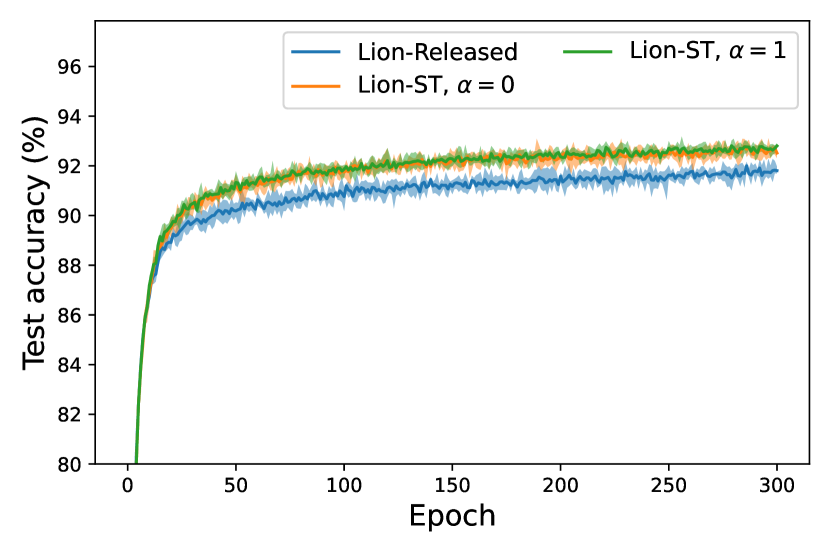
(a) Test accuracy, CIFAR-10

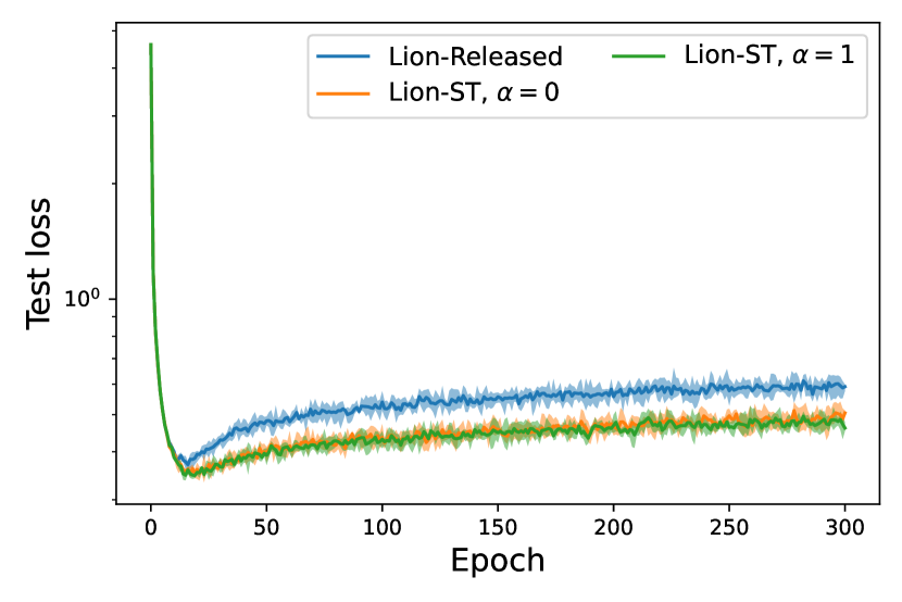
(b) Test loss, CIFAR-10

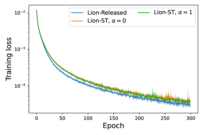
(c) Training loss, CIFAR-10

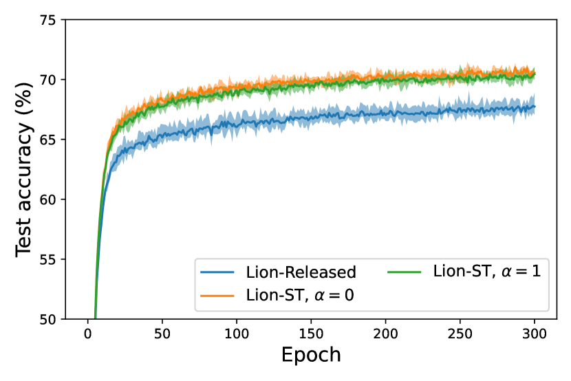
(d) Test accuracy, CIFAR-100

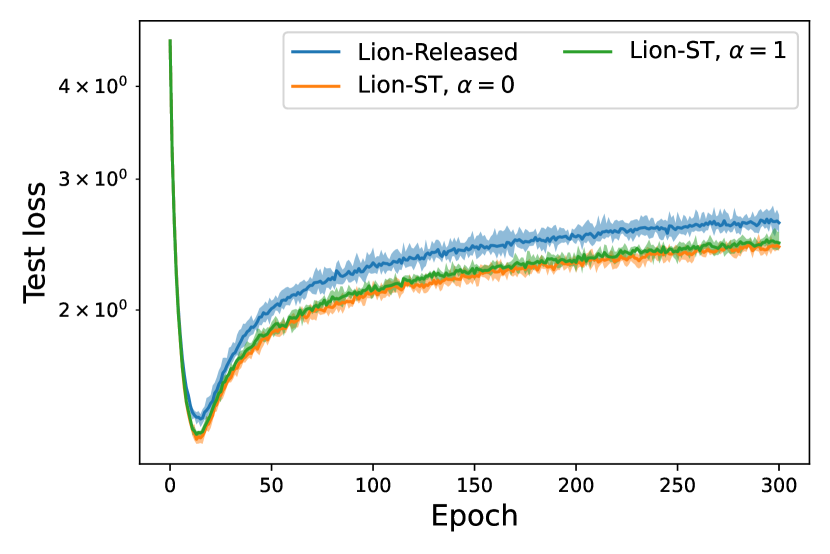
(e) Test loss, CIFAR-100

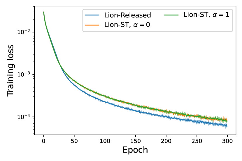
(f) Training loss, CIFAR-100

Figure 1: Test results on applying the Lion method for training ResNet50 on CIFAR-10 and CIFAR-100 datasets. Here the “Lion-Released“ refers to the released version of the Lion method, where $\theta_{k}$ is fixed as a constant. “ST” is the abbreviation for “single-timescale”.

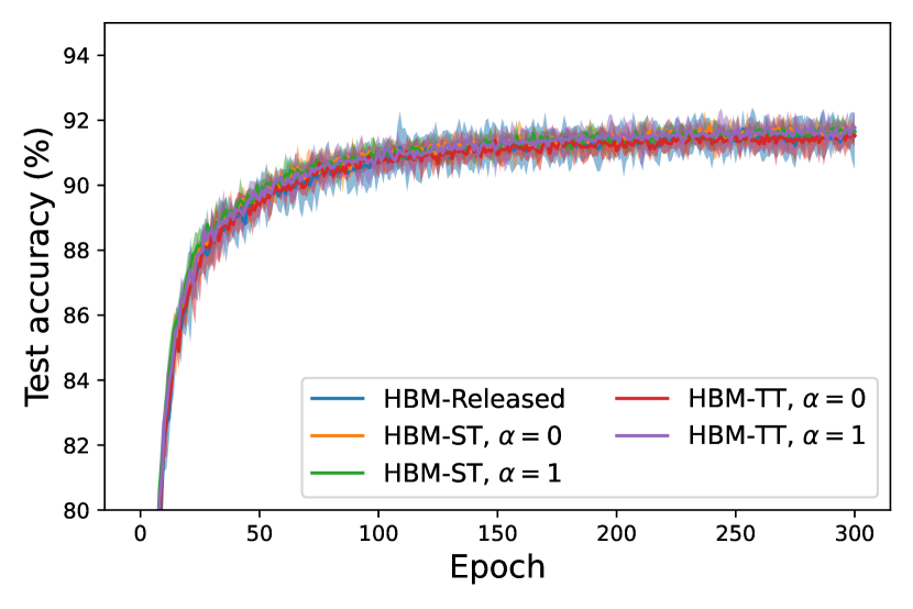
(a) Test accuracy, CIFAR-10

(b) Test loss, CIFAR-10

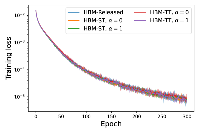
(c) Training loss, CIFAR-10

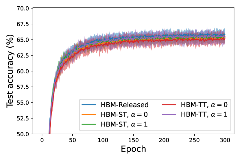
(d) Test accuracy, CIFAR-100

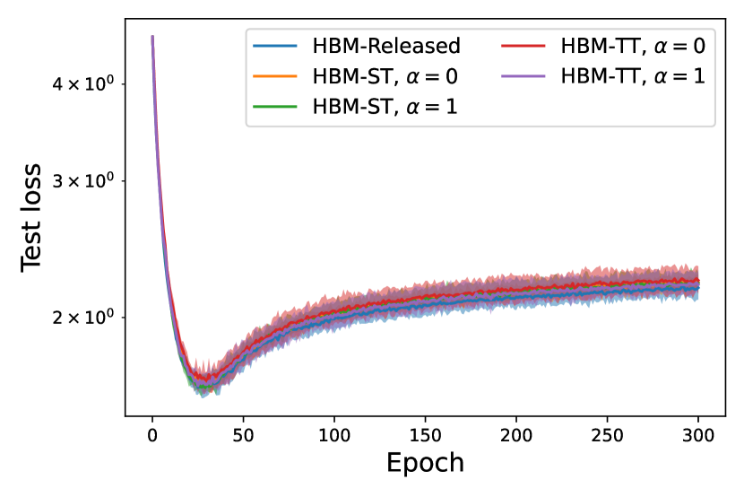
(e) Test loss, CIFAR-100

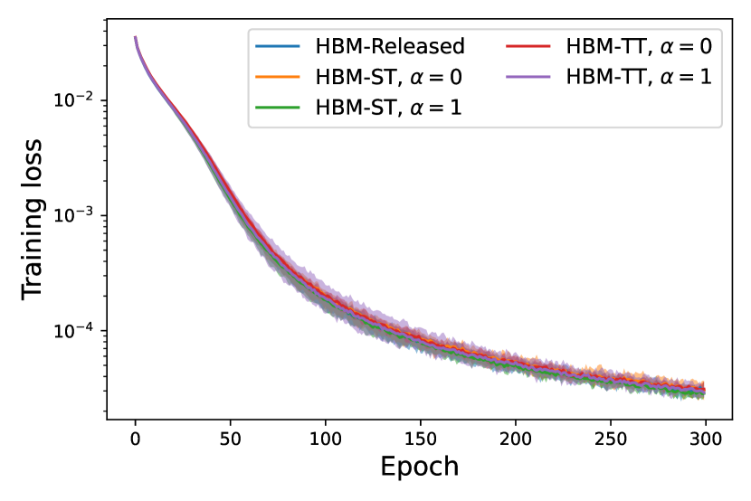
(f) Training loss, CIFAR-100

Figure 2: Test results on applying heavy-ball SGD method (HBM) for training ResNet50 on CIFAR-10 and CIFAR-100 datasets. Here “HBM-Released” refers to the released version of HBM, where $\theta_{k}$ is fixed as a constant. “ST” and “TT” are the abbreviations for “single-timescale” and “two-timescale”, respectively.

We evaluate the numerical performance of Algorithm 1 by comparing it with previously released SGD-type methods in the community, including Lion and heavy-ball SGD. It is important to note that these previously released SGD-type methods can be regarded as Algorithm 1 with a fixed $\theta_{k}=\theta_{0}$ throughout the iterations. On the other hand, as discussed in Section 3.2, our analysis enables the sequences of stepsizes $\{\eta_{k}\}$ and $\{\theta_{k}\}$ to diminish in the rate of $o(1/\log(k))$, which almost remains constant throughout the iterations.

Therefore, in our numerical experiments, we focus on testing the numerical performance of Algorithm 1 with the stepsizes $\{\eta_{k}\}$ and $\{\theta_{k}\}$ that diminish more rapidly than the rate of $o(1/\log(k))$, for a better illustration of its efficiency. We test the performance of the compared SGD-type methods for training ResNet-50 [21] on image classification tasks using the CIFAR-10 and CIFAR-100 datasets [24]. The batch size is set to 128 for all test instances.

For those previously released SGD-type methods in the community, in $k$-th epoch, the stepsize is selected as $\eta_{k}=\frac{\eta_{0}}{\sqrt{k+1}}$ and $\theta_{k}=\tau\eta_{0}$. The values of $\eta_{0}$ and $\tau$ are determined through a grid search following the approach in [14]. We consider $\eta_{0}$ from the set $\{k_{1}\times 10^{-k_{2}}:k_{1}=1,3,5,7,9,~{}k_{2}=3,4,5\}$, and $\tau$ from $\{0.1/\eta_{0},0.05/\eta_{0},0.01/\eta_{0},0.005/\eta_{0},0.001/\eta_{0}\}$. The goal is to find the combination of $(\eta_{0},\tau)$ that yields the most significant accuracy improvement after 20 epochs. The other parameters for the previously released SGD-type methods remain fixed at their default values.

For our proposed single-timescale SGD-type methods (Algorithm 1 with $\theta_{k}=\tau\eta_{k}$ for any $k\geq 0$), we keep the consistency in all parameters with those utilized in previously released SGD-type methods. Furthermore, for our proposed two-timescale SGD-type methods, we choose $\theta_{k}=\sqrt{\eta_{k}}$ for any $k\geq 0$. Additionally, to assess the performance of our proposed SGD-type methods with Nesterov momentum, we conduct experiments where Algorithm 1 is tested with two distinct parameter values of $\alpha$. Each test instance is executed five times with varying random seeds. In each test instance, all compared SGD-type methods employ the same random seed and are initialized with the same randomly generated initial points generated by PyTorch’s default initialization function.

Figure 1 and Figure 2 illustrate the performance of our proposed SGD-type methods that employ diminishing $\theta_{k}$, together with comparisons to their existing well-established versions that fix $\theta_{k}=\theta_{0}$. These empirical results highlight the effectiveness of our proposed SGD-type methods, as they achieve comparable performance to their well-established counterparts in the community. Furthermore, we observe that with single-timescale stepsizes, the Lion method attains higher test accuracy and lower test loss as compared to its well-established counterpart that fixes $\theta_{k}$ as a constant. These findings demonstrate that by selecting ${\theta_{k}}$ as a diminishing sequence within existing SGD-type methods, we can preserve their practical performance while benefiting from the convergence guarantees provided by our proposed framework.

7 Conclusion

In this paper, we propose a novel framework (GSGD) for SGD-type methods in nonsmooth optimization, especially in the context of training nonsmooth neural networks. With mild assumptions that are applicable to most deep learning tasks, we establish the convergence properties of our proposed framework (GSGD) with single-timescale stepsizes. For two-timescale stepsizes, we establish the convergence for heavy-ball SGD method under mild conditions. In addition, we provide a counter-example illustrating that two-timescale signSGD and Lion may fail to converge, even under noiseless settings. We demonstrate that our proposed framework encompasses some popular SGD-type methods such as heavy-ball SGD, SignSGD, Lion, and normalized SGD. Furthermore, when the objective function $f$ takes a finite-sum formulation, we prove that these SGD-type methods converge to stationary points of $f$ in both senses of the conservative field and the Clarke subdifferential, under mild conditions. Our numerical experiments demonstrate that SGD-type methods when equipped with single-timescale or two-timescale stepsizes, achieve comparable efficiency to their released counterparts in the research community, where the parameter $\theta_{k}$ is fixed as a constant throughout the iterations. The results in this paper provide theoretical guarantees for the performance of SGD-type methods in the realm of nonsmooth nonconvex optimization, especially in the training of nonsmooth neural networks that are differentiated by automatic differentiation algorithms.

References

- [1] Felipe Alvarez, Hedy Attouch, Jérôme Bolte, and Patrick Redont. A second-order gradient-like dissipative dynamical system with hessian-driven damping.: Application to optimization and mechanics. Journal de mathématiques pures et appliquées, 81(8):747–779, 2002.
- [2] F Alvarez D and JM Pérez C. A dynamical system associated with newton’s method for parametric approximations of convex minimization problems. Applied Mathematics and Optimization, 38(2):193–217, 1998.
- [3] Marcin Andrychowicz, Misha Denil, Sergio Gomez, Matthew W Hoffman, David Pfau, Tom Schaul, Brendan Shillingford, and Nando De Freitas. Learning to learn by gradient descent by gradient descent. Advances in neural information processing systems, 29, 2016.
- [4] Michel Benaïm, Josef Hofbauer, and Sylvain Sorin. Stochastic approximations and differential inclusions. SIAM Journal on Control and Optimization, 44(1):328–348, 2005.
- [5] Jeremy Bernstein, Yu-Xiang Wang, Kamyar Azizzadenesheli, and Animashree Anandkumar. Signsgd: Compressed optimisation for non-convex problems. In International Conference on Machine Learning, pages 560–569. PMLR, 2018.
- [6] Pascal Bianchi, Walid Hachem, and Sholom Schechtman. Convergence of constant step stochastic gradient descent for non-smooth non-convex functions. Set-Valued and Variational Analysis, pages 1–31, 2022.
- [7] Pascal Bianchi and Rodolfo Rios-Zertuche. A closed-measure approach to stochastic approximation. arXiv preprint arXiv:2112.05482, 2021.
- [8] Edward Bierstone and Pierre D Milman. Semianalytic and subanalytic sets. Publications Mathématiques de l’IHÉS, 67:5–42, 1988.
- [9] Jérôme Bolte, Aris Daniilidis, Adrian Lewis, and Masahiro Shiota. Clarke subgradients of stratifiable functions. SIAM Journal on Optimization, 18(2):556–572, 2007.
- [10] Jérôme Bolte and Edouard Pauwels. A mathematical model for automatic differentiation in machine learning. Advances in Neural Information Processing Systems, 33:10809–10819, 2020.
- [11] Jérôme Bolte and Edouard Pauwels. Conservative set valued fields, automatic differentiation, stochastic gradient methods and deep learning. Mathematical Programming, 188(1):19–51, 2021.
- [12] Jérôme Bolte, Edouard Pauwels, and Rodolfo Rios-Zertuche. Long term dynamics of the subgradient method for lipschitz path differentiable functions. Journal of the European Mathematical Society, 2022.
- [13] Vivek S Borkar. Stochastic approximation: a dynamical systems viewpoint, volume 48. Springer, 2009.
- [14] Camille Castera, Jérôme Bolte, Cédric Févotte, and Edouard Pauwels. An inertial newton algorithm for deep learning. The Journal of Machine Learning Research, 22(1):5977–6007, 2021.
- [15] Xiangning Chen, Chen Liang, Da Huang, Esteban Real, Kaiyuan Wang, Yao Liu, Hieu Pham, Xuanyi Dong, Thang Luong, Cho-Jui Hsieh, et al. Symbolic discovery of optimization algorithms. arXiv preprint arXiv:2302.06675, 2023.
- [16] Frank H Clarke. Optimization and nonsmooth analysis, volume 5. SIAM, 1990.
- [17] Ashok Cutkosky and Harsh Mehta. Momentum improves normalized SGD. In International conference on machine learning, pages 2260–2268. PMLR, 2020.
- [18] Damek Davis, Dmitriy Drusvyatskiy, Sham Kakade, and Jason D Lee. Stochastic subgradient method converges on tame functions. Foundations of Computational Mathematics, 20(1):119–154, 2020.
- [19] John C Duchi and Feng Ruan. Stochastic methods for composite and weakly convex optimization problems. SIAM Journal on Optimization, 28(4):3229–3259, 2018.
- [20] Mert Gürbüzbalaban, Andrzej Ruszczyński, and Landi Zhu. A stochastic subgradient method for distributionally robust non-convex and non-smooth learning. Journal of Optimization Theory and Applications, 194(3):1014–1041, 2022.
- [21] Kaiming He, Xiangyu Zhang, Shaoqing Ren, and Jian Sun. Deep residual learning for image recognition. In Proceedings of the IEEE conference on computer vision and pattern recognition, pages 770–778, 2016.
- [22] Xiaoyin Hu, Nachuan Xiao, Xin Liu, and Kim-Chuan Toh. A constraint dissolving approach for nonsmooth optimization over the Stiefel manifold. arXiv preprint arXiv:2205.10500, 2022.
- [23] Xiaoyin Hu, Nachuan Xiao, Xin Liu, and Kim-Chuan Toh. An improved unconstrained approach for bilevel optimization. arXiv preprint arXiv:2208.00732, 2022.
- [24] Alex Krizhevsky, Geoffrey Hinton, et al. Learning multiple layers of features from tiny images. 2009.
- [25] Tam Le. Nonsmooth nonconvex stochastic heavy ball. arXiv preprint arXiv:2304.13328, 2023.
- [26] Andrew L Maas, Awni Y Hannun, Andrew Y Ng, et al. Rectifier nonlinearities improve neural network acoustic models. In Proc. icml, volume 30, page 3. Atlanta, Georgia, USA, 2013.
- [27] Luke Metz, Niru Maheswaranathan, Jeremy Nixon, Daniel Freeman, and Jascha Sohl-Dickstein. Understanding and correcting pathologies in the training of learned optimizers. In International Conference on Machine Learning, pages 4556–4565. PMLR, 2019.
- [28] VI Norkin. Generalized-differentiable functions. Cybernetics, 16(1):10–12, 1980.
- [29] Boris T Polyak. Some methods of speeding up the convergence of iteration methods. Ussr computational mathematics and mathematical physics, 4(5):1–17, 1964.
- [30] Herbert Robbins and Sutton Monro. A stochastic approximation method. The annals of mathematical statistics, pages 400–407, 1951.
- [31] Andrzej Ruszczyński. Convergence of a stochastic subgradient method with averaging for nonsmooth nonconvex constrained optimization. Optimization Letters, 14(7):1615–1625, 2020.
- [32] Andrzej Ruszczynski. A stochastic subgradient method for nonsmooth nonconvex multilevel composition optimization. SIAM Journal on Control and Optimization, 59(3):2301–2320, 2021.
- [33] Lou Van den Dries and Chris Miller. Geometric categories and o-minimal structures. Duke Mathematical Journal, 84(2):497–540, 1996.
- [34] Alex J Wilkie. Model completeness results for expansions of the ordered field of real numbers by restricted Pfaffian functions and the exponential function. Journal of the American Mathematical Society, 9(4):1051–1094, 1996.
- [35] Nachuan Xiao, Xiaoyin Hu, Xin Liu, and Kim-Chuan Toh. Adam-family methods for nonsmooth optimization with convergence guarantees. arXiv preprint arXiv:2305.03938, 2023.
- [36] Nachuan Xiao, Xin Liu, and Kim-Chuan Toh. Dissolving constraints for Riemannian optimization. Mathematics of Operations Research, 2023.
- [37] Mengqi Xue, Jie Song, Xinchao Wang, Ying Chen, Xingen Wang, and Mingli Song. KDExplainer: A task-oriented attention model for explaining knowledge distillation. In Proceedings of the Thirtieth International Joint Conference on Artificial Intelligence, IJCAI-21, pages 3228–3234, 2021.
- [38] Yang You, Igor Gitman, and Boris Ginsburg. Large batch training of convolutional networks. arXiv preprint arXiv:1708.03888, 2017.
- [39] Yang You, Jing Li, Sashank Reddi, Jonathan Hseu, Sanjiv Kumar, Srinadh Bhojanapalli, Xiaodan Song, James Demmel, Kurt Keutzer, and Cho-Jui Hsieh. Large batch optimization for deep learning: Training bert in 76 minutes. arXiv preprint arXiv:1904.00962, 2019.
- [40] Bohang Zhang, Jikai Jin, Cong Fang, and Liwei Wang. Improved analysis of clipping algorithms for non-convex optimization. Advances in Neural Information Processing Systems, 33:15511–15521, 2020.
- [41] Jingzhao Zhang, Sai Praneeth Karimireddy, Andreas Veit, Seungyeon Kim, Sashank Reddi, Sanjiv Kumar, and Suvrit Sra. Why are adaptive methods good for attention models? Advances in Neural Information Processing Systems, 33:15383–15393, 2020.
- [42] Pan Zhou, Jiashi Feng, Chao Ma, Caiming Xiong, Steven Chu Hong Hoi, et al. Towards theoretically understanding why SGD generalizes better than Adam in deep learning. Advances in Neural Information Processing Systems, 33:21285–21296, 2020.