FaIRGP: A Bayesian Energy Balance Model
for Surface Temperatures Emulation

Abstract

Emulators, or reduced complexity climate models, are surrogate Earth system models that produce projections of key climate quantities with minimal computational resources. Using time-series modeling or more advanced machine learning techniques, data-driven emulators have emerged as a promising avenue of research, producing spatially resolved climate responses that are visually indistinguishable from state-of-the-art Earth system models. Yet, their lack of physical interpretability limits their wider adoption. In this work, we introduce FaIRGP, a data-driven emulator that satisfies the physical temperature response equations of an energy balance model. The result is an emulator that (i) enjoys the flexibility of statistical machine learning models and can learn from observations, and (ii) has a robust physical grounding with interpretable parameters that can be used to make inference about the climate system. Further, our Bayesian approach allows a principled and mathematically tractable uncertainty quantification. Our model demonstrates skillful emulation of global mean surface temperature and spatial surface temperatures across realistic future scenarios. Its ability to learn from data allows it to outperform energy balance models, while its robust physical foundation safeguards against the pitfalls of purely data-driven models. We also illustrate how FaIRGP can be used to obtain estimates of top-of-atmosphere radiative forcing and discuss the benefits of its mathematical tractability for applications such as detection and attribution or precipitation emulation. We hope that this work will contribute to widening the adoption of data-driven methods in climate emulation.

Journal of Advances in Modeling Earth Systems (JAMES)

Department of Statistics, University of Oxford, Oxford, UK School of CMS & AIML, University of Adelaide, Adelaide, Australia Scripps Institution of Oceanography and Halicioğlu Data Science Institute, University of California, San Diego, US

Shahine Bouabidshahine.bouabid@stats.ox.ac.uk

We introduce FaIRGP, a physically-informed Bayesian machine learning emulator for global and local mean surface temperatures.

The model outperforms both purely physically-driven and purely data-driven baseline emulators on several metrics across realistic future scenarios.

The model is fully mathematically tractable, which makes it a convenient and easy to use probabilistic tool for emulation of surface temperatures, but also for downstream applications such as detection and attribution or precipitation emulation.

Plain Language Summary

Emulators are simplified climate models that can be used to rapidly explore climate scenarios — they can run in less than a minute on an average computer. They are key tools used by the Intergovernmental Panel on Climate Change to explore the diversity of possible future climates. Data-driven emulators use advanced machine learning techniques to produce climate predictions that look very similar to the predictions of complex climate models. However, they are not easy to interpret, and therefore to trust in practice. In this work, we introduce FaIRGP, a data-driven emulator based on physics. The emulator is flexible and can learn from data to improve its predictions, but is also grounded on physical energy balance relationships, which makes it robust and interpretable. The model performs well in predicting future global and local temperatures under realistic future scenarios, outperforming purely physics-driven or purely data-driven models. Further, the probabilistic nature of our model allows for mathematically tractable uncertainty quantification. By gaining trust in such a data-driven yet physically grounded model, we hope the climate science community can benefit more widely from their potential.

1 Introduction

Earth system models (ESMs) [Flato (2011)] are key tools to understand current climate dynamics and climate change responses to greenhouse gas emissions. They constitute an extensive physical simulation of Earth’s atmosphere and ocean fluid dynamics, used for example in the Couple Model Intercomparison Project [Meehl . (2007), Taylor . (2012), Eyring . (2016)] to study past and future climate. As such, they offer the most comprehensive view of what future climate could look like. They are also used as an idealized fully controlled environment to study climate dynamics and understand its underlying drivers. In particular, they play a central role in the estimation of key properties of the climate system such as timescales and equilibrium responses to the change in carbon dioxide concentration in the atmosphere [Allen . (2009), Collins . (2014)] and the effect of aerosols [Levy . (2013)].

Running simulations with an ESM requires an astute understanding of the climate science background, of the numerical schemes used to simulate climate dynamics, and access to an adequate computational infrastructure. Therefore, only a limited number of research teams around the world can realistically afford to perform climate simulations. A direct consequence is that a variety of scientific applications relying on future climate projections — such as agricultural studies [Rosenzweig . (2014)], energy models [Turner . (2017)] or global socio-economic human models [Akhtar . (2013)] — must settle for publicly available precomputed climate projections that have been cherry-picked by climate scientists, and may not be tailored to the application needs. The need for expensive computational resources also serves as an important barrier, making it inaccessible for independent researchers and less well-equipped research teams to run experiments with ESMs. This exacerbates the already unequal representation in high-impact climate science research, where the global north is disproportionately represented [Tandon (2021)].

Furthermore, even when the resource needs are met to run experiments with an ESM, their computational cost remains a critical obstacle. Indeed, the uncertainty over the ESM parameterisation, the climate system internal variability and the emission pathway the world will choose, together span a high-dimensional uncertainty space. Therefore, obtaining a comprehensive coverage of this uncertainty requires running numerous climate simulations, which quickly meets computational cost limitations. As a result, much of the climate variability and potential socio-economic pathways remain in practice unexplored.

Together, these limitations have fostered the emergence of simpler surrogate ESMs which are inexpensive to compute and referred to as emulators. Unlike ESMs, emulators do not explicitly model the fluid dynamics of the atmosphere and oceans and focus on a limited number of climate features, such as surface temperatures or precipitations. They can run thousands of years of simulation in less than a minute on an average personal computer [Leach . (2021)], hence making accessible the emulation of climate projections under configurations unexplored by ESMs.

An important class of emulators are simple climate models (SCMs) [Meinshausen . (2011), Meinshausen . (2020), Millar . (2017), Smith . (2018), Leach . (2021)], which propose a reduced order representation of the climate system that describes the changes in global surface temperature through imbalances in Earth’s energy budget [Held . (2010)]. A well-established class of simple climate models are energy balance models (EBMs) [Meinshausen . (2011), Rypdal (2012), Geoffroy . (2013), Millar . (2017), Fredriksen  Rypdal (2017), Lovejoy . (2021)]. They represent the atmosphere-ocean system as a set of connected boxes forced by radiative flux at the top of the atmosphere. Whilst they constitute a drastic simplification of the climate system, EBMs are robust physically-motivated models, and therefore remain the main tool used to connect the IPCC working physical basis research [Masson-Delmotte . (2021)] with the adaptation and mitigation efforts [Pörtner . (2022)].

Another important class of emulators are data-driven emulators. In contrast to SCMs, they do not explicitly model forcing dynamics, and rather rely on statistical modelling techniques to emulate key climate variables such as temperature or precipitation [Del Rio Amador  Lovejoy (2019), Beusch . (20202), Link . (2019), Goodwin . (2020), Castruccio . (2014), Holden  Edwards (2010)]. Statistical modelling enjoys greater flexibility and has produced powerful emulators, capable of successfully approximating ESMs’ spatially resolved climate projections with visually indistinguishable outputs. More recently, statistically driven emulators drawing from advances in statistical machine learning have demonstrated a remarkable capacity at regressing global emission profiles onto spatially resolved temperature and precipitation maps [Watson-Parris . (2021)].

However, both SCMs and data-driven emulators display fundamental limitations. Whilst EBMs provide a robust physical framework to reason about the climate system, they remain a simplistic model which may display a poor fit to ESM’s outputs in certain scenarios [Meinshausen . (2011), Geoffroy . (2013), Jackson . (2022)] and can only operate at the global level. Reasoning only in terms of global mean temperatures fails to capture the difference in exposure of different world regions and limits use for scientific applications that require regional projections. On the other hand, data-driven emulators are also limited in their ability to provide a complete, reliable picture of the climate system. Indeed, their lack of robust physical grounding limits their capacity to make inference about the climate system [Beusch . (20202), Link . (2019)]. Further, the outputs from these emulators are often subject to qualitative evaluation and may not be trustworthy, in part because of limited understanding on how they might behave outside the observed data regimes.

In this work, we address these limitations by formulating a hybrid physical/statistical emulator that will both enjoy the robust physical grounding of SCMs, and the flexibility of statistical machine learning methods, thereby combining the advantages of both classes of emulators. We propose a probabilistic emulator for the task of reproducing an ESM temperature response to greenhouse gas and aerosols emissions. Our model builds upon a simple EBM, but places a Gaussian process (GP) prior over the radiative forcing, thereby inducing a stochastic temperature response model. We show that the resulting emulated temperature turns out to also be a GP, with a physically-informed covariance structure that reflects the dynamics of the EBM. In consequence, we can update the EBM with temperature data to learn a posterior distribution over global temperatures, but also over radiative forcing. Further, we demonstrate how our model can be easily extended to emulate spatially-resolved maps of annual surface temperatures.

Experiments demonstrate skilful prediction of global and spatial mean surface temperatures, with improvements over a simple EBM and over a simple GP model. We obtain robust predictions even when only training with historical data, or when predicting over scenarios outside the range of emissions of greenhouse gases and aerosols observed during training. Additionally, we show that the model improves over baselines to emulate temperature changes induced by anthropogenic aerosols emissions, and can provide useful estimates of the top-of-atmosphere radiative forcing.

2 Background

2.1 Energy Balance Models

Energy balance models (EBMs) [Sellers (1969), Holden  Edwards (2010)] are a lower-order representation of the climate system, where the changes in global temperature are explained by the imbalance in the Earth’s energy budget. The most common and established class of EBM are box models. They represent the atmosphere and ocean as a set of vertically stacked boxes, where the uppermost box is exposed to top-of-atmosphere radiative flux.

In a box model EBM, each box has a different heat capacity $C_{i}$, heat transfer coefficients $\kappa_{i}$ with the adjacent boxes, and its own temperature $T^{(i)}(t)$, as depicted in Figure 1. The uppermost box represents the fast components of the climate system, generally limited to the atmosphere, while the following boxes are used to represent slower components of the climate system such as shallow ocean and deep ocean.

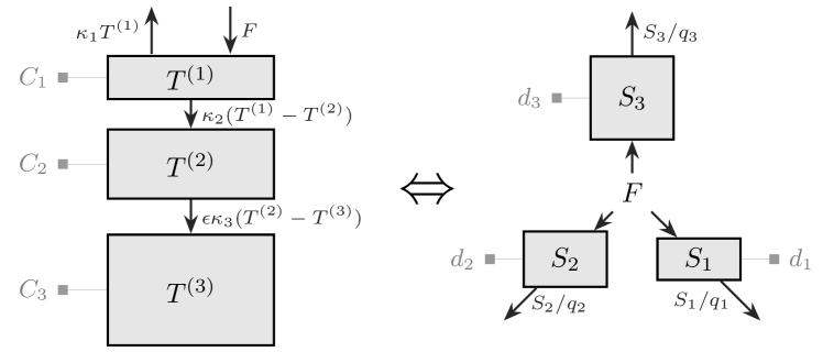
Figure 1: Schematic representation of $3$-box energy balance model, the arrows represent the flow of heat. Left: Temperature response model representation. Thicker boxes have a larger heat capacity (i.e. $C_{1}<C_{2}<C_{3}$) and the arrows represent the flow of heat. $\kappa_{1},\kappa_{2},\kappa_{3}$ are the heat transfer coefficients between the boxes and $\epsilon>0$ denotes the deep ocean heat uptake efficacy. Right: Thermal response model representation. Thicker boxes have larger response timescale (i.e. $d_{1}<d_{2}<d_{3}$).

Let ${\mathbf{X}}(t)=\begin{bmatrix}T^{(1)}(t)&\ldots&T^{(k)}(t)\end{bmatrix}^{\top}$ be the vector concatenation of the temperatures within the boxes in a model with $k$ boxes. The change in temperature of a $k$-box EBM is described by the following simple first order linear ordinary differential equation (ODE)

$$\frac{\,{\mathrm{d}}{\mathbf{X}}(t)}{\,{\mathrm{d}}t}={\mathbf{A}}{\mathbf{X}}(t)+{\mathbf{b}}F(t),$$ (1)

where ${\mathbf{A}}$ is a tridiagonal temperature feedback matrix that depends on heat capacities $C_{i}$, heat transfer coefficients $\kappa_{i}$, and deep ocean uptake efficacy $\varepsilon$, and ${\mathbf{b}}$ is a radiative forcing feedback vector given by

$${\mathbf{b}}=\begin{bmatrix}1/C_{1}&0&\ldots&0\end{bmatrix}^{\top}.$$ (2)

$F(t)$ denotes the top of atmosphere effective radiative forcing — radiative forcing for short — i.e. the change in energy flux caused by natural or anthropogenic factors of climate change. It is only applied to the surface box, i.e. the uppermost box.

Whilst physically motivated, box-models remain an abstract representation of the climate system. Therefore their parameters, such as boxes heat capacities, are not realistic quantities that can be calculated, but rather need to be tuned against data using calibration methods [Meinshausen . (2011), Millar . (2017)] or maximum likelihood strategies [Cummins . (2020)].

The simplest box models only use $k=2$ boxes, thereby splitting the climate system into 2 groups: fast and slow components. Whilst reductive, this split has proven to be a robust approximation of the climate system [Held . (2010)]. In fact, 2-box EBMs are today the primary tool used for linking the IPCC physical basis research [Masson-Delmotte . (2021)] with the adaptation and mitigation efforts [Pörtner . (2022)]. It is however worth noting recent advocacy for 3-box models [Leach . (2021)], highlighting the insufficiency of 2-box models to capture the full range of behaviour observed in CMIP6 models [Tsutsui (2020), Cummins . (2020)].

Table 1: Notation, description and unit of named parameters.

Notation	Unit	Description
$F(t)$	Wm-2	Effective top of atmosphere radiative forcing
$T^{(i)}(t)$	K	Temperature of the $i$th box
$C_{i}$	JK-1	Heat capacity of the $i$th box
$\kappa_{i}$	Wm-2K-1	Heat exchange coefficient of the $i$th box
$\varepsilon$	1	Deep ocean heat uptake efficacy
$T(t)$	K	Global mean surface temperature ($T^{(1)}(t)$)
$S_{i}(t)$	K	Response of the $i$th thermal box
$d_{i}$	years	Response timescale of $i$th thermal box
$q_{i}$	KW-1m2	Equilibrium response of $i$th thermal box
$\chi$	-	Atmospheric agent (e.g. CO2, SO2)
$E(t)$	-	Emission of agents in the atmosphere

2.2 Impulse response formulation

The main box of interest in a box-model is the uppermost box since it describes the global mean surface temperature response $T^{(1)}(t)$ to the radiative forcing $F(t)$. In general, computing $T^{(1)}(t)$ can be simplified by diagonalising the ODE (1). The result is an equivalent impulse response formulation of the temperature response model, depicted on the right in Figure 1, and referred to as the thermal response ODE [Millar . (2017)].

Let us rename the temperature of the first box as $T(t)$ for simplicity. Then, for a $k$-box model, the thermal response ODE is formally given by

$$\left\{\begin{aligned} \hfil\displaystyle\begin{split}&\frac{\,{\mathrm{d}}S_{i}(t)}{\,{\mathrm{d}}t}=\frac{1}{d_{i}}\left(q_{i}F(t)-S_{i}(t)\right),\quad 1\leq i\leq k\\ &T(t)=\sum_{i=1}^{k}S_{i}(t),\end{split}\end{aligned}\right.$$ (3)

where $S_{i}(t)$ is the $i$^th thermal response, $d_{i}$ is the $i$^th response timescale and $q_{i}$ is the $i$^th equilibrium response. Table 1 provides a brief description of named parameters and units.

The primary benefit of the impulse response formulation is that each thermal response ODE can be solved independently, thereby avoiding the intricacies of solving a coupled system of ODE. Further, the timescale and equilibrium parameters $d_{i}$ and $q_{i}$ can be expressed in terms of the original boxes heat capacities $C_{i}$ and heat transfer coefficients $\kappa_{i}$. Detailed derivations can be found in [Geoffroy . (2013)].

Throughout this work, we will use as a reference SCM FaIRv2.0.0 [Leach . (2021)] (for Finite amplitude Impulse Response), a recent update of a well established SCM [Millar . (2017), Smith . (2018)], that offers a minimal level of structural complexity. FaIRv2.0.0 is effectively composed of 3 submodels: a gas cycle model, which converts emissions to concentrations, a radiative forcing model, which converts concentrations to radiative forcing, and a temperature response model, which converts radiative forcing into temperatures. The temperature response model of FaIRv2.0.0 exactly corresponds to the impulse response EBM described in (3). We refer to reader to the work of leach2021fairv2 for a comprehensive presentation of FaIRv2.0.0. In the rest of the paper, we permit ourselves to drop the v.2.0.0 and will refer to the model as FaIR.

2.3 Gaussian processes

Gaussian processes (GPs) [Rasmussen  Williams (2005)] are a ubiquitous class of Bayesian priors over real-valued functions. They enjoy convenient closed-form expressions, principled uncertainty quantification, and cover a rich class of complex functions. As a result, they have been widely used in various nonlinear and nonparametric regression problems in geosciences [Camps-Valls . (2016)].

We say that a real-valued stochastic process function ${\mathsf{f}}(t)$ is a GP if any finite collection of its evaluations has a joint multivariate normal distribution. A GP ${\mathsf{f}}(t)$ is fully determined by its mean function $m(t)$ and covariance function $k(t,t^{\prime})$. Formally, we write

$${\mathsf{f}}(t)\sim{\operatorname{GP}}(m,k),$$ (4)

where the mean and covariance functions are defined as

$$m(t)={\mathbb{E}}[{\mathsf{f}}(t)],\qquad k(t,t^{\prime})=\operatorname{Cov}({\mathsf{f}}(t),{\mathsf{f}}(t^{\prime})).$$ (5)

$m(t)$ and $k(t,t^{\prime})$ are typically user-specified. The covariance function, commonly called kernel, is a positive definite bivariate function that computes a notion of similarity between $t$ and $t^{\prime}$. For example, a widely used family of kernels are the Matérn kernels [Stein (1999)], where the one-dimensional Matérn-1/2 kernel is given by

$$k(t,t^{\prime})=\sigma^{2}\exp\left(-\frac{|t-t^{\prime}|}{\ell}\right),$$ (6)

where $\sigma^{2}$ is a variance hyperparameter and $\ell$ a lengthscale hyperparameter. More broadly, kernels (and hence GPs) can also be defined over multidimensional inputs, for example by substituting $|t-t^{\prime}|$ by the Euclidean distance between input vectors. When each dimension has a different lengthscale hyperparameter, the kernel is referred to as an automatic relevance determination kernel [Rasmussen  Williams (2005), Chapter 5.1].

Let ${\mathbf{y}}=\begin{bmatrix}y_{1}&\ldots&y_{n}\end{bmatrix}^{\top}$ denote independent observations at inputs ${\mathbf{t}}=\begin{bmatrix}t_{1}&\ldots&t_{n}\end{bmatrix}^{\top}$ of the noisy observation process ${\mathsf{y}}={\mathsf{f}}(t)+\upvarepsilon$, where $\upvarepsilon\sim{\mathcal{N}}(0,\sigma^{2})$. It is possible to inform the GP with these observations, thereby updating the prior into a posterior. In particular, the posterior distribution gives rise to a posterior GP, with a posterior mean function $\bar{m}(t)$ and a posterior covariance function $\bar{k}(t,t^{\prime})$,

$${\mathsf{f}}(t)\mid{\mathbf{y}}\sim{\operatorname{GP}}(\bar{m},\bar{k}).$$ (7)

The posterior mean and covariance enjoy a closed-form expression given by

$$\bar{m}(t) =m(t)+k(t,{\mathbf{t}})({\mathbf{K}}+\sigma^{2}{\mathbf{I}}_{n})^{-1}({\mathbf{y}}-m({\mathbf{t}})),$$ (8)

$$\bar{k}(t,t^{\prime}) =k(t,t^{\prime})-k(t,{\mathbf{t}})({\mathbf{K}}+\sigma^{2}{\mathbf{I}}_{n})^{-1}k({\mathbf{t}},t),$$ (9)

where ${\mathbf{I}}_{n}$ denotes the identity matrix of size $n$, $k(t,{\mathbf{t}})=\begin{bmatrix}k(t,t_{1})&\ldots&k(t,t_{n})\end{bmatrix}$, $k({\mathbf{t}},t)=k(t,{\mathbf{t}})^{\top}$ and ${\mathbf{K}}=k({\mathbf{t}},{\mathbf{t}})=\begin{bmatrix}k(t_{i},t_{j})\end{bmatrix}_{1\leq i,j\leq n}$. C provides an illustrative example on GP regression. For many more details on GPs, we refer the reader to rasmussen2005gaussian.

3 FaIRGP

In this section, we present FaIRGP, a GP emulator for global mean surface temperature that leverages the thermal response model from FaIR. We begin by motivating a Bayesian treatment of the radiative forcing and formulate a GP prior over the forcing. We show this modification naturally results in a stochastic formulation of the thermal response model, which admits a GP with a physically-informed covariance structure for solution. In addition, we show how this framework can seamlessly account for the climate internal variability. Finally, we provide closed-form expressions for the posterior distributions over temperature and forcing, which can readily be used for emulation.

In what follows, we adopt the following notational conventions: deterministic variables are denoted with serif font ($Z$), stochastic variables are denoted with sans-serif font (${\mathsf{Z}}$) and vector/matrix versions are denoted in bold (${\mathbf{Z}}$, $\boldsymbol{\mathsf{Z}}$).

3.1 Radiative forcing as a Gaussian process

The top-of-atmosphere radiative forcing is the fundamental quantity used to describe Earth’s energy imbalance. The value of this forcing is primarily determined by the emissions of greenhouse gases and aerosols in the atmosphere. In FaIR, the radiative forcing term $F(t)$ drives the temperature response model (1). Having access to a reliable estimate of the forcing, and in particular to the forcing response to greenhouse gas and aerosol emissions, is therefore critical to produce trustworthy emulated temperatures.

Computing an accurate estimate of the radiative forcing requires modelling how greenhouse gases and aerosols interact with radiations in the atmosphere, accounting for atmospheric adjustments and uncertainty in the measured parameters which may further complicate the calculation. The intricacy of such task has lead to the development of forcing estimation methods which rely on simplifying assumptions. For example, in FaIR, the forcing model is formulated as a combination of logarithmic, linear and square-root terms of greenhouse gas and aerosols concentrations. Namely, let $\chi$ denote a given atmospheric agent (e.g. CO₂, CH₄, SO₂), the radiative forcing induced by $\chi$ is modeled as

$$F^{\chi}(t)=\alpha_{\log}^{\chi}\log\left(\frac{C^{\chi}(t)}{C_{0}^{\chi}}\right)+\alpha_{\mathrm{lin}}^{\chi}\left(C^{\chi}(t)-C_{0}^{\chi}\right)+\alpha_{\mathrm{sqrt}}^{\chi}\left(\sqrt{C^{\chi}(t)}-\sqrt{C_{0}^{\chi}}\right),$$ (10)

where $C^{\chi}(t)$ denotes the concentration in the atmosphere of agent $\chi$, $C_{0}^{\chi}$ the agent concentration at pre-industrial period and $\alpha_{\log}^{\chi},\alpha_{\mathrm{lin}}^{\chi},\alpha_{\mathrm{sqrt}}^{\chi}$ are scalar sensitivity coefficients. The total radiative forcing is then obtained by combining the contribution of each agent

$$F(t)=\sum_{\chi}F^{\chi}(t).$$ (11)

This choice of forcing model is motivated by studies of temperature and historical trajectories of these concentrations  [Manabe  Wetherald (1967), Forster . (2007), Myhre . (2014)], which have provided substantial evidence that the concentration-to-forcing relationship can be reasonably approximated by the combination of terms in (10). However, it is important to emphasise that (10) does not propose a robust physically-motivated model, but is rather more akin to statistical modelling, where the coefficients $\alpha_{\log}^{\chi},\alpha_{\mathrm{lin}}^{\chi},\alpha_{\mathrm{sqrt}}^{\chi}$ need to be fitted against climate model data. In fact, the values of the coefficients can vary substantially depending on the data used and the fitting procedure [Leach . (2021)].

Because the radiative forcing is a key driving quantity of the climate system, and therefore of the emulator, we argue it is critical to account for the uncertainty introduced by the FaIR model of radiative forcing. Specifically, this choice of simplified model of forcing reflects uncertainty caused by the lack of knowledge about the phenomenon we wish to describe, referred to as epistemic uncertainty [Hüllermeier  Waegeman (2021)]. We propose to account for this epistemic uncertainty over the forcing model through a Bayesian formalism, by placing a GP prior over the radiative forcing.

We propose to use the deterministic forcing function $F(t)$ as the mean function of our GP, thereby ensuring that our prior will behave in expectation like the FaIR forcing model. To model uncertainty, we introduce a covariance function $K(t,t^{\prime})$ acting over past emissions trajectories of the form

$$K(t,t^{\prime})=\rho\left(E(t),E(t^{\prime})\right),$$ (12)

where $E(t)=\begin{bmatrix}E^{\chi_{1}}(t)&\ldots&E^{\chi_{d}}(t)\end{bmatrix}^{\top}$ is a vector that represents emissions — or cumulative emissions — of atmospheric agents $\chi_{1},\ldots,\chi_{d}$ at a given time, and $\rho$ is a user-specified kernel. We assume throughout a simple Matérn-3/2 kernel with automatic relevance determination for $\rho$ and discuss more sophisticated options in Section 7. The prior we specify over the forcing is then formally defined by

$${\mathsf{F}}(t)\sim{\operatorname{GP}}(F,K),$$ (13)

where we emphasise that ${\mathsf{F}}(t)$ is now a stochastic process by using a sans-serif notation. This Bayesian formulation therefore directly hinges on the forcing model from (10), but introduces a notion of uncertainty quantification, thereby accounting for the epistemic uncertainty over the forcing response.

3.2 Thermal response model with GP forcing

We will now show that by combining the GP prior over the radiative forcing and the FaIR thermal response model, we obtain a GP prior over temperatures, which we name FaIRGP. Recall the thermal impulse response model presented in Section 2.2, described by a system of $k$ independent linear first order ODEs

$$\frac{\,{\mathrm{d}}S_{i}(t)}{\,{\mathrm{d}}t}=\frac{1}{d_{i}}(q_{i}F(t)-S_{i}(t)),$$ (14)

where the thermal responses $S_{i}(t)$ are such that $T(t)=\sum_{i=1}^{k}S_{i}(t)$ is the global mean surface temperature.

We propose to substitute the deterministic forcing function $F(t)$ in (14) by its Bayesian counterpart ${\mathsf{F}}(t)$. In doing so, we naturally induce a stochastic version of the thermal impulse response model. Namely, the resulting $i$^th stochastic thermal response, which we denote ${\mathsf{S}}_{i}(t)$, will satisfy the linear stochastic differential equation (SDE) given by

$$\,{\mathrm{d}}{\mathsf{S}}_{i}(t)=\frac{1}{d_{i}}(q_{i}{\mathsf{F}}(t)-{\mathsf{S}}_{i}(t))\,{\mathrm{d}}t.$$ (15)

The resolution of this thermal response SDE is similar to the resolution of the thermal response ODE. Namely, assuming ${\mathsf{S}}_{i}(0)=0$ at pre-industrial time, the solution to (15) takes the canonical form

$${\mathsf{S}}_{i}(t)=\frac{q_{i}}{d_{i}}\int_{0}^{t}{\mathsf{F}}(s)e^{-(t-s)/d_{i}}\,{\mathrm{d}}s.$$ (16)

However, the solution is now a stochastic process. Specifically, because GPs are stable under linear transformations, ${\mathsf{S}}_{i}(t)$ must also be a GP, with a mean and covariance function shaped by the form of this linear transformation. In our case, the linear transformation is given by the convolution operator with the exponential function in (16).

Therefore, the $i$^th thermal response can be characterised as a GP with the following mean and covariance functions

$$\left\{\begin{aligned} \hfil\displaystyle\begin{split}&{\mathsf{S}}_{i}(t)\sim{\operatorname{GP}}(m_{i},k_{ii})\\ &m_{i}(t)=\frac{q_{i}}{d_{i}}\int_{0}^{t}F(s)e^{-(t-s)/d_{i}}\,{\mathrm{d}}s\\ &k_{ii}(t,t^{\prime})=\left(\frac{q_{i}}{d_{i}}\right)^{2}\int_{0}^{t}\int_{0}^{t^{\prime}}K(s,s^{\prime})e^{-(t-s)/d_{i}}e^{-(t^{\prime}-s^{\prime})/d_{i}}\,{\mathrm{d}}s\,{\mathrm{d}}s^{\prime}.\end{split}\end{aligned}\right.$$ (17)

We observe that the mean function $m_{i}(t)$ exactly corresponds to the solution of the deterministic thermal response ODE (14). Hence, similarly to the GP forcing ${\mathsf{F}}(t)$, the GP thermal response ${\mathsf{S}}_{i}(t)$ will behave in expectation like the FaIR thermal response model. Further, the covariance $k_{ii}(t,t^{\prime})$ is expressed as a function of the forcing prior covariance $K$, but also of the parameters of the EBM, $d_{i}$ and $q_{i}$. As such, $k_{ii}(t,t^{\prime})$ defines a physically-informed covariance structure that propagates the uncertainty over the forcing ${\mathsf{F}}(t)$ — specified by our Bayesian prior — into uncertainty over the thermal response ${\mathsf{S}}_{i}(t)$.

If we now define the global mean surface temperature as the sum of thermal response GPs ${\mathsf{T}}(t)=\sum_{i=1}^{k}{\mathsf{S}}_{i}(t)$, then we can show that ${\mathsf{T}}(t)$ must also be a GP. Namely, let us define the cross-covariance function between thermal responses ${\mathsf{S}}_{i}(t)$ and ${\mathsf{S}}_{j}(t^{\prime})$ as

$$k_{ij}(t,t^{\prime}):=\operatorname{Cov}({\mathsf{S}}_{i}(t),{\mathsf{S}}_{j}(t^{\prime}))=\frac{q_{i}q_{j}}{d_{i}d_{j}}\int_{0}^{t}\int_{0}^{t^{\prime}}K(s,s^{\prime})e^{-(t-s)/d_{i}}e^{-(t^{\prime}-s^{\prime})/d_{j}}\,{\mathrm{d}}s\,{\mathrm{d}}s^{\prime}.$$ (18)

Then, the global mean surface temperature is a GP specified by the following mean and covariance functions

$$\left\{\begin{aligned} \hfil\displaystyle\begin{split}&{\mathsf{T}}(t)\sim{\operatorname{GP}}(m_{\mathsf{T}},k_{\mathsf{T}}),\\ &m_{\mathsf{T}}(t)=\sum_{i=1}^{k}m_{i}(t),\\ &k_{\mathsf{T}}(t,t^{\prime})=\sum_{i=1}^{k}\sum_{j=1}^{k}k_{ij}(t,t^{\prime}).\end{split}\end{aligned}\right.$$ (19)

By specifying a GP prior over the radiative forcing, we have obtained a GP prior over the temperature that uses the FaIR thermal response model as its backbone, which we name FaIRGP. Using FaIRGP serves as a principled measure of epistemic uncertainty over the emulator design. In particular, the integral form of its covariance function allows to account for past trajectories, thereby capturing the climate system memory effect, and producing robust uncertainty estimates. In addition, as we will see in Section 3.4, FaIRGP can go beyond a standard impulse response model by learning from data using standard GP regression techniques.

We emphasise that whilst we abuse notations for conciseness, the forcing prior ${\mathsf{F}}(t)$ is effectively a function of emissions (or cumulative emissions) through its covariance function $\rho\left(E(t),E(t^{\prime})\right)$. Therefore, ${\mathsf{T}}(t)$ is also a function of emissions, and its covariance function can be understood as “$k_{\mathsf{T}}\left(E(t),E(t^{\prime})\right)$”.

3.3 Accounting for climate internal variability

An important component of the climate system is its internal variability, which integrates the effects of weather phenomena — typically operating on the scale of days — into elements of the climate system, such as the ocean, cryosphere and land vegetation — which rather operate on the scale of months, years or decades [Hasselmann (1976)].

The climate internal variability can classically be modeled in a $k$-box model by introducing a white noise forcing disturbance over the uppermost box, i.e. the atmosphere box [Cummins . (2020)]. Formally, let ${\mathsf{B}}(t)$ be the standard one-dimensional Brownian motion and let $\boldsymbol{\mathsf{X}}(t)$ denote a stochastic version of the $k$-box model temperatures from (1). The temperature response model with internal variability is given by

$$\,{\mathrm{d}}\boldsymbol{\mathsf{X}}(t)={\mathbf{A}}\boldsymbol{\mathsf{X}}(t)\,{\mathrm{d}}t+{\mathbf{b}}F(t)\,{\mathrm{d}}t+\sigma{\mathbf{b}}\,{\mathrm{d}}{\mathsf{B}}(t),$$ (20)

where $\sigma>0$ is a variance term that controls the amplitude of the white noise, and we recall that ${\mathbf{b}}$ has zero everywhere but its first entry, therefore the white noise disturbance is only applied to the uppermost box. When the radiative forcing $F(t)$ is deterministic, this is equivalent to adding red noise onto the global mean surface temperature, or equivalently, modelling it as an Ornstein-Uhlenbeck process. The corresponding diagonalised impulse response system is given by

$$\,{\mathrm{d}}{\mathsf{S}}_{i}(t)=\frac{1}{d_{i}}\left(q_{i}F(t)-{\mathsf{S}}_{i}(t)\right)\,{\mathrm{d}}t+\sigma\frac{q_{i}}{d_{i}}\,{\mathrm{d}}{\mathsf{B}}(t),$$ (21)

where derivations are detailed in Appendix A.3. If we now again substitute the deterministic forcing $F(t)$ with the GP forcing ${\mathsf{F}}(t)$, it turns out that the long time regime solution to this stochastic impulse response system can be expressed as

$${\mathsf{S}}_{i}(t)\sim{\operatorname{GP}}(m_{i},k_{ii}+\sigma^{2}\gamma_{i}),$$ (22)

where $\gamma_{i}(t,t^{\prime})$ is an exponential, or Matérn-1/2, kernel function given by

$$\gamma_{i}(t,t^{\prime})=\frac{q_{i}^{2}}{2d_{i}}\exp\left(-\frac{|t-t^{\prime}|}{d_{i}}\right).$$ (23)

Therefore, FaIRGP can easily model the internal variability of the climate system simply by modifying its covariance structure. We observe that accounting for internal variability essentially corresponds to adding an independent autocorrelated noise process $\upeta_{i}(t)\sim{\operatorname{GP}}(0,\sigma^{2}\gamma_{i})$ to the thermal response GP obtained in (17).

Ultimately, we sum the thermal response together to obtain a surface temperature GP ${\mathsf{T}}(t)=\sum_{i=1}^{k}{\mathsf{S}}_{i}(t)$, which in the long time regime takes the form

$$\left\{\begin{aligned} \hfil\displaystyle\begin{split}&{\mathsf{T}}(t)\sim{\operatorname{GP}}\left(m_{\mathsf{T}},k_{\mathsf{T}}+\sigma^{2}\gamma_{\mathsf{T}}\right)\\ &\gamma_{\mathsf{T}}(t,t^{\prime})=\sum_{i=1}^{k}\nu_{i}\gamma_{i}(t,t^{\prime}),\end{split}\end{aligned}\right.$$ (24)

where $\nu_{i}$ is a dimensionless weight determined by $q_{i},d_{i}$ which accounts for cross-covariances between thermal responses internal variabilities. Its detailed expression can be found in Appendix A.3. Therefore, we can account for the climate internal variability simply by adding an independent noise process $\upeta_{\mathsf{T}}(t)=\sum_{i=1}^{k}\upeta_{i}(t)\sim{\operatorname{GP}}(0,\sigma^{2}\gamma_{\mathsf{T}})$ to the temperature response GP obtained in (19).

3.4 Posterior distribution over temperature and radiative forcing

In FaIRGP, the surface temperature response and the radiative forcing model can both be informed by global temperature observations. Using standard GP regression techniques [Rasmussen  Williams (2005)], FaIRGP can learn from data how to deviate from its backbone impulse response model to best account for actual temperature observations. The resulting model can then be used to emulate future temperatures, benefiting from both the robustness of its prior, and the flexibility of GP regression. As we will demonstrate it in Section 5, we can inform FaIRGP with historical observations and climate model data.

Assume we are under a fixed emission scenario e.g. working with historical emissions only. For observation times $t_{1}<\ldots<t_{n}$, suppose we observe global mean surface temperatures $T_{1},\ldots,T_{n}$, and also have access to greenhouse gas and aerosols emissions data $E_{1},\ldots,E_{n}\in{\mathbb{R}}^{d}$, where $d$ corresponds to the number of atmospheric agents $\chi_{1},\ldots,\chi_{d}$. We concatenate these observations into ${\mathbf{t}}=\begin{bmatrix}t_{1}&\ldots&t_{n}\end{bmatrix}^{\top}$, ${\mathbf{E}}=\begin{bmatrix}E_{1}&\ldots&E_{n}\end{bmatrix}^{\top}$ and ${\mathbf{T}}=\begin{bmatrix}T_{1}&\ldots&T_{n}\end{bmatrix}^{\top}$.

With notation abuse, the kernel $k_{\mathsf{T}}$ effectively evaluates the covariance between times $t_{i}$ and $t_{j}$ of the FaIRGP prior following $k_{\mathsf{T}}(t_{i},t_{j})=k_{\mathsf{T}}(E_{i},E_{j})$ because the forcing prior kernel $\rho$ is a function of emissions. The internal variability kernel $\gamma_{\mathsf{T}}$ evaluates the covariance between times $t_{i}$ and $t_{j}$ of the additive variability component following $\gamma_{\mathsf{T}}(t_{i},t_{j})$. We can therefore define the Gram matrices induced by $k_{\mathsf{T}}$ and $\gamma_{\mathsf{T}}$ over ${\mathbf{E}}$ and ${\mathbf{t}}$, i.e.

$${\mathbf{K}} =k_{\mathsf{T}}({\mathbf{E}},{\mathbf{E}})=\begin{bmatrix}k_{\mathsf{T}}(E_{i},E_{j})\end{bmatrix}_{1\leq i,j\leq n}$$ (25)

$${\boldsymbol{\Gamma}} =\gamma_{\mathsf{T}}({\mathbf{t}},{\mathbf{t}})=\begin{bmatrix}\gamma_{{\mathsf{T}}}(t_{i},t_{j})\end{bmatrix}_{1\leq i,j\leq n}.$$ (26)

Using these Gram matrices, we can update our prior over ${\mathsf{T}}(t)$ with observations to obtain a posterior GP over global mean surface temperatures given by

$${\mathsf{T}}(t)\mid{\mathbf{T}}\sim{\operatorname{GP}}(\bar{m}_{\mathsf{T}},\bar{k}_{\mathsf{T}}),$$ (27)

where the posterior mean $\bar{m}_{\mathsf{T}}(t)$ and the posterior covariance $\bar{k}_{\mathsf{T}}(t,t^{\prime})$ have the following closed-form expressions

$$\underbrace{\bar{m}_{\mathsf{T}}(t)}_{\text{posterior mean}} =\underbrace{m_{\mathsf{T}}(t)}_{\text{prior mean}}\!\!+\,\,\,\underbrace{k_{\mathsf{T}}(t,{\mathbf{t}})({\mathbf{K}}+\sigma^{2}{\boldsymbol{\Gamma}})^{-1}({\mathbf{T}}-m_{\mathsf{T}}({\mathbf{t}}))}_{\text{posterior correction}}$$ (28)

$$\underbrace{\bar{k}_{\mathsf{T}}(t,t^{\prime})}_{\text{posterior covariance}} =\underbrace{k_{\mathsf{T}}(t,t^{\prime})}_{\text{prior covariance}}\!\!\!-\,\,\,\underbrace{k_{\mathsf{T}}(t,{\mathbf{t}})({\mathbf{K}}+\sigma^{2}{\boldsymbol{\Gamma}})^{-1}k_{\mathsf{T}}({\mathbf{t}},t)}_{\text{posterior correction}}.$$ (29)

The posterior mean $\bar{m}_{\mathsf{T}}(t)$ explicitly corrects the prior mean $m_{\mathsf{T}}(t)$, which exactly corresponds to the FaIR deterministic temperature response $T(t)$. The correction introduced by the posterior mean in (28) is a data-driven deviation term, informed by the observed temperatures ${\mathbf{T}}$, observation times ${\mathbf{t}}$ and emissions in the matrix ${\mathbf{K}}$. A data-corrected uncertainty quantification is similarly provided by the posterior covariance $\bar{k}_{\mathsf{T}}(t,t^{\prime})$.

This posterior can then be used to emulate temperatures by making prediction at future time steps. A major interest of this formulation is that whilst the emulator hinges on robustness of the energy balance model for its prior, it can also benefit from the flexibility of GP regression by informing it with data in its posterior, thereby going beyond a simple impulse response model. In addition, the GP approach enjoys full probabilistic tractability, and detailed analytical expression of the posterior probability distribution are provided in Appendix A.4.

Similarly, we can also update the radiative forcing with observations of temperatures to formulate a posterior distribution over the forcing. Indeed, because the radiative forcing ${\mathsf{F}}(t)$ is also GP, it is jointly Gaussian with the temperature ${\mathsf{T}}(t)$. Namely, we can define a cross-covariance function as

$$k_{{\mathsf{F}}{\mathsf{T}}}(t,t^{\prime}):=\operatorname{Cov}({\mathsf{F}}(t),{\mathsf{T}}(t^{\prime}))=\sum_{i=1}^{k}\frac{q_{i}}{d_{i}}\int_{0}^{t^{\prime}}K(t,s^{\prime})e^{-(t^{\prime}-s^{\prime})/d_{i}}\,{\mathrm{d}}s^{\prime}.$$ (30)

Therefore, it is also possible to update our prior over ${\mathsf{F}}(t)$, resulting in a posterior distribution over the radiative forcing given by

$$\left\{\begin{aligned} \hfil\displaystyle\begin{split}&{\mathsf{F}}(t)\mid{\mathbf{T}}\sim{\operatorname{GP}}(\bar{m}_{\mathsf{F}},\bar{k}_{\mathsf{F}})\\ &\bar{m}_{\mathsf{F}}(t)=F(t)+k_{{\mathsf{F}}{\mathsf{T}}}(t,{\mathbf{t}})({\mathbf{K}}+\sigma^{2}{\boldsymbol{\Gamma}})^{-1}({\mathbf{T}}-m_{\mathsf{T}}({\mathbf{t}}))\\ &\bar{k}_{\mathsf{F}}(t,t^{\prime})=K(t,t^{\prime})-k_{{\mathsf{F}}{\mathsf{T}}}(t,{\mathbf{t}})({\mathbf{K}}+\sigma^{2}{\boldsymbol{\Gamma}})^{-1}k_{{\mathsf{F}}{\mathsf{T}}}(t,{\mathbf{t}})^{\top}.\end{split}\end{aligned}\right.$$ (31)

By updating the radiative forcing with observations of temperatures, we obtain an estimates of the forcing that corrects for the observations ${\mathbf{T}}$. Like for temperatures, the posterior mean $\bar{m}_{\mathsf{F}}(t)$ corrects the FaIR forcing model $F(t)$ with a data-informed inductive bias, and corresponding uncertainty quantification provided by the posterior covariance $\bar{k}_{\mathsf{F}}(t,t^{\prime})$. Further, we can verify that solving the thermal response SDE for the posterior forcing ${\mathsf{F}}(t)\mid{\mathbf{T}}$ yields the posterior temperature ${\mathsf{T}}(t)\mid{\mathbf{T}}$ as the solution. Therefore, the forcing posterior and the temperature posterior are consistent with each other.

Finally, we note that access to a closed-form probability density for the prior allows us to tune the model parameters using a maximum likelihood strategy. Specifically, we may want to tune model parameters such as the internal variability magnitude $\sigma$, parameters of the prior kernel $K(t,t^{\prime})$, but also FaIR parameters such as $d_{i}$, $q_{i}$ or the forcing model coefficients $\alpha_{\log}^{\chi},\alpha_{\mathrm{lin}}^{\chi},\alpha_{\mathrm{sqrt}}^{\chi}$. This can be achieved by using for example a stochastic gradient approach to maximise the marginal log-likelihood $\log p({\mathbf{T}}|{\mathbf{E}},{\mathbf{t}})$ with respect to the model parameters. The analytical expression of the marginal log-likelihood is provided in Appendix A.4.

3.5 Spatial FaIRGP

Whilst informative, the global mean surface temperature fails to capture the difference in exposure of world regions to a changing climate. It is therefore a necessity to invest efforts in obtaining spatially-resolved climate projection. We propose an extension of FaIRGP to emulate spatially-resolved surface temperature maps that grounds itself on a pattern scaling prior.

Pattern scaling is a well-established technique to model changes in local surface temperature as a function of changes in global mean surface temperature [Santer . (1990), Mitchell . (1999), Tebaldi  Arblaster (2014)]. It consists in a simple scaling of a fixed spatial pattern by global mean temperature changes. Whilst very simple, such approach is supported by findings that regional changes in temperature scale robustly with global temperature [Seneviratne . (2016)], and has been successfully used in existing spatial temperature emulation models [Beusch . (20202), Beusch . (20201), Beusch . (2022), Link . (2019), Goodwin . (2020)].

Formally, pattern scaling assumes that for a given spatial location $x$, the local temperature response $T(x,t)$ is given by

$$T(x,t)=\beta^{(x)}T(t)+\beta^{(x)}_{0},$$ (32)

with regression coefficient $\beta^{(x)}$ and intercept $\beta^{(x)}_{0}$. These coefficients are typically obtained by fitting independent local linear regression models of global temperature $T(t)$ onto local temperature $T(x,t)$. If we substitute the deterministic global temperature response $T(t)$ with its GP version ${\mathsf{T}}(t)$, we therefore obtain a local FaIRGP prior temperature response given by

$${\mathsf{T}}(x,t)\sim{\operatorname{GP}}\left(\beta^{(x)}m_{\mathsf{T}}+\beta^{(x)}_{0},(\beta^{(x)})^{2}k_{\mathsf{T}}\right),$$ (33)

which admits the local pattern scaling temperature response for its mean, and a locally scaled covariance.

As for the global response, this local prior can be updated with local temperature observations to obtain a posterior temperature response at spatial location $x$. This allows FaIRGP to learn from data how to deviate from a fixed spatial pattern in order to better account for observations.

4 Experimental Setup

In this section, we introduce the dataset used in our emulation experiments, the baseline models we benchmark FaIRGP against, and the evaluation metrics. Code and data to reproduce experiments are publicly available.

4.1 Dataset description

The data is obtained from the ClimateBench v1.0 [Watson-Parris . (2021)] climate emulation benchmark dataset. ClimateBench v1.0 proposes a curated dataset of annual mean surface temperature and emissions for four of the main anthropogenic forcing agents: carbon dioxide (CO₂), methane (CH₄), sulfur dioxide (SO₂) and black carbon (BC). The temperature data is generated from the latest version of the Norwegian Earth System Model (NorESM2) [Seland . (2020)] as part of the sixth coupled model intercomparison project (CMIP6) [Eyring . (2016)]. The emission data is constructed from the exact input data used to drive the original NorESM2-LM simulations. We use as inputs for FaIRGP the global cumulative emissions of CO₂ and global emissions of CH₄, SO₂ and BC.

The dataset includes the CMIP6 historical experiment and four experiments corresponding to different possible shared socio-economic pathways (SSPs) from the ScenarioMIP protocol [O’Neill . (2016)]: SSP126, SSP245, SSP370 and SSP585. These scenarios are designed to span a range of emissions trajectories corresponding to plausible mitigation scenarios and end-of-century forcing possibilities. Table 2 provides a brief description of these experiments and the period they cover.

Whilst our experiments are effectively conducted on data from a single climate model, we argue they still provide a valid assessment of an emulator’s ability to reproduce climate models outputs. Indeed, the response characteristics from different CMIP6 models are similar, and it has been shown that even when they differ most, SCMs are still capable of capturing the variety of forcing responses spanned [Smith . (2018)]. Therefore, there are reasons to believe that the insights of experiments conducted over NorESM2 data should carry over to data from other CMIP6 models.

Table 2: Details of the experiments from ClimateBench v1.0 [Watson-Parris . (2021)] used in the dataset.

Experiment	Period	Description
historical	1850-2014	A simulation using historical emissions of all forcing agents designed to recreate the historically observed climate
SSP126	2015-2100	A high ambition scenario designed to produce significantly less than 2° warming by 2100
SSP245	2015-2100	A medium forcing future scenario aligned with current trajectories.
SSP370	2015-2100	A medium-high forcing scenario with high emissions of near-term climate forcers such as methane and aerosols
SSP585	2015-2100	A high forcing scenario leading to a large 8.5Wm-2 forcing in 2100

4.2 Baseline emulators

To develop intuition on the benefit of combining FaIR with a GP, with propose to compare our model to the temperature projections obtained with (i) FaIR only and (ii) with a purely data-driven GP regression model only. By comparing to the emulation with FaIR, we hope to highlight the benefit that there is to combine the flexibility of a data-driven approach to an impulse response model. On the other hand, by comparing FaIRGP with a plain GP regression model, we hope to demonstrate the importance of having a robust physical prior underlying a data-driven approach.

Both baseline models take as inputs greenhouse gas and aerosols emissions data, and predict temperatures anomalies with respect to preindustrial period. We use for FaIR parameter values that have been tuned against NorESM2 simulations [Leach . (2021)]. Therefore, the FaIR model we use in experiments is fully deterministic with fixed parameter values. The plain GP model is entirely physics-free and uses a zero mean and a Matérn-3/2 kernel with automatic relevance determination. This is exactly the same kernel $\rho$ we use in our prior over the forcing in FaIRGP, which takes as inputs the global cumulative emissions of CO₂ and global emissions of CH₄, SO₂ and BC. This kernel is to contrast with the physics-informed kernel $k_{\mathsf{T}}$ used for temperatures in FaIRGP. We assume a standard Gaussian homoscedastic observation model for the plain GP. The observation noise and the kernel hyperparameters are tuned using marginal likelihood maximisation.

4.3 Evaluation metrics

Table 3: Details on evaluation metrics used in experiments.

	Notation	Description	Best when
Deterministic	RMSE	Root mean square error	close to 0
	MAE	Mean absolute error	close to 0
	Bias	Mean of (prediction $-$ groundtruth)	close to 0
Probabilistic	LL	Log-likelihood	higher
	Calib95	95% calibration score	close to 95%
	CRPS	Continous ranked probability score	close to 0

We use two kinds of metrics to evaluate the predicted probabilistic surface temperatures: deterministic metrics, which compare only the posterior mean prediction to the ClimateBench temperature data, and probabilistic metrics, which evaluate the entire posterior probability distribution against ClimateBench temperature data. Table 3 provides a brief description of the metrics used.

The log-likelihood (LL) score evaluates the log probability of the groundtruth temperature data under the predictive posterior probability distribution predicted by our model. Therefore, greater LL means that the predicted distribution is a good fit for the test data. The 95% calibration score (Calib95) computes the percentage of groundtruth temperature data that fall within the 95% credible interval of the predicted posterior distribution. Therefore, if the predicted probability distribution is well calibrated, this score should be close to 95%. The Continuous Ranked Probability Score (CRPS) is an extension of the RMSE for probability distributions, which measures the distance between the cumulative distribution functions of the predicted posterior distribution and the test data.

When evaluating prediction of spatial temperatures, we compute global mean metrics using a weighed mean that accounts for the decreasing grid-cell area toward the poles. Namely, we take

$$\langle\operatorname{Score}\rangle=\frac{1}{N_{\text{lon}}\sum_{i=1}^{N_{\text{lat}}}w_{i}}\sum_{i=1}^{N_{\text{lat}}}\sum_{j=1}^{N_{\text{lon}}}w_{i}\operatorname{Score}_{i,j},$$ (34)

where $w_{i}=\cos(\operatorname{lat}(i))$.

5 Application: global surface temperatures emulation

In this section, we benchmark FaIRGP against baseline models for the task of emulating mean global surface temperatures over SSP scenarios. We first briefly illustrate how the model concretely applies on an example. Then, we evaluate then emulated global temperatures trajectories when the model is trained on historical and SSP data, and when trained on historical data only. Finally, we probe the potential of FaIRGP to emulate the top-of-atmosphere radiative forcing.

5.1 FaIRGP for global temperature emulation

We propose in Figure 2 a concrete illustration of global mean surface temperature emulation for SSP370 with FaIRGP, that parallels the posterior mean and covariance expressions from (28) and (29).

The prior temperature response over SSP370 admits as its mean the FaIR response, but with an additional layer of uncertainty quantification that arises from the GP. We then use temperature observations from scenarios ${\mathcal{D}}_{\text{train}}=\{$historical, SSP126, SSP245, SSP585$\}$ as training data to learn a posterior correction. The posterior correction allows deviation from the prior — both in mean and variance — to provide a better fit to the training observations. Finally, by linearly adding the posterior correction to the prior, we obtain a posterior temperature response over SSP370.

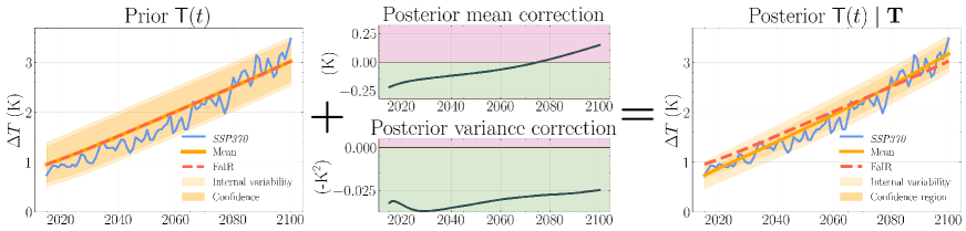
Figure 2: Emulation of NorESM2-LM SSP370 global mean surface temperature anomaly. Left: FaIRGP prior temperature response over SSP370. The prior mean response exactly corresponds to the FaIR temperature response, but with prior uncertainty quantification. Middle: Posterior correction for the mean and variance that learns from observation how to deviate from the prior. The pink area corresponds to deviations toward greater values and the green area deviations toward smaller values Right: FaIRGP posterior temperature response when updated with the other scenarios. The posterior response provides a sounder fit to observations, with better calibrated uncertainty.

5.2 Shared socio-economic pathways emulation

In this experiment, we consider the experiment dataset given by ${\mathcal{D}}=\{$historical, SSP126, SSP245, SSP370, SSP585$\}$. We iteratively remove one SSP experiment from the dataset to construct a training set (e.g. retain SSP245 to obtain ${\mathcal{D}}_{\text{train}}=\{$historical, SSP126, SSP370, SSP585$\}$) and use it to train FaIRGP and the baseline GP model. We run predictions over the retained SSP experiment and evaluate the emulated global temperatures against NorESM2-LM data. We find that on average, FaIRGP outperforms the baseline models in every evaluation metric, as reported in Table 4. These results suggest that FaIRGP provides a better emulation of the global temperature response to anthropogenic forcing compared to both FaIR and the plain GP model. We include in Appendix 8 a comparison with the GP emulator from ClimateBench [Watson-Parris . (2021)].

Table 4: Scores of baseline emulators and FaIRGP for the task of emulating SSPs global temperatures over 2015-2100 period ; the test experiment is retained from the training data and only used for evaluation ; the best emulator scores for each test experiment are highlighted in bold ; $\uparrow\!/\!\downarrow$ indicates higher/lower is better ; we report 1 standard deviation over the mean scores ; $\dagger$ indicates our proposed method.

Test experiment	Emulator	RMSE$\;\downarrow$	MAE$\;\downarrow$	Bias	LL$\;\uparrow$	Calib95	CRPS$\;\downarrow$
SSP126	FaIR	0.17	0.13	0.06	-	-	-
	Plain GP	0.18	0.14	0.08	0.23	1.0	0.10
	FaIRGP†	0.15	0.12	0.02	0.48	0.97	0.08
SSP245	FaIR	0.14	0.12	0.06	-	-	-
	Plain GP	0.09	0.07	0.03	0.67	1.0	0.06
	FaIRGP†	0.09	0.08	-0.01	0.71	1.0	0.06
SSP370	FaIR	0.22	0.19	0.10	-	-	-
	Plain GP	0.22	0.17	-0.16	0.12	1.0	0.12
	FaIRGP†	0.17	0.14	0.06	0.39	0.94	0.10
SSP585	FaIR	0.28	0.22	-0.07	-	-	-
	Plain GP	0.30	0.21	-0.12	0.16	1.0	0.14
	FaIRGP†	0.21	0.17	-0.08	0.18	0.88	0.12
Mean	FaIR	0.20$\pm$0.06	0.16$\pm$0.05	0.04$\pm$0.08	-	-	-
	Plain GP	0.20$\pm$0.09	0.15$\pm$0.06	-0.04$\pm$0.11	0.30$\pm$0.25	1.0$\pm$0.0	0.11$\pm$0.03
	FaIRGP†	0.16$\pm$0.05	0.12$\pm$0.04	-0.01$\pm$0.06	0.44$\pm$0.22	0.95$\pm$0.05	0.09$\pm$0.02

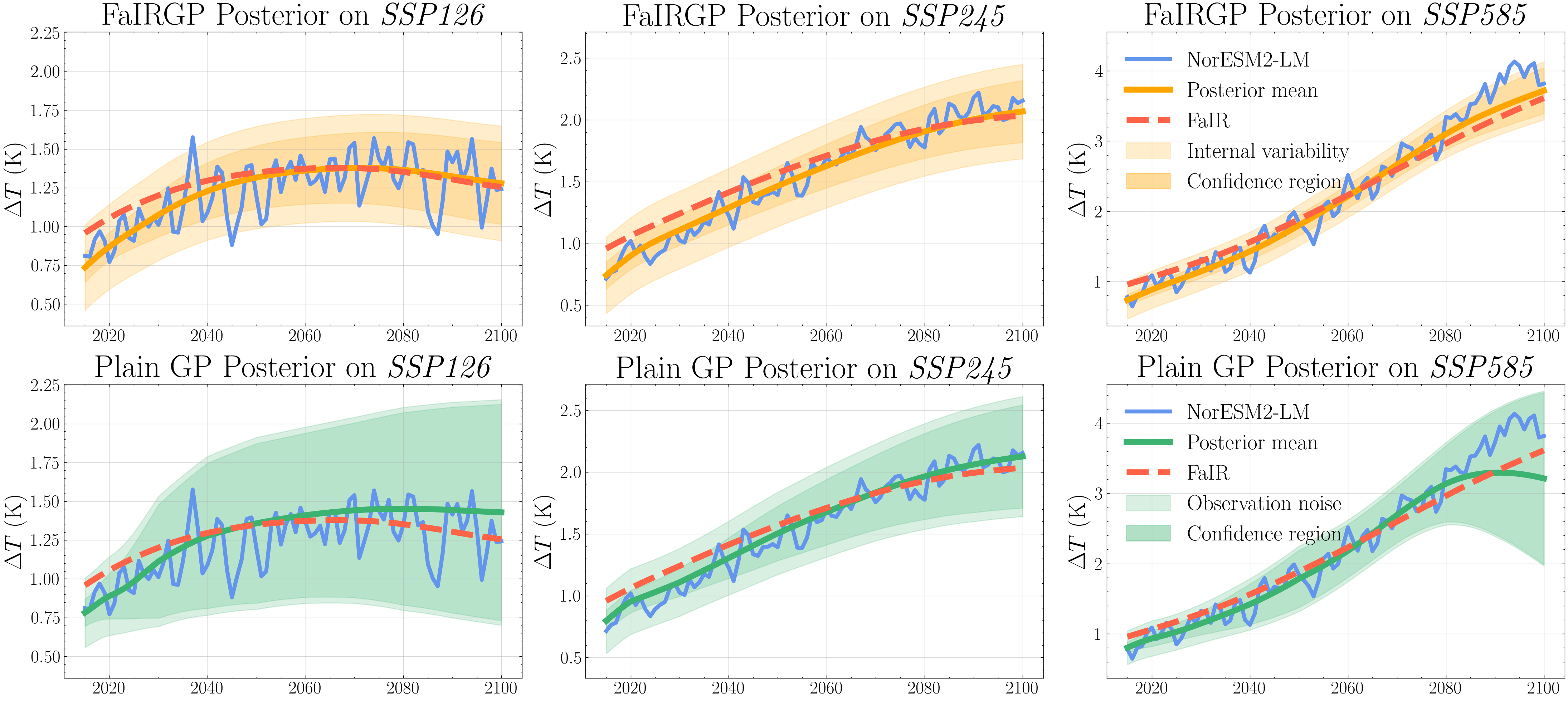
Figure 3: Emulated global mean surface temperature anomaly over 2015-2100 period with our FaIRGP emulator (top) and with a baseline GP emulator (bottom) for a low-forcing future scenario (SSP126), a medium forcing future scenario (SSP245) and a high forcing future scenario (SSP585).

Figure 3 shows that FaIRGP provides a better temperature projection than FaIR in the near future — over the 2015-2050 period — for all scenarios. This is because being informed by data grants FaIRGP the flexibility to deviate from the impulse response prior on which it hinges, and provide prediction that are better aligned with the historical and near future observations from the training set. However, when further away from the training data, over the 2080-2100 period, FaIRGP reverts back to the prior behavior of FaIR. This suggests that FaIRGP is better suited for emulating global temperature response in the near future, and at is least as good as FaIR for longer term emulation.

The plain GP model provides excellent predictions on SSP245, and even outperforms FaIRGP by a slight margin on deterministic metrics for this scenario. This is because GPs are notorious to excel at interpolation tasks, and the SSP245 scenario is a medium forcing scenario that perfectly lies within the range of the other low and high forcing scenarios used in the training data. However, when the evaluation scenario lies outside of the range of the training data, the plain GP model predictions will simply revert to the prior, and are therefore much less reliable. This is an important drawback of purely data-driven emulation, which by essence are interpolation models, and struggle to extrapolate outside the range of the training set. In Figure 3, this is particularly evident in the plain GP prediction on SSP585, where the model struggles at the end of the century due to unprecedented forcing levels that have not been seen in the training data. FaIRGP addresses this shortcoming by using FaIR as its prior, and therefore naturally reverts to an impulse response model when the prediction scenario is too distant from the training data.

Finally, FaIRGP provides a tighter and more robust uncertainty quantification over emulated temperatures compared to the plain GP model, which tends to overestimate the variance. This is reflected in Table 4 by a substantial improvement in LL of FaIRGP against the Plain GP, and suggests that the physics-informed covariance structure of FaIRGP is a sound choice to quantify emulator uncertainty. Further, the model formulated is able to quantify the uncertainty introduced by the internal variability separately from the uncertainty introduced by the emulator design. As shown in Figure 3, the uncertainty due to internal variability dominates in the near future, but the emulator uncertainty becomes predominant toward the end of the century, in accordance with the well-established assessment of hawkins2009potential.

5.3 Emulation from historical observations

In this experiment, we propose to investigate how well can the emulators generalise when they are solely trained on historical observations, and no simulated future data. We train the plain GP and FaIRGP using the historical experiment only, and evaluate predictions on all SSP scenarios. The results are reported in Table 5. We find that FaIRGP outperforms other models in almost every metric, and displays performance similar to FaIR only in mean bias.

Table 5: Scores of baseline emulators and FaIRGP when models are only trained using the historical experiment ; scores are evaluated and averaged for the task of emulating SSP126, SSP245, SSP370, SSP585 global surface temperatures over 2015-2100 period ; the best emulator for each metric is highlighted in bold ; $\uparrow\!/\!\downarrow$ indicates higher/lower is better ; $\dagger$ indicates our proposed method.

Emulator	RMSE$\;\downarrow$	MAE$\;\downarrow$	Bias	LL$\;\uparrow$	Calib95	CRPS$\;\downarrow$
FaIR	0.208	0.163	0.038	-	-	-
Plain GP	1.875	1.690	-1.690	-30.979	0.009	1.558
FaIRGP†	0.191	0.140	-0.037	0.314	0.948	0.102

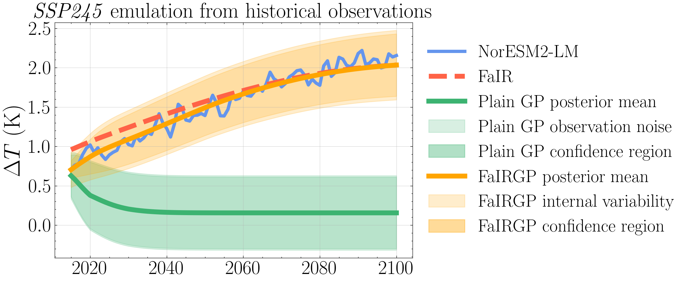
Figure 4: Emulated global mean surface temperature anomaly over 2015-2100 for the SSP245 scenario with emulators trained over historical temperatures only.

In this context a purely data-driven method struggles to extrapolate because it cannot marry the new previously unseen emission values with the underlying physical model. Figure 4 shows that the plain GP posterior immediately reverts to its prior after 2015, therefore providing uninformative temperature projections. On the other hand, FaIRGP manages to learn from historical observations to provide a better fit to the SSP over the 2015-2050 period, and slowly reverts back to the prior behavior of FaIR toward the end of the century.

This demonstrates the importance of having a robust underlying physical model to an emulator, and further suggests that FaIRGP is a well suited candidate for this task, and can provide meaningful temperature projections based only on historical observations.

5.4 Emulating radiative forcing from temperatures

In this experiment, we propose to evaluate how global surface temperature anomaly data can be used to inform an estimate of the effective radiative forcing using FaIRGP. We use the complete dataset of global temperature time series from the historical and SSP126, SSP245, SSP370, SSP585 experiments, which are depicted in Figure 5. We update the GP prior placed over the radiative forcing ${\mathsf{F}}(t)$ with temperature data to obtain a posterior radiative forcing response which incorporates information from temperature observations. We emphasise that the posterior over ${\mathsf{F}}(t)$ does not use any forcing observations, only temperature observations. As for temperature emulation, the posterior radiative forcing response is given in closed-form by (31). We evaluate the posterior historical radiative forcing response against NorESM2-LM historical top-of-atmosphere radiative forcing.

Figure 5 illustrates that the posterior forcing response learns from temperature time series how to deviate from the FaIR forcing trend to better account for observations. This is particularly evident between 1960 and 1980 where the posterior reproduces a decrease in forcing to better account for the global cooling trend in that time period, which FaIR struggles to capture. The results reported in Table 6 show that FaIRGP outperforms FaIR in RMSE and Bias at emulating historical global radiative forcing. Whilst FaIR performs better at emulating the stable forcing before 1950, FaIRGP better accounts for the forcing variations after 1950 and outperforms FaIR by a significant margin.

FaIRGP therefore proves to be useful to emulate global radiative forcing trends informed by surface temperatures. This is possible because our prior is specified within an energy balance model which explicitly connects the changes in surface temperatures to the changes in radiative forcing. On the contrary, this would not be possible with the plain GP model because it ignores forcing dynamics.

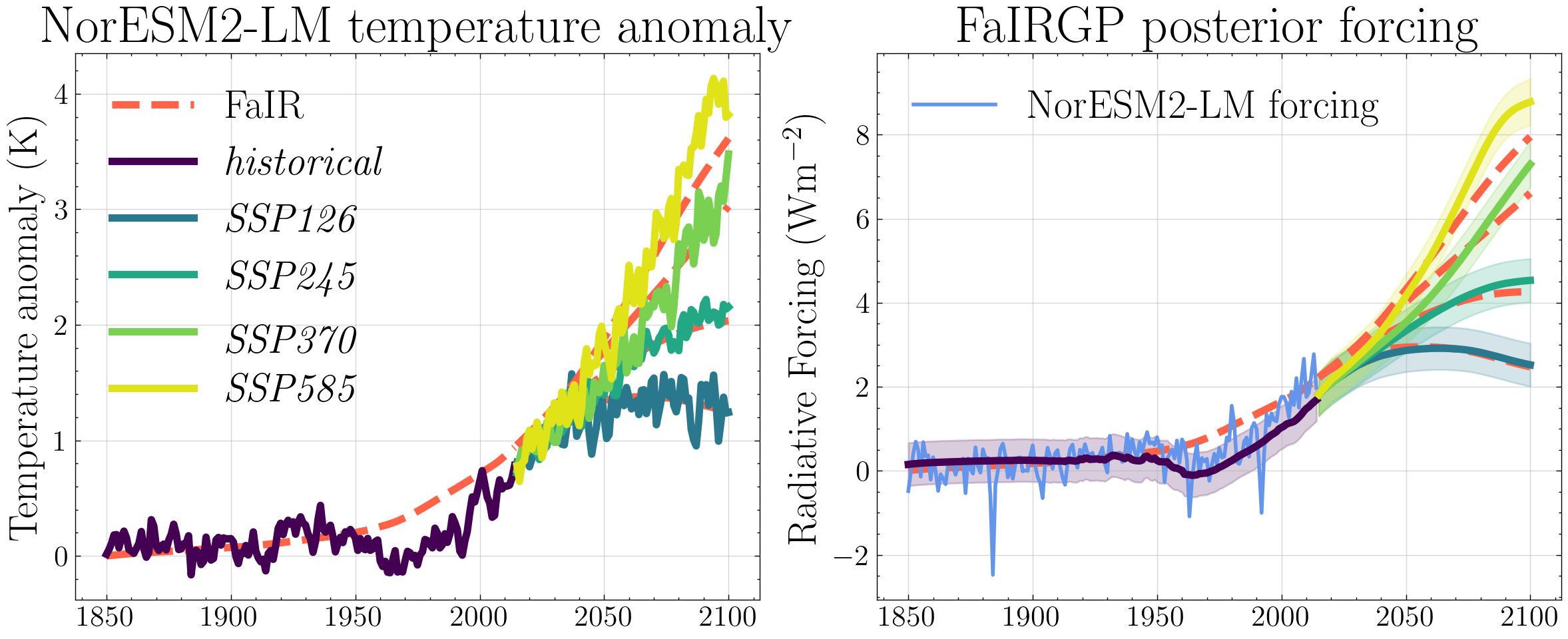
Figure 5: Left: Global temperature anomaly responses used to inform the posterior forcing response; Right: FaIRGP posterior radiative forcing predicted over experiments; the temperature response and radiative forcing obtained with FaIR are plotted in dashed red lines.

Table 6: Scores of FaIR and FaIRGP at emulating the global radiative forcing over historical periods ; scores are evaluated against NorESM2-LM top-of-atmosphere radiative forcing ; the best emulator scores for each period are highlighted in bold ; $\uparrow\!/\!\downarrow$ indicates higher/lower is better ; $\dagger$ indicates our proposed method.

Period	Emulator	RMSE$\;\downarrow$	MAE$\;\downarrow$	Bias	LL$\;\uparrow$	Calib95	CRPS$\;\downarrow$
1850-1950	FaIR	0.396	0.261	-0.008	-	-	-
	FaIRGP†	0.421	0.285	0.041	-0.585	0.99	0.216
1950-2014	FaIR	0.622	0.461	0.350	-	-	-
	FaIRGP†	0.568	0.466	-0.315	-0.865	0.938	0.321
1850-2014	FaIR	0.496	0.339	0.129	-	-	-
	FaIRGP†	0.484	0.357	-0.101	-0.695	0.970	0.257

6 Application: spatial surface temperatures emulation

In this section, we pursue the comparison of FaIRGP to baseline models, but for the task of emulating spatially-resolved temperatures. As for global emulation, we start by briefly illustrating how the model concretely applies. Then, we benchmark it against baseline models for SSP emulation and evaluate the emulation of surface temperatures forced by anthropogenic aerosols only. We conclude by investigating how FaIRGP can help emulate spatial top-of-atmosphere radiative forcing maps.

6.1 FaIRGP for spatial temperatures emulation

Figure 6 illustrates the spatial surface temperature anomaly emulation with FaIRGP for test scenario SSP245. As in the global case, a prior response based on FaIR is first specified, and then shifted by a data-informed posterior correction map. The posterior correction is learned from training scenarios ${\mathcal{D}}_{\text{train}}=\{$historical, SSP126, SSP370, SSP585$\}$.

The prior spatial response is constructed using a pattern scaling model trained on ${\mathcal{D}}_{\text{train}}$, and therefore introduces a fixed spatial pattern that is only rescaled by changes in global mean temperature. The posterior correction at location $x$ is obtained by updating the prior over ${\mathsf{T}}(x,t)$ from (33) with local surface temperature observations from ${\mathcal{D}}_{\text{train}}$. The posterior correction maps effectively provide a data-driven way to deviate from this fixed spatial pattern, and better account for the possibly varying spatial temperature patterns of the emulated scenario. Finally, by linearly adding the posterior correction map to the prior, we obtain a posterior spatial temperature response over SSP245.

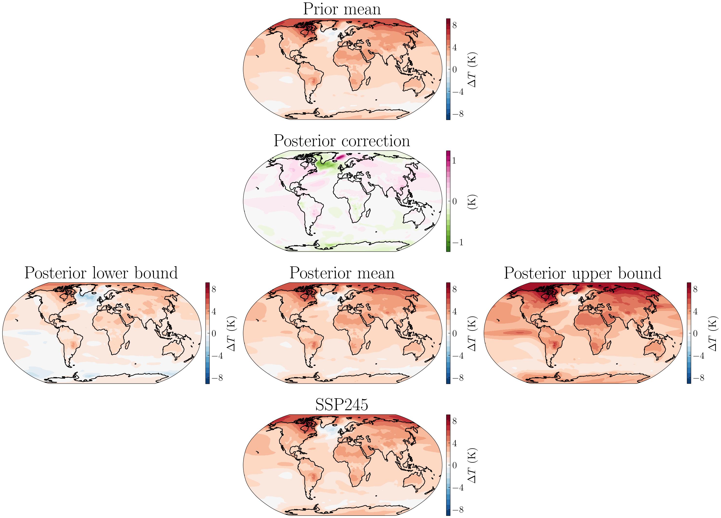
Figure 6: Spatial emulation of NorESM2-LM SSP245 temperatures. The prior mean (top) corresponds to a pattern scaling model used on FaIR global temperature response. The posterior correction (middle-top) learns from observations how to deviate from the pattern scaling prior to produce a posterior response (middle-bottom) that better emulates the groundtruth surface temperatures (bottom). The posterior lower/upper bound capture the 95% credible interval. Maps are averaged over 2080-2100 period.

Table 7: Scores of baseline emulators and FaIRGP for the task of emulating SSPs spatial temperatures over 2080-2100 period ; the best emulator for each metric is highlighted in bold ; $\uparrow\!/\!\downarrow$ indicates higher/lower is better ; we report 1 standard deviation ; $\dagger$ indicates our proposed method.

Emulator	RMSE$\;\downarrow$	MAE$\;\downarrow$	Bias	LL$\;\uparrow$	Calib95	CRPS$\;\downarrow$
Pattern scaling	0.637$\pm$0.189	0.467$\pm$0.139	-0.162$\pm$0.194	-	-	-
Plain GP	1.069$\pm$0.616	0.761$\pm$0.441	-0.362$\pm$0.350	-1.625$\pm$1.192	0.850$\pm$0.141	0.560$\pm$0.341
FaIRGP†	0.619$\pm$0.188	0.451$\pm$0.138	-0.113$\pm$0.192	-0.853$\pm$0.398	0.873$\pm$0.093	0.341$\pm$0.099

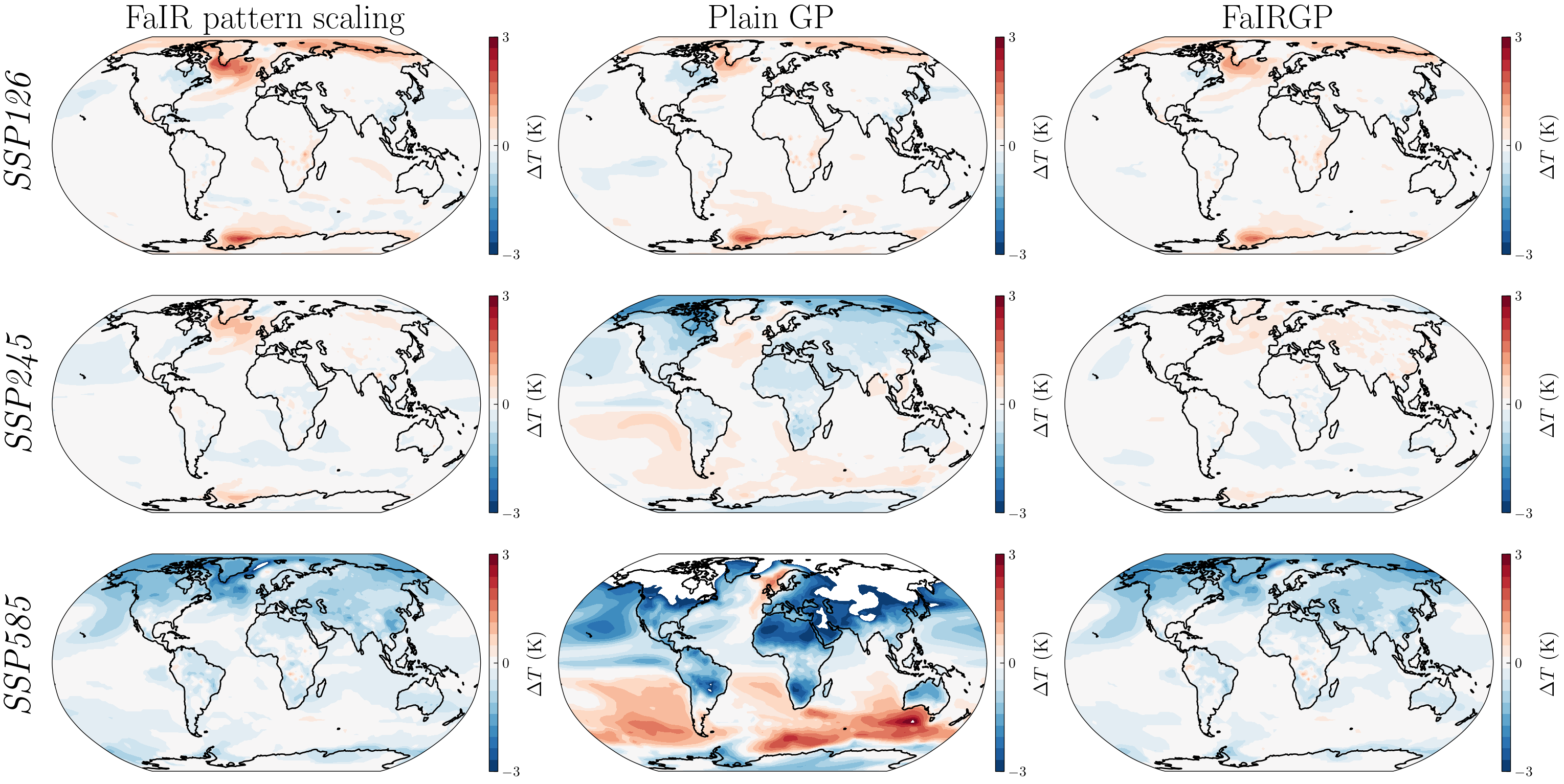
Figure 7: Maps of the mean difference between emulated spatial temperatures and target NorESM2 values for each emulator under a low forcing future scenario (SSP126), a medium forcing future scenario (SSP245) and a high forcing future scenario (SSP585). Red/Blue means the emulator overshoots/undershoots NorESM2 temperatures. Maps are averaged over the 2080-2100 period. Differences insignificant at the $p<0.05$ level are masked.

6.2 Shared socio-economic pathways emulation

In this experiment, we follow the same procedure as in the global emulation experiment and iteratively train models on the dataset deprived from one SSP scenario, then use the retained scenario as a test scenario for evaluation. We benchmark FaIRGP against a FaIR pattern scaling model and a purely data-driven plain GP emulator. The pattern scaling model is obtained by fitting a linear regression model using the same training data as the other models. The plain GP model is analogous to the baseline GP emulator in watsonparris2021climatebench, but differs in two aspects: (i) we adopt a simpler construction for the covariance with a Matérn-3/2 kernel with automatic relevance determination, and (ii) our model takes as input global aerosols emissions whereas watsonparris2021climatebench use spatially-resolved aerosols emission maps. Scores are computed over the 2080-2100 period since the start of all SSPs is quite similar. Mean scores are reported in Table 7.

We find that FaIRGP has on average lower error than baseline models. Figure 7 shows that the spatial bias patterns of FaIRGP are similar to the bias patterns obtained with the FaIR pattern scaling model. This indicates that the prior has a strong influence on the predicted posterior. Nonetheless, we observe that the posterior correction in FaIRGP helps mitigate the spatial inaccuracies of its prior. This is particularly evident for SSP126 and SSP245 where the magnitude of the spatial bias in FaIRGP is overall smaller than the one for the FaIR pattern scaling model. Regarding the high forcing scenario SSP585, the spatial correction is more subtle. This is due to it becoming an extrapolation task, and as a result, FaIRGP exhibits behavior closer to its pattern scaling prior.

Figure 7 also shows that, as for global temperature emulation, the plain GP model predicts sound surface temperature maps for low and medium forcing scenarios, but struggles at extrapolating over high forcing scenarios.

6.3 Emulating anthropogenic aerosols forcing

In this experiment, we want to evaluate emulation of temperature changes induced by anthropogenic aerosols emissions. We use the hist-aer experiment from the ClimateBench v1.0 dataset. The hist-aer experiment is generated using NorESM2-LM, using only historical anthropogenic aerosols emissions, and setting long-lived greenhouse gases emissions to zero. We emulate surface temperatures over this scenario using emulators trained on all available historical and SSPs experiments.

Figure 8 illustrates the challenges faced by the baseline pattern scaling model in reproducing the magnitude and spatial patterns of the temperature cooling effect induced by aerosols. The introduction of a correction through FaIRGP improves the overall magnitude of the cooling effect. The predicted spatial temperature pattern with FaIRGP remains nonetheless strongly influenced by the prior spatial pattern.

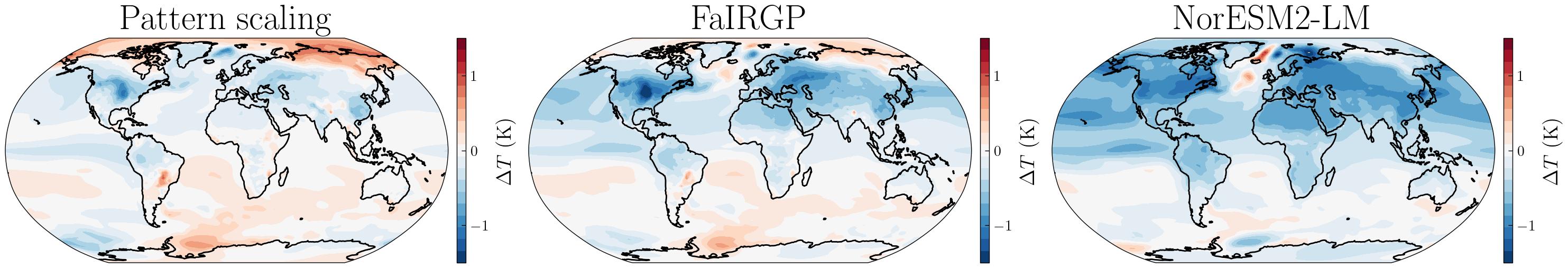
Figure 8: Maps of surface temperatures averaged for the hist-aer experiment averaged over 1900-2014 period. Left: Prediction with the FaIR pattern scaling baseline. Middle: Prediction with the FaIRGP posterior mean. Right: Groundtruth NorESM2-LM surface temperatures map.

This shows that FaIRGP clearly improves over the pattern scaling baseline at emulating the temperature changes resulting from anthropogenic aerosols emissions. This task is notoriously difficult for pattern scaling models, which excel at emulating responses to greenhouse gas emissions but struggle under strong aerosol forcing scenarios [May (2012), Levy . (2013)]. Considering the significant impact of the prior choice on FaIRGP, this fosters advocacy for a prior local response model that goes beyond pattern scaling models. Finally, whilst we only use global aerosols emissions, using spatially-resolved emissions maps should improve emulated temperatures given the strong influence spatial patterns of aerosols have over radiative forcing [Williams . (2022)].

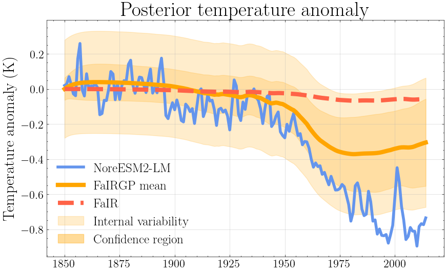
Figure 10: Emulated global mean surface temperature anomaly over 1850-2014 for the hist-aer scenario with FaIRGP trained over historical, SSP126, SSP245, SSP370, SSP585.

In addition we note that, for parameters calibrated against NorESM2-LM, FaIR exhibits difficulties in capturing the aerosol forcing, as illustrated in Figure 10. This limitation is likely to affect the performance of the pattern scaling model.

B provides emulation results with a plain GP model. As anticipated, the purely data-driven emulator faces difficulties in emulating surface temperatures solely based on aerosols emissions inputs, primarily because every scenario from its training data includes greenhouse gas emissions.

6.4 Emulating radiative forcing from temperatures

As in Section 5.4, we propose to probe whether FaIRGP can be used to estimate spatial forcing maps. Since we do not have a spatial forcing model, we simply use a spatially constant forcing prior for ${\mathsf{F}}(x,t)$. We update it with spatially-resolved temperature observations from historical and SSPs scenarios. Figure 9 compares the obtained posterior mean forcing with historical forcing maps simulated with NorESM2-LM.

The magnitude of the emulated posterior forcing is relatively conservative and does not reach the same level as the ground truth maps. However, the emulated forcing successfully captures the hemispheric contrast during the 1960-1990 period, as well as the overall temporal increase and large-scale spatial forcing patterns. Despite struggling to reproduce the same magnitude of the forcing, this is encouraging considering that the emulated spatial patterns are solely inferred from temperature patterns. Using a more informative prior for the spatial forcing could easily help improve these results.

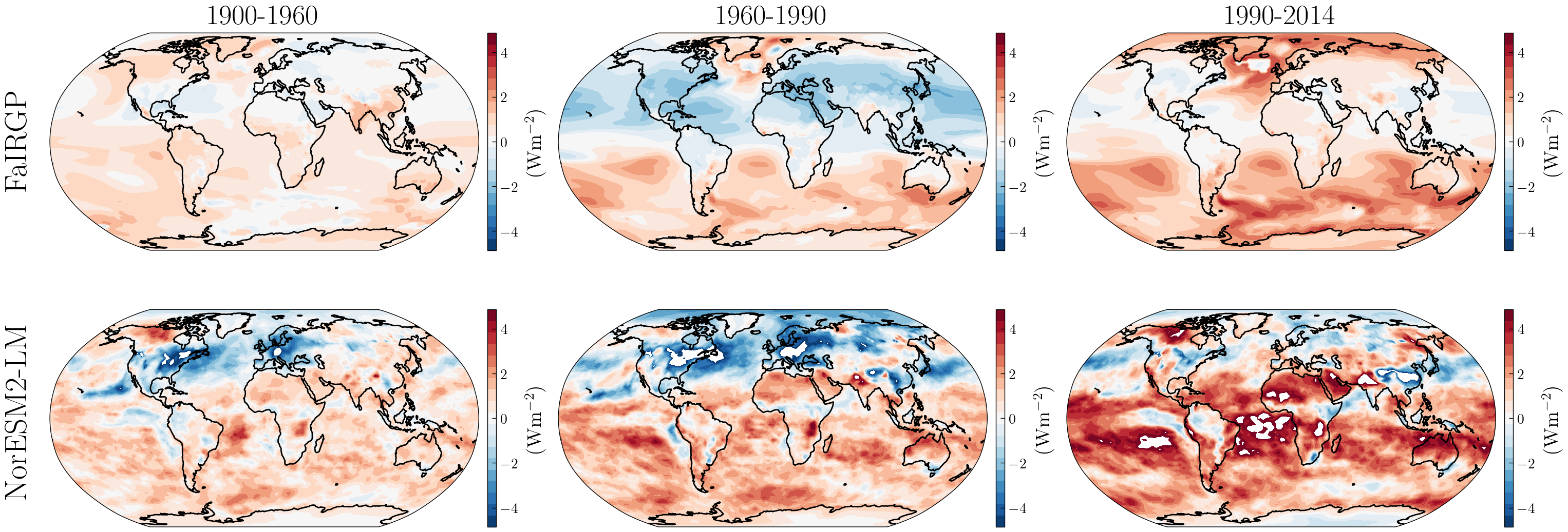
Figure 9: Maps of top-of-atmosphere radiative forcing averaged over 1900-1960, 1960-1990 and 1990-2014 periods of the historical scenario. Top: Mean posterior radiative forcing predicted with FaIRGP. Bottom: NorESM2-LM radiative forcing maps.

7 Discussion

7.1 About the GP approach

7.1.1 Comparison to placing Bayesian priors over the SCM parameters

A simple way to introduce model variability in simple climate models is to place Bayesian priors over model parameters, such as the carbon cycle feedback terms or the forcing model coefficients [Leach . (2021)]. Such priors can then be updated with global temperatures observations to formulate posterior distributions. This specifies a probabilistic climate model calibrated against observations. Whilst aligned in spirit with the work proposed in this paper, we argue that our GP-based approach displays several advantages over placing priors on model parameters.

Chiefly, FaIRGP formulates analytical expressions for the posterior distribution over forcing and temperatures, which have an intuitive interpretation as the sum of a physics-driven prior and a data-driven correction. In contrast, when placing a Bayesian prior over parameters, we do not in general have access to a probability distribution for temperatures. Therefore, probabilistic emulation may need to be sampling based, and one must resort to more complex Markov-Chain Monte-Carlo (MCMC) techniques to sample from the posterior distribution.

Sampling-based approaches have two main shortcomings: (i) a thorough uncertainty quantification requires storing a tremendous amount of scenarios, which can be limited by memory capacity — beusch2022emission require an ensemble of 9 millions emulations; (ii) it reduces the statistical representation of uncertainty to summary statistics such as the mean, standard deviation or quantiles. In contrast, having a closed-form expression for the posterior distribution with GPs allows to analytically conduct probabilistic studies using the full probability density, and additionally draw samples, if needed.

Finally, having access to the probability density expression allows to evaluate the likelihoods of observations. This can critically be used as a maximisation objective to tune the model parameters against observations, but also in the context of Bayesian optimisation routines to find optimal emission trajectories to meet climate goals.

7.1.2 Connection with stochastic energy balance models

Our work is related to the work of cummins2020optimal, which formulates a stochastic energy balance model by introducing a white noise variability term in the temperature response and the forcing models. This allows them to account for climate internal variability, and formulate a Kalman filtering strategy to obtain maximum likelihood estimators of the energy balance model parameters. Our work similarly introduces a white noise in the temperature response model to account for climate internal variability, which results in an additional temporal Matérn-1/2 covariance term in the prior over temperatures. Whilst an extended discussion goes beyond the scope of this work, it can be shown that in the long term regime, these two approaches are equivalent, and that more broadly, Kalman filtering models are in fact equivalent to temporal GPs with Matérn covariance functions [Hartikainen  Särkkä (2010), Sarkka  Hartikainen (2012), Sarkka . (2013)].

Our work differs from cummins2020optimal in that beyond the stochasticity arising from internal variability, we also introduce a GP prior over the radiative forcing. This GP prior introduces stochasticity over the SCM design, which is not only a function of time, but also of emission levels. Because our modelling is not purely temporal (the GP is also a function of emissions), we cannot employ Kalman filtering strategies and instead choose to use GP regression techniques.

7.1.3 Choice of kernel $\rho$

The choice of covariance function $\rho$ in (12) is an important choice that allows the user to incorporate their domain knowledge into the prior over the radiative forcing. Let $u$ and $u^{\prime}$ be generic notations for input data (in our work, greenhouse gas and aerosols emissions), the kernel $\rho(u,u^{\prime})$ specifies how will the prior covary between these two inputs. For example, choosing $\rho(u,u^{\prime})=\delta(u-u^{\prime})$ makes the GP independent at any two inputs. On the other hand, choosing $\rho(u,u^{\prime})=1$ causes the GP to covary equally between any two inputs.

The Matérn family are a common family of kernel parameterised by a degree $\nu$. They allow to control for the functional regularity of the GP. For $\nu=1/2$, draws from the GP are continous functions, for $\nu=3/2$ they are once differentiable, and in the limit $\nu=\infty$ they become infinitely differentiable. A detailed presentation of the Matérn kernels is provided in Appendix C.2.

Additions or multiplications of kernels can be used to construct more elaborate covariance functions that reflect an additive or multiplicative structure in the forcing. Periodic kernels can also be introduced to model seasonality. Going further, more complex choices of kernels include the spectral mixture kernel [A. Wilson  Adams (2013)] which attemps to learn the spectral density of the data, or even kernels parametrised as neural networks [AG. Wilson . (2016), Law . (2019)].

Whilst kernel selection plays a key role in GP regression, our focus in this work is on the development of the FaIRGP framework rather than refining the kernel itself. The kernel is treated throughout as a modular component, with potential for refinement. As a result, we choose to work with a simple Matérn-3/2 kernel with automatic relevance determination throughout. Preliminary findings indicate that the choice of kernel does not significantly degrade the results. Hence, dedicating efforts to constructing more elaborate kernels is likely to yield comparable or better results than our current approach.

7.1.4 Computational efficiency and scalability

We report that to emulate 100 years of surface temperature anomaly with FaIRGP, it takes less than a second for global and spatial emulation on an “average” personal laptop, without requiring any parallelization methods.

Scalability issues are commonly associated with Gaussian Processes (GPs) when the training set grows in size. This is because computing their posterior distribution involves a matrix inversion, which has a cubic computational cost in the number of training samples. Fortunately, unlike neural networks which require large amounts of data [Watson-Parris . (2021)], GPs excel in scenarios with limited data [Rasmussen  Williams (2005)]. Consequently, it is possible to develop skilful GP emulators with limited training data.

In cases where using a larger training dataset becomes a necessity, one can still employ linear conjugate gradients methods and parallelisation schemes [Wang . (2019)] to scale exact GPs to millions of data points. Alternatively, sparse approximation techniques can be used to obtain a scalable estimate of the posterior distribution [Rahimi  Recht (2007), Titsias (2009), Matthews . (2016)].

7.2 Climate modelling considerations

7.2.1 Beyond FaIR: broader applicability of the method

While we have chosen to use FaIR as the backbone climate model for our work, the rationale behind the development of FaIRGP is easily transferable to other commonly used simple climate models such as MAGICC [Meinshausen . (2011)] or OSCAR [Gasser . (2017)]. These models share linear time invariant dynamics, allowing us to incorporate a GP prior into the forcing term of these dynamics. By doing so, we can obtain a GP-based solution that is informed the model parameters, exactly like in FaIRGP.

The dynamical systems of interest can naturally describe the temperature response to radiative forcing, as it is the case in our work. However, we could also imagine extending this to carbon cycle models, where emission levels prescribe the forcing function, and the output of the dynamical system are atmospheric concentrations. This GP framework over dynamical systems is in fact highly general, and has been introduced by alvarez2009latent in the context of dynamical systems where the forcing function is unknown.

7.2.2 Pixel independence assumption

The pattern scaling model used in our prior effectively uses independent linear regressions at each location to map changes in global mean temperature onto changes in local temperature. However, this modeling approach challenges our intuition as it overlooks the spatial dependence of temperature fields, despite our expectation that temperatures at nearby locations should covary.

To address this modeling concern, a common solution is to incorporate spatially correlated innovations into the pattern scaling response, which represent the spatial expression of climate internal variability [Beusch . (20202), Beusch . (20201), Beusch . (2022), Castruccio  Stein (2013), Goodwin . (2020)]. Alternatively, link2019fldgen design a procedure based on the Wiener-Khinchin theorem [Champeney  Fuoss (1973)] to emulate a climate variability field with the same variance and spatiotemporal correlation structure as the one in ESMs outputs.

From a statistical modeling standpoint, these approaches introduce spatial variability as multivariate Gaussian variables, differing only in their covariance structure. Consequently, they can be easily incorporated into our GP framework. However, for the sake of clarity, we chose not to delve into these additional considerations and instead focus on the exposition of the Bayesian energy balance model.

Further, whilst it has been pointed out that, in general, regional changes in temperature scale robustly with global temperature [Seneviratne . (2016)], this may not be true under strong mitigation scenarios or under strong aerosol forcing [May (2012), Levy . (2013)]. This fosters advocacy for development of “spatialised” simple climate models going beyond pattern scaling.

7.2.3 Opportunities for precipitation emulation

Going beyond surface temperature emulation, we can explore how FaIRGP can be used to emulate precipitations. One approach is to combine the Gaussian process GP emulator for precipitation described in watsonparris2021climatebench with FaIRGP. By leveraging Gaussian conjugacy relationships, a natural cross-covariance between the two emulators is induced. This enables the exchange of information between precipitation and temperature fields. This is in line with recent advocacy for joint emulation of temperatures and precipitations [Snyder . (2019), Schöngart . (2022), Schöngart . (2023)].

Another option is to use the emulated temperatures from FaIRGP as input for a statistical emulator of precipitation, such as a Gamma regression model [Martinez-Villalobos  Neelin (2019)]. Indeed, many climate impacts are routinely assumed to be a function of temperatures. Additionally, the full probability distribution predicted by FaIRGP can be incorporated into the model, allowing for the propagation of epistemic uncertainty associated with FaIRGP.

7.2.4 Application to detection and attribution

With FaIRGP, we have access to the analytical expression of the probability density distribution of emulated temperatures. Therefore, we can emulate surface temperatures under historical scenarios, both with and without anthropogenic forcing, and analytically compute the probability of temperature occurrences in each scenario. By comparing these probabilities, we can assess the extent to which human activity has made a certain temperature range more likely, enabling us to conduct attribution studies.

Conducting detection and attribution studies with emulators is not exclusive to FaIRGP, and could in principle be conducted with any emulator as discussed in watsonparris2021climatebench. However, the strength of FaIRGP lies in its ability to input temperature ranges directly into a known probability density function, providing a precise probability between 0 and 1 of such temperatures to occur under a given emission scenario.

8 Conclusion and outlooks

Simple climate models (SCMs) are robust physically-motivated emulators of changes in global mean surface temperatures. Gaussian processes (GPs) are powerful Bayesian machine learning model capable of learning complex relationships, and emulate from data how changes in emissions affect changes in surface temperatures. By combining them together, we reconcile these two paradigms of emulator design, which mutually address their respective limitations. We introduce FaIRGP, a Bayesian energy balance model that (i) maintains the robustness and interpretability of a simple climate model, (ii) gains the flexibility of modern statistical machine learning models with the ability to learn from data, and (iii) provides principled uncertainty quantification over the emulator design.

We demonstrate skilful emulation of global mean surface temperatures over realistic emission scenarios. Unlike GPs, FaIRGP has a robust physical grounding which allows it to provide reliable predictions even on out-of-sample scenarios. On the other hand, unlike SCMs, FaIRGP can learn complex non-linear relationships to deviate from an SCM and improve predictions. In particular, FaIRGP better accounts for the temperature response to anthropogenic aerosols emissions. We further show that these findings carry over for the task of emulating spatially-resolved surface temperature maps. In addition, we find that FaIRGP can also be used to produce estimates of top-of-atmosphere radiative forcing given temperature observations.

The full mathematical tractability, with analytical expressions for probability distributions, provides great control over the modelling, and a rich framework to reason about probability distributions over temperatures. This is of great relevance to detection and attribution studies. Further, whilst our work focuses on temperature emulation — which have already been thoroughly studied — we envision FaIRGP as a foundation for the development of robust data-driven emulators for more complex climate variables, such as precipitations. Harnessing the mathematical properties of GPs, we believe that emulating climate impacts using FaIRGP will provide additional control over pure machine learning methods, whilst being able to capture complex non-linear relationships to forcing.

We hope this work will contribute to building trust in data-driven models, and thereby allow the climate science community to benefit more widely from their potential.

Appendix A Supporting materials for FaIRGP derivation

A.1 Useful results

Lemma A.1.

Let $a,b>0$ and $u,v\geq 0$. We have

$$(a+b)\min(u,v)-(au+bv)=\begin{cases}-b|u-v|&\text{if }u\leq v\\ -a|u-v|&\text{if }u\geq v.\end{cases}$$ (35)

Proof.

If $u\leq v$,

$$(a+b)\min(u,v)-(au+bv) =(a+b)u-au-bv$$

$$=bu-bv$$

$$=-b|u-v|.$$

If $u\geq v$,

$$(a+b)\min(u,v)-(au+bv) =(a+b)v-au-bv$$

$$=av-au$$

$$=-a|u-v|.$$

∎

A.2 Derivation of FaIRGP

Consider a $k$-box EBM specified by the stochastic temperature response model

$$\,{\mathrm{d}}\boldsymbol{\mathsf{X}}(t)={\mathbf{A}}\boldsymbol{\mathsf{X}}(t)\,{\mathrm{d}}t+{\mathbf{b}}{\mathsf{F}}(t)\,{\mathrm{d}}t,$$ (36)

where ${\mathsf{F}}(t)\sim{\operatorname{GP}}(F,K)$, a forcing feedback vector ${\mathbf{b}}=\begin{bmatrix}1/C_{1}&0&\ldots&0\end{bmatrix}^{\top}$, and a forcing feedback matrix given by

Denote ${\mathbf{A}}={\boldsymbol{\Phi}}{\mathbf{D}}{\boldsymbol{\Phi}}^{-1}$ the diagonalisation of the feedback matrix, where ${\mathbf{D}}$ is a diagonal matrix with diagonal elements

$${\mathbf{D}}=\operatorname{Diag}(D_{1},\ldots,D_{k}).$$ (37)

Then we have

$$\,{\mathrm{d}}\boldsymbol{\mathsf{X}}(t)={\mathbf{A}}\boldsymbol{\mathsf{X}}(t)\,{\mathrm{d}}t+{\mathbf{b}}{\mathsf{F}}(t)\,{\mathrm{d}}t$$ (38)

$$\Rightarrow {\boldsymbol{\Phi}}^{-1}\,{\mathrm{d}}\boldsymbol{\mathsf{X}}(t)={\mathbf{D}}{\boldsymbol{\Phi}}^{-1}\boldsymbol{\mathsf{X}}(t)\,{\mathrm{d}}t+{\boldsymbol{\Phi}}^{-1}{\mathbf{b}}{\mathsf{F}}(t)\,{\mathrm{d}}t$$ (39)

$$\Rightarrow \,{\mathrm{d}}\left[{\boldsymbol{\Phi}}^{-1}\boldsymbol{\mathsf{X}}(t)\right]={\mathbf{D}}\left[{\boldsymbol{\Phi}}^{-1}\boldsymbol{\mathsf{X}}(t)\right]\,{\mathrm{d}}t+\left[{\boldsymbol{\Phi}}^{-1}{\mathbf{b}}\right]{\mathsf{F}}(t)\,{\mathrm{d}}t.$$ (40)

Therefore, by using the notations from [Millar . (2017)]

$$D_{i} =-1/d_{i}$$ (41)

$${\boldsymbol{\Phi}}^{-1}\boldsymbol{\mathsf{X}}(t) =\begin{bmatrix}{\mathsf{S}}_{1}(t)&\ldots&{\mathsf{S}}_{k}(t)\end{bmatrix}^{\top}$$ (42)

$${\boldsymbol{\Phi}}^{-1}{\mathbf{b}} =\begin{bmatrix}q_{1}/d_{1}&\ldots&q_{k}/d_{k}\end{bmatrix}^{\top},$$ (43)

the diagonalised system can be written as an impulse response system, where for $i\in\{1,\ldots,k\}$ we have

$$\boxed{\,{\mathrm{d}}{\mathsf{S}}_{i}(t)=-\frac{1}{d_{i}}{\mathsf{S}}_{i}(t)\,{\mathrm{d}}t+\frac{q_{i}}{d_{i}}{\mathsf{F}}(t)\,{\mathrm{d}}t=\frac{1}{d_{i}}(q_{i}{\mathsf{F}}(t)-{\mathsf{S}}_{i}(t))\,{\mathrm{d}}t.}$$ (44)

Consider now the thermal response ${\mathsf{S}}_{i}(t)$ of the $i$^th SDE. This thermal response is given by

$${\mathsf{S}}_{i}(t)=\frac{q_{i}}{d_{i}}\int_{0}^{t}{\mathsf{F}}(s)e^{-(t-s)/d_{i}}\,{\mathrm{d}}s,$$ (45)

where we recall that ${\mathsf{F}}(t)\sim{\operatorname{GP}}(F,K)$. Because GPs are closed under linear transformations, ${\mathsf{S}}_{i}(t)$ must also be GPs for all $i\in\{1,\ldots,k\}$. Their mean functions can be computed following

$$m_{i}(t):={\mathbb{E}}[{\mathsf{S}}_{i}(t)] ={\mathbb{E}}\left[\frac{q_{i}}{d_{i}}\int_{0}^{t}{\mathsf{F}}(s)e^{-(t-s)/d_{i}}\,{\mathrm{d}}s\right]$$ (46)

$$=\frac{q_{i}}{d_{i}}\int_{0}^{t}{\mathbb{E}}[{\mathsf{F}}(s)]e^{-(t-s)/d_{i}}\,{\mathrm{d}}s$$ (47)

$$=\frac{q_{i}}{d_{i}}\int_{0}^{t}F(s)e^{-(t-s)/d_{i}}\,{\mathrm{d}}s.$$ (48)

Their cross-covariance functions can be computed following

$$k_{ij}(t,t^{\prime}) :=\operatorname{Cov}({\mathsf{S}}_{i}(t),{\mathsf{S}}_{j}(t^{\prime}))$$ (49)

$$=\operatorname{Cov}\left(\frac{q_{i}}{d_{i}}\int_{0}^{t}{\mathsf{F}}(s)e^{-(t-s)/d_{i}}\,{\mathrm{d}}s,\frac{q_{j}}{d_{j}}\int_{0}^{t^{\prime}}{\mathsf{F}}(s^{\prime})e^{-(t^{\prime}-s^{\prime})/d_{j}}\,{\mathrm{d}}s^{\prime}\right)$$ (50)

$$=\frac{q_{i}q_{j}}{d_{i}d_{j}}\int_{0}^{t}\int_{0}^{t^{\prime}}\operatorname{Cov}({\mathsf{F}}(s),{\mathsf{F}}(s^{\prime}))e^{-(t-s)/d_{i}}e^{-(t^{\prime}-s^{\prime})/d_{j}}\,{\mathrm{d}}s\,{\mathrm{d}}s^{\prime}$$ (51)

$$=\frac{q_{i}q_{j}}{d_{i}d_{j}}\int_{0}^{t}\int_{0}^{t^{\prime}}K(s,s^{\prime})e^{-(t-s)/d_{i}}e^{-(t^{\prime}-s^{\prime})/d_{j}}\,{\mathrm{d}}s\,{\mathrm{d}}s^{\prime}.$$ (52)

So we have ${\mathsf{S}}_{i}(t)\sim{\operatorname{GP}}(m_{i},k_{ii})$ for any $i\in\{1,\ldots,k\}$. Finally, if we define ${\mathsf{T}}(t)=\sum_{i=1}^{k}{\mathsf{S}}_{i}(t)$, since the sum of Gaussians is still a Gaussian, we know that ${\mathsf{T}}(t)$ must also be a GP. And we can compute its mean function following

$$m_{\mathsf{T}}(t):={\mathbb{E}}[{\mathsf{T}}(t)]={\mathbb{E}}\left[\sum_{i=1}^{k}{\mathsf{S}}_{i}(t)\right]=\sum_{i=1}^{k}{\mathbb{E}}[{\mathsf{S}}_{i}(t)]=\sum_{i=1}^{k}m_{i}(t),$$ (54)

and its covariance function following

$$k_{\mathsf{T}}(t,t^{\prime}):=\operatorname{Cov}({\mathsf{T}}(t),{\mathsf{T}}(t^{\prime})) =\operatorname{Cov}\left(\sum_{i=1}^{k}{\mathsf{S}}_{i}(t),\sum_{j=1}^{k}{\mathsf{S}}_{j}(t^{\prime})\right)$$ (55)

$$=\sum_{i=1}^{k}\sum_{j=1}^{k}\operatorname{Cov}({\mathsf{S}}_{i}(t),{\mathsf{S}}_{j}(t^{\prime}))$$ (56)

$$=\sum_{i=1}^{k}\sum_{j=1}^{k}k_{ij}(t,t^{\prime}).$$ (57)

We conclude that

$$\boxed{\left\{\begin{aligned} \hfil\displaystyle\begin{split}&{\mathsf{T}}(t)\sim{\operatorname{GP}}(m_{\mathsf{T}},k_{\mathsf{T}})\\ &m_{\mathsf{T}}(t)=\sum_{i=1}^{k}m_{i}(t)\\ &k_{\mathsf{T}}(t,t^{\prime})=\sum_{i=1}^{k}\sum_{j=1}^{k}k_{ij}(t,t^{\prime}).\end{split}\end{aligned}\right.}$$ (58)

A.3 Accounting for climate internal variability in FaIRGP

Consider again the same problem, but introducing an additional white noise term in the temperature response SDE

$$\,{\mathrm{d}}\boldsymbol{\mathsf{X}}(t)={\mathbf{A}}\boldsymbol{\mathsf{X}}(t)\,{\mathrm{d}}t+{\mathbf{b}}{\mathsf{F}}(t)\,{\mathrm{d}}t+\sigma{\mathbf{b}}\,{\mathrm{d}}{\mathsf{B}}(t),$$ (59)

where ${\mathsf{B}}(t)$ denotes the standard Brownian motion.

Following the same derivation steps we get

$$\,{\mathrm{d}}\boldsymbol{\mathsf{X}}(t)={\mathbf{A}}\boldsymbol{\mathsf{X}}(t)\,{\mathrm{d}}t+{\mathbf{b}}{\mathsf{F}}(t)\,{\mathrm{d}}t+\sigma{\mathbf{b}}\,{\mathrm{d}}{\mathsf{B}}(t)$$ (60)

$$\Rightarrow {\boldsymbol{\Phi}}^{-1}\,{\mathrm{d}}\boldsymbol{\mathsf{X}}(t)={\mathbf{D}}{\boldsymbol{\Phi}}^{-1}\boldsymbol{\mathsf{X}}(t)\,{\mathrm{d}}t+{\boldsymbol{\Phi}}^{-1}{\mathbf{b}}F(t)\,{\mathrm{d}}t+{\boldsymbol{\Phi}}^{-1}{\mathbf{c}}\,{\mathrm{d}}{\mathsf{B}}(t)$$ (61)

$$\Rightarrow \,{\mathrm{d}}\left[{\boldsymbol{\Phi}}^{-1}\boldsymbol{\mathsf{X}}(t)\right]={\mathbf{D}}\left[{\boldsymbol{\Phi}}^{-1}\boldsymbol{\mathsf{X}}(t)\right]\,{\mathrm{d}}t+\left[{\boldsymbol{\Phi}}^{-1}{\mathbf{b}}\right]{\mathsf{F}}(t)\,{\mathrm{d}}t+\sigma\left[{\boldsymbol{\Phi}}^{-1}{\mathbf{b}}\right]\,{\mathrm{d}}{\mathsf{B}}(t).$$ (62)

which gives in impulse response form

$$\boxed{\,{\mathrm{d}}{\mathsf{S}}_{i}(t)=\frac{1}{d_{i}}(q_{i}{\mathsf{F}}(t)-{\mathsf{S}}_{i}(t))\,{\mathrm{d}}t+\sigma\frac{q_{i}}{d_{i}}\,{\mathrm{d}}{\mathsf{B}}(t),\enspace\forall i\in\{1,\ldots,k\}.}$$ (63)

The solution to the $i$^th SDE is now given by

$${\mathsf{S}}_{i}(t) =\underbrace{\frac{q_{i}}{d_{i}}\int_{0}^{t}{\mathsf{F}}(s)e^{-(t-s)/d_{i}}\,{\mathrm{d}}s}_{{\mathsf{S}}_{i}^{\circ}(t)}+\sigma\underbrace{\frac{q_{i}}{d_{i}}\int_{0}^{t}e^{-(t-s)/d_{i}}\,{\mathrm{d}}{\mathsf{B}}(s)}_{\eta_{i}(t)}$$ (64)

$$={\mathsf{S}}_{i}^{\circ}(t)+\sigma\eta_{i}(t).$$ (65)

${\mathsf{S}}_{i}^{\circ}(t)$ corresponds to the GP we have obtained in the previous derivation without white noise, i.e. ${\mathsf{S}}_{i}^{\circ}(t)\sim{\operatorname{GP}}(m_{i},k_{ii})$. $\eta_{i}(t)$ is also a GP, with mean zero, and cross-covariance function given by

$$\operatorname{Cov}(\eta_{i}(t),\eta_{j}(t^{\prime})) ={\mathbb{E}}\left[\left(\eta_{i}(t)-{\mathbb{E}}[\eta_{i}(t)]\right)\left(\eta_{j}(t^{\prime})-{\mathbb{E}}[\eta_{j}(t^{\prime})]\right)\right]$$

$$={\mathbb{E}}[\eta_{i}(t)\eta_{j}(t^{\prime})]$$

$$={\mathbb{E}}\left[\left(\frac{q_{i}}{d_{i}}\int_{0}^{t}e^{-(t-s)/d_{i}}\,{\mathrm{d}}{\mathsf{B}}(s)\right)\left(\frac{q_{j}}{d_{j}}\int_{0}^{t^{\prime}}e^{-(t^{\prime}-s^{\prime})/d_{j}}\,{\mathrm{d}}{\mathsf{B}}(s^{\prime})\right)\right]$$

$$=\frac{q_{i}q_{j}}{d_{i}d_{j}}e^{-t/d_{i}-t^{\prime}/d_{j}}{\mathbb{E}}\left[\int_{0}^{t}e^{s/d_{i}}\,{\mathrm{d}}{\mathsf{B}}(s)\int_{0}^{t^{\prime}}e^{s^{\prime}/d_{j}}\,{\mathrm{d}}{\mathsf{B}}(s^{\prime})\right]$$

$$=\frac{q_{i}q_{j}}{d_{i}d_{j}}e^{-t/d_{i}-t^{\prime}/d_{j}}\int_{0}^{\min(t,t^{\prime})}e^{(1/d_{i}+1/d_{j})s}\,{\mathrm{d}}s$$

$$=\frac{q_{i}q_{j}}{d_{i}d_{j}}e^{-t/d_{i}-t^{\prime}/d_{j}}\frac{d_{i}d_{j}}{d_{i}+d_{j}}\left(e^{\frac{d_{i}+d_{j}}{d_{i}d_{j}}\min(t,t^{\prime})}-1\right)$$

$$=\frac{q_{i}q_{j}}{d_{i}+d_{j}}e^{-(d_{j}t+d_{i}t^{\prime})/d_{i}d_{j}}\left(e^{\frac{d_{i}+d_{j}}{d_{i}d_{j}}\min(t,t^{\prime})}-1\right)$$

$$=\begin{cases}\frac{q_{i}q_{j}}{d_{i}+d_{j}}\left(e^{-|t-t^{\prime}|/d_{i}}-e^{-(d_{j}t+d_{i}t^{\prime})/d_{i}d_{j}}\right)&\text{if }t\leq t^{\prime}\\ \frac{q_{i}q_{j}}{d_{i}+d_{j}}\left(e^{-|t-t^{\prime}|/d_{j}}-e^{-(d_{j}t+d_{i}t^{\prime})/d_{i}d_{j}}\right)&\text{if }t\geq t^{\prime}\end{cases} (Lemma~{}\ref{lemma:mintrick})$$

$$\sim\begin{cases}\frac{q_{i}q_{j}}{d_{i}+d_{j}}e^{-|t-t^{\prime}|/d_{i}}&\text{if }t\leq t^{\prime}\\ \frac{q_{i}q_{j}}{d_{i}+d_{j}}e^{-|t-t^{\prime}|/d_{j}}&\text{if }t\geq t^{\prime}\end{cases}\qquad\text{when }t\gg d_{i}\text{ or }t^{\prime}\gg d_{j}.$$

Therefore, if we define

$$\gamma_{ij}(t,t^{\prime})=\frac{q_{i}q_{j}}{d_{i}+d_{j}}\exp\left(\frac{-|t-t^{\prime}|}{d_{i}\mathbbm{1}_{\{t\leq t^{\prime}\}}+d_{j}\mathbbm{1}_{\{t>t^{\prime}\}}}\right),$$ (66)

which simplifies when $i=j$ to

$$\gamma_{i}(t,t^{\prime})=\gamma_{ii}(t,t^{\prime})=\frac{q_{i}^{2}}{2d_{i}}\exp\left(-\frac{|t-t^{\prime}|}{d_{i}}\right),$$ (67)

we obtain that in the long time regime, we can approximate $\eta_{i}(t)\sim{\operatorname{GP}}(0,\gamma_{i})$. And because ${\mathsf{S}}_{i}^{\circ}(t)$ and $\eta_{i}(t)$ are independent processes, we obtain that

$$\boxed{{\mathsf{S}}_{i}(t)\sim{\operatorname{GP}}(m_{i},k_{ii}+\sigma^{2}\gamma_{i}).}$$ (68)

Finally, if we take again ${\mathsf{T}}(t)=\sum_{i=1}^{k}{\mathsf{S}}_{i}(t)$, then ${\mathsf{T}}(t)$ must be a GP. Its mean function is given by

$$m_{\mathsf{T}}(t):={\mathbb{E}}[{\mathsf{T}}(t)]={\mathbb{E}}\left[\sum_{i=1}^{k}{\mathsf{S}}_{i}(t)\right]=\sum_{i=1}^{k}{\mathbb{E}}[{\mathsf{S}}_{i}(t)]=\sum_{i=1}^{k}m_{i}(t),$$ (69)

and its covariance function is given by

$$k_{\mathsf{T}}(t,t^{\prime}) :=\operatorname{Cov}({\mathsf{T}}(t),{\mathsf{T}}(t^{\prime}))$$ (70)

$$=\operatorname{Cov}\left(\sum_{i=1}^{k}{\mathsf{S}}_{i}(t),\sum_{j=1}^{k}{\mathsf{S}}_{j}(t^{\prime})\right)$$ (71)

$$=\sum_{i,j=1}^{k}\operatorname{Cov}({\mathsf{S}}_{i}(t),{\mathsf{S}}_{j}(t^{\prime}))$$ (72)

$$=\sum_{i,j=1}^{k}\operatorname{Cov}\left({\mathsf{S}}_{i}^{\circ}(t)+\sigma\eta_{i}(t),{\mathsf{S}}_{j}^{\circ}(t^{\prime})+\sigma\eta_{j}(t^{\prime})\right)$$ (73)

$$=\sum_{i,j=1}^{k}\operatorname{Cov}({\mathsf{S}}_{i}^{\circ}(t),{\mathsf{S}}_{j}^{\circ}(t^{\prime}))+\sigma^{2}\operatorname{Cov}(\eta_{i}(t),\eta_{j}(t^{\prime})) ({\mathsf{S}}_{i}^{\circ},{\mathsf{S}}_{j}^{\circ}\perp\!\!\!\!\!\;\perp\eta_{i},\eta_{j})$$ (74)

$$=\sum_{i,j=1}^{k}k_{ij}(t,t^{\prime})+\sigma^{2}\sum_{i,j=1}^{k}\gamma_{ij}(t,t^{\prime}).$$ (75)

However, if $t\leq t^{\prime}$ we have

$$\sum_{i,j=1}^{k}\gamma_{ij}(t,t^{\prime}) =\sum_{i,j=1}^{k}\frac{q_{i}q_{j}}{d_{i}+d_{j}}\exp\left(-\frac{|t-t^{\prime}|}{d_{i}}\right)$$ (76)

$$=\sum_{i=1}^{k}\left(\sum_{j=1}^{k}\frac{q_{i}q_{j}}{d_{i}+d_{j}}\right)\exp\left(-\frac{|t-t^{\prime}|}{d_{i}}\right)$$ (77)

$$=\sum_{i=1}^{k}\underbrace{\frac{2d_{i}}{q_{i}^{2}}\left(\sum_{j=1}^{k}\frac{q_{i}q_{j}}{d_{i}+d_{j}}\right)}_{\nu_{i}}\frac{q_{i}^{2}}{2d_{i}}\exp\left(-\frac{|t-t^{\prime}|}{d_{i}}\right)$$ (78)

$$=\sum_{i=1}^{k}\nu_{i}\gamma_{i}(t,t^{\prime}).$$ (79)

When $t\geq t^{\prime}$ we can refactor terms similarly into a sum over $j$. By symmetry of the indices we conclude that

$$\boxed{\left\{\begin{aligned} \hfil\displaystyle\begin{split}&{\mathsf{T}}(t)\sim{\operatorname{GP}}(m_{\mathsf{T}},k_{\mathsf{T}})\\ &m_{\mathsf{T}}(t)=\sum_{i=1}^{k}m_{i}(t)\\ &k_{\mathsf{T}}(t,t^{\prime})=\sum_{i,j=1}^{k}k_{ij}(t,t^{\prime})+\sigma^{2}\sum_{i=1}^{k}\nu_{i}\gamma_{i}(t,t^{\prime})\\ &\nu_{i}=\sum_{j=1}^{k}\frac{2d_{i}q_{j}}{q_{i}(d_{i}+d_{j})}\\ \end{split}\end{aligned}\right.}$$ (80)

A.4 Analytical expression for FaIRGP probability distribution

A key benefit of FaIRGP is its complete mathematical tractability. This tractability in particular includes access to the analytical expression of: (i) the marginal probability distribution over observations, which can be used as an objective to tune the model hyperparameters and (ii) of the probability distribution predicted over emulated temperatures, which can be useful for downstream applications of emulation.

In what follows, we assume access to a training set ${\mathcal{D}}=\{{\mathbf{t}},{\mathbf{E}},{\mathbf{T}}\}$ of size $n$, where we follow the notational conventions from Section 3.4.

A.4.1 Analytical expression of the marginal log-likelihood

Using the prior mean and covariance of the FaIRGP prior over ${\mathsf{T}}(t)$, we define a prior mean vector and a prior covariance matrix over ${\mathbf{t}},{\mathbf{E}}$ given by

$${\mathbf{m}} =m_{\mathsf{T}}({\mathbf{t}})=\begin{bmatrix}m_{\mathsf{T}}(t_{1})\\ \vdots\\ m_{\mathsf{T}}(t_{n})\end{bmatrix}$$ (81)

$${\mathbf{K}} =k_{\mathsf{T}}({\mathbf{E}},{\mathbf{E}})=\begin{bmatrix}k_{\mathsf{T}}(E_{i},E_{j})\end{bmatrix}_{1\leq i,j\leq n}.$$ (82)

Further, consider the temperatures internal variability covariance matrix defined by

$${\boldsymbol{\Gamma}}=\gamma_{\mathsf{T}}({\mathbf{t}},{\mathbf{t}})=\begin{bmatrix}\gamma_{\mathsf{T}}(t_{i},t_{j})\end{bmatrix}_{1\leq i,j\leq n}.$$ (83)

Then the prior distribution over temperatures is exactly given by the multivariate normal distribution ${\mathcal{N}}({\mathbf{m}},{\mathbf{K}}+\sigma^{2}{\boldsymbol{\Gamma}})$. Let us denote ${\mathbf{K}}_{\sigma^{2}}={\mathbf{K}}+\sigma^{2}{\boldsymbol{\Gamma}}$ for conciseness. Then, we can exactly evaluate the marginal probability of ${\mathbf{T}}\in{\mathbb{R}}^{n}$ under the prior distribution following

$$p({\mathbf{T}}|{\mathbf{E}},{\mathbf{t}})=\frac{1}{\sqrt{(2\pi)^{n}\det({\mathbf{K}}_{\sigma^{2}})}}\exp\left(-\frac{1}{2}({\mathbf{T}}-{\mathbf{m}})^{\top}{\mathbf{K}}_{\sigma^{2}}^{-1}({\mathbf{T}}-{\mathbf{m}})\right),$$ (84)

which can be used as maximisation objective to tune model hyperparameters such that the observed temperatures ${\mathbf{T}}$ have the greatest possible likelihood under the prior. In practice, we prefer working with the marginal log-likelihood for computational stability. It is given by closed-form by

$$\boxed{\log p({\mathbf{T}}|{\mathbf{E}},{\mathbf{t}})=-\frac{1}{2}\left\{n\log(2\pi)+\log\det({\mathbf{K}}_{\sigma^{2}})+\left({\mathbf{T}}-{\mathbf{m}}\right)^{\top}{\mathbf{K}}_{\sigma^{2}}^{-1}\left({\mathbf{T}}-{\mathbf{m}}\right)\right\}}$$ (85)

A.4.2 Analytical expression of the posterior distribution

Suppose that we want to emulate the global temperature response for a different emission scenario where we have access to greenhouse gas and aerosols emission data $E_{1}^{*},\ldots,E^{*}_{m}$ at observation times $t_{1}^{*}<\ldots<t^{*}_{m}$. We concatenate them into

$${\mathbf{t}}^{*}=\begin{bmatrix}t_{1}^{*}\\ \vdots\\ t_{m}^{*}\end{bmatrix}\in{\mathbb{R}}^{m},\qquad{\mathbf{E}}^{*}=\begin{bmatrix}E_{1}^{*}\\ \vdots\\ E_{m}^{*}\end{bmatrix}\in{\mathbb{R}}^{m\times d},$$ (86)

where $d\geq 0$ is the number of emission agents $\chi_{1},\ldots,\chi_{d}$ we observe emissions from.

Using the posterior mean and covariance functions when ${\mathsf{T}}(t)$ is updated with the training set ${\mathcal{D}}$, we define a posterior mean vector and posterior covariance matrix over ${\mathbf{t}}^{*},{\mathbf{E}}^{*}$ given by

$$\bar{\mathbf{m}}^{*} =\bar{m}_{\mathsf{T}}({\mathbf{t}}^{*})$$ (87)

$$\bar{\mathbf{K}}^{*} =\bar{k}_{\mathsf{T}}({\mathbf{E}}^{*},{\mathbf{E}}^{*}).$$ (88)

Further, consider the emulated temperatures internal variability covariance matrix defined by

$${\boldsymbol{\Gamma}}^{*}=\gamma_{\mathsf{T}}({\mathbf{t}}^{*},{\mathbf{t}}^{*}).$$ (89)

Then, the posterior distribution over emulated temperatures is exactly given by the multivariate normal distribution ${\mathcal{N}}(\bar{\mathbf{m}}^{*},\bar{\mathbf{K}}^{*}+\sigma^{2}{\boldsymbol{\Gamma}}^{*})$. Let us denote $\bar{\mathbf{K}}^{*}_{\sigma^{2}}=\bar{\mathbf{K}}^{*}+\sigma^{2}{\boldsymbol{\Gamma}}^{*}$ for conciseness. This means that for a given temperature vector ${\mathbf{T}}^{*}\in{\mathbb{R}}^{m}$, we can exactly evaluate the probability of ${\mathbf{T}}^{*}$ under the predicted distribution following

$$\boxed{p({\mathbf{T}}^{*}|{\mathcal{D}},{\mathbf{E}}^{*},{\mathbf{t}}^{*})=\frac{1}{\sqrt{(2\pi)^{m}\det(\bar{\mathbf{K}}^{*}_{\sigma^{2}})}}\exp\left(-\frac{1}{2}({\mathbf{T}}^{*}-\bar{\mathbf{m}}^{*})^{\top}\left(\bar{\mathbf{K}}_{\sigma^{2}}^{*}\right)^{-1}({\mathbf{T}}^{*}-\bar{\mathbf{m}}^{*})\right).}$$ (90)

The vector ${\mathbf{T}}^{*}$ may be a retained test scenario, in which case computing $p({\mathbf{T}}^{*}|{\mathcal{D}},{\mathbf{E}}^{*},{\mathbf{t}}^{*})$ provides an evaluation of the emulated posterior ${\mathcal{N}}(\bar{\mathbf{m}}^{*},\bar{\mathbf{K}}^{*}_{\sigma^{2}})$. ${\mathbf{T}}^{*}$ may also simply correspond to temperature for which we would like to assess the probability under emission scenario $\{{\mathbf{t}}^{*},{\mathbf{E}}^{*}\}$. A natural application is in detection attribution studies. Indeed, we can take ${\mathbf{T}}^{*}$ to be observed historical temperatures, and $\{{\mathbf{t}}^{*},{\mathbf{E}}^{*}\}$ to be a counterfactual historical scenario without anthropogenic forcing. By evaluating $p({\mathbf{T}}^{*}|{\mathcal{D}},{\mathbf{E}}^{*},{\mathbf{t}}^{*})$ we would be able to assess to the probability of historical temperatures observations to occur in a scenario without anthropogenic forcing.

The posterior distribution can also be used to draw a sample ${\mathbf{V}}$ if needed following

$${\mathbf{V}}=\left(\bar{\mathbf{K}}^{*}_{\sigma^{2}}\right)^{\nicefrac{{1}}{{2}}}{\mathbf{U}}+\bar{\mathbf{m}}^{*},\quad{\mathbf{U}}\sim{\mathcal{N}}(0,{\mathbf{I}}_{m}).$$ (91)

Finally, whilst the above is formulated for global mean surface temperatures, we can also derive analytical forms for the posterior distribution over the radiative forcing and for spatially-resolved emulation.

Appendix B Complementary experimental results

B.1 Comparison of plain GP baseline with ClimateBench GP emulator from watsonparris2021climatebench

B.1.1 Modelling differences

The plain GP baseline we use is analogous to the GP emulator from ClimateBench [Watson-Parris . (2021)], but differs in two aspects.

First, we use in our plain GP baseline a covariance structure with automatic relevance determination, denoted as $\rho(E,E^{\prime})=C_{3/2}(E,E^{\prime})$, where $C_{3/2}$ denotes the Matérn-3/2 covariance (see Appendix C.2).

This kernel introduces a different lengthscale parameter $\ell_{\chi}$ for each atmospheric agent $\chi$, which is tuned through maximizing the marginal loglikelihood. It is explicitely given by

$$\rho(E,E^{\prime})=C_{3/2}(E,E^{\prime})=\left(1+\sqrt{3\sum_{\chi}\frac{(E^{\chi}-E^{\prime\chi})^{2}}{\ell_{\chi}^{2}}}\right)\exp\left(-\sqrt{3\sum_{\chi}\frac{(E^{\chi}-E^{\prime\chi})^{2}}{\ell_{\chi}^{2}}}\right),$$ (92)

where $E^{\chi}$ denotes global emission level for agent $\chi\in\{\text{CH}_{4},\text{SO}_{2},\text{BC}\}$, while for $\chi=\text{CO}2$, it denotes global cumulative emission levels.

In contrast, watsonparris2021climatebench adopt an additive kernel structure given by

$$\rho(E,E^{\prime})=\sum_{\chi}\sigma_{\chi}C_{3/2}(E^{\chi},E^{\prime\chi})=\sum_{\chi}\sigma_{\chi}\left(1+\sqrt{3}\frac{|E^{\chi}-E^{\prime\chi}|}{\ell_{\chi}}\right)\exp\left(-\sqrt{3}\frac{|E^{\chi}-E^{\prime\chi}|}{\ell_{\chi}}\right).$$ (93)

This additive structure introduces additional complexity through the variance terms $\sigma_{\chi}$, which modulate the of each atmospheric agent to the covariance, and need to be tuned alongside the lengthscales $\ell_{\chi}$. From a functional perspective, choosing an additive kernel is equivalent to representing the temperature response as the sum of independent GPs, where each GP model the response to a single atmospheric agent. Further details on the covariance function be found in [Watson-Parris . (2021), Appendix A2].

Second, in our plain GP baseline $E^{\text{SO}_{2}}$ and $E^{\text{BC}}$ correspond to global emission levels, whereas watsonparris2021climatebench used the 5 principal components of spatial emission maps for SO₂ and BC. We anticipate that spatially-resolved inputs for aerosols emissions should improve the model’s ability to predict spatially-resolved surface temperatures features.

B.1.2 Predictive performance comparison

To compare the predictive performance against our plain GP and FaIRGP, we evaluate the ClimateBench GP for the emulation of global and spatial mean surface temperature anomaly and report scores in Table 8. All emulators are trained on the same training data : historical, SSP126, SSP370, SSP585. Predictive performance is evaluated for the emulation of SSP245 since this is the test data used in [Watson-Parris . (2021)].

Table 8: Scores of ClimateBench GP, our Plain GP baseline and FaIRGP for the task of emulating global and spatial mean surface temperatures on SSP245 ; scores are computed over 2015-2100 period for global emulation and over 2080-2100 period for spatial emulation ; the best emulator scores are highlighted in bold ; $\uparrow\!/\!\downarrow$ indicates higher/lower is better.

	Emulator	RMSE$\;\downarrow$	MAE$\;\downarrow$	Bias	LL$\;\uparrow$	Calib95	CRPS$\;\downarrow$
Global	ClimateBench GP	0.12	0.10	0.01	-0.45	1.0	0.15
	Plain GP	0.09	0.07	0.03	0.67	1.0	0.06
	FaIRGP	0.09	0.08	-0.01	0.71	1.0	0.06
Spatial	ClimateBench GP	0.43	0.32	-0.13	-0.69	0.98	0.25
	Plain GP	0.56	0.40	-0.19	-0.70	0.97	0.28
	FaIRGP	0.36	0.26	-0.05	-0.34	0.99	0.20

Overall, FaIRGP demonstrates improved scores compared to the ClimateBench baseline GP across various metrics, both in terms of global and spatial emulation. In terms of global emulation, the predictive performance of the Plain GP appears to be better than that of the ClimateBench GP. However, when it comes to spatial surface temperature emulation, the ClimateBench GP outperforms the Plain GP. This improvement can likely be attributed to the utilization of spatially-resolved aerosol information as input in the ClimateBench GP.

blo

B.2 Emulating anthropogenic aerosols forcing

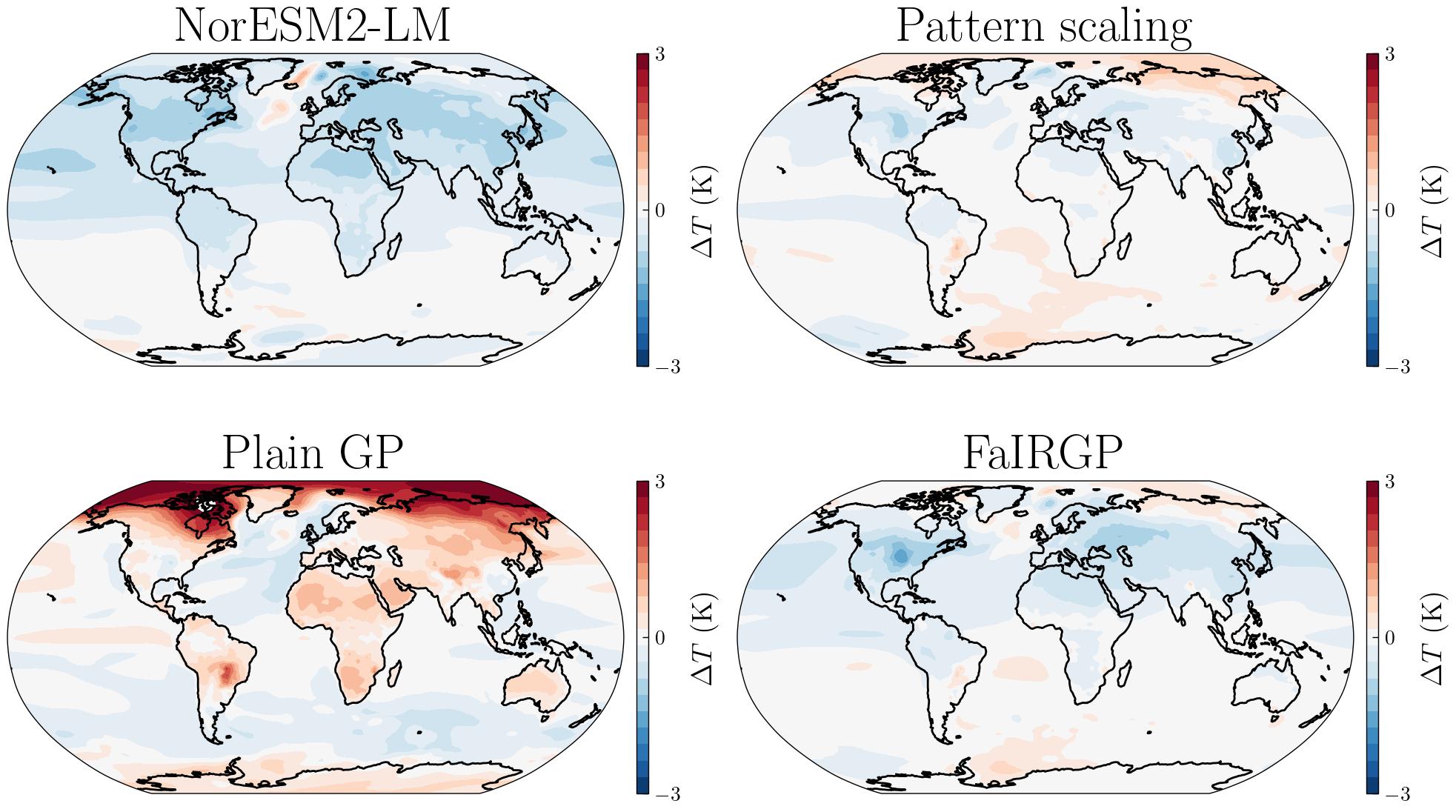
Figure 11: Maps of surface temperatures averaged for the hist-aer experiment averaged over 1900-2014 period. Top-Left: Groundtruth NorESM2-LM surface temperatures map. Top-Right: Prediction with the FaIR pattern scaling baseline. Bottom-Left: Prediction with Plain GP posterior mean. Bottom-Right: Prediction with the FaIRGP posterior mean.

Appendix C Complementary material on Gaussian processes

C.1 Additional illustrations for Gaussian processes

We provide here additional illustrations to develop intuition on how GPs can be used for a regression task. Consider a simple regression problem $y={\mathsf{f}}(x)+\upvarepsilon$ where $\upvarepsilon\sim{\mathcal{N}}(0,\sigma^{2})$. Let $k(x,x^{\prime})$ be a user-specified covariance function, and suppose we place a prior ${\mathsf{f}}(x)\sim{\operatorname{GP}}(0,k)$.

Figure 12 plots the mean function and the 95% credible interval that results from our choice of prior over the regression function. Since this is effectively a probability distribution over functions, we can draw samples from it. Figure 13 shows the plots of 10 functions samples from this distribution.

Figure 12: Plot of the ${\mathsf{f}}(x)\sim{\operatorname{GP}}(0,k)$ prior mean function and 95% confidence region.

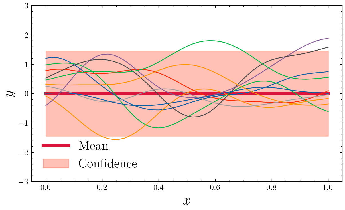
Figure 13: Same Figure 12, but plotting on top functions that are samples from the distribution over functions specified by ${\mathsf{f}}(x)\sim{\operatorname{GP}}(0,k)$.

Figure 14 shows how the prior can be updated with observations of $y$, thereby updating it into a posterior. Because the posterior is still a probability distribution, we can still draw samples from it as shown in Figure 15. However, the functions drawn are now constrained by the data and provide a better fit to observations. The posterior GP therefore induces a probability distribution over functions that provide a sound fit to observations

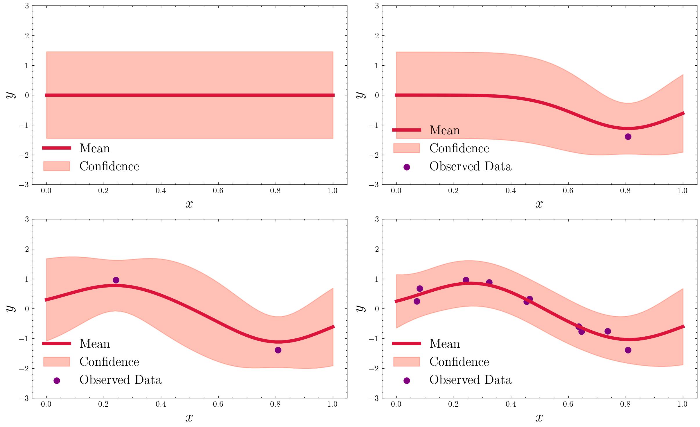
Figure 14: Plots of the posterior mean function and posterior 95% credible interval when updating the prior with 0, (top-left), 1 (top-right), 2 (bottom-left) and 10 (bottom-right) observations.

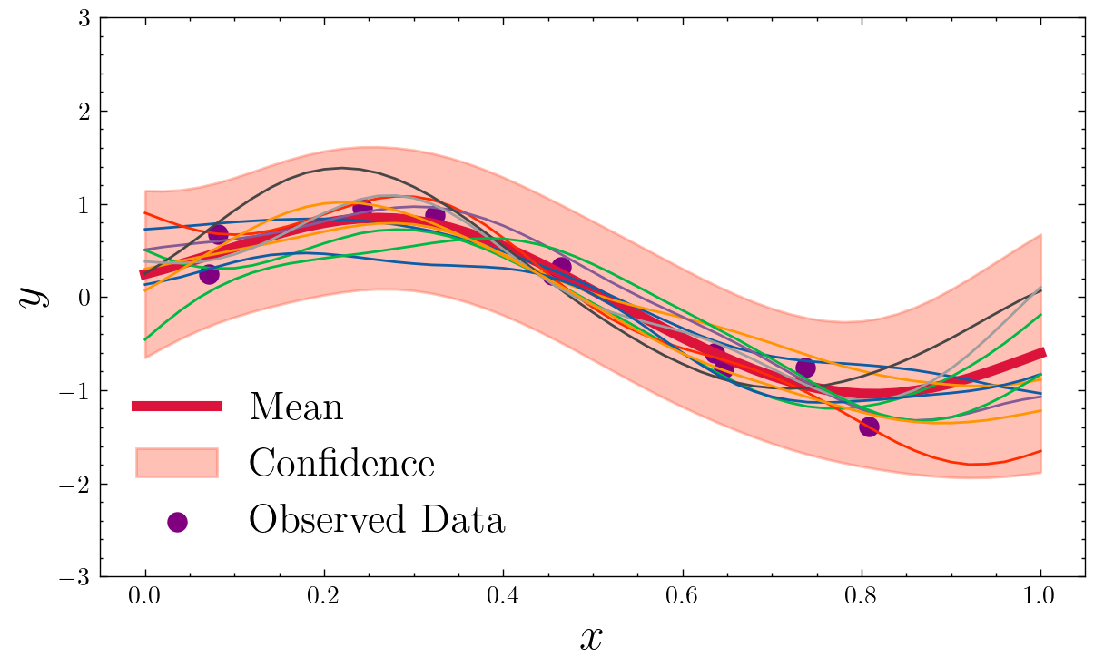
Figure 15: Plots of the posterior mean function and posterior 95% credible interval with 10 observations + plots of functions sampled from the posterior distribution specified over functions.

C.2 Matérn covariance

The Matérn covariances are a class of stationary covariance functions widely used in spatial statistics. The Matérn-$\nu$ covariance between two points $x,x^{\prime}\in{\mathbb{R}}$ is given by

$$C_{\nu}(x,x^{\prime})=\frac{2^{1-\nu}}{\Gamma(\nu)}\left(\sqrt{2\nu}\frac{|x-x^{\prime}|}{\ell}\right)^{\nu}K_{\nu}\left(\sqrt{2\nu}\frac{|x-x^{\prime}|}{\ell}\right),$$ (94)

where $\Gamma$ is the gamma function, $K_{\nu}$ is the modified Bessel function and $\ell>0$ is a lengthscale hyperparameter.

The covariance function expression considerably simplifies for $\nu=p+1/2$ where $p\in{\mathbb{N}}$. For example, for $\nu=1/2$ ($p=0$) and $\nu=3/2$ ($p=1$) we have

$$C_{1/2}(x,x^{\prime}) =\exp\left(-\frac{|x-x^{\prime}|}{\ell}\right)$$ (95)

$$C_{3/2}(x,x^{\prime}) =\left(1+\sqrt{3}\frac{|x-x^{\prime}|}{\ell}\right)\exp\left(-\sqrt{3}\frac{|x-x^{\prime}|}{\ell}\right)$$ (96)

When $x,x^{\prime}\in{\mathbb{R}}^{d}$, the distance $|x-x^{\prime}|$ can be substituted by the norm $\|x-x^{\prime}\|=\sqrt{\sum_{i=1}^{d}(x_{i}-x_{i}^{\prime})^{2}}$. The covariance is called an automatic relevance determination (ARD) kernel when each dimension has its own independent lengthscale parameter $\ell_{i}>0$. For example, the Matérn-$1/2$ and Matérn-$3/2$ ARD kernel write

$$C_{1/2}(x,x^{\prime}) =\exp\left(-\sqrt{\sum_{i=1}^{d}\frac{(x_{i}-x_{i}^{\prime})^{2}}{\ell_{i}^{2}}}\right)$$ (97)

$$C_{3/2}(x,x^{\prime}) =\left(1+\sqrt{3\sum_{i=1}^{d}\frac{(x_{i}-x_{i}^{\prime})^{2}}{\ell_{i}^{2}}}\right)\exp\left(-\sqrt{3\sum_{i=1}^{d}\frac{(x_{i}-x_{i}^{\prime})^{2}}{\ell_{i}^{2}}}\right).$$ (98)

When a Matérn-$p+1/2$ covariance function is used as a kernel for a GP, draws from the GP are $p$ times continuously differentiable (with convention that $0$ times means simply continuous).