TUNeS: A Temporal U-Net with Self-Attention for Video-based Surgical Phase Recognition

Abstract

To enable context-aware computer assistance in the operating room of the future, cognitive systems need to understand automatically which surgical phase is being performed by the medical team. The primary source of information for surgical phase recognition is typically video, which presents two challenges: extracting meaningful features from the video stream and effectively modeling temporal information in the sequence of visual features. For temporal modeling, attention mechanisms have gained popularity due to their ability to capture long-range dependencies. In this paper, we explore design choices for attention in existing temporal models for surgical phase recognition and propose a novel approach that uses attention more effectively: TUNeS, an efficient and simple temporal model that incorporates self-attention at the core of a convolutional U-Net structure. In addition, we propose to train the feature extractor, a standard CNN, together with an LSTM on preferably long video segments, i.e., with long temporal context. In our experiments, all temporal models performed better on top of feature extractors that were trained with longer temporal context. On these contextualized features, TUNeS achieves state-of-the-art results on the Cholec80 dataset.

IEEEexample:BSTcontrol

action segmentation, attention, Cholec80, sequence modeling, surgical phase, surgical workflow

1 Introduction

Video-based surgical phase recognition refers to automatically analyzing the video stream that is recorded in the operating room to recognize which surgical phase [1] is being performed. Robust and accurate methods for surgical phase recognition are a prerequisite for computer-assisted surgery, where context-aware assistance functions are to be provided automatically [2]. Here, automatic computer assistance could comprise, for example, providing crucial patient-related information at the right time (intra-operatively) or preparing the surgical report (post-operatively).

Current approaches for surgical phase recognition follow a data-driven approach, meaning that they learn from annotated example videos. Typically, two types of deep-learning models are combined: (i) a visual feature extractor, e.g., a Convolutional Neural Network (CNN) or a Vision Transformer (ViT) [3], and (ii) a temporal model, e.g., a Temporal Convolutional Network (TCN) [4, 5] or a Recurrent Neural Network (RNN). An RNN typically consists of Long Short-Term Memory (LSTM) cells [6] or Gated Recurrent Units (GRUs) [7]. Recent temporal models also integrate attention mechanisms [8, 9].

In general, the feature extractor learns to extract descriptive features from individual video frames. Based on that, the temporal model learns to identify meaningful temporal patterns in the sequence of visual features to identify the surgical phases. For handling long surgical videos, the temporal model should be able to capture long-range temporal relationships.

1.0.1 Visual feature extraction

The question of how to obtain suitable features for phase recognition has not been studied extensively so far. Most methods simply finetune a CNN, typically a ResNet [10], on the task of phase recognition after pre-training on a large-scale dataset. Few studies [11, 12] investigated other architectures such as ViTs or spatio-temporal video models. Others explored training a standard CNN either on additional tasks, e.g., tool recognition [13, 14], surgical step recognition [15], or surgical scene segmentation [16], or on self-supervised objectives [17, 18, 19].

Inspired by the performance of simple end-to-end CNN-LSTM models on the phase recognition task [20, 21], we propose to train the feature extractor, a standard CNN, in context by combining it with an LSTM network and training both components jointly on truncated video sequences (up to 64 frames) (see section 4.1). Training with temporal context rewards the CNN to extract features that could prove useful in hindsight and enables the CNN to tolerate ambiguous frames, relying on the temporal model to resolve these. After training, features are extracted using the CNN only.

1.0.2 Modeling long-range relationships

Attention mechanisms [8] were designed to model global relations in sequences. By stacking attention and feedforward neural networks, the Transformer [9] achieved break-through results on sequence modeling tasks. Inspired by this success, researchers incorporated attention in temporal models for phase recognition as well [22, 23, 24, 25] (see Fig. 2, section 3.2). Yet, these models do not necessarily use attention in an efficient and effective way. For example, some models reverted to local attention, which is computed within limited time windows only – thus counteracting the idea of modeling global dependencies.

In contrast, we propose to integrate attention at the core of a convolutional encoder-decoder architecture (see Fig. 2f, section 4.2). Here, features are semantically rich and downsampled along the temporal dimension so that attention can be computed efficiently and without additional hand-crafted constraints. The proposed model, named TUNeS (Temporal U-Net with Self-Attention), is suited for both online and offline phase recognition.

1.0.3 Evaluation

We conducted a large number of experiments to demonstrate the positive effects of training the feature extractor with long temporal context (see Fig. 6). Our experiments also show that TUNeS compares favorably to many baseline methods, in terms of both recognition accuracy and computational efficiency (see Fig. 6 and Fig. 7). TUNeS, combined with a feature extractor that is trained with long temporal context, achieves state-of-the-art results on Cholec80. Source code will be made available.

2 Background

2.1 Surgical phase recognition

Given a video $v$ of length $T$, phase recognition is the task to estimate which phase $p$ is being executed at any time $t$. Here, $p$ is one of $C$ predefined surgical phases.

We denote the true phase that is happening at time $t$ as $y_{t}$, $1\leq y_{t}\leq C$, and the sequence of all ground truth phase labels as $\left(y_{t}\right)_{1\leq t\leq T}$ or simply $y_{1:T}$. The estimate of the phase at time $t$, computed by an automatic algorithm, is $\hat{y}_{t}\in\mathbb{R}^{C}$. Here, $\hat{y}_{t,p}$ is the computed score for the event that $y_{t}$ equals phase $p$. The video itself is a sequence of video frames $v_{t}$.

For intra-operative applications, phase recognition needs to be performed online. Here, only video frames $v_{t^{\prime}}$ up until the current time $t$, i.e., $t^{\prime}\leq t$, can be analyzed to estimate the current phase. For post-operative applications, however, offline recognition is feasible. Here, information from all frames in the video can be processed to estimate the phase at any time.

(a) Transformer block [9]

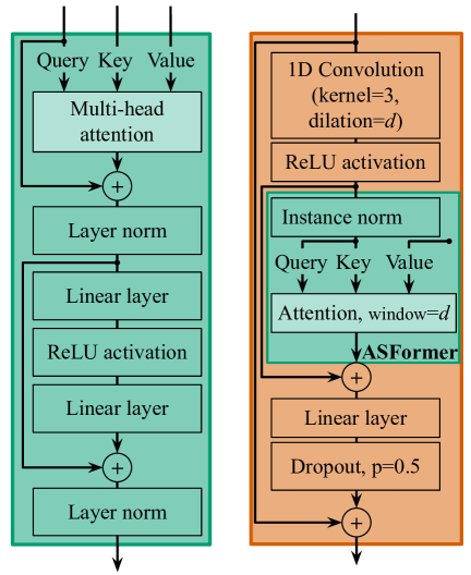
(b) Layer in MS-TCN [5] and ASFormer [24]

Figure 1: Building blocks of related architectures. ASFormer adds an attention mechanism between the convolution and the fully connected layer of the MS-TCN layer.

2.2 Attention mechanism

Let $Q=q_{1:S}$ be a sequence of queries and $U=u_{1:T}$ be a sequence of values, which is associated with a sequence $K=k_{1:T}$ of keys, i.e., $k_{t}$ is the key of $u_{t}$. In an attention mechanism [8], each element $q_{s}\in Q$ collects information from any element $u_{t}\in U$ by computing an attention-weighted sum over the complete sequence $U$:

$$\begin{split}\mathrm{Attention}(Q,K,U)&=\left(x_{s}\right)_{1\leq s\leq S},\text{ where }\\ x_{s}&=\sum_{t}\frac{\exp{\alpha(q_{s},k_{t})}}{\sum_{t^{\prime}}\exp{\alpha(q_{s},k_{t^{\prime}})}}\cdot u_{t}\end{split}$$ (1)

The weights in this sum are the attention weights $\alpha(q_{s},k_{t})$ after Softmax. Here, function $\alpha$ is trained to determine how relevant the element with key $k_{t}$ is given query $q_{s}$.

In practice, $Q$, $K$, and $U$ are passed through trainable linear layers before computing attention, and $\alpha$ simply computes the scaled dot product. In multi-head attention, multiple linear layers are used so that attention is computed on multiple representation subspaces in parallel. In the case of self-attention, $Q$, $K$, and $U$ all refer to the same sequence. [9]

Attention weights may be masked, i.e., set to $-\infty$, according to specific rules: Local attention is only computed within local time windows of size $1+2\omega$, i.e., $\alpha(q_{s},k_{t})=-\infty$ for all $t$ with $|t-s|>\omega$. Causal attention does not allow attending to future sequence elements, thus $\alpha(q_{s},k_{t})=-\infty$ for all $t$ with $t>s$.

In the Transformer architecture [9], attention is embedded in Transformer blocks with residual connections and normalization layers (Fig. 1a). The attention mechanism is followed by a feedforward network, which consists of two linear layers with a nonlinearity in between.

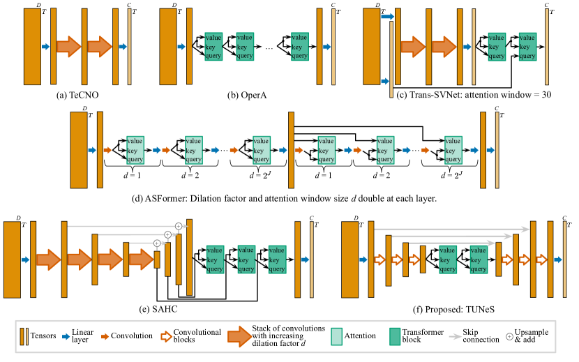
Figure 2: Overview of temporal models for surgical phase recognition with a focus on how they incorporate attention mechanisms.

3 Related work

3.1 Phase recognition without attention mechanisms

Early models for video-based phase recognition consisted of a CNN for feature extraction and an LSTM network as temporal model [26, ch. 6.4]. Later, Czempiel et al. [14] proposed TeCNO for temporal modeling. TeCNO is a TCN with multiple stages (MS-TCN [5]), where subsequent stages refine predictions of previous stages. Each stage consists of several layers with dilated temporal convolutions (Fig. 1b), where the dilation factor doubles at each layer. For online recognition, causal dilated convolutions [27] are used, i.e., convolutions are computed over the current and preceding time steps only. Yi et al. [28] suggested to train multi-stage models not end-to-end, but to apply disturbances to the intermediate predictions during training. Recently, Kadkhodamohammadi et al. [29] introduced PATG, which uses a SE-ResNet as feature extractor and a graph neural network as temporal model. Zhang et al. [30] proposed a reinforcement learning approach to retrieve phase transitions for offline recognition.

Whereas feature extractor and temporal model were trained separately in these studies, others proposed to train both models jointly on truncated video sequences. Jin et al. [20] trained SV-RCNet, a ResNet-LSTM, end-to-end on video sequences with a duration of 2 s. Later, they proposed TMRNet [31], which augments a ResNeSt-LSTM with a long-range memory bank [32] so that additional feature vectors from the previous 30 s can be queried. Recently, Rivoir et al. [21] showed that CNN-LSTMs should be trained on even longer video sequences, which becomes feasible only if effects caused by Batch Normalization (BN) are taken into account. They trained their best model, a ConvNeXt-LSTM, on sequences of 256 s.

Paper contribution

We employ an end-to-end ResNet-LSTM to train a standard ResNet with extended temporal context for visual feature extraction. To train the ResNet-LSTM on long video sequences despite ResNet’s potentially problematic BN layers, we use a simpler approach than [21]: We make sure that the training batches are diverse enough by sampling many (at least ten) video sequences per batch from throughout the training data. To model global dependencies and for offline recognition, we still suggest to train an additional temporal model on the extracted feature sequences in a second step.

3.2 Phase recognition with attention mechanisms

To model long-range dependencies, recent studies proposed to integrate attention mechanisms into temporal models (Fig. 2). With attention, an element $q_{s}$ in the query sequence can be related to any element $u_{t}$ in the value sequence, regardless of their temporal distance $|t-s|$. In contrast, RNNs process sequences sequentially, relying on a fixed-sized hidden state to retain relevant information, and temporal convolutions process information in local neighborhoods only. Thus, information needs to travel through several layers of convolutions to become available at temporally distant locations.

Czempiel et al. [22] presented OperA, a stack of Transformer blocks, for online recognition (Fig. 2b). This approach uses only self-attention to model temporal dependencies and thus may be lacking a notion of locality and temporal order. Because the model seemed to struggle to filter relevant information from the feature sequences, the authors proposed to train with a special attention regularization loss.

Gao et al. [23] introduced Trans-SVNet for online recognition (Fig. 2c), which adds two Transformer blocks on top of a frozen TeCNO model. The first block computes self-attention on the TeCNO predictions. In the second block, the initial predictions of the feature extractor attend over the output of the first Transformer block. All attention operations are computed locally, using the feature vectors of the previous 30 s only.

Yi et al. [24] proposed ASFormer, an offline model for temporal action segmentation (Fig. 2d). This model integrates attention into MS-TCN layers (Fig. 1b), where the convolutions help to encode local inductive bias. Again, attention is computed within local windows. Here, the window size equals the dilation factor $d$ of the convolution, which doubles at each layer. Recently, Zhang et al. [33] suggested to add a MS-TCN stage in parallel to the first ASFormer stage and to fuse their outputs. Chen et al. [34] presented an online two-stage version of ASFormer, where the dilation factors in the second stage halve (instead of double) at each layer. Restricting attention to local neighborhoods of a predefined size seems to help with handling the complexity of long, noisy feature sequences but hinders the modeling of global dependencies.

Whereas previous models incorporated hierarchical patterns only implicitly, namely by means of doubling dilation factors, Ding and Li [25] proposed an explicitly hierarchical model: SAHC (Fig. 2e). This model uses MS-TCN-like stages to process feature sequences, which are downsampled progressively. Then, the computed multi-scale feature maps are fused from coarse to fine like in a Feature Pyramid Network. Transformer blocks with global attention are integrated at the very end of the model, where the final high-resolution sequence queries further information from the lower-resolution sequences.

Paper contribution

We argue that Transformer blocks should be integrated differently into temporal models to fully exploit their expressive long-term modeling capabilities:

Unlike SAHC, Transformer blocks should be positioned directly after the downsampling path so that global dependencies are analyzed earlier and can be further refined in the upsampling path. By also distributing the number of convolutions evenly between downsampling and upsampling path, we obtain a symmetric U-Net [35, 36] structure with few parameters and powerful Transformer blocks at the bottleneck: TUNeS, as outlined in Fig. 2f.

Unlike OperA, which applies attention directly to the raw and typically noisy feature sequences, TUNeS applies attention to the pre-filtered, semantically rich features after the encoder. On these high-level features, attention is presumably more effective so that additional constraints can be avoided, such as the attention regularization loss (OperA) or the fallback to local attention (ASFormer, Trans-SVNet), which would prevent modeling global relations. Due to the quadratic complexity of attention, it is also computationally beneficial to compute attention only on the high-level feature maps, which are downsampled by an order of magnitude.

Previously, U-Nets with self-attention at the bottleneck were also used successfully for image generation with autoregressive models [37] or diffusion models [38], for image segmentation [39, 40], and for speech denoising [41].

4 Methods

4.1 Feature extractor with temporal context

We use a standard CNN as feature extractor: ResNet-50 [10], pre-trained on ImageNet. However, we train the CNN not on individual video frames (Fig. 3a) but with temporal context. For this purpose, we add an LSTM cell with 512 hidden units, which processes the sequence of computed CNN features. The CNN-LSTM is trained end-to-end on sequences of $L$ consecutive frames (Fig. 3b). Here, we minimize the cross-entropy loss, computed on all $L$ frames in the sequence.

To train on a balanced set of video sequences, we sample five sequences from each phase and one sequence around each phase transition from each video during one training epoch. To avoid BN-related problems, video sequences are processed in appropriately large batches of $B\times L$ frames, $B\geq 10$.

After training, only the CNN is used to extract features: For each frame $v_{t}$, we obtain the feature vector $f_{t}\in\mathbb{R}^{D}$, $D=2048$, after the ResNet’s global average pooling layer.

(a)

(b)

Figure 3: Feature extractor training: (a) Training the CNN on individual video frames. The fully connected (FC) layer acts as linear classifier on top of the extracted feature vector $f_{t}$. (b) Training the CNN with temporal context, using an LSTM cell to model temporal relationships.

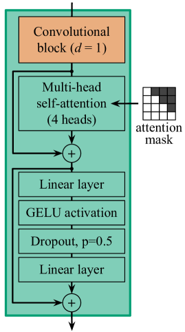
(a)

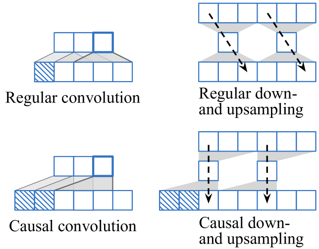
(b) Regular vs. causal operations

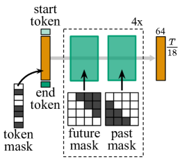
(c) Alternate attention masking

Figure 4: (a) TUNeS Transformer block. (b) Illustration of regular and causal convolutions (left) and downsampling operations (right). Padded elements are depicted as cross-hatched squares. Grey trapezoids relate inputs to outputs and thus indicate dependencies ($\dashrightarrow$). Sequences are processed from bottom to top. (c) In offline mode, TUNeS Transformer blocks alternately process information from the past or from the future.

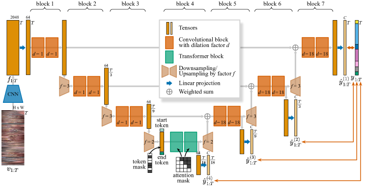
Figure 5: TUNeS is a U-Net of temporal convolutions, which can be coarsely divided into seven TUNeS blocks. To model long-range dependencies, self-attention is used at the bottleneck (block 4). TUNeS processes the sequence of visual features $f_{1:T}$, which is obtained by applying the frozen feature extractor (see section 4.1) to every frame $v_{t}$ in input video $v$. Multi-scale phase predictions $\hat{y}_{1:T}^{(i)}$ are extracted from the U-Net decoder.

4.2 Temporal U-Net with self-attention

TUNeS follows a U-Net structure [35, 36] (Fig. 5). In the encoder, the feature sequence $f_{1:T}$ is repeatedly passed through temporal convolutions and downsampled. In the decoder, the sequence is repeatedly upsampled and passed through further convolutions. At the bottleneck, Transformer blocks with self-attention are used to enrich the sequence with global context. Here, the downsampled feature sequence is treated as a sequence of tokens, to which start and end tokens are added.

In the decoder, the intermediate feature sequence is enriched with the information of higher-resolution feature maps by means of skip connections to the encoder. Here, the sum in each skip connection is weighted with a learnable scalar. Further, linear classifier heads after each decoder block compute phase predictions $\hat{y}^{(i)}$ at multiple temporal scales.

In the encoder, regular convolutions ($d=1$) are used. In the decoder, dilated convolutions ($d=18$) are used to retain a large receptive field when progressing to higher-resolution sequences. Here, we set $d=18$ because the coarsest, highest-level feature maps are downsampled by a factor of $18$.

4.2.1 Architecture details

Down- und upsampling by factor f is implemented using 1D convolutions with kernel f and stride f, where the convolution is transposed for upsampling. The convolutional block corresponds to a MS-TCN layer (Fig. 1b) with GELU [42] activation. The TUNeS Transformer block (Fig. 4a) computes multi-head self-attention and starts with a convolutional block to add local inductive bias [24]. This convolutional block acts as position encoding generator, which adds conditional positional encodings [43] to the input.

Like MS-TCN, TUNeS does not include any normalization layers. Each operation, including each attention head, processes and outputs sequences with $\mathrm{dim}=64$ channels.

4.2.2 Causal operations for online recognition

To be applicable to online recognition, it is required that the temporal model does not access future information. Thus, TUNeS uses causal convolutions for online recognition like TeCNO [14]. In addition, causal self-attention is computed in the Transformer blocks by applying a causal mask to the attention weights.

It is important to perform the downsampling operations in a causal way as well. Like for convolutions, this can be implemented by shifting input sequences by $k-1$ elements to the right, which corresponds to adding $k-1$ padded elements at the left (Fig. 4b). Here, $k$ is the size of the kernel. In contrast, regular downsampling would leak future information. In that case, an element in the output sequence could depend on up to $k-1$ future elements in the input sequence.

4.2.3 Alternate attention masking for offline recognition

When computing global self-attention in offline mode, it may be difficult to correctly separate past from future information. To help with this, we alternately prevent access to future and to past elements in the TUNeS Transformer blocks (Fig. 4c). Further, we found it beneficial to increase the number of Transformer blocks for offline recognition from two to eight.

4.2.4 Training objective

Let $\left\{\hat{y}^{(i)}:1\leq i\leq 4\right\}$ be the multi-scale phase predictions, where the length of each prediction $\hat{y}^{(i)}$ is reduced by factor $\chi_{i}$ and $\chi=(1,3,9,18)$. For $2\leq i\leq 4$, we compute downsampled ground truth labels $y^{(i)}$ by applying one-hot encoding to $y$, followed by max pooling with kernel $\chi_{i}$ and stride $\chi_{i}$.

We compute losses at all scales, using cross-entropy (CE) loss for the full-resolution prediction $\hat{y}^{(1)}$ and binary cross-entropy (BCE) loss for the lower-resolution predictions, see (2) and appendix .1.9. BCE is used because downsampled annotations assign multiple correct labels to downsampled time steps that coincide with phase transitions.

$$\begin{split}\mathcal{L}_{\text{total}}=&\mathcal{L}_{\text{phase}}(\hat{y}^{(1)},y)+\sum_{k=2}^{4}\mathcal{L}_{\text{BCE}}(\hat{y}^{(k)},y^{(k)})\\ &\mathcal{L}_{\text{phase}}(\hat{y},y)=\mathcal{L}_{\text{CE}}(\hat{y},y)+\lambda_{\text{smooth}}\cdot\mathcal{L}_{\text{smooth}}(\hat{y})\end{split}$$ (2)

To counter class imbalance, we use class weights $\gamma$, which are computed on the training data following the median frequency balancing [44] approach. In addition, we compute a smoothing loss $\mathcal{L}_{\text{smooth}}$ [5] on the full-resolution prediction, which is weighted by factor $\lambda_{\text{smooth}}=0.15$.

Figure 6: Surgical phase recognition results on the Cholec80 dataset (32:8:40 split). We present the feature extractor’s standalone performance as well as the performance of various temporal models, trained on top of the frozen feature extractor. Error bars indicate the standard deviation over repeated experimental runs. The asterisk* indicates training without feature sequence augmentation and smoothing loss. Numerical results can be found in the appendix (Tables 4 and 5).

4.2.5 Regularization

For data augmentation, we augment feature sequences by (i) shifting the complete sequence to the right by a small random number of time steps and by (ii) increasing and decreasing the video speed by randomly dropping and duplicating elements of the feature sequence.

In addition, we mask spans in the token sequences that are input to the Transformer blocks, inspired by the pre-training procedures for masked language models [45, 46]. Here, we randomly sample masks to cover spans that correspond to 18–300 s in the full-resolution video. However, we make sure that phase transitions are not masked because it would be impossible to reconstruct their exact timing. In total, around 35% of all tokens are masked per sequence.

5 Experiments

5.1 Dataset and evaluation metrics

Experiments were conducted on the Cholec80 dataset [13]. Cholec80 consists of 80 video recordings of laparoscopic gallbladder removals, which are labeled with phase and tool information. Here, $C=7$ different surgical phases are annotated. We used only the phase labels to train feature extractors and temporal models. The videos were processed at a temporal resolution of 1 fps. Unless stated otherwise, experiments were performed on the 32:8:40 data split, meaning that the first 32 videos in Cholec80 were used for training, the next 8 videos for validation, and the last 40 videos for testing. In particular, hyperparameters were tuned on the validation subset.

We use the following evaluation metrics: Video-wise accuracy, video-wise Macro Jaccard (or Intersection over Union), and $\mathit{F1}$ score, which is computed as the harmonic mean of the mean video-wise Precision and the mean video-wise Recall. The Macro Jaccard for one test video is the average of the phase-wise Jaccard scores computed on this video. To avoid problems with undefined values, we omit the phase-wise scores for phase $p$ and video $v$ if $p$ is not annotated in $v$.

For comparison with prior art, we also report the relaxed evaluation metrics $\mathcal{R}\text{-}\mathsf{Jaccard}$ (or $\mathcal{R}\text{-}\mathsf{Precision}$ and $\mathcal{R}\text{-}\mathsf{Recall}$) and $\mathcal{R}\text{-}\mathsf{Accuracy}$, which were proposed to tolerate certain errors within 10 s before or after an annotated phase transition. For all metrics, we used the implementation provided by [47].

Figure 7: Performance measurements for processing feature sequences of increasing duration with different temporal models in offline mode. We also present the number of parameters for each temporal model.

5.2 Comparisons to baselines and state of the art

We conducted experiments 1) to explore the impact of providing longer temporal context when training the visual feature extractor, and 2) to compare TUNeS to an extensive number of established temporal models.

5.2.1 Feature extractors

We trained feature extractors with context lengths $L$ of 1, 8, or 64 frames (Fig. 6). The feature extractor with $L=1$ is simply a ResNet-50, without the LSTM on top (Fig. 3a). Following the custom sampling strategy (section 4.1), 1264 video sequences were processed in each epoch, for any size of $L$. With $L=64$, we trained the feature extractor for 200 epochs. For comparability, we trained the feature extractor with $L=8$ for 1600 epochs and with $L=1$ for 12800 epochs. Thus, all feature extractors see the same number of video frames during training, but in different contexts and in different order. The batch size $B$ was 10 video sequences with $L=64$, 80 with $L=8$, and 128 video frames with $L=1$.

To assess the feature extractor’s abilities when $L>1$, we used the predictions of the jointly trained LSTM: To infer the current phase, we applied the CNN-LSTM to the $L-1$ previous and to the current frame and took the final prediction. In addition, we performed carry-hidden evaluation (CHE) [21], where the LSTM’s hidden state is carried through the video.

To account for the randomness in training deep-learning models, experiments were repeated five times using different random seeds.

Table 1: Online recognition on Cholec80 (40:40 split). Comparison to results from the literature.

Model	$\mathcal{R}\text{-}\mathsf{Accuracy}$		$\mathcal{R}\text{-}\mathsf{Jaccard}$
	$M$	$SD_{V}$	$M_{P}$	$SD_{P}$
ResNet-50–LSTMb, $L=8$ (similar to SV-RCNet[20])	0.881	0.063	0.739	0.090
TeCNO [14], results of [23]	0.886	0.078	0.751	0.069
TMRNet w/ ResNeST [31]	0.901	0.076	0.791	0.057
Trans-SVNet [23]	0.903	0.071	0.793	0.066
Not E2E [28]	0.920	0.053	0.771	0.115
SAHC [25]	0.918	0.081	0.812	0.055
ConvNeXt–LSTMb, $L=256$ [21]	0.935	0.065	0.829	0.101
TUNeS, $L=64$	0.939	0.050	0.842	0.083
Like prior art, we report the mean $M$ and the standard deviation over videos $SD_{V}$ for $\mathcal{R}\text{-}\mathsf{Accuracy}$. For $\mathcal{R}\text{-}\mathsf{Jaccard}$, we report the mean over phase-wise means $M_{P}$ and the standard deviation over phases $SD_{P}$.

(a)

Model	Accuracya	Macro Jaccarda	$\mathit{F1}$ scorea
ResNet-50–LSTMb, $L=8$	0.872 $\pm$ 0.004	0.707 $\pm$ 0.007	0.832 $\pm$ 0.003
TeCNO [14]
results of [11]	0.874 $\pm$ 0.014	–	0.825 $\pm$ 0.018
results of [34]	0.900	0.723	0.839
Trans-SVNet [23]
results of [34]	0.896	0.731	0.845
GRU w/ VideoSwin [12]	0.909	–	0.853
PATG w/ SE- ResNet-50 [29]	0.914	–	0.854
Dual Pyramid ASFormer w/ PCPVT [34]	0.914	0.754	0.858
TUNeS, $L=64$	0.927 $\pm$ 0.004	0.799 $\pm$ 0.005	0.890 $\pm$ 0.003
aThe reported sample standard deviation refers to the variation over repeated experimental runs.
bTrained end-to-end on short video sequences of $L$ frames.

(b)

Table 2: Offline recognition on Cholec80. Comparison to results from the literature.

Model $\mathcal{R}\text{-}\mathsf{Accuracy}$ $\mathcal{R}\text{-}\mathsf{Precision}$ $\mathcal{R}\text{-}\mathsf{Recall}$ split $M$ $SD_{V}$ $M_{P}$ $SD_{P}$ $M_{P}$ $SD_{P}$ ASTCFormer [33] 0.957 0.033 0.923 0.062 0.912 0.095 40:20:20 TUNeS, $L=64$ 0.964 0.022 0.936 0.070 0.939 0.054 40:20:20 Like prior art, we report the mean $M$ and the standard deviation over videos $SD_{V}$ for $\mathcal{R}\text{-}\mathsf{Accuracy}$. For $\mathcal{R}\text{-}\mathsf{Precision}$ and $\mathcal{R}\text{-}\mathsf{Recall}$, we report the mean over phase-wise means $M_{P}$ and the standard deviation over phases $SD_{P}$.

(a)

Model Accuracy^a Macro Jaccard^a $\mathit{F1}$ score^a split GRU w/ VideoSwin [12] 0.939 – 0.898 40:40 TUNeS, $L=64$ 0.949 $\pm$ 0.005 0.836 $\pm$ 0.009 0.912 $\pm$ 0.005 40:40 Transition Retrieval Network [30] 0.901 – 0.848 40:20:20 TUNeS, $L=64$ 0.953 $\pm$ 0.004 0.837 $\pm$ 0.011 0.911 $\pm$ 0.007 40:20:20 ^aThe reported sample standard deviation refers to the variation over repeated experimental runs.

(b)

5.2.2 Temporal models

For each context length $L\in\{1,8,64\}$, we trained TUNeS and a variety of other temporal models on the extracted feature sequences (Fig. 6). The baseline models included an RNN (2-layer GRU), a TCN (TeCNO), and models that integrate attention in different ways (OperA, SAHC, ASFormer). For comparability, we set the hidden dimension of all temporal models to $\mathrm{dim}=64$. To account for random effects, we repeated each experiment five times on each of the five feature extractor instances, yielding 25 experimental runs.

All temporal models were trained for 75 epochs using the Adam [48] optimizer and a batch size of one feature sequence. Baseline models were trained on the combined loss $\mathcal{L}_{\text{phase}}$ with $\lambda_{\text{smooth}}=0.15$. For models with multiple stages (TeCNO, SAHC, ASFormer), we computed the loss on the output of all stages. Feature sequence augmentation was applied as described in section 4.2.5. Gradients were clipped to have a maximum norm of 1. Finally, we selected the model that achieved the highest Macro Jaccard on the validation set.

To select an appropriate learning rate $\eta$ for each model, we ran a quick sweep over $\eta\in\{10^{-4},3\cdot 10^{-4},5\cdot 10^{-4},10^{-3}\}$. Usually, $\eta=5\cdot 10^{-4}$ worked well. If available, we tried to consider the training strategy of the original code base. Full training details are described in appendix .1.

5.2.3 Performance measurements

For TUNeS as well as for the baselines, we measured model latency and peak GPU memory allocation in offline mode. To this end, we used synthetic feature sequences, which are randomly initialized tensors of dimension $T\times 2048$, with a length $T$ of 450, 900, 1800, 3600, and 7200 frames. Fig. 7 presents the mean of 1000 measurements, after taking 100 measurements for warm-up.

5.2.4 Comparison to the state of the art

We compare the results of TUNeS, trained on features with maximum context $L=64$, with previously reported results on the 40:40 split (Tables 1 and 2). Here, the feature extractor with $L=64$ and TUNeS were re-trained on all of the first 40 videos in Cholec80. Due to the lack of a validation set, we selected the model after the last epoch for testing. To improve convergence, we continuously reduced the learning rate during training, following a cosine annealing schedule [49]. For comparisons on the 40:20:20 split, we evaluated the models trained for the 40:40 split on the last 20 videos in Cholec80.

Figure 8: Impact of integrating Transformer blocks at different positions in the TUNeS model. Left: Results on the Cholec80 dataset (32:8:40 split). Error bars indicate the standard deviation over repeated experimental runs. Right: Performance measurements in offline mode.

Discussion

Training the feature extractor in context proved beneficial: The standalone performance of the feature extractor improved as the temporal context increased. In addition, all temporal models performed better on top of feature extractors that were trained with longer temporal context (Fig. 6). Yet, we simply used ResNet-50 for feature extraction as opposed to a more powerful ViT or the more advanced ConvNeXt.

Apparently, training in context helps the CNN to learn meaningful, contextualized features that hold crucial information for subsequent analysis. Yet, training in context is simple to implement and does not require additional manual annotations such as tool labels. Also, it does not take more time than the standard frame-wise training. The only requirement is sufficient GPU memory (32 GB in our experiments).

When evaluating the baselines (Fig. 6), we found that the 2-layer GRU and OperA achieved subpar results. For the GRU, we suspect that regularization with the smoothing loss and the proposed feature sequence augmentation is not as effective for a recurrent model. For OperA, we presume that the model is suffering from a lack of local inductive bias and struggles to filter information from noisy features. Yet, OperA improves considerably on contextualized features ($L=64$), which might be more meaningful and thus easier to analyze with attention. Please note that we used a custom implementation of OperA because official code has not been released yet.

Further, training Trans-SVNet on top of TeCNO improved the results only marginally. Yet, compared to the original code base, we used different hyperparameters for TeCNO (9 layers per stage, $\mathrm{dim}=64$) and trained TeCNO for up to 75 epochs instead of only 8. We assume that Trans-SVNet mostly learns to locally smooth the TeCNO outputs, which may not be necessary if TeCNO was tuned and trained properly.

The best performing baselines were TeCNO, SAHC, and ASFormer. TUNeS outperformed the baselines in terms of accuracy and scored better or similarly on Macro Jaccard (Fig. 6, Tables 4 and 5). The results achieved by TUNeS, trained on top of the feature extractor with $L=64$, also compare favorably to previous results from the literature (Tables 1 and 2). Moreover, TUNeS is computationally efficient and scales well on long sequences of up to two hours, regarding both latency and memory consumption (Fig. 7).

TUNeS is computationally lightweight due to its hourglass structure, where attention is computed only at the bottleneck. In particular, TUNeS is faster than TeCNO and SAHC. OperA has even lower latency, but struggles with increased memory usage on long sequences due to the quadratic memory complexity of attention. In contrast, ASFormer uses a custom implementation of local attention to restrict memory consumption, which comes at the cost of increased computation times, especially on long sequences. Due to the sequential computation, GRU is also relatively slow on long sequences.

5.3 Ablation studies

For further insights into TUNeS, additional experiments were conducted on the 32:8:40 split. In each ablation, one specific aspect was varied. If an experiment involved comparisons to baseline models, the models with highest Macro Jaccard on the validation set were selected for testing. Otherwise, we trained with learning rate (lr) scheduler and used the model after the final epoch. With learning rate scheduler, the results on the 32:8:40 split improved slightly (Tables 4 and 5).

Figure 9: A 2-stage variant of TUNeS can be used to reduce over-segmentation errors. Left: Offline recognition results on the Cholec80 dataset (32:8:40 split). Error bars indicate the standard deviation over repeated experimental runs. Right: Performance measurements in offline mode.

5.3.1 Impact of the position of Transformer blocks

Originally, Transformer blocks are incorporated at TUNeS block 4, see Fig. 5. We studied positioning Transformer blocks at other TUNeS blocks $b$ before ($b\in\{1,2,3\}$) or after ($b\in\{5,6,7\}$) the bottleneck. Here, we replaced the convolutional blocks in block $b$ with $n$ Transformer blocks (online mode: $n=2$, offline mode: $n=8$) and used two convolutional blocks at the bottleneck. Thus, we swapped TUNeS blocks $b$ and 4, meaning that the overall number of model parameters remained unchanged. As lower bound, we trained a variant of TUNeS that does not use attention at all. Here, we replaced the $n$ Transformer blocks at the bottleneck with $n$ convolutional blocks. For all model configurations, we conducted performance measurements as described in section 5.2.3.

In offline mode, we deactivated dropout in all convolutional blocks and feedforward networks. This became necessary to reduce training instability, which we observed when Transformer blocks were positioned far away from the bottleneck.

Discussion

We hypothesize that Transformer blocks should be positioned at the bottleneck so that attention (i) is computed on pre-filtered, meaningful features, and (ii) is used so early that rich global context is available throughout the decoder. The results, presented in Fig. 8, support our intuition: If Transformer blocks are positioned further away from the bottleneck, recognition accuracy deteriorates. In offline mode, where more Transformer blocks are used, training becomes more unstable. Also, attention needs to be computed on higher-resolution sequences, which is more costly regarding latency and GPU memory and does not scale well on long sequences.

Notably, using Transformer blocks towards the end of the model, where features can be expected to be more meaningful, performs better than using Transformer blocks at the beginning. Yet, on highly contextualized features ($L=64$) this effect is less pronounced in online mode.

Compared to TUNeS, the model that uses no attention at all performs considerably worse. However, using no attention is often better than using attention at ineffective positions, especially in TUNeS blocks 1 and 2.

Figure 10: Impact of attention masking so that Transformer blocks alternately process past and future information in offline mode (Fig. 4c). We present results on the Cholec80 dataset (32:8:40 split). Error bars indicate the standard deviation over repeated experimental runs.

5.3.2 Impact of alternate attention masking

We trained and tested models for offline recognition either with attention masks, which alternately prevent access to future and to past information, or without any attention masks. Here, we studied three temporal models with global attention: OperA, SAHC, and TUNeS. For SAHC, which uses individual Transformer blocks instead of stacks of multiple Transformer blocks (Fig. 2e), we duplicated each Transformer block to implement alternate attention masking. Then, the first block queries past information and the second block queries future information.

Discussion

Even though attention masks restrict the information that can be accessed in each Transformer block, all temporal models achieved better results with attention masks, see Fig. 10. This applied also to the advanced SAHC model. Here, an additional experiment with duplicated Transformer blocks but without attention masks demonstrates that the improvement does not come from additional model parameters alone. For OperA, which is lacking convolutional layers and thus local inductive bias, alternate attention masking is actually crucial for acceptable performance. Notably, He et al. [12] also reported difficulties to train a 1-layer Transformer encoder, which is similar to the OperA model, without attention masks for offline recognition.

5.3.3 Quality of predicted phase segments

The frame-wise phase labels $y_{1:T}$ induce a temporal partitioning into $S$ phase segments $(Y_{s})_{1\leq s\leq S}$, where each segment $Y_{s}\in\{1,\ldots,C\}$ summarizes all consecutive frames of phase $Y_{s}$. Likewise, the frame-wise phase predictions induce the segmentation $\tilde{Y}_{1:\tilde{S}}$. Due to the incorrect classification of individual frames, it is common that the predicted segmentation divides a video into many more, fragmented segments. To quantify this effect, Lea et al. [50] proposed the edit score, which is the normalized Levenshtein distance between $Y$ and $\tilde{Y}$. This metric penalizes out-of-order predictions and over-segmentation errors.

Fig. 9 shows the mean video-wise edit score for phase segments predicted in offline mode by TUNeS and other temporal models: TUNeS achieves higher edit scores than GRU, OperA, and SAHC. Yet, both 2-stage models, TeCNO and ASFormer, achieve better edit scores. We assume that the multi-stage setup helps to filter phase predictions, thus reducing noise and segment fragmentation. Consequently, we also trained a 2-stage variant [5] of TUNeS, see (3). Here, we optimized the sum of the losses at both stages.

$$\text{2-stage\,}\mathsf{TUNeS}(f)=\mathsf{TUNeS}\left(\mathrm{Softmax}\left(\mathsf{TUNeS}(f)\right)\right)$$ (3)

Whereas the original 1-stage TUNeS and the 2-stage TUNeS perform similarly in terms of accuracy and Macro Jaccard, the 2-stage variant achieves much better edit scores, also compared to TeCNO and ASFormer (Fig. 9). However, this improvement comes at the cost of increased computation time (Fig. 9, right): Model latency doubles due to the addition of a second stage.

In online mode, where the current phase needs to be recognized immediately, with incomplete information, and incorrect decisions cannot be revised, it is difficult to avoid noisy predictions. Whereas initial experiments for online recognition showed that 2-stage TUNeS could improve the edit score, this could come at the cost of decreased accuracy and Macro Jaccard. In addition, even the best models with regard to edit score (GRU and 2-stage TUNeS) could not reach a score above $40\,\%$. In general, it might not be very meaningful to optimize the edit score for online recognition.

Figure 11: Results of ablation studies on the Cholec80 dataset (32:8:40 split). In all studies, we used features with context $L=64$. Error bars indicate the standard deviation over repeated experimental runs.

Figure 12: Impact of the number of Transformer blocks used in TUNeS. We present results on the Cholec80 dataset (32:8:40 split), using features with context $L=64$. Error bars indicate the standard deviation over repeated experimental runs.

5.3.4 Additional ablations

For $L=64$, we conducted ablation experiments with the following modifications (Fig. 11 and 12): (i) To explore the importance of conditional positional encodings, we (a) omitted the convolutional block in the TUNeS Transformer block or (b) used standard sinusoidal positional encodings [9] instead. (ii) We used regular instead of dilated convolutions in the TUNeS decoder ($d=1$). (iii) To investigate the effect of measures for regularization, we (a) trained without dropout, i.e., we deactivated dropout in the convolutional blocks and feedforward networks, (b) trained without token masking, or (c) trained without feature sequence augmentation. (iv) We extracted the visual features from the LSTM cell of the feature extractor, using the features right before the final linear classifier. (v) To study the impact of attention, we replaced the TUNeS Transformer blocks with convolutional blocks. Additional results for TUNeS without attention are presented in Fig. 8. (vi) To explore the impact of the number $n$ of Transformer blocks, we varied $n\in\{2,4,6,8,10\}$.

Discussion

As shown in Fig. 11, most modifications impaired the results, but in many cases the decline was not severe. (i) Omitting the convolutional positional encoding did not lead to considerably worse results. Probably, the convolutions in the encoder already provide local inductive bias. Also, sinusoidal positional encodings did not improve results. In online mode, they worked as well as using no positional encodings. In offline mode, they caused training instability and overall inferior results. Presumably, this kind of rigid and absolute positional encoding is not suitable for modeling past and future information in sequences of widely varying length. (ii) Foregoing dilations in the decoder convolutions slightly affected the results for online recognition. The offline model seems to be robust in this regard, possibly due to the acausal operations, which have a symmetric receptive field. (iii) Regarding different regularization techniques, we found that deactivating dropout had only a minimal effect on online and offline recognition. Dropping token masks worsened the results slightly. Omitting feature sequence augmentation had a noticeable negative effect. In particular, Macro Jaccard dropped by 1.8 % for online recognition and by 1.1 % for offline recognition. (iv) Interestingly, training TUNeS on LSTM features instead of CNN features impaired the results considerably. Possibly, some of the detail in the CNN features is lost during additional processing with the LSTM. Further, the LSTM features might fit the training data too well, making it difficult for the temporal model to learn generalizable patterns based on that. Similar hypotheses were studied in [28]. (v) The impact of attention was the greatest: Without attention to model global temporal relationships, Macro Jaccard dropped by 2.4 % in online mode and by 4.1 % in offline mode. Without attention, TUNeS actually performs similarly to TeCNO, which might indicate that multi-scale modeling alone cannot explain the performance of TUNeS. Rather, the effective integration of Transformer blocks is a crucial factor. (vi) When scaling the number of Transformer blocks (Fig. 12), we found that using more Transformer blocks was helpful for offline recognition but not for online recognition. Generally, it might be difficult to further improve on the online task due to the inherent uncertainty and ambiguity of this problem. Here, even global information is incomplete because it is only information from the past.

To conclude, the ablation studies helped us identify three major aspects that are decisive for the performance of TUNeS:

• enriching the temporal U-Net structure with attention to model long-range relationships,

• integrating attention at an appropriate position in the U-Net structure, and

• using alternate attention masking for offline recognition to help separate past and future information.

Figure 13: Results on the AutoLaparo dataset (10:4:7 split). We present the performance of the feature extractor (ResNet-50–LSTM) and of TUNeS, trained on features with context $L=64$. Error bars indicate the standard deviation over repeated experimental runs.

5.4 Evaluation on the AutoLaparo dataset

We additionally evaluated TUNeS on AutoLaparo [51], which consists of 21 video recordings of laparoscopic hysterectomies. This dataset provides manual annotations of $C=7$ surgical phases at a resolution of 1 fps. Following the proposed data split, we used the first 10 videos for training, the following 4 videos for validation, and the last 7 videos for testing.

We followed section 5.2.1 to train feature extractors with context lengths $L\in\{8,64\}$. Here, we doubled the number of training epochs to account for the smaller number of training videos and thus training sequences that would be sampled per epoch. On the features with $L=64$, we trained TUNeS exactly as described in section 5.2.2, but using 100 training epochs. Here, we trained with learning rate scheduler and selected the model after the last epoch for testing. In addition, we re-trained TUNeS on the combined set of training and validation videos.

For comparability with the baseline results [51], we additionally report $f\text{-}\mathsf{Jaccard}=1/C\sum_{p=1}^{C}f\text{-}\mathsf{Jaccard}_{p}$. Here, the true positives, false positives, and false negatives to compute the phase-wise $f\text{-}\mathsf{Jaccard}_{p}$ are counted over all frames in the test set instead of individually for each video.

The results are presented in Fig. 13. Training the feature extractor with long temporal context yielded major improvements over the baselines. TUNeS, trained on top of the contextualized features, achieved additional improvements over the standalone ResNet-LSTM. In particular, we obtained a mean video-wise accuracy of 0.851 and a mean video-wise Macro Jaccard of 0.685 for online recognition. Yet, we see potential for further improvement on the hysterectomy phase recognition task once more training data becomes available. For a start, TUNeS clearly benefits from including the four videos from the validation set during training.

6 Conclusion

In this paper, we proposed a simple method for training a standard CNN with long temporal context to extract more meaningful visual features for surgical phase recognition at no added cost (section 4.1). We showcased the superior performance of feature extractors with extended context on the Cholec80 and AutoLaparo datasets.

Moreover, we presented TUNeS (section 4.2), a computationally efficient temporal model for surgical phase recognition, which achieves competitive results on Cholec80 in both online and offline mode. TUNeS combines convolutions at multiple temporal resolutions, which are arranged in a U-Net structure, with Transformer blocks to model long-range temporal relationships. Importantly, the Transformer blocks are integrated at the center of the U-Net where they can be employed most effectively and efficiently (section 5.3.1). In addition, the convolutions encode a local inductive bias and the proposed alternate attention masking provides a notion of temporal order in offline mode. Therefore, TUNeS does require neither hand-crafted local attention patterns nor custom attention regularization losses like previous temporal models that integrate Transformer blocks (section 3.2).

.1 Model and training details

.1.1 Feature extractor

We used the AdamW optimizer [52] and a one-cycle lr schedule [53] with a maximum learning rate of $3\cdot 10^{-4}$ and a constant weight decay of $0.01$. The model after the last training epoch was used for feature extraction. To save on GPU memory, we finetuned only the upper two blocks (conv4_x and conv5_x) of the ResNet-50. Video frames were obtained at a resolution of $400\times 225$ pixels and then cropped to $384\times 224$ pixels. For data augmentation, we used the Albumentations library [54] to apply stochastic transformations to the video frames, including color and contrast modifications, blurring, geometric transformations, and horizontal flipping.

.1.2 TUNeS

We trained with learning rate $\eta=5\cdot 10^{-4}$ ($1\cdot 10^{-3}$ for online recognition on AutoLaparo). All feature sequences were padded to a length that is divisible by 18.

.1.3 GRU [7]

We used a GRU network with two layers and trained with learning rate $\eta=10^{-3}$. For offline recognition, we used a bidirectional 2-layer GRU.

.1.4 TeCNO [14]

We used two stages with 9 layers each in online mode and, to increase the size of the receptive field, 11 layers in offline mode.

.1.5 ASFormer [24] (offline only)

For comparability with TeCNO, we used one decoder to obtain two stages in total. Per stage, we used 11 layers. To conform with the original codebase, we trained with a weight decay of $10^{-5}$ and applied channel dropout ($p=0.3$) to the input features.

.1.6 SAHC [25]

We used 11 layers in the first stage and 10 layers in the following three stages. As in the original code base, we trained SAHC for 100 epochs with a weight decay of $10^{-5}$ and an initial lr of $5\cdot 10^{-4}$, which was halved every 30 epochs. We used $\lambda_{\text{smooth}}=1.0$, no class weights in the cross-entropy loss, no gradient clipping, and channel dropout ($p=0.5$) on the input features. Please note that we adjusted SAHC to use causal downsampling operations and causal attention in online mode and acausal convolutions in offline mode.

.1.7 OperA [22]

We implemented OperA as stack of 11 basic Transformer blocks (Fig. 1a) with one attention head and 256 hidden units in the feedforward network. We trained with $\eta=10^{-4}$ and the additional attention regularization [22]. We used attention masks in offline mode as proposed for TUNeS.

.1.8 Trans-SVNet [23] (online only)

We trained the Trans-SVNet modules on top of frozen TeCNO models with two stages and 9 layers per stage. Following the original code base, we trained Trans-SVNet for 25 epochs with $\eta=10^{-3}$, using no class weights and no gradient clipping. In each experimental run, the TeCNO model and the Trans-SVNet with the best validation accuracy, respectively, were selected. Both the TeCNO and the Trans-SVNet part were trained without feature sequence augmentation and without smoothing loss.

.1.9 Loss functions

$$\mathcal{L}_{\text{CE}}(\hat{y},y)=-\frac{1}{T}\sum_{t=1}^{T}\gamma_{y_{t}}\cdot\log{S(\hat{y}_{t})_{y_{t}}}$$ (4)

$$\begin{split}\mathcal{L}_{\text{smooth}}(\hat{y})=\frac{1}{(T-1)C}\sum_{t=2}^{T}\sum_{p=1}^{C}\min\left(\Delta_{t,p},\tau\right)^{2},\text{ where }\\ \Delta_{t,p}=|\log{S(\hat{y}_{t})_{p}}-\mathrm{sg}(\log{S(\hat{y}_{t-1})_{p}})|\end{split}$$ (5)

$$\begin{split}\mathcal{L}_{\text{BCE}}(\hat{y},y)=-\frac{1}{TC}\sum_{t=1}^{T}\sum_{p=1}^{C}(\,\gamma_{p}\cdot y_{t,p}\cdot\log{\left(\sigma(\hat{y}_{t,p})\right)}+\\ (1-y_{t,p})\cdot\log{\left(1-\sigma(\hat{y}_{t,p})\right)}\,)\end{split}$$ (6)

Here, $\sigma$ refers to the sigmoid function, $S$ refers to the Softmax function, i.e., $S(\hat{y}_{t})_{p}=\exp{\hat{y}_{t,p}}/\sum_{c=1}^{C}\exp{\hat{y}_{t,c}}$, $\mathrm{sg}$ refers to the $\mathrm{stopgradient}$ operator, which turns its operand into a constant with zero gradients, $\tau$ is a threshold that is set to 4, and $\gamma_{p}$, $1\leq p\leq C$, refers to the class weight for phase $p$.

.2 Additional results

Table 3: Comprehensive results on the Cholec80 benchmark, achieved by TUNeS when trained on features with $L=64$.

Online recognition Offline recognition Metric 32:8:40 40:40 32:8:40 40:40 $\mathsf{Accuracy}$ $M$ 0.923 0.927 0.946 0.949 $SD_{V}$ 0.052 0.048 0.035 0.032 $SD_{R}$ 0.004 0.004 0.004 0.005 $\mathsf{Precision}$ $M$ 0.880 0.888 0.905 0.912 $SD_{V}$ 0.055 0.051 0.049 0.045 $SD_{P}$ 0.085 0.081 0.075 0.069 $SD_{R}$ 0.004 0.004 0.004 0.004 $\mathsf{Recall}$ $M$ 0.881 0.891 0.906 0.913 $SD_{V}$ 0.063 0.050 0.056 0.044 $SD_{P}$ 0.079 0.060 0.086 0.069 $SD_{R}$ 0.006 0.004 0.009 0.007 $\mathsf{Jaccard}$ $M$ 0.783 0.798 0.824 0.835 $SD_{V}$ 0.081 0.071 0.075 0.067 $SD_{P}$ 0.116 0.107 0.113 0.104 $SD_{R}$ 0.007 0.005 0.010 0.009 $\mathsf{Macro\,F1}$ $M$ 0.860 0.873 0.887 0.896 $SD_{V}$ 0.064 0.052 0.059 0.049 $SD_{R}$ 0.005 0.004 0.008 0.007 $\mathbf{Macro\,F1}$ $M$ 0.880 0.889 0.905 0.912 $SD_{V}$ 0.052 0.044 0.047 0.039 $SD_{R}$ 0.005 0.003 0.006 0.005 For each metric, we report the mean $M$, standard deviation over videos $SD_{V}$, standard deviation over phases $SD_{P}$ (if applicable), and standard deviation over runs $SD_{R}$. The video-wise $\mathsf{Macro\,F1}$ is the average of the phase-wise $\mathsf{F1}$ scores computed on one video. In contrast, the video-wise $\mathbf{Macro\,F1}$ is the harmonic mean of $\mathsf{Macro\,Precision}$ and $\mathsf{Macro\,Recall}$ computed for one video.

Table 4: Online recognition on Cholec80 (32:8:40 split) using
feature extractors with different temporal context $L$.

Model Accuracy^a Macro Jaccard^a $L=1$ ResNet-50 0.816 $\pm$ 0.003 0.591 $\pm$ 0.005 TeCNO^∗ 0.877 $\pm$ 0.006 0.705 $\pm$ 0.016 Trans-SVNet^∗ 0.879 $\pm$ 0.007 0.705 $\pm$ 0.018 GRU 0.875 $\pm$ 0.005 0.701 $\pm$ 0.011 OperA 0.863 $\pm$ 0.009 0.659 $\pm$ 0.013 SAHC 0.882 $\pm$ 0.006 0.718 $\pm$ 0.017 TeCNO 0.891 $\pm$ 0.004 0.730 $\pm$ 0.009 TUNeS 0.901 $\pm$ 0.009 0.746 $\pm$ 0.013 w/ lr scheduler^b 0.898 $\pm$ 0.009 0.743 $\pm$ 0.010 $L=8$ ResNet-50-LSTM 0.865 $\pm$ 0.003 0.693 $\pm$ 0.007 w/ CHE 0.878 $\pm$ 0.007 0.713 $\pm$ 0.012 TeCNO^∗ 0.883 $\pm$ 0.005 0.721 $\pm$ 0.011 Trans-SVNet^∗ 0.889 $\pm$ 0.008 0.723 $\pm$ 0.027 GRU 0.879 $\pm$ 0.005 0.704 $\pm$ 0.011 OperA 0.880 $\pm$ 0.008 0.680 $\pm$ 0.013 SAHC 0.892 $\pm$ 0.012 0.736 $\pm$ 0.017 TeCNO 0.900 $\pm$ 0.004 0.750 $\pm$ 0.008 TUNeS 0.915 $\pm$ 0.006 0.768 $\pm$ 0.010 w/ lr scheduler^b 0.917 $\pm$ 0.005 0.773 $\pm$ 0.007 $L=64$ ResNet-50-LSTM 0.901 $\pm$ 0.007 0.758 $\pm$ 0.012 w/ CHE 0.893 $\pm$ 0.021 0.723 $\pm$ 0.026 TeCNO^∗ 0.898 $\pm$ 0.005 0.750 $\pm$ 0.010 Trans-SVNet^∗ 0.898 $\pm$ 0.008 0.749 $\pm$ 0.014 GRU 0.901 $\pm$ 0.007 0.759 $\pm$ 0.012 OperA 0.898 $\pm$ 0.015 0.745 $\pm$ 0.015 SAHC 0.913 $\pm$ 0.010 0.779 $\pm$ 0.016 TeCNO 0.906 $\pm$ 0.008 0.768 $\pm$ 0.013 TUNeS 0.922 $\pm$ 0.007 0.783 $\pm$ 0.011 w/ lr scheduler^b 0.923 $\pm$ 0.004 0.784 $\pm$ 0.007 ^aThe reported sample standard deviation refers to the variation over repeated experimental runs. ^bWith cosine annealing learning rate scheduler, testing the model after the final training epoch. ^∗No feature sequence augmentation, no smoothing loss.

Figure 14: Confusion matrix of the predictions of TUNeS ($L=64$) on Cholec80 (32:8:40 split) in online mode. The confusion matrix is computed over all frames in the test set and all 25 experimental runs and then normalized by row. The entries on the diagonal present the frame-wise Recall for each phase, averaged over runs.

Figure 15: Confusion matrix of the predictions of TUNeS ($L=64$) on Cholec80 (32:8:40 split) in online mode. The confusion matrix is computed over all frames in the test set and all 25 experimental runs and then normalized by column. The entries on the diagonal present the frame-wise Precision for each phase, averaged over runs.

Table 5: Offline recognition on Cholec80 (32:8:40 split) using feature extractors with different temporal context $L$.

Model Accuracy^a Macro Jaccard^a $L=1$ GRU 0.881 $\pm$ 0.007 0.708 $\pm$ 0.011 OperA 0.873 $\pm$ 0.009 0.677 $\pm$ 0.014 SAHC 0.898 $\pm$ 0.004 0.750 $\pm$ 0.011 TeCNO 0.909 $\pm$ 0.005 0.779 $\pm$ 0.012 ASFormer 0.918 $\pm$ 0.004 0.797 $\pm$ 0.011 TUNeS 0.927 $\pm$ 0.016 0.799 $\pm$ 0.026 w/ 2 stages 0.931 $\pm$ 0.010 0.803 $\pm$ 0.022 w/ lr scheduler^b 0.929 $\pm$ 0.009 0.799 $\pm$ 0.016 $L=8$ GRU 0.902 $\pm$ 0.005 0.749 $\pm$ 0.011 OperA 0.890 $\pm$ 0.007 0.703 $\pm$ 0.010 SAHC 0.909 $\pm$ 0.004 0.775 $\pm$ 0.008 TeCNO 0.917 $\pm$ 0.003 0.798 $\pm$ 0.007 ASFormer 0.922 $\pm$ 0.004 0.805 $\pm$ 0.008 TUNeS 0.938 $\pm$ 0.007 0.816 $\pm$ 0.013 w/ 2 stages 0.941 $\pm$ 0.007 0.824 $\pm$ 0.014 w/ lr scheduler^b 0.939 $\pm$ 0.010 0.817 $\pm$ 0.016 $L=64$ GRU 0.917 $\pm$ 0.007 0.788 $\pm$ 0.012 OperA 0.924 $\pm$ 0.008 0.784 $\pm$ 0.016 SAHC 0.920 $\pm$ 0.006 0.804 $\pm$ 0.011 TeCNO 0.920 $\pm$ 0.008 0.807 $\pm$ 0.011 ASFormer 0.928 $\pm$ 0.005 0.824 $\pm$ 0.008 TUNeS 0.942 $\pm$ 0.006 0.823 $\pm$ 0.015 w/ 2 stages 0.940 $\pm$ 0.009 0.823 $\pm$ 0.016 w/ lr scheduler^b 0.946 $\pm$ 0.004 0.825 $\pm$ 0.010 ^aThe reported sample standard deviation refers to the variation over repeated experimental runs. ^bWith cosine annealing learning rate scheduler, testing the model after the final training epoch.

References

- [1] N. Padoy, T. Blum, S.-A. Ahmadi, H. Feussner, M.-O. Berger, and N. Navab, “Statistical modeling and recognition of surgical workflow,” Med Image Anal, vol. 16, no. 3, pp. 632–641, 2012.
- [2] L. Maier-Hein et al., “Surgical data science – from concepts toward clinical translation,” Med Image Anal, vol. 76, p. 102306, 2022.
- [3] A. Dosovitskiy et al., “An image is worth 16x16 words: Transformers for image recognition at scale,” in ICLR, 2021.
- [4] C. Lea, M. D. Flynn, R. Vidal, A. Reiter, and G. D. Hager, “Temporal convolutional networks for action segmentation and detection,” in CVPR. IEEE, 2017, pp. 1003–1012.
- [5] Y. A. Farha and J. Gall, “MS-TCN: Multi-stage temporal convolutional network for action segmentation,” in CVPR. IEEE/CVF, 2019, pp. 3575–3584.
- [6] S. Hochreiter and J. Schmidhuber, “Long short-term memory,” Neural Comput., vol. 9, no. 8, pp. 1735–1780, 1997.
- [7] K. Cho et al., “Learning phrase representations using RNN encoder–decoder for statistical machine translation,” in EMNLP. ACL, 2014, pp. 1724–1734.
- [8] D. Bahdanau, K. Cho, and Y. Bengio, “Neural machine translation by jointly learning to align and translate,” in ICLR, 2015.
- [9] A. Vaswani et al., “Attention is all you need,” in NeurIPS, vol. 30, 2017.
- [10] K. He, X. Zhang, S. Ren, and J. Sun, “Deep residual learning for image recognition,” in CVPR. IEEE, 2016, pp. 770–778.
- [11] T. Czempiel, A. Sharghi, M. Paschali, N. Navab, and O. Mohareri, “Surgical workflow recognition: From analysis of challenges to architectural study,” in ECCV Workshops. Springer, 2022, pp. 556–568.
- [12] Z. He, A. Mottaghi, A. Sharghi, M. A. Jamal, and O. Mohareri, “An empirical study on activity recognition in long surgical videos,” in ML4H, vol. 193. PMLR, 2022, pp. 356–372.
- [13] A. P. Twinanda, S. Shehata, D. Mutter, J. Marescaux, M. de Mathelin, and N. Padoy, “EndoNet: A deep architecture for recognition tasks on laparoscopic videos,” IEEE Trans Med Imag, vol. 36, no. 1, pp. 86–97, 2017.
- [14] T. Czempiel et al., “TeCNO: Surgical phase recognition with multi-stage temporal convolutional networks,” in MICCAI. Springer, 2020, pp. 343–352.
- [15] S. Ramesh et al., “Multi-task temporal convolutional networks for joint recognition of surgical phases and steps in gastric bypass procedures,” Int J Comput Assist Radiol Surg, vol. 16, pp. 1111–1119, 2021.
- [16] R. Sanchez-Matilla, M. Robu, M. Grammatikopoulou, I. Luengo, and D. Stoyanov, “Data-centric multi-task surgical phase estimation with sparse scene segmentation,” Int J Comput Assist Radiol Surg, vol. 17, no. 5, pp. 953–960, 2022.
- [17] S. Bodenstedt et al., “Unsupervised temporal context learning using convolutional neural networks for laparoscopic workflow analysis,” arXiv:1702.03684, 2017.
- [18] I. Funke, A. Jenke, S. T. Mees, J. Weitz, S. Speidel, and S. Bodenstedt, “Temporal coherence-based self-supervised learning for laparoscopic workflow analysis,” in CARE CLIP OR 2.0 ISIC. Springer, 2018, pp. 85–93.
- [19] S. Ramesh et al., “Dissecting self-supervised learning methods for surgical computer vision,” Med Image Anal, vol. 88, p. 102844, 2023.
- [20] Y. Jin et al., “SV-RCNet: Workflow recognition from surgical videos using recurrent convolutional network,” IEEE Trans Med Imag, vol. 37, no. 5, pp. 1114–1126, 2018.
- [21] D. Rivoir, I. Funke, and S. Speidel, “On the pitfalls of batch normalization for end-to-end video learning: A study on surgical workflow analysis,” arXiv:2203.07976, 2022.
- [22] T. Czempiel, M. Paschali, D. Ostler, S. T. Kim, B. Busam, and N. Navab, “OperA: Attention-regularized transformers for surgical phase recognition,” in MICCAI. Springer, 2021, pp. 604–614.
- [23] X. Gao, Y. Jin, Y. Long, Q. Dou, and P.-A. Heng, “Trans-SVNet: Accurate phase recognition from surgical videos via hybrid embedding aggregation transformer,” in MICCAI. Springer, 2021, pp. 593–603.
- [24] F. Yi, H. Wen, and T. Jiang, “ASFormer: Transformer for action segmentation,” in BMVC, 2022.
- [25] X. Ding and X. Li, “Exploring segment-level semantics for online phase recognition from surgical videos,” IEEE Trans Med Imag, vol. 41, no. 11, pp. 3309–3319, 2022.
- [26] A. P. Twinanda, “Vision-based approaches for surgical activity recognition using laparoscopic and RBGD videos,” Ph.D. dissertation, Université de Strasbourg, 2017.
- [27] A. v. d. Oord et al., “WaveNet: A generative model for raw audio,” arXiv:1609.03499, 2016.
- [28] F. Yi, Y. Yang, and T. Jiang, “Not end-to-end: Explore multi-stage architecture for online surgical phase recognition,” in ACCV. Springer, 2022, pp. 2613–2628.
- [29] A. Kadkhodamohammadi, I. Luengo, and D. Stoyanov, “PATG: Position-aware temporal graph networks for surgical phase recognition on laparoscopic videos,” Int J Comput Assist Radiol Surg, vol. 17, no. 5, pp. 849–856, 2022.
- [30] Y. Zhang, S. Bano, A.-S. Page, J. Deprest, D. Stoyanov, and F. Vasconcelos, “Retrieval of surgical phase transitions using reinforcement learning,” in MICCAI. Springer, 2022, pp. 497–506.
- [31] Y. Jin, Y. Long, C. Chen, Z. Zhao, Q. Dou, and P.-A. Heng, “Temporal memory relation network for workflow recognition from surgical video,” IEEE Trans Med Imag, vol. 40, no. 7, pp. 1911–1923, 2021.
- [32] C.-Y. Wu, C. Feichtenhofer, H. Fan, K. He, P. Krahenbuhl, and R. Girshick, “Long-term feature banks for detailed video understanding,” in CVPR. IEEE/CVF, 2019, pp. 284–293.
- [33] B. Zhang et al., “Surgical workflow recognition with temporal convolution and transformer for action segmentation,” Int J Comput Assist Radiol Surg, 2022.
- [34] H.-B. Chen, Z. Li, P. Fu, Z.-L. Ni, and G.-B. Bian, “Spatio-temporal causal transformer for multi-grained surgical phase recognition,” in EMBC. IEEE, 2022, pp. 1663–1666.
- [35] O. Ronneberger, P. Fischer, and T. Brox, “U-Net: Convolutional networks for biomedical image segmentation,” in MICCAI. Springer, 2015, pp. 234–241.
- [36] H. Kwon, W. Shim, and M. Cho, “Temporal U-Nets for video summarization with scene and action recognition,” in ICCV Workshops. IEEE/CVF, 2019, pp. 1541–1544.
- [37] X. Chen, N. Mishra, M. Rohaninejad, and P. Abbeel, “PixelSNAIL: An improved autoregressive generative model,” in ICML. PMLR, 2018, pp. 864–872.
- [38] J. Ho, A. Jain, and P. Abbeel, “Denoising diffusion probabilistic models,” in NeurIPS, vol. 33, 2020, pp. 6840–6851.
- [39] O. Petit, N. Thome, C. Rambour, L. Themyr, T. Collins, and L. Soler, “U-Net Transformer: Self and cross attention for medical image segmentation,” in MLMI. Springer, 2021, pp. 267–276.
- [40] K. T. Rajamani, P. Rani, H. Siebert, R. ElagiriRamalingam, and M. P. Heinrich, “Attention-augmented U-net (AA-U-Net) for semantic segmentation,” SIViP, vol. 17, no. 4, pp. 981–989, 2023.
- [41] Z. Kong, W. Ping, A. Dantrey, and B. Catanzaro, “Speech denoising in the waveform domain with self-attention,” in ICASSP. IEEE, 2022, pp. 7867–7871.
- [42] D. Hendrycks and K. Gimpel, “Gaussian error linear units (GELUs),” arXiv:1606.08415, 2016.
- [43] X. Chu et al., “Conditional positional encodings for vision transformers,” in ICLR, 2021.
- [44] D. Eigen and R. Fergus, “Predicting depth, surface normals and semantic labels with a common multi-scale convolutional architecture,” in ICCV. IEEE, 2015, pp. 2650–2658.
- [45] J. Devlin, M.-W. Chang, K. Lee, and K. Toutanova, “BERT: Pre-training of deep bidirectional transformers for language understanding,” in NAACL-HLT. ACL, 2019, pp. 4171–4186.
- [46] M. Joshi, D. Chen, Y. Liu, D. S. Weld, L. Zettlemoyer, and O. Levy, “SpanBERT: Improving pre-training by representing and predicting spans,” TACL, vol. 8, pp. 64–77, 2020.
- [47] I. Funke, D. Rivoir, and S. Speidel, “Metrics matter in surgical phase recognition,” arXiv:2305.13961, 2023.
- [48] D. P. Kingma and J. Ba, “Adam: A method for stochastic optimization,” in ICLR, 2015.
- [49] I. Loshchilov and F. Hutter, “SGDR: Stochastic gradient descent with warm restarts,” in ICLR, 2017.
- [50] C. Lea, R. Vidal, and G. D. Hager, “Learning convolutional action primitives for fine-grained action recognition,” in ICRA. IEEE, 2016, pp. 1642–1649.
- [51] Z. Wang et al., “AutoLaparo: A new dataset of integrated multi-tasks for image-guided surgical automation in laparoscopic hysterectomy,” in MICCAI. Springer, 2022, pp. 486–496.
- [52] I. Loshchilov and F. Hutter, “Decoupled weight decay regularization,” in ICLR, 2019.
- [53] L. N. Smith and N. Topin, “Super-convergence: Very fast training of neural networks using large learning rates,” in Artificial Intelligence and Machine Learning for Multi-Domain Operations Applications, vol. 11006. SPIE, 2019, p. 1100612.
- [54] A. Buslaev, V. I. Iglovikov, E. Khvedchenya, A. Parinov, M. Druzhinin, and A. A. Kalinin, “Albumentations: Fast and flexible image augmentations,” Information, vol. 11, no. 2, p. 125, 2020.