Quasinormal Modes and Greybody factors of AdS/dS Black holes surrounded by Quintessence in Rastall gravity

Abstract

In this work, we have studied the quasinormal modes and greybody factors of AdS/dS Reissner-Nordström black hole surrounded by quintessence field in Rastall gravity. The violation of energy-momentum conservation has a non-linear effect on the quasinormal modes. With an increase in the black hole charge, both real part of quasinormal modes i.e. oscillation frequency of ring-down Gravitational Waves (GWs) and damping or decay rate of GWs increase non-linearly. A similar observation is made for the black hole structural parameter also, however in this case the variation is almost linear. In the case of greybody factors also, we observed that both the parameters have similar impacts. With an increase in these parameters, greybody factors decrease. Our study suggests that the presence of a surrounding quintessence field may shadow the existence of black hole charge in such black hole configurations.

I Introduction

General Relativity (GR) is a cornerstone of modern physics, making two major predictions that have revolutionized our understanding of the universe: black holes and GWs. The recent groundbreaking detections of binary black hole systems by the Laser Interferometer Gravitational Wave Observatory (LIGO) and the Variability of Solar Irradiance and Gravity Oscillations (Virgo) detector systems have provided compelling evidence supporting the validity of GR. These direct observations of GWs have not only confirmed the existence of black holes but also opened up new avenues for testing different theories of gravity, including GR.

GR has already withstood rigorous experimental tests in weak field and moderately relativistic regimes, such as solar system tests will2014 and binary pulsars hulse1975 ; damour1992 . However, the detection of GWs by LIGO and Virgo has established the viability of GR even in the highly relativistic strong gravity regime associated with binary black holes. It is in this regime that the properties of GWs can reveal potential deviations from GR, as expected in modified theories of gravity.

In various modified gravity frameworks, such as f(R) gravity, the characteristics of GWs can undergo significant changes. For instance, in the metric formalism of f(R) gravity, the polarization modes of GWs increase to three: the first two modes correspond to the tensor plus and cross modes of GR, while the third mode is a scalar polarization mode, which is a combination of a massless breathing mode and a massive longitudinal mode Liang_2017 ; gogoi1 ; gogoi2 . The tensor modes are transverse, traceless, and massless, propagating at the speed of light through spacetime. On the other hand, the massless breathing mode is transverse but not traceless. These altered properties of GWs in different Modified Theories of Gravity (MTGs) necessitate a comprehensive examination of the behaviors and properties of black holes and compact stars within the realm of MTGs.

Black holes, known as some of the cleanest objects in the universe, and neutron stars represent potential sources for the generation of GWs. Recognizing this significance, extensive research efforts have been dedicated to understanding the behavior and properties of black holes and compact stars in MTGs. Investigating these astrophysical objects in the context of MTGs provides valuable insights into the fundamental aspects of gravity and the potential deviations from GR in extreme gravity regimes.

Rastall gravity, an alternative extension of GR, has gained considerable attention from researchers in recent years. Although originally introduced by P. Rastall in 1972, it did not receive significant recognition at the time. However, due to its unique characteristics, including the violation of the normal conservation law in the presence of non-vanishing background curvature, Rastall gravity has garnered increased interest. In this modified theory, the original conservation law is modified by establishing a proportional relationship between the covariant divergence of the stress-energy tensor and the covariant divergence of the Ricci curvature scalar. Notably, the usual conservation law can be recovered by setting the background curvature to zero, indicating that Rastall gravity is equivalent to GR in the absence of any matter source. While Rastall gravity has been shown to exhibit some equivalence to GR in certain aspects visser2018 , it becomes evident that significant deviations from GR can arise when non-zero curvature or dark energy fields are present in the theory darabi2018 .

In this study, our focus lies in examining the scalar quasinormal modes for black holes within the framework of Rastall gravity. Quasinormal modes represent complex numbers associated with the emission of GWs from perturbed compact and massive objects in the universe. The real part of these quasinormal modes relates to the emission frequency, while the imaginary part corresponds to its damping Vishveshwara ; Press ; Chandrasekhar ; Ferrari ; Kono2003 .

The investigation of black holes and neutron stars in Rastall gravity is a relatively recent development. In 2015, Oliveira et al. studied neutron stars within the context of Rastall gravity Oliveira . Recently, GW echoes from compact stars in the framework of Rastall gravity also have been investigated gogoi202303 . This study shows that compact star structures and GW echoes are significantly affected by the presence of energy-momentum conservation violations. In 2017, Heydarzade et al. explored black hole solutions in Rastall gravity Heydarzade . In the same year, Heydarzade and Darabi investigated various black hole solutions surrounded by a perfect fluid in Rastall gravity Heydarzade2 . Quasinormal modes for black holes in the framework of GR, accompanied by a quintessence field, have garnered significant interest and have been explicitly studied Chen ; Zhang ; Zhang2 ; Ma ; Zhang3 . Another study focused on quasinormal modes of higher-dimensional black holes surrounded by a quintessence field in Rastall gravity, demonstrating shifts in the quasinormal modes compared to those in GR Graca . Jun Liang conducted a study on the quasinormal modes of black holes surrounded by a quintessence field in Rastall gravity Liang . His research extensively explored the variation of quasinormal modes with respect to the Rastall parameter, revealing that when $\kappa\lambda<0$, the gravitational field, electromagnetic field, and massless scalar field damp more rapidly. In this case, the real frequencies of quasinormal modes were larger than those in GR. Conversely, for $\kappa\lambda>0$, it was observed that the damping of the gravitational field, electromagnetic field, and massless scalar field occurs more slowly, resulting in comparatively smaller real frequencies of oscillations. The study also indicated that the variation patterns of the real and imaginary frequencies of quasinormal modes with respect to $\kappa\lambda$ are similar for different values of $l$ and $n$. However, Liang’s study only considered a fixed type of surrounding field and structural parameter $N_{s}$, while assuming charge-neutral black holes. Other notable studies in this field include Xu ; Lin ; Hu ; gogoi3 ; gogoi4 . Apart from Rastall gravity, quasinormal modes of black holes in different gravity theories have been investigated gogoi202301 ; gogoi202302 ; gogoi202304 ; gogoi202305 ; gogoi202306 ; gogoi202307 ; gogoi202308 ; n5 ; n6 and a comparison of such studies with this study can shed some more insights into the behaviour of the quasinormal mode spectrum which can be utilised to differentiate between different gravity theories in the near future with observational results of quasinormal modes.

Recently, in Ref. dj202301 , an anti-de Sitter black hole solution in Rastall gravity surrounded by quintessence field in the presence of linear charge distribution has been considered to study the Joule-Thomson expansion and optical behaviour of the black hole. The study shows that the violation of energy-momentum conservation has notable consequences on the black hole metric function and the Hawking temperature. Additionally, it influences the behaviour of the isenthalpic and inversion temperature curves, with the inversion temperature exhibiting a gradual increase as the Rastall parameter is elevated. Furthermore, the effects of various parameters, including charge and structural constant, are examined and compared in this study from the thermodynamic as well as optical perspectives dj202301 . Interestingly, an augmentation of the Rastall parameter leads to a decrease in the black hole shadow and the rate of energy emission from the black hole. Consequently, the process of black hole evaporation becomes protracted in the presence of energy-momentum conservation violation as found in this study dj202301 .

Building upon the existing research, this study aims to further investigate the quasinormal modes and greybody factors of the black hole solution investigated in Ref. dj202301 within Rastall gravity. By exploring the scalar quasinormal modes, we aim to deepen our understanding of the effects and implications of Rastall gravity on the dynamics and characteristics of black holes. The following sections will present our methodology, analysis, and findings regarding the scalar quasinormal modes and greybody factors of the specific black hole solution in Rastall gravity.

The paper is organised as follows: In Section II, we have discussed the field equations in Rastall gravity surrounded by quintessence field and the AdS/dS black hole solution associated with it. In Section III, we have discussed scalar perturbation and effective potential behaviours. Section IV deals with the quasinormal modes and WKB approximation method. In Section V, we have discussed the time evolution of scalar perturbation. Section VI deals with the greybody factor associated with the black hole. Finally, in Section VII, we provide a brief concluding remark based on the findings.

Throughout the manuscript, we use $G=c=1.$

II Field equations and Black hole solution

Rastall gravity introduces modifications to the standard GR by disregarding the covariant conservation condition $T^{\mu\nu}_{\ ;\,\nu}=0$. Instead, a more generalized conservation condition is adopted, expressed as

$$\nabla_{\nu}T^{\mu\nu}=a^{\mu}.$$ (1)

To make the theory consistent with GR, $a^{\mu}$ is defined as,

$$a^{\mu}=\lambda\nabla^{\mu}R.$$ (2)

Here $\lambda$ is a model parameter responsible for the violation of energy-momentum conservation. Utilising Eq.s (1) and (2)), one can obtain the field equations for the Rastall gravity as,

$$R_{\mu\nu}-\frac{1}{2}\left(\,1-2\beta\,\right)g_{\mu\nu}R=\kappa T_{\mu\nu}\ ,$$ (3)

where the term $\beta=\kappa\lambda$ is known as the Rastall parameter. Trace of the above equation provides

$$R=\frac{\kappa}{\left(4\,\beta-1\right)}\,T\ ,\quad\beta\neq 1/4.$$ (4)

In the presence of a non-vanishing cosmological constant $\Lambda$, we can rewrite the field equations as

$$G_{\mu\nu}+\Lambda g_{\mu\nu}+\beta g_{\mu\nu}R=\kappa T_{\mu\nu},$$ (5)

where $G_{\mu\nu}$ stands for the standard Einstein tensor.

Now, considering a spherically symmetric spacetime metric ansatz,

$$ds^{2}=-f(r)dt^{2}+\dfrac{dr^{2}}{f(r)}+r^{2}d\Omega^{2},$$ (6)

and defining the Rastall tensor as $\Theta_{\mu\nu}=G_{\mu\nu}+\Lambda g_{\mu\nu}+\kappa\lambda g_{\mu\nu}R$, the non-vanishing components of the field equation are found to be:

$${\Theta^{0}}_{0}=\frac{1}{r^{2}}\big{[}rf^{\prime}(r)+f(r)-1\big{]}+\Lambda+\beta R,$$

$${\Theta^{1}}_{1}=\frac{1}{r^{2}}\big{[}rf^{\prime}(r)+f(r)-1\big{]}+\Lambda+\beta R,$$

$${\Theta^{2}}_{2}=\frac{1}{r^{2}}\big{[}rf^{\prime}(r)+\frac{1}{2}r^{2}f^{\prime\prime}(r)\big{]}+\Lambda+\beta R,$$

$${\Theta^{3}}_{3}=\frac{1}{r^{2}}\big{[}rf^{\prime}(r)+\frac{1}{2}r^{2}f^{\prime\prime}(r)\big{]}+\Lambda+\beta R,$$ (7)

where one can have

$$R=-\frac{1}{{r}^{2}}\big{[}{r}^{2}f^{\prime\prime}(r)+4rf^{\prime}(r)+2\,f(r)-2\big{]}.$$ (8)

The total stress-energy tensor $T^{\mu}_{\nu}$ in this case is defined by

$${{T}^{\mu}}_{\nu}={E^{\mu}}_{\nu}+{\mathcal{T}^{\mu}}_{\nu},$$ (9)

where the first term on the right hand side is the Maxwell tensor which is represented as

$${E^{\mu}}_{\nu}={\frac{Q^{2}}{\kappa r^{4}}}~{}\begin{pmatrix}-1&0&0&0\\ 0&-1&0&0\\ 0&0&1&0\\ 0&0&0&1\\ \end{pmatrix}.$$ (10)

The other term on the right hand side of Eq. 9 represents a surrounding dark energy field which has the following non-zero components:

$${\mathcal{T}^{0}}_{0}={\mathcal{T}^{1}}_{1}=-\rho_{s},$$

$${\mathcal{T}^{2}}_{2}={\mathcal{T}^{3}}_{3}=\frac{1}{2}(1+3\omega_{s})\rho_{s}.$$ (11)

Finally, the contributing components ${\Theta^{0}}_{0}={T^{0}}_{0}$ and ${\Theta^{1}}_{1}={T^{1}}_{1}$ eventually will provide:

$$\frac{1}{r^{2}}\big{(}rf^{\prime}+f-1\big{)}+\Lambda-\frac{\beta}{{r}^{2}}\big{(}{r}^{2}f^{\prime\prime}+4rf^{\prime}+2\,f-2\big{)}=-\kappa\rho_{s}-\frac{Q^{2}}{r^{4}},$$ (12)

and ${\Theta^{2}}_{2}={T^{2}}_{2}$ and ${\Theta^{3}}_{3}={T^{3}}_{3}$ components can be expressed as

$$\frac{1}{r^{2}}\big{(}rf^{\prime}+\frac{1}{2}r^{2}f^{\prime\prime}\big{)} +\Lambda-\frac{\beta}{{r}^{2}}\big{(}{r}^{2}f^{\prime\prime}+4rf^{\prime}+2\,f-2\big{)}$$

$$=\frac{1}{2}(1+3\omega_{s})\kappa\rho_{s}+\frac{Q^{2}}{r^{4}}.$$ (13)

In our study, we choose the quintessence field i.e. the equation of state parameter $\omega_{s}=-1/3$. Under this assumption, the metric function is found to be dj202301 :

$$f(r)=1-\frac{2M}{r}+\frac{Q^{2}}{r^{2}}+N_{s}r^{\frac{4\beta}{1-2\beta}}-\frac{\Lambda r^{2}}{3-12\beta},$$ (14)

and the associated energy density is dj202301

$$\rho_{s}(r)=\frac{(2\beta+1)(4\beta-1)N_{s}r^{\frac{4\beta}{1-2\beta}-2}}{(1-2\beta)^{2}}.$$ (15)

The integration constants $M$ and $N_{s}$ in this context correspond to the black hole mass and the structural characteristics of the black hole’s surrounding field, respectively. Additionally, considering the metric function $f(r)$ as given in Eq. (14), the metric described by Eq. (6) undergoes modifications as dj202301 ,

$$ds^{2}=-\left(1-\frac{2M}{r}+\frac{Q^{2}}{r^{2}}+N_{s}r^{\frac{4\beta}{1-2\beta}}-\frac{\Lambda r^{2}}{3-12\beta}\right)dt^{2}+\frac{dr^{2}}{1-\frac{2M}{r}+\frac{Q^{2}}{r^{2}}+N_{s}r^{\frac{4\beta}{1-2\beta}}-\frac{\Lambda r^{2}}{3-12\beta}}+r^{2}d\Omega^{2}.$$ (16)

In our investigation, we shall use this black hole spacetime which was previously used in Ref. dj202301 .

One may note from Eq. (15) that $\rho_{s}(r)\geq 0$ puts a bound on the Rastall parameter: $\beta<-1/2\;\text{or},\;1/4<\beta<1/2\;\text{or},\;\beta>1/2$ for $N_{s}>0.$ However, this bound may not be very suitable to describe the theory near the GR limit or for very small deviation of the theory from GR. This can be easily overcome using $N_{s}<0.$ For the sake of a generalised study, in this investigation we choose both positive and negative values of $N_{s}$ irrespective of $\beta$ values. It might help us to see the signature of weak energy condition violation on the quasinormal mode spectrum if any. Moreover, to keep our parameter space consistent with the observational constraints, we keep $\beta$ in the order of constraints put by Ref. Tang .

III Scalar field scattering and effective potential

In this section, by assuming the modified metric in Eq. 16, we would like to study the scattering wave of scalar perturbation in this model. First, we consider a massless scalar field in this space-time, which can be expressed by the Klein-Gordon equation

$$\frac{1}{{\sqrt{-g}}}{\partial_{\mu}}(\sqrt{-g}{g^{\mu\nu}}{\partial_{\nu}}\Psi)=0$$ (17)

The spherical symmetry wave function, by decomposing variables, is assumed in the below form

$${\Psi_{\omega lm}}(\mathbf{r},t)=\frac{{{R_{\omega l}}(r)}}{r}{Y_{lm}}(\theta,\varphi){e^{-i\omega t}}$$ (18)

where $R_{\omega l}$ is the radial part and $Y_{lm}(\theta,\phi)$ denotes the spherical harmonics. Now by applying tortoise coordinate as $dr^{*}=dr/f(r)$ we arrive at the following equation for radial function

$$\left[\frac{{{d^{2}}}}{{d{{r^{*}}^{2}}}}+{\omega^{2}}-{{V}_{eff}}\right]R_{\omega l}(r^{*})=0$$ (19)

Here the effective potential is gogoi202308

$$V_{eff}(r)=f(r)\left(\frac{{l(l+1)}}{{{r^{2}}}}+\frac{{1}}{r}\frac{{\mathrm{d}f}}{{\mathrm{d}r}}\right)$$ (20)

According to the metric in Eq. 16 and $f(r)$ in Eq. 14, the effective potential of scalar field are plotted for $M=1$, $\beta=0.02$ and $\Lambda=0.02$ and different values of $N_{s}$ and $Q$ are considered to observe the effect of these parameters on $V_{eff}$.

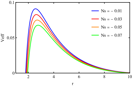
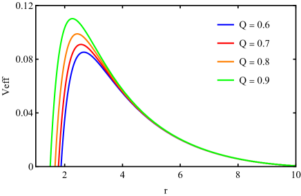
(a)                                                                                         (b)

Figure 1: The effective potential of the scalar field. (a) is the effective potential for different values of $N_{s}$ and constant $Q$ and (b) is the effective potential for different values of $Q$ and constant $N_{s}$

The Fig.1 illustrates a notable trend caused by $N_{s}$ and $Q$ parameters as in the right hand side (a) for $N_{s}<0$, when $|N_{s}|$ increases, the maximum value of the effective potential decreases. On the other hand, the left panel (b) shows the maximum effective potential increases by increasing $Q$. As shown in the Fig. 1, parameters $Q$ and $N_{s}$ play a significant role in the shape of effective potential which affects the quasinormal modes for different values. In the next section, we would like to investigate the impact of these parameters on the quasinormal modes.

IV Quasinormal modes with WKB method

Different methods are applied for the calculation of quasinormal modes mash ; heidari ; leaver . In this section, we apply the WKB method for our to obtain the quasinormal mode frequencies. In the 6th order WKB method, quasinormal modes can be evaluated with the following formula Iyer ; konoplya1 ; Kono2003

$$\frac{{i(\omega_{n}^{2}-V_{0})}}{{\sqrt{-2V^{\prime\prime}_{0}}}}+\sum\limits_{j=2}^{6}{{\Omega_{j}}=n+\frac{1}{2}}$$ (21)

Note that $V_{0}$ and $V^{\prime\prime}_{0}$ represent the height of the effective potential and the second derivative with respect to the tortoise coordinate of the potential at the maxi, respectively. The $\Omega_{j}$ are the correction terms which depend on the values of the potential and higher derivatives of it at the maxi according to Kono2003 .
The results of the quasinormal modes for the scalar perturbations are given in the Tables. 1 - 2.
From Table.1 we can see that for the constant value of $N_{s}$ by increasing $Q$, the real part of quasinormal modes for $l=0,1,2$ and monopoles $(n<l)$ increase which indicates the propagating frequency, increases. However, the imaginary part for $l=0$ and $l=1$ or $2$ represents the damping timescale for the black hole and it does not have a particular behaviour for $l=0,1$ and $l=2$ in this range.

Table 1: Quasinormal modes of scalar field for $l=1$, $M=1$, $\Lambda=0.02$, $\beta=0.02$, $N_{s}=-0.01$ and various values of $Q$

		$Q=0.7$	$Q=0.8$	$Q=0.9$
$l=0$	$n=0$	$0.1374003-0.144455i$	$0.1404071-0.143539i$	$0.144138-0.142484i$
$l=1$	$n=0$	$0.287868\,-0.10491i$	$0.300852\,-0.104476i$	$0.318782\,-0.102695i$
$l=1$	$n=1$	$0.300689-0.311105i$	$0.312462-0.310839i$	$0.328737-0.307407i$
$l=2$	$n=0$	$0.474914\,-0.0943035i$	$0.496649\,-0.0944301i$	$0.52696\,-0.0933422i$
$l=2$	$n=1$	$0.473121\,-0.288294i$	$0.494497\,-0.288429i$	$0.524276\,-0.285016i$
$l=2$	$n=2$	$0.478164\,-0.489643i$	$0.498446\,-0.489825i$	$0.526908\,-0.484446i$

In Table.2 the quasinormal mode is represented for the constant value of $Q$ and different values of $N_{s}$.When the value of parameter $N_{s}$ decreases, the real part of quasinormal modes exhibits a decrease for $l=0,1,2$ and their monopoles. About the imaginary part of quasinormal modes when $N_{s}$ takes the lower value, the imaginary part turns out to be smaller and therefore lower damping timescale.

Table 2: Quasinormal modes of scalar filed for $l=1$, $M=1$, $\Lambda=0.02$, $\beta=0.02$, $Q=0.6$ and various values of $N_{s}$

		$N_{s}=-0.01$	$N_{s}=-0.03$	$N_{s}=-0.05$
$l=0$	$n=0$	$0.1349252-0.1448015i$	$0.1272706-0.1375433i$	$0.1197197-0.1303769i$
$l=1$	$n=0$	$0.2781200-0.1048082i$	$0.2655281-0.0991626i$	$0.2530085-0.09360868i$
$l=1$	$n=1$	$0.2918233-0.310067i$	$0.2782748-0.2934625i$	$0.2648249-0.2771083i$
$l=2$	$n=0$	$0.4586723-0.09379433i$	$0.4388781-0.0888133i$	$0.419147-0.08390988i$
$l=2$	$n=1$	$0.4571753-0.286934i$	$0.43742-0.2716034i$	$0.4177378-0.25651i$
$l=2$	$n=2$	$0.4630524-0.4873898i$	$0.4427628-0.4612892i$	$0.4225712-0.4355807i$

     

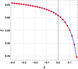
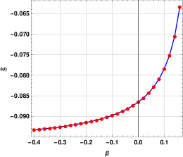
Figure 2: Variation of quasinormal modes with $M=1$, $n=0,l=3,N_{s}=-0.01,Q=0.3$ and $\Lambda=0.02$ for massless scalar perturbation.

     

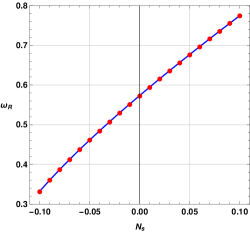
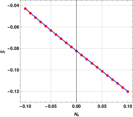
Figure 3: Variation of quasinormal modes with $M=1$, $n=0,l=3,\beta=0.01,Q=0.3$ and $\Lambda=0.02$ for massless scalar perturbation.

     

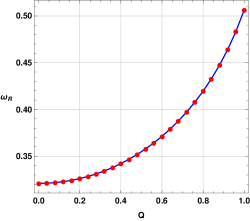
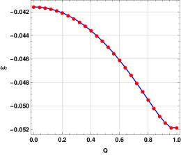
Figure 4: Variation of quasinormal modes with $M=1$, $n=0,l=3,N_{s}=-0.1,\beta=0.1$ and $\Lambda=0.02$ for massless scalar perturbation.

To have a better realisation of the quasinormal mode dependency on the model parameters of the black hole, we have plotted the real and imaginary quasinormal modes with respect to the model parameters. In Fig. 2, we have shown the variation of real and imaginary quasinormal modes with respect to the Rastall parameter $\beta$. One can see that $\beta$ impacts the oscillation frequencies of ring-down GWs non-linearly. With an increase in $\beta$, oscillation frequency decreases drastically. The decay or damping rate of GWs also decreases non-linearly with an increase in the value of $\beta$. It seems that the violation of energy-momentum conservation can have significant impacts on ring-down GWs.

In the Fig. 3, we have shown the variation of quasinormal modes with respect to the black hole structural parameter $N_{s}$. It is important to the fact that the value of $N_{s}$ is closely associated with weak energy condition. For positive values of $N_{s}$, the weak energy condition is violated. In such a scenario, both the oscillation frequency of ring - down GWs or real quasinormal modes and damping rate increases significantly.

Finally, in Fig. 4, we have shown the impacts of black hole charge on the quasinormal modes. It is seen that an increase in $Q$, increases the real part of quasinormal modes non-linearly. In the case of damping rate also, we observe a non-linear increase of the damping rate with an increase in the value of $Q$. However, near $Q=1$, a slight reverse pattern is observed. Our investigation suggests that recent observational constraints on Rastall gravity Tang can have significant impacts on the quasinormal mode spectrum. In the near future, utilising observational results from LISA, we can have a constraint on the theory from GWs and then it might be possible to check whether constraints put by Ref. Tang stands in agreement with this.

V Evolution of Scalar Perturbations on the Black hole geometry

In the preceding section of our investigation, our primary focus was on the numerical computation of the quasinormal modes and their behaviour in relation to the model parameters such as black hole charge, structural constant and Rastall parameter. Now, our attention turns to the examination of the time domain profiles of scalar perturbations. This analysis necessitates the utilization of a highly effective technique called the time domain integration formalism, which was originally introduced by Gundlach gundlach .

To commence our exploration, we establish the scalar field as $\psi(r^{*},t)=\psi(i\Delta r^{*},j\Delta t)=\psi_{i,j}$, where $r^{*}$ represents the tortoise coordinate and $t$ denotes time. Correspondingly, we define the potential as $V(r(r^{*}))=V(r^{*},t)=V_{i,j}$. By incorporating these definitions, we are able to express the governing equation of the scalar field in a discretized form:

$$\dfrac{\psi_{i+1,j}-2\psi_{i,j}+\psi_{i-1,j}}{\Delta r^{*2}}-\dfrac{\psi_{i,j+1}-2\psi_{i,j}+\psi_{i,j-1}}{\Delta t^{2}}-V_{i}\psi_{i,j}=0.$$ (22)

To initiate the temporal evolution of the scalar field, we establish the following initial conditions: $\psi(r^{*},t)=\exp\left[-\dfrac{(r^{*}-k_{1})^{2}}{2\sigma^{2}}\right]$, representing a Gaussian wave-packet, and $\psi(r^{*},t)|_{t<0}=0$. In this context, $k_{1}$ and $\sigma$ correspond to the median and width of the initial wave packet, respectively.

By employing an iterative scheme, we can compute the time evolution of the scalar field employing as follows:

$$\psi_{i,j+1}=-\,\psi_{i,j-1}+\left(\dfrac{\Delta t}{\Delta r^{*}}\right)^{2}(\psi_{i+1,j+\psi_{i-1,j}})+\left(2-2\left(\dfrac{\Delta t}{\Delta r^{*}}\right)^{2}-V_{i}\Delta t^{2}\right)\psi_{i,j}.$$ (23)

To obtain the profile of $\psi$ with respect to time $t$, we apply the aforementioned iterative scheme. It is crucial to note that throughout the numerical procedure, we must select a fixed value for the ratio $\frac{\Delta t}{\Delta r^{*}}$ and ensure that it remains less than 1. This restriction guarantees the satisfaction of the Von Neumann stability condition, thereby preserving the numerical stability of our calculations.

Through the implementation of the time domain integration formalism described above, we can gain valuable insights into the temporal characteristics of scalar perturbations. This enables us to obtain a comprehensive understanding of the dynamic behaviour exhibited by the system under investigation.

     

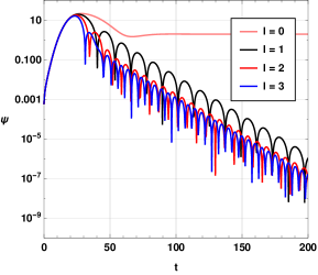
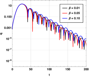
Figure 5: Time domain profiles with $M=1$, $n=0,Q=0.3$ and $\Lambda=0.02$ for massless scalar perturbation. We have used $\beta=0.05$ and $N_{s}=0.01$ on the first panel and $l=1$ and $N_{s}=-0.01$ on the second panel.

     

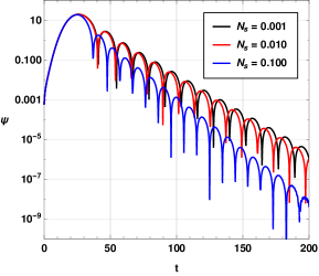
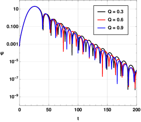
Figure 6: Time domain profiles with $M=1$, $n=0$, $l=1$, $\beta=0.05$ and $\Lambda=0.02$ for massless scalar perturbation. We have used $Q=0.3$ on the first panel and $N_{s}=0.01$ on the second panel.

We have shown the time evolution profiles for massless scalar perturbation for different values of multipole moment $l$ on the first panel of Fig. 5. One can see that with an increase in the value of multipole moment $l$, the decay rate or damping rate as well as the oscillation frequency of ring-down GWs increases. For $l=0$, one may note that the perturbation is unstable and corresponds to a positive value of imaginary quasinormal mode as seen from the previous results.

The impact of energy-momentum conservation violation is shown on the second panel of Fig. 5. The time domain profiles depict a significant impact of the Rastall parameter $\beta$ on the time domain profiles of scalar perturbation. Similarly, we have shown the impacts of black hole structural parameter $N_{s}$ and charge $Q$ on the time domain profiles on the first and second panels of Fig. 6 respectively. These results show that the black hole hairs or the model parameters can have different impacts on the time domain profiles and quasinormal mode spectrum. In the near future, with observational results from space-based GW detectors like LISA, it might be possible to constrain such theories effectively. Moreover, the detection of ring-down GWs can also shed some light on the possibility of energy-momentum conservation violation.

VI Scattering and Greybody factor

In this section, we investigate the scattering process using the WKB method. The absorption cross-section is another an important aspect of gravitational perturbations around a black hole spacetime. the probability for an outgoing wave to reach infinity or the probability for an incoming wave to be absorbed by the black hole is defined as greybody factor konoplya3 ; cardoso ; dey which plays an important role in studying the tunnelling probability of the field through the effective potential of the given black hole spacetime. We have shown the effective potential in Fig. 1, which demonstrates the effect of $N_{s}$ and $Q$ on the $V_{eff}$. Therefore, the influence of these parameters on the greybody factor and absorption cross-section are in our interest.
Scattering via the WKB method requires boundary conditions as the filed near the horizon and at infinity are expected to have these asymptotic form cardoso2

$$R_{\omega l}=\begin{cases}{{e^{-i\omega{r^{*}}}}+R{e^{i\omega{r^{*}}}}}\quad if\ {r^{*}}\to-\infty~{}(r\to{r_{h}})\\ {T{e^{-i\omega{r^{*}}}}}\quad\quad\quad\quad if\ {r^{*}}\to+\infty~{}(r\to\infty)\\ \end{cases}$$ (24)

where $R$ and $T$ are the reflection and transmission coefficients, respectively. These coefficients can be obtained by

$$|R|^{2}=\frac{1}{1+e^{-2i\pi\mathcal{K}}},$$ (25)

$$|T|^{2}=\frac{1}{1+e^{+2i\pi\mathcal{K}}}=1-|R|^{2}$$ (26)

$\mathcal{K}$ is a parameter which can be determined by following equation Kono2003

$$\mathcal{K}=\frac{i({\omega}^{2}-V_{0})}{\sqrt{-2V^{\prime\prime}_{0}}}-\sum_{j=2}^{6}\Omega_{j}$$ (27)

here $V_{0}$ is the maximum of the effective potential, $V^{\prime\prime}_{0}$ is the the second derivative of the effective potential in its maximum with respect to the tortoise coordinate $r^{*}$, and $\Omega$ are higher order WKB corrections which depend on derivatives of the effective potential at its maximumshutz ; devi ; Iyer .
Now, the grey body factor for each multipole number is calculated. We represent the greybody factor of the scalar field with respect to $\omega$. The left panel of Fig.7, (a), illustrates that increasing the value of $N_{s}$ leads to a decrease in the grey-body factors, indicating a smaller fraction of the scalar field is penetrating the potential barrier. The right panel of Fig.7, (b), shows increasing the value of $Q$ has the same impact on the greybody factor as increasing $N_{s}$. Therefore these results are consistent with the investigation of effective potential in Fig.1 that when for a constant $Q$ value, the $N_{s}$ increases or in the situation of constant $N_{s}$, $Q$ increases, the height of the effective potential barrier goes higher which means that a smaller fraction of the scalar field is penetrating the potential barrier or the probability for an outgoing wave to reach infinity called greybody factor decreased. On the other hand, when the value of $\beta$ goes higher from $0.04$ to $0.16$, the greybody factor experiences a higher value and shifts leftward.

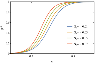
(a)

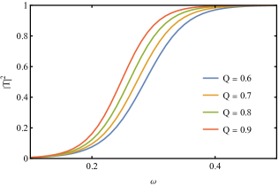
(b)

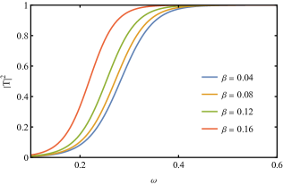
(c)

Figure 7: The greybody factors of the scalar field are computed using the third-order WKB method for $M=1$ and $l=1$. The left panel shows the results for $Q=0.7$, $\beta=0.02$ and $N_{s}=-0.01,-0.03,-0.05$ and$-0.07$, while the middle panel represents the results for $N_{s}=-0.01$ , $\beta=0.02$ and $Q=0.6,0.7,0.8$ and $0.9$ and the left panel shows the grey body factor for constant $Q=0.7$, $N_{s}=-0.01$ and variation of $\beta$

VII Concluding Remarks

In this work, we have investigated the quasinormal modes, scattering and greybody factors of AdS/dS Reissner-Nordström black hole surrounded by quintessence field in Rastall gravity. We have found that the black hole structural constant as well as charge have noticeable impacts on the quasinormal mode spectrum of the black hole. It is observed that for $l=0$ and $n=0$, one can have unstable modes with a positive imaginary quasinormal modes corresponding to a smaller value of black hole charge $Q$. However, for a higher black hole charge, the black hole spacetime becomes stable emitting physical quasinormal modes. It is seen from the Eq. (15) that for smaller values of $\beta$, a positive structural constant $N_{s}$ results in violation of the weak energy condition which can be avoided by considering large values of $\beta$ or negative values of $\beta$. Since large values of $\beta$ may give rise to unstable quasinormal modes, we chose negative $N_{s}$ values to get weak energy condition respecting scenario. Our investigation shows that $N_{s}$ has a linear impact on the quasinormal modes of the black hole and for negative $N_{s}$ values, both real quasinormal modes and damping rates are smaller. Rastall parameter $\beta$ and black hole charge $Q$ are found to have non-linear impacts on the quasinormal modes.

In the case of greybody factors, we observe that both $N_{s}$ and $Q$ have similar types of impacts on the greybody factors. By the conditions mentioned for 7, increasing $Q$ for the constant condition of other values leads to a higher greybody factor and also a higher absolute value of $N_{s}$ with other constant parameters results in increasing of greybody factor, but $\beta$ has opposite influence and when $\beta$ increases, greybody factor goes down.

In conclusion, our investigation of the quasinormal modes, scattering, and greybody factors of the AdS/dS Reissner-Nordström black hole surrounded by a quintessence field in Rastall gravity has revealed the significant impacts of the black hole structural constant and charge on the quasinormal mode spectrum, emphasizing stability and physical emission. We have also found that the Rastall parameter and black hole charge have non-linear effects on the quasinormal modes, while the black hole structural constant and charge exhibit similar trends in their influence on the greybody factors. Incorporating recent observational constraints on Rastall gravity Tang and future data from LISA, we anticipate obtaining further constraints on the theory through GWs, allowing us to assess the agreement between the imposed constraints and emerging evidence, thereby enhancing our understanding of Rastall gravity’s compatibility with observational data.

References

- (1) C. M. Will, The Confrontation between General Relativity and Experiment, Living Rev. Relativ. 17, 4 (2014).
- (2) R. A. Hulse and J. H. Taylor, Discovery of a Pulsar in a Binary System, The Astrophysical Journal Letters 195, L51 (1975).
- (3) T. Damour and J. H. Taylor, Strong-Field Tests of Relativistic Gravity and Binary Pulsars, Phys. Rev. D 45, 1840 (1992).
- (4) D. Liang, Y. Gong, S. Hou and Y. Liu, Polarizations of Gravitational Waves in Gravity, Phys. Rev. D 95, 104034 (2017).
- (5) D. J. Gogoi and U. D. Goswami, A New f(R) Gravity Model and Properties of Gravitational Waves in It, Eur. Phys. J. C 80, 1101 (2020).
- (6) D. J. Gogoi and U. D. Goswami, Gravitational Waves in Gravity Power Law Model, Indian J Phys (2021) [arXiv:1901.11277].
- (7) M. Visser, Rastall Gravity Is Equivalent to Einstein Gravity, Phys. Lett. B 782, 83 (2018)[arXiv:1711.11500].
- (8) F. Darabi, H. Moradpour, I. Licata, Y. Heydarzade, and C. Corda, Einstein and Rastall Theories of Gravitation in Comparison, Eur. Phys. J. C 78, 25 (2018).
- (9) V. Ferrari and L. Gualtieri, Quasi-Normal Modes and Gravitational Wave Astronomy, Gen. Relativ. Gravit. 40, 945 (2008).
- (10) C. V. Vishveshwara, Stability of the Schwarzschild Metric, Phys. Rev. D 1, 2870 (1970).
- (11) W. H. Press, Long Wave Trains of Gravitational Waves from a Vibrating Black Hole, ApJ 170, L105 (1971).
- (12) S. Chandrasekhar and S. Detweiler, The Quasi-Normal Modes of the Schwarzschild Black Hole, Proc. R. Soc. Lond. A 344, 441 (1975).
- (13) R. A. Konoplya, Quasinormal Behavior of the D -Dimensional Schwarzschild Black Hole and the Higher Order WKB Approach, Phys. Rev. D 68, 024018 (2003).
- (14) A. M. Oliveira, H. E. S. Velten, J. C. Fabris and L. Casarini, Neutron Stars in Rastall Gravity, Phys. Rev. D 92, 044020 (2015).
- (15) J. Bora, D. J. Gogoi, S. K. Maurya, and G. Mustafa, Impact of Energy-Momentum Conservation Violation on the Configuration of Compact Stars and Their GW Echoes, preprint, arXiv:2306.01024 (2023).
- (16) Y. Heydarzade, H. Moradpour, and F. Darabi, Black Hole Solutions in Rastall Theory, Can. J. Phys. 95, 1253 (2017).
- (17) Y. Heydarzade and F. Darabi, Black Hole Solutions Surrounded by Perfect Fluid in Rastall Theory, Physics Letters B 771, 365 (2017).
- (18) S. Chen, J. Jing, Quasinormal modes of a black hole surrounded by quintessence Class. Quantum Gravity 22, 4651 (2005).
- (19) Y. Zhang, Y.X. Gui, Quasinormal modes of a Schwarzschild black hole surrounded by quintessence, Class. Quantum Gravity 23, 6141 (2006).
- (20) Y. Zhang, Y.X. Gui, F. Li, Quasinormal modes of a Schwarzschild black hole surrounded by quintessence: electromagnetic perturbations, Gen. Relativ. Gravit. 39, 1003 (2007).
- (21) C. Ma, Y. Gui, W. Wang, F. Wang, Massive scalar field quasinormal modes of a Schwarzschild black hole surrounded by quintessence, Cent. Eur. J. Phys. 6, 194 (2008).
- (22) Y. Zhang, Y.X. Gui, F. Yu, Dirac quasinormal modes of a Schwarzschild black hole surrounded by free static spherically symmetric quintessence, Chin. Phys. Lett. 26, 030401 (2009).
- (23) J. P. M. Graça and I. P. Lobo, Scalar QNMs for Higher Dimensional Black Holes Surrounded by Quintessence in Rastall Gravity, Eur. Phys. J. C 78, 101 (2018).
- (24) J. Liang, Quasinormal Modes of the Schwarzschild Black Hole Surrounded by the Quintessence Field in Rastall Gravity, Commun. Theor. Phys. 70, 695 (2018).
- (25) Y. Hu, C.-Y. Shao, Y.-J. Tan, C.-G. Shao, K. Lin, and W.-L. Qian, Scalar Quasinormal Modes of Nonlinear Charged Black Holes in Rastall Gravity, EPL 128, 50006 (2020).
- (26) Z. Xu, X. Hou, X. Gong, and J. Wang, Kerr–Newman-AdS Black Hole Surrounded by Perfect Fluid Matter in Rastall Gravity, Eur. Phys. J. C 78, 513 (2018).
- (27) K. Lin and W.-L. Qian, Neutral Regular Black Hole Solution in Generalized Rastall Gravity, Chinese Phys. C 43, 083106 (2019).
- (28) D. J. Gogoi, R. Karmakar, and U. D. Goswami, Quasinormal Modes of Non-Linearly Charged Black Holes Surrounded by a Cloud of Strings in Rastall Gravity, arXiv:2111.00854 (2021).
- (29) D. J. Gogoi and U. D. Goswami, Quasinormal Modes of Black Holes with Non-Linear-Electrodynamic Sources in Rastall Gravity, Physics of the Dark Universe 33, 100860 (2021) [arXiv:2104.13115].
- (30) D. J. Gogoi, A. Övgün, and D. Demir, Quasinormal Modes and Greybody Factors of Symmergent Black Hole, preprint, arXiv:2306.09231 (2023).
- (31) Y. Sekhmani and D. J. Gogoi, Electromagnetic Quasinormal Modes of Dyonic AdS Black Holes with Quasitopological Electromagnetism in a Horndeski Gravity Theory Mimicking EGB Gravity at , Int. J. Geom. Methods Mod. Phys. 2350160 (2023) [arXiv:2306.02919].
- (32) G. Lambiase, R. C. Pantig, D. J. Gogoi, and A. Övgün, Investigating the Connection between Generalized Uncertainty Principle and Asymptotically Safe Gravity in Black Hole Signatures through Shadow and Quasinormal Modes, preprint, arXiv:2304.00183 (2023).
- (33) D. J. Gogoi, A. Övgün, and M. Koussour, Quasinormal Modes of Black Holes in Gravity, preprint, arXiv:2303.07424 (2023)
- (34) D. J. Gogoi and U. D. Goswami, Tideless Traversable Wormholes surrounded by cloud of strings in f(R) gravity, JCAP 02, 027 (2023).
- (35) R. Karmakar, D. J. Gogoi and U. D. Goswami, Quasinormal modes and thermodynamic properties of GUP-corrected Schwarzschild black hole surrounded by quintessence, IJMP A 37, 28 (2022).
- (36) D. J. Gogoi and U. D. Goswami, Quasinormal Modes and Hawking Radiation Sparsity of GUP Corrected Black Holes in Bumblebee Gravity with Topological Defects, JCAP 06, 029 (2022).
- (37) A. Övgün, İ. Sakallı and J. Saavedra, Quasinormal Modes of a Schwarzschild Black Hole Immersed in an Electromagnetic Universe, Chin. Phys. C 42, no.10, 105102 (2018) arXiv:1708.08331[physics.gen-ph]].
- (38) A. Övgün, İ. Sakallı and H. Mutuk, Quasinormal modes of dS and AdS black holes: Feedforward neural network method, Int. J. Geom. Meth. Mod. Phys. 18, no.10, 2150154 (2021) [arXiv:1904.09509 [gr-qc]].
- (39) D. J. Gogoi, Y. Sekhmani, D. Kalita, N. J. Gogoi, and J. Bora, Joule‐Thomson Expansion and Optical Behaviour of Reissner‐Nordström‐Anti‐de Sitter Black Holes in Rastall Gravity Surrounded by a Quintessence Field, Fortschritte Der Physik 71, 2300010 (2023) [arXiv:2306.02881].
- (40) C. Gundlach, R. H. Price and J. Pullin, Late time behavior of stellar collapse and explosions: 2. Nonlinear evolution, Phys. Rev. D 49, 890 (1994) [arXiv:gr-qc/9307010].
- (41) M. Tang, Z. Xu, and J. Wang, Observational Constraints on Rastall Gravity from Rotation Curves of Low Surface Brightness Galaxies, Chinese Phys. C 44, 085104 (2020).
- (42) V. Ferrari, and B. Mashhoon, New approach to the quasinormal modes of a black hole, Physical Review D 30, no. 2 (1984): 295.
- (43) N. Heidari, and H. Hassanabadi, Investigation of the quasinormal modes of a Schwarzschild black hole by a new generalized approach, Physics Letters B 839 (2023): 137814.
- (44) Leaver, Edward W. Quasinormal modes of Reissner-Nordström black holes, Physical Review D 41, no. 10 (1990): 2986.
- (45) S. Devi, R. Roy, and S. Chakrabarti, Quasinormal modes and greybody factors of the novel four dimensional Gauss–Bonnet black holes in asymptotically de Sitter space time: scalar, electromagnetic and Dirac perturbations, The European Physical Journal C 80, no. 8 (2020): 760.
- (46) B. F. Schutz and Clifford M. Will, Black hole normal modes: a semi analytic approach, The Astrophysical Journal 291 (1985): L33-L36.
- (47) S. Iyer, and Clifford M. Will. Black-hole normal modes: A WKB approach. I. Foundations and application of a higher-order WKB analysis of potential-barrier scattering, Phys. Rev. D 35, no. 12 (1987): 3621.
- (48) R. A. Konoplya, Quasinormal modes of a small Schwarzschild–anti-de Sitter black hole, Phys. Rev. D 66, no. 4 (2002): 044009.
- (49) R. A. Konoplya and A. F. Zinhailo Hawking radiation of non-Schwarzschild black holes in higher derivative gravity: a crucial role of grey-body factors, Phys. Rev. D 99, no. 10 (2019): 104060.
- (50) V. Cardoso, M. Cavaglia, and L. Gualtieri, Black hole particle emission in higher-dimensional spacetimes, Phys. Rev. Lett. 96, no. 7 (2006): 071301.
- (51) S. Dey, and S. Chakrabarti, A note on electromagnetic and gravitational perturbations of the Bardeen de Sitter black hole: quasinormal modes and greybody factors, The European Physical Journal C 79, no. 6 (2019): 504.
- (52) V. Cardoso and J. PS Lemos, Quasinormal modes of Schwarzschild–anti-de Sitter black holes: Electromagnetic and gravitational perturbations, Phys. Rev. D 64, no. 8 (2001): 084017.