Scale-dependent analysis of angular momentum flux in high-resolution magnetohydrodynamic simulations for solar differential rotation
Abstract
In this work, we systematically investigate the scale-dependent angular momentum flux by analysing high-resolution three-dimensional magnetohydrodynamic simulations in which the solar-like differential rotation is reproduced without using any manipulations. More specifically, the magnetic angular momentum transport (AMT) plays a dominant role in the calculations. We examine the important spatial scales for the magnetic AMT. The main conclusions of our approach can be summarized as follows: 1. Turbulence transports the angular momentum radially inward. This effect is more pronounced in the highest resolution calculation. 2. The dominant scale for the magnetic AMT is the smallest spatial scale. 3. The dimensionless magnetic correlation is low in the high-resolution simulation. Thus, chaotic but strong small-scale magnetic fields achieve efficient magnetic AMT.
keywords:
Sun: interior – Sun: rotation1 Introduction
The Sun’s differential rotation (DR) is a crucial process for generating its magnetic field through the effect (Parker, 1955). The existence of the DR effect was experimentally demonstrated in the early 1630s by tracking sunspots (Paternò, 2010). In the modern era, helioseismology has revealed the detailed profile of the DR (e.g., Schou et al., 1998). The fast equator is considered to be the most prominent feature of the solar DR. In particular, the solar equator rotates in a 25-day period, while the polar region rotates in a 30-day period.
From a theoretical (numerical) viewpoint, solar-like DR, where the equator rotates faster than the polar regions, can be reproduced with a low Rossby number (Ro) (i.e. strong rotational influence), where the Ro is defined with , , and refer to the typical convection velocity, the system rotation rate, and the typical convection spatial scale, respectively. When the system is located in a high-Ro regime (i.e. weak rotational influence), the polar region starts to rotate faster, which is called the anti-solar DR (e.g., Gastine et al., 2014). There is a consensus in the scientific community that the Sun lies in the low-Ro regime because it has a solar-like DR. However, the convective conundrum related to solar angular momentum transport (AMT) has raised questions about the former assumption. Alarmingly, high-resolution simulations, even those including solar parameters, such as solar rotation rate and luminosity, can easily fail to simulate the solar-like DR (Hotta et al., 2015; O’Mara et al., 2016). Moreover, the high-resolution simulation tends to generate a high-Ro regime, which accelerates the polar region (see Mori & Hotta, 2023, hereafter MH23)
Recently, Hotta & Kusano (2021) (hereafter HK21) solved this problem. When the resolution was increased to unprecedentedly high levels, the magnetic energy exceeded the kinetic energy. As a result, the Maxwell stress can transport the angular momentum and lead to a fast equator (see also Hotta et al., 2022, hereafter HKS22). According to the literature, the equatorial acceleration can be achieved by outward AMT from the rotational axis with rotationally constrained turbulence (Karak et al., 2015; Käpylä, 2022, MH23). In their high-resolution simulation, however, HKS22 found that the magnetic field is the dominant component of the AMT. Even though the scale analysis by HKS22 implies that small-scale magnetic fields can be the dominant aspect of AMT, HKS22 did not decompose the angular momentum flux (AMF) into separate scales. Thus, HKS22 did not identify any direct evidence for the importance of the small-scale magnetic fields in the AMT. Thus we analyse the HK21 calculation results using the spatial scale decomposition method for the AMF suggested in MH23. We address three main issues in this work:
-
A.
What is the most important scale of the magnetic field for accelerating the equator?
-
B.
Does the inward AMT by the turbulence become stronger at smaller scales?
-
C.
Is the magnetic field important because the magnetic field is strong or because the magnetic fields are correlated?
We thoroughly investigate the importance of the small-scale magnetic field for the AMT using the above scale decomposition (Issue A). MH23 suggested that the smaller scale turbulence has stronger radially inward AMT with a weaker rotational influence. We can confirm this pattern by analysing high-resolution simulations (Issue B). HKS22 found also that the magnetic AMT is dominant in their high-resolution calculation. Since the momentum flux is a form of covariance , the strong magnetic AMT can be interpreted by considering two possibilities. The first one is related to the fact that just the magnetic field strength is high. MH21 already reported that the magnetic field is significantly strong in their calculation, which could explain this effect. The other possibility is that the dimensionless correlation is high. In particular, HKS22 found that the correlation between the magnetic fields is generated by high-Ro turbulence. Typically, turbulence on a smaller scale is less affected by the rotational influence; that is, the higher Ro. Thus, smaller-scale magnetic fields may be more strongly correlated than larger-scale magnetic fields (Issue C).
This manuscript is constructed as follows. We describe the model setup for the numerical simulations in Section 2. We present the proposed method to decompose the AMT in Section 3. Next, we thoroughly discuss the results of our analysis in Section 4. The scale decomposition of the AMF and the correlation are also shown in Section 4. Finally, we summarize and conclude the paper in Section 5.
2 Numerical Model
We explain our developed numerical model setup in this section. We analyse the results of the HK21 calculations, which provide three different resolution calculations: namely, Low, Middle, and High (see Table 1).
| Case | No. of Grid points |
|---|---|
| Low | |
| Middle | |
| High |
HKS22 supplied dimensionless quantities for the calculations (see their Table 1). We convert the Yin–Yang grid (Kageyama & Sato, 2004) into spherical geometry for analyses. The radial extent of the computational domain is , where is the solar radius. We use the R2D2 (Radiation and RSST for Deep Dynamics) code (Hotta et al., 2019; Hotta & Iijima, 2020; Hotta & Kusano, 2021), where RSST represents the reduced speed of sound technique (Hotta et al., 2012). We use Model S (Christensen-Dalsgaard et al., 1996) for the background stratification and related variables. We also use the solar luminosity and solar rotation rate (see HKS22 for more details). The calculation continues for days for each case and the following results are averaged between to days unless otherwise noted.
3 Decomposition method
In this work, we decompose the Reynolds (flow) and Maxwell (magnetic) AMFs111The AMF caused by the Reynolds (Maxwell) stress is called the “Reynolds (Maxwell) AMF” in this study. to scale-dependent values using the Fourier transforms in the longitudinal direction. MH23 suggested using the spatial scale decomposition method. The Reynolds and Maxwell AMFs are written as follows:
| (1) |
where or , , and is the fluid velocity in the rotating frame. The parenthesis denotes the longitudinal average. ′ represents perturbations from the longitudinal average, such as . We decompose these AMFs using Parseval’s theorem as follows:
| (2) |
The mean magnetic field is weak compared with the perturbation ; therefore, we exclude the contribution by the . We do not decompose the scale based on the wavenumber , but on the actual spatial scale (see MH23, particularly eqs (17)–(20) and Table 1). The scale-dependent AMF can be defined as follows:
| (3) |
where refers to the Fourier transform in the longitudinal direction defined by MH23 (see their eq. (12)) and ∗ indicates the complex conjugate. When , the expression becomes:
| (4) |
where is the number of grid points in the longitudinal direction. and are calculated based on the maximum and minimum scale length for the scale-dependent AMF and as:
| (5) | ||||
| (6) |
where is the floor function. and in this study is presented in Table 2, which is the same as that in MH23.
| 1 | 240 Mm | |
|---|---|---|
| 2 | 120 Mm | 240 Mm |
| 3 | 60 Mm | 120 Mm |
| 4 | 60 Mm |
Our definition of the scale-dependent AMF covers the scales (see MH23 for more details). We also define the dimensionless correlation as follows:
| (7) |
where is the root-mean-square (RMS) in the longitudinal direction. and are useful because they demonstrate the dominant contribution of the AMF, that is, the dimensionless correlations or the amplitude of the physical quantity. We also define the dimensionless scale-dependent correlation and as follows:
| (8) |
When , the expressions become
4 RESULTS
4.1 General properties
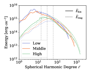
Fig. 1 shows the kinetic and magnetic energy spectra (see eqs (16) and (17) of HKS22 for the definition). The blue, orange, and green lines show the results from the Low, Middle, and High cases, respectively. As shown in HK21, the large-scale kinetic energy () is significantly reduced in the High case, whereas the magnetic energy increases as resolution becomes higher in all scales.
See Fig. 10 in HKS22 for the DR and the meridional flow. The Low case has anti-solar DR, whereas the High case possesses solar-type DR.
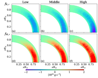
Fig. 2 shows the radial Reynolds and Maxwell AMF. Note that almost the same figure is presented by HKS22 (see their Fig. 29). Here, we review their results.
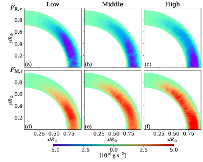
The radial AMF significantly depends on the resolution; therefore, our main focus in this work is only on the radial AMFs. The radial Reynolds AMFs are always negative (i.e., inward AMTs) and their strengths are almost the same (Figs 2a, b, and c). The radial Maxwell AMFs show positive values, that is, the outward AMT in all cases (Figs 2d, e and f). The flux strength increases as the resolution increases.
Fig. 3 shows the dimensionless velocity and magnetic correlations. We also note that is already shown in HKS22 (see their Fig. 36), but is the original result in this work.
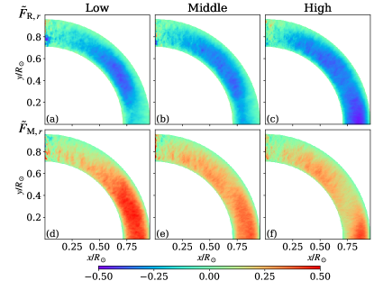
We can see the strongest negative correlation in the High case (Fig. 3c). This may be due to the high Ro in the High case (see Table 1 of HKS22 for Local Rossby number ). When the Ro is high, the downflow becomes dominant. This downflow is bent by the Coriolis force and turbulence has negative correlations (). This result indicates that makes a significant contribution to the radially inward Reynolds AMT . This strong negative correlation is thought to be caused by the high Ro due to the small-scale turbulence reproduced by the high resolution. Considering the magnetic field, the positive correlation decreases with increased resolution (Fig. 3d, e, and f). This result indicates that the strength of the magnetic field is responsible for the radially outward AMT and the resulting fast equator (Issue C in Section 1).
4.2 Scale-dependent angular momentum flux
In this subsection, we investigate the scale-dependent AMF. As explained in section 3, we decompose the AMFs into four scales (see also Table 2). We note that the index of and does not represent the wavenumber (see Section 3 for details).
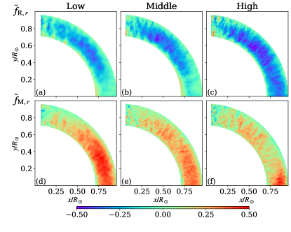
Fig. 4 shows the and , which correspond to the spatial scale of , that is, the largest scale.
We use the same colour scale in Fig. 4 and the following two figures for comparison. We extract negative Reynolds AMFs in all cases (Fig. 4a, b, and c). We find that the inward Reynolds transport is largest in the Low case because of its larger convection velocity (Fig. 1). The Maxwell AMFs are positive in all cases (Fig. 4d, e, and f). The outward transport is largest in the High case and the magnetic field strength is highest in the High case, which probably leads to the strong outward AMT (see Fig. 1).
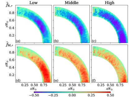
Fig. 5 shows the and the , which correspond to the spatial scale of .

Similar to , the Reynolds and Maxwell are negative and positive in all cases, respectively. We can observe the stronger Reynolds AMFs (i.e., ), especially in the Middle and High cases, while the kinetic energy is larger in (Fig. 1). We can see the similar Maxwell AMFs, i.e., in all cases.
and are almost the same as and , respectively, and are not shown here.
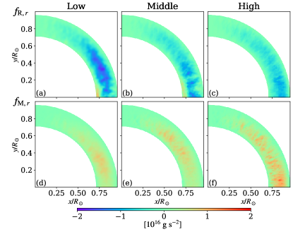
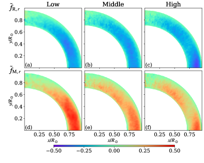
and are shown in Fig. 6. The corresponding spatial scale is , which is the smallest scale.
The Reynolds AMFs are negative in all cases. More specifically, in the High case, the inward AMT near the equator is stronger than those at other scales (Issue B in Section 1). The Maxwell AMFs are positive in all cases. We record the largest amplitude in this scale compared with the other scales, especially in the High case. Thus, we can argue that the small-scale () magnetic field is the dominant source of the AMT, as expected in HKS22 (Issue A in Section 1).
4.3 Scale-dependent dimensionless correlation
In this subsection, we use the dimensionless correlation to investigate the physical origin of the AMFs, namely, the dimensionless correlation or spectral amplitude.
Fig. 7 shows the and , which correspond to the spatial scale of .
The absolute value of the negative velocity correlation , which is related to the inward AMT, is largest in the High case. The stronger correlation is likely due to the high in the High case (see Table 1 of HKS22). The can be derived from the calculation results before the scale decomposition process. It is interesting to note that we can still see the difference between resolutions; that is, the small-scale influence in the High case, as well as the after-scale decomposition. Figs 4, and 7 illustrate that the large velocities are responsible for the large Reynolds AMF in the Low case at this scale. While the correlation is large in the High case, the small velocity amplitude leads to a small Reynolds AMF. The absolute value of positive magnetic correlation is the largest in the Low case. The higher-resolution simulation can reproduce small-scale random motions, the correlation is smaller in the High case. This effect is also in direct line with the scale-integrated AMF (Fig. 2).
Fig. 8 shows the and , which correspond to the spatial scale of .
The negative dimensionless velocity correlation is strongest in the High case and this trend also applies for . We find the absolute value of the correlation in this scale increases compared with , i.e., in all the cases. On a smaller scale, the rotational influence becomes less efficient. This pattern increases the negative velocity correlation. As far as the magnetic field is concerned, the result does not change much from scale. The dependence of the magnetic correlation on the spatial scale is smaller than that of the velocity correlation.
As for and , they are almost the same as and , respectively, which are not shown here.
The results of and are displayed in Fig. 9.
The amplitudes of the dimensionless velocity correlation are similar between the cases (Fig. 9a, b, and c). The dimensionless magnetic correlation is largest in the Low case. As the outward AMF is largest in the High case, the strength of the magnetic field is purely responsible for the strong AMT (Issue C in Section 1).
5 Summary
In this work, we systematically investigate the dependence of the AMT on the spatial scale with the method suggested by MH23. We examine three simulation results in MH21, which have different resolutions: namely, Low, Middle, and High cases. We summarize the main results of this work below:
-
1.
The absolute value of the negative dimensionless velocity correlation increases with increasing resolution, especially at the small scales.
-
2.
The outward Maxwell AMF is strongest at the smallest scale.
-
3.
The dimensionless magnetic correlation decreases with increasing resolution.
The first result indicates that the high-resolution calculation in HK21 remains in the high Ro, while the RMS velocity is reduced in the case since the small-scale turbulence is introduced. The solar-like DR is also achieved even in the high Ro regime thanks to the magnetic AMT.
The second result emphasizes the small-scale magnetic field for constructing the DR. HKS22 suggested that the magnetic AMT occurs via magnetic tension. Considering that magnetic tension is most effective on a small scale, our analysis is consistent with the results of this work.
The third result indicates that the magnetic field becomes chaotic but strong on a small scale. Although the just chaotic magnetic field cannot transport the momentum, the remaining order with high magnetic strength can transport a large amount of angular momentum. The essential role of the small-scale magnetic field on the AMT highlights the importance of a higher resolution calculation in the future.
Acknowledgements
H. Hotta. is supported by JSPS KAKENHI grants No. JP20K14510, JP21H04492, JP21H01124, JP21H04497, JP23H01210 and MEXT as a Programme for Promoting Researches on the Supercomputer Fugaku (JPMXP1020230504). The results were obtained using the Supercomputer Fugaku provided by the RIKEN Center for Computational Science (hp220173, hp230204, and hp230201).
Data Availability
The analysed data underlying this article will be shared on reasonable request to the corresponding author.
References
- Christensen-Dalsgaard et al. (1996) Christensen-Dalsgaard J., et al., 1996, Science, 272, 1286
- Gastine et al. (2014) Gastine T., Yadav R. K., Morin J., Reiners A., Wicht J., 2014, MNRAS, 438, L76
- Hotta & Iijima (2020) Hotta H., Iijima H., 2020, MNRAS, 494, 2523
- Hotta & Kusano (2021) Hotta H., Kusano K., 2021, Nature Astronomy, 5, 1100
- Hotta et al. (2012) Hotta H., Rempel M., Yokoyama T., Iida Y., Fan Y., 2012, A&A, 539, A30
- Hotta et al. (2015) Hotta H., Rempel M., Yokoyama T., 2015, ApJ, 798, 51
- Hotta et al. (2019) Hotta H., Iijima H., Kusano K., 2019, Science Advances, 5, 2307
- Hotta et al. (2022) Hotta H., Kusano K., Shimada R., 2022, ApJ, 933, 199
- Kageyama & Sato (2004) Kageyama A., Sato T., 2004, Geochemistry, Geophysics, Geosystems, 5, Q09005
- Käpylä (2022) Käpylä P. J., 2022, arXiv e-prints, p. arXiv:2207.00302
- Karak et al. (2015) Karak B. B., Käpylä P. J., Käpylä M. J., Brandenburg A., Olspert N., Pelt J., 2015, A&A, 576, A26
- Mori & Hotta (2023) Mori K., Hotta H., 2023, MNRAS, 519, 3091
- O’Mara et al. (2016) O’Mara B., Miesch M. S., Featherstone N. A., Augustson K. C., 2016, Advances in Space Research, 58, 1475
- Parker (1955) Parker E. N., 1955, ApJ, 122, 293
- Paternò (2010) Paternò L., 2010, Ap&SS, 328, 269
- Schou et al. (1998) Schou J., et al., 1998, ApJ, 505, 390