Beyond Single-Feature Importance with ICECREAM

Abstract

Which set of features was responsible for a certain output of a machine learning model? Which components caused the failure of a cloud computing application? These are just two examples of questions we are addressing in this work by Identifying Coalition-based Explanations for Common and Rare Events in Any Model (ICECREAM). Specifically, we propose an information-theoretic quantitative measure for the influence of a coalition of variables on the distribution of a target variable. This allows us to identify which set of factors is essential to obtain a certain outcome, as opposed to well-established explainability and causal contribution analysis methods which can assign contributions only to individual factors and rank them by their importance. In experiments with synthetic and real-world data, we show that ICECREAM outperforms state-of-the-art methods for explainability and root cause analysis, and achieves impressive accuracy in both tasks.

1 Introduction

Raising the question why something happened is a fundamental aspect of human nature and has always been a major driver for scientific progress across all disciplines. Moreover, answering this question is crucial to identify and resolve issues in complex systems. For instance, on-call engineers of a cloud computing application need to find out why their application is experiencing increased error rates to understand how to fix the problem and restore normal operations.

In recent years, the question “Why does the machine learning model return a certain result for a given input?” has become particularly important with the tremendous advancements of machine learning (ML) and artificial intelligence (AI) and their application in various disciplines, from life sciences and medicine all the way to political decision making (e.g. Emmert-Streib et al.,, 2020; Zhang et al.,, 2022). Understanding how black-box models work and knowing which input features most influence the model output has become a core goal in the growing field of explainability in AI (XAI) (e.g. Lundberg and Lee,, 2017; Burkart and Huber,, 2020; Gerlings et al.,, 2021). Answering this question, however, is extremely challenging since the inputs to ML models can easily be composed of hundreds or even hundreds of thousands of input features (e.g., pixels in computer vision (CV)), and the best-performing models are usually highly complex deep neural networks. Various methods have been developed to rank the importance of individual input features for the model output, ranging from gradient-based approaches (e.g. Sundararajan et al.,, 2017) to methods using Shapley values (e.g. Lundberg and Lee,, 2017; Fryer et al.,, 2021) to counterfactual reasoning (e.g. Keane and Smyth,, 2020; von Kügelgen et al.,, 2023). In many applications, however, the explanation for an event is not just the behavior of a single factor, but the combination of multiple factors that only jointly result in the observed outcome.

Identifying which coalition of factors is responsible for a given outcome provides valuable insights into the system under consideration. One such insight, for instance, is understanding which input factors need to be changed to obtain a desired change in the output. Let us take a look at two simple examples where not a single factor, but a coalition of variables is important for a certain outcome:

Example 1.

Consider a cloud computing application that is set up with redundancies to prevent errors from propagating through the system. The system only fails when multiple components experience an issue. A simple example of such a system are two binary input variables $X_{1}$ and $X_{2}$ and a binary target $Y$. The input variables independently follow Bernoulli distributions with parameters $p_{1}$ and $p_{2}$, respectively, and the target value $y$ is the deterministic AND of the inputs: $Y=X_{1}\wedge X_{2}$. The corresponding graphical model is shown in Figure 1 and all possible outcomes for this setup can be found in Table 1. As long as at least one of the two input factors is “healthy” (i.e., $X_{1}=0$ or $X_{2}=0$), the target does not experience an issue. However, if both inputs encounter an error (i.e., $X_{1}=X_{2}=1$), this leads to a failure in the target $Y$.

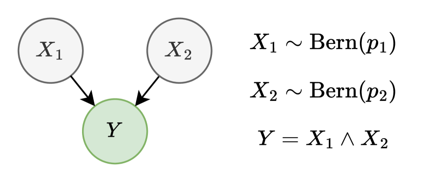
Figure 1: Graphical causal model for Example 1. The variables $X_{1}$ and $X_{2}$ independently follow Bernoulli distributions, while $Y$ is completely determined by the values of its causal parents.

Table 1: All possible outcomes for Example 1. Additionally, we provide the explanation scores from Equation 2 in Section 3 for parameter values $p_{1}=0.1$, $p_{2}=0.8$.

case 1: case 2: case 3: case 4: $x_{1}$ 0 0 1 1 $x_{2}$ 0 1 0 1 $y$ 0 0 0 1 $\mathcal{E}(\{X_{1}\})$ $1.0$ $1.0$ $-18.3$ $0.9$ $\mathcal{E}(\{X_{2}\})$ $1.0$ $-0.3$ $1.0$ $0.1$ $\mathcal{E}(\{X_{1},X_{2}\})$ $1.0$ $1.0$ $1.0$ $1.0$

Example 2.

Consider an ML model that predicts the risk of credit applications based on the South German Credit dataset which contains various input features like age, housing situation, credit amount, duration, purpose, etc. (Grömping,, 2019). For a specific application, the model predicts a high credit risk, and we would like to know why the model came to this conclusion and which features were relevant for the decision. We can use e.g. the well-established SHAP method (Lundberg and Lee,, 2017) to quantify the importance of the individual features for this particular prediction. This ranking shows that the credit purpose, housing situation, and personal status are the 3 most important features for this output. However, it does not tell us what combination of features was crucial for the outcome, and how many features are actually required to explain the target value. One possibility would be to consider a fixed number of features or or to merge them into high-level features. But as we show e.g. in Appendix B this does not resolve the problem.

In this paper, we present ICECREAM, a novel approach for Identifying Coalition-based Explanations for Common and Rare Events in Any Model. ICECREAM is designed to detect coalitions of variables whose interplay explains the observed outcome, instead of ranking single features based on their individual importance. For this we define an explanation score which uses an information-theoretic approach to measure the contribution of groups of variables, inspired by the work on optimal feature selection by Koller and Sahami, (1996). ICECREAM can be used for explainability and interpretability of any feature/target system. Moreover, by incorporating a causal notion, it can also be applied in any system with a known causal structure, e.g., to perform root cause analysis (RCA) in a cloud computing system. We provide the required background on graphical causal models in Section 2, introduce the proposed method in Section 3, discuss related work in Section 4, and present experiments with both synthetic and real-world data in Section 5. Finally, we conclude the paper in Section 6.

2 Graphical causal models

Many systems for which we want to provide explanations can be represented as graphical causal models (Pearl,, 2009). For instance, Figure 1 shows the graphical causal model corresponding to Example 1: three observed variables where $X_{1}$ and $X_{2}$ causally influence $Y$. In general, these models represent the causal relations in a system via a directed graph $G=(\bm{V},\bm{E})$ with nodes $\bm{V}=\{V_{1},...,V_{N}\}$ corresponding to random variables (RVs) $V_{i}$ with domains $\mathcal{V}_{i}$. An edge $(V_{i},V_{j})\in\bm{E}$, also represented in the graph as $V_{i}\rightarrow V_{j}$, means that $V_{i}$ has a direct causal influence on $V_{j}$.

When a variable $V_{i}$ is set to some value $v_{i}$ in a hypothetical scenario where the other variables keep their relationships intact, this is called a (hard) intervention on $V_{i}$. In the graph, such an intervention is represented by cutting all edges between $V_{i}$ and its causal parents $\bm{P\!A}_{i}$. Pearl’s do-operator formalizes the change of the joint distribution $\mathbb{P}[V_{1},\dots,V_{N}]$ that results from such an intervention and provides ways to compute the interventional distribution $\mathbb{P}[V_{j}\mid do(V_{i}=v_{i})]$ under certain conditions (Pearl,, 2009, Chapter 3.4). We use the shorter notation $\mathbb{P}[V_{j}\mid do(V_{i})]$ whenever the value $v_{i}$ of the intervention can be inferred from context.

Note that this interventional distribution must not be confused with the observational conditional distribution $\mathbb{P}[V_{j}\mid V_{i}=v_{i}]$: For example, conditional probabilities do not distinguish between the causal and anti-causal directions, while interventional probabilities do. The reason is that knowing that an effect happened also makes us update the probability of its causes, while intervening on an effect does not affect its causes at all. The interventional and conditional distributions only coincide if the variable $V_{i}$ has no causal parents.

We assume that the system under consideration can be partitioned into two sets of variables: first, a set $\bm{X}=\{X_{1},\dots,X_{n}\}$ of observed (endogenous) variables; and second, a set of unobserved (exogenous) noise variables $\bm{\Lambda}=\{\Lambda_{1},\dots,\Lambda_{m}\}$ which are jointly statistically independent, with $\bm{V}=\bm{X}\cup\bm{\Lambda}$ and $m\geq n$ such that each observed variable $X_{i}$ is causally influenced by at least one noise variable $\Lambda_{i}$. Without loss of generality, we assume that the observed variables $\bm{X}$ are in topological order in the graph $G$, i.e., $i<j$ for all $(X_{i},X_{j})\in\bm{E}$. For the remainder of this paper, we consider $X_{n}$ to be the target whose value we want to explain, and denote this variable with the alias $Y$ to distinguish it from the other variables in the system. We hereafter denote the remaining set of observed variables with $\bm{X}:=\{X_{1},\dots,X_{n-1}\}$. Further we will consider coalitions of variables, i.e., subsets of $\bm{V}$, denoted by $\bm{V}_{C}:=\{V_{i}:i\in C\}$ with $C\subseteq I:=\{1,\dots,N-1\}$. These coalitions can contain observed as well as unobserved variables from the graph. Note that we assume knowledge of the causal structure between the target $Y$ and all variables that are considered as possible explanations for the value of $Y$. However, this does not mean that we require the full causal graph of the system. For instance, if we consider the observed variables $\bm{X}$ as possible explanations of $Y$, we only need to know the causal structure among these variables and $Y$ while hidden confounders among the variables $\bm{X}$ are allowed. Admittedly, this is still a strong restriction in general, as discovering a causal graph from data is challenging and the subject of ongoing research (e.g. Spirtes et al.,, 1993; Peters et al.,, 2017). Nevertheless, as we will discuss in Section 5, for certain applications it is fair to assume the relevant causal structures to be known. Particularly, in the XAI setting the relevant graph structure is a trivial one-layer graph (cf. Janzing et al.,, 2020). Further, we assume that only interventions are possible that have a positive joint observational probability (in analogy to the positivity assumption in the potential outcomes framework (Rubin,, 2005)).

3 ICECREAM: Identifying Coalition-based Explanations for Common and Rare Events in Any Model

In this section, we present ICECREAM, a novel approach to find explanations for both common and extreme events. In contrast to established approaches for explainability and causal contribution analysis, ICECREAM is designed to handle coalitions of variables instead of ranking the importance of individual features. To achieve this, we first propose and analyze an explanation score which quantifies the influence of a set of variables on the target variable. Then we discuss how this score can be applied in practice to address the following question: What is the smallest coalition of variables which fully explains the target value $y$ for an observation $\bm{v}$?

Obviously, the set of all variables provides a full explanation for any target value in a given system. However, in order to obtain actionable insights for the system and inspired by Occam’s Razor as well as the fact that humans understand simple explanations better than complex ones, we are interested in a concise and actionable explanation, i.e., one that includes as few variables as possible.

First, we want to mention some properties we would like the explanation score used in ICECREAM to satisfy, and which are hence taken as constraints in the design of the score:

Desideratum 1.

Explanation scores of coalitions of variables should not be just the sum of the explanation scores for the individual variables.

Consider the case $x_{1}=x_{2}=y=0$ in Example 1. Here, $x_{1}=0$ alone already fully explains the target value $y=0$, and the same is true for $x_{2}=0$. Hence the coalition $\{X_{1},X_{2}\}$ should not have a higher explanation score than the two variables individually (as would be the case for additive scores).

Desideratum 2.

Rare events which are required for the considered outcome should get a higher explanation score than common events.

Consider again Example 1 and assume that $p_{1}=0.1$ and $p_{2}=0.8$. In this case, $X_{1}$ would be rarely 1, while $X_{2}$ is 1 most of the time. Intuitively—and as argued in Budhathoki et al., (2022)—, we consider $X_{1}$ to be the more interesting explanation for the outcome $y=1$. We expect this to also be reflected in the explanation score by assigning a higher score to $\{X_{1}\}$ than to $\{X_{2}\}$ in this example.

Desideratum 3.

Explanation scores in anti-causal direction should be zero.

We consider this an important property as in a causal perspective it would not make sense for the value of an effect to explain its causes. In Example 1, for instance, the explanation score of $\{Y\}$ for any value of $X_{1}$ or $X_{2}$ should always be zero since $Y$ cannot influence $X_{1}$ and $X_{2}$.

To obtain an explanation score that satisfies Desiderata 1, 3 and 2, we propose to derive the score from the change in the probability distribution of the target variable $Y$. Specifically, we consider the following three distributions: (1) the distribution $\mathbb{P}[Y\mid do(\bm{V})]$ where all variables in the system have been set to a fixed value; (2) the distribution $\mathbb{P}[Y\mid do(\bm{V}_{C})]$ where only the values of the considered coalition of variables $\bm{V}_{C}$ have been fixed; and (3) the distribution $\mathbb{P}[Y]$ where no values are fixed at all. We then measure the distance between the distribution where the coalition values are fixed and the distribution where all values are fixed. If these two distributions are very close to each other, we conclude that the coalition $\bm{V}_{C}$ already determines a huge part of the behavior of $Y$. However, just considering the absolute distance between these two distributions does not provide the insights we are looking for – unless in the special case where the distributions are equal and we can conclude that the coalition $\bm{V}_{C}$ fully explains the target value. For this reason we also consider the distance between the distribution with all values fixed to the distribution where no values are fixed. This way we know how much closer fixing the coalition values gets us to the distribution with all values fixed compared to fixing nothing. A sketch of the intuition behind the score is shown in Figure 2.

Definition 1 (Explanation score).

Let $\mathcal{D}_{\mathcal{Y}}$ denote the set of all probability distributions over the domain $\mathcal{Y}$. Further let $D:\mathcal{D}_{\mathcal{Y}}^{2}\rightarrow\mathbb{R}$ be a statistical distance measure to quantify the distance between distributions in $\mathcal{D}_{\mathcal{Y}}$.

The explanation score of the coalition $\bm{V}_{C}\subseteq\bm{V}$ with respect to the observation $\bm{v}\in\bm{\mathcal{V}}$ is then defined as the function $\mathcal{E}_{\bm{v}}:2^{I}\rightarrow(-\infty,1]$, with

$$\mathcal{E}_{\bm{v}}(\bm{V}_{C})=1-\frac{D(\mathbb{P}[Y\mid do(\bm{V}_{C})],\mathbb{P}[Y\mid do(\bm{V})])}{D(\mathbb{P}[Y],\mathbb{P}[Y\mid do(\bm{V})])}\;.$$ (1)

Note that the distance measure does not have to be a metric on $\mathcal{D}_{\mathcal{Y}}$, as long as it satisfies non-negativity (i.e., $D(P,Q)\geq 0\;\forall P,Q\in\mathcal{D}_{\mathcal{Y}}$) and identity of indiscernibles (i.e., $D(P,Q)=0\,\Leftrightarrow\,P=Q$). Further note that the explanation score is only defined if $\mathbb{P}[Y]\neq\mathbb{P}[Y\mid do(\bm{V})]$, which intuitively makes sense as a zero-entropy distribution does not require any explanation for its value.

Table 1 provides the explanation scores for Example 1, showing that this score satisfies Desiderata 1 and 2. Our approach is inspired by the work on optimal feature selection by Koller and Sahami, (1996), but differs from it in two main aspects: (1) We intervene on a set of variables rather than conditioning on it. This way our explanation score distinguishes causal and anti-causal explanations as described in Desideratum 3. (2) We compare the distance between intervening on a coalition vs. intervening on all variables to the distance between no intervention at all vs. intervening on all variables. As a consequence, the explanation score in Definition 1 is comparable across observations and can be shown to satisfy the following properties (see Appendix A for the formal proofs):

Property 1.

A coalition $\bm{V}_{C}$ gets an explanation score $\mathcal{E}_{\bm{v}}(\bm{V}_{C})>0$ if and only if fixing the coalition values brings the distribution of the target variable closer to the point mass distribution $Y\sim\delta_{y}$. $\mathcal{E}_{\bm{v}}(\bm{V}_{C})=1$ if and only if $\mathbb{P}[Y\mid do(\bm{V}_{C})]=\mathbb{P}[Y\mid do(\bm{V})]=\delta_{y}$. In this case we say the coalition fully explains the target value. Conversely, $\bm{V}_{C}$ gets an explanation score $\mathcal{E}_{\bm{v}}(\bm{V}_{C})<0$ if and only if fixing the coalition values moves the distribution of the target variable further away from the distribution $Y\sim\delta_{y}$, and it is $\mathcal{E}_{\bm{v}}(\bm{V}_{C})=0$ if and only if fixing the coalition values has no effect on the distance between the distribution of $Y$ and $\delta_{y}$.

Property 2.

If a variable $V_{i}\in\bm{V}$ is irrelevant for $Y$, i.e., $\mathbb{P}[Y\mid do(V_{i}=v_{i})]=\mathbb{P}[Y\mid do(V_{i}=v_{i}^{\prime})]$ for all $v_{i},v_{i}^{\prime}\in\mathcal{V}_{i}$, then $\mathcal{E}_{\bm{v}}(\bm{V}_{C})=\mathcal{E}_{\bm{v}}(\bm{V}_{C}\cup\{V_{i}\})\;\forall\bm{v}\in\bm{\mathcal{V}},\bm{V}_{C}\subseteq\bm{V}\setminus\{V_{i}\}$.

Property 3.

If $\mathcal{E}_{\bm{v}}(\bm{V}_{C})=1$ for some $\bm{V}_{C}\subseteq\bm{V}$, then $\mathcal{E}_{\bm{v}}(\bm{V}_{C^{\prime}})=1$ for all $C^{\prime}\supseteq C$.

Property 4.

If $\mathcal{E}_{\bm{v}}(\bm{V}_{C})=1$ for some $\bm{V}_{C}\subseteq\bm{V}$, then there exists no $V_{i}\in\bm{V}\setminus\bm{V}_{C}$ such that changing the value of $V_{i}$ changes the value of the target $Y$. Further, to change the target value from $y$ to $y^{*}$, at least a subset $\bm{V}_{S}\subseteq\bm{V}_{C},\bm{V}_{S}\neq\varnothing$ needs to change its values from $\bm{v}_{S}$ to some $\bm{v}^{*}_{S}$.

Figure 2: Distances considered for the explanation score. In the space $\mathcal{D}_{\mathcal{Y}}$ of all distributions on the domain $\mathcal{Y}$, we consider (1) the distribution $\mathbb{P}[Y\mid do(\bm{V})]$ where all variables in the system have been fixed to some values $\bm{v}$, (2) the distribution $\mathbb{P}[Y\mid do(\bm{V}_{C})]$ where only the values of the coalition $\bm{V}_{C}$ have been fixed, and (3) the distribution $\mathbb{P}[Y]$ where no values are fixed. If fixing the coalition values reduces the distance to the point mass distribution $\delta_{y}$ (red distance) compared to fixing nothing (blue distance), we conclude that the coalition provides at least a partial explanation for the value $Y=y$. In this case the explanation score is $\mathcal{E}_{\bm{v}}(\bm{V}_{C})>0$. If the distribution after fixing the coalition even equals the point mass distribution, the coalition fully explains the value $y$ and gets an explanation score of $\mathcal{E}_{\bm{v}}(\bm{V}_{C})=1$. On the other hand, if fixing the coalition values increases the distance to the point mass distribution compared to fixing nothing, then the coalition is not explaining the value of $Y$ at all, and gets a negative explanation score $\mathcal{E}_{\bm{v}}(\bm{V}_{C})<0$.

In practical applications and for the remainder of this work, we use the KL divergence (i.e., the cross-entropy) between probability distributions as the distance measure for the explanation score: $D(P,Q):=D_{KL}(Q||P)$ (note the argument swap). With the KL divergence and $\mathbb{P}[Y\mid do(\bm{V})]=\delta_{y}$, the explanation score simplifies to

$$\mathcal{E}_{\bm{v}}(\bm{V}_{C})=1-\frac{\log{\mathbb{P}[Y=y\mid do(\bm{V}_{C})]}}{\log{\mathbb{P}[Y=y]}}\;.$$ (2)

To identify the minimal coalitions that explain the target value, we loop through all possible coalitions of variables $\bm{V}_{C}$, ordered by increasing size, and calculate the explanation score for each coalition. For any coalition size $k$, we check if there is at least one coalition whose explanation score reaches a given threshold $\alpha\in[0,1]$. If so, we return all coalitions of this size with $\mathcal{E}(C)\geq\alpha$. Otherwise, we proceed to coalitions of size $k+1$. Note that this procedure will not return all coalitions explaining the target value, but the set of the smallest coalitions explaining the target value by the desired degree. With a minimum-size coalition with explanation score equal to one (which we call a minimal full explanation), we can trace back the observed target value to a minimal set of variables that produced this target value; thus we obtain the most concise causal explanation possible for the observation.

In many situations we not only want to know why something happened, but also what we need to do to obtain another (desired) outcome. We can also leverage ICECREAM and its explanation score for this related task: From Property 4 we know that, for a coalition with explanation score $\mathcal{E}_{\bm{v}}(\bm{V}_{C})=1$, it only makes sense to intervene on (a subset of) the variables of the coalition $\bm{V}_{C}$ to change the outcome. Hence we can start the search for an optimal intervention by looping through all possible values of the variables in the coalition $\bm{V}_{C}$ and identifying the one that maximizes the explanation score for a desired target value $y^{*}$. This approach is analogous to the directive explanations recently proposed by Singh et al., (2023). A naive optimization by looping over all explanation scores, however, becomes intractable very quickly with increasing number of variables and possible realizations thereof. Hence further research is required to develop an algorithm to handle real-world systems efficiently.

4 Related work

The idea of identifying a subset of relevant features using information-theoretic criteria was already explored in Koller and Sahami, (1996) in the context of feature selection. The authors use the KL divergence between $\mathbb{P}[Y\mid\bm{V}]$ and $\mathbb{P}[Y\mid\bm{V}_{C}]$ as a measure for the loss of information when only considering the features $\bm{V}_{C}$. They then provide a backward elimination algorithm to find an approximately optimal feature set while staying close to the original target distribution. As a feature selection approach, this method averages over all samples, in contrast to ICECREAM which explains individual observations. Instance-wise feature selection methods (Shrikumar et al.,, 2017; Chen et al.,, 2018; Yoon et al.,, 2019) and their extension instance-wise feature grouping (Masoomi et al.,, 2020) try to bridge this gap. However, they do not have a notion of causality, using mutual information to identify redundancies between features and labels instead. For causal feature selection on time-series data, approaches using conditional independence testing have been proposed by Mastakouri et al., (2019, 2021). Further, Wildberger et al., (2023) proposed an interventional KL divergence to quantify the deviation between the distributions of ground truth and model under the same interventions. However, all these feature selection methods are not directly applicable in XAI.

Feature relevance methods (see Tritscher et al., (2023) for a survey) express explanations as relevance (or contribution) scores of individual features, measuring their respective importance for the model output. Here, it is generally accepted as a desired property that the contribution scores of all features add up to the difference between prediction and baseline – called additivity, completeness, or efficiency. This holds for all common feature relevance frameworks, including LIME (Ribeiro et al.,, 2016), integrated gradients (Sundararajan et al.,, 2017), and a variety of Shapley-based attribution methods (e.g. Lundberg and Lee,, 2017; Frye et al.,, 2020; Heskes et al.,, 2020; Wang et al.,, 2020; Janzing et al.,, 2020, 2021; Jung et al.,, 2022; Bordt and von Luxburg,, 2023). Insisting on additivity, however, means that the interaction of feature coalitions cannot be adequately addressed by these methods (see Desideratum 1). In Appendix B we show how coalitions of features can be considered in Shapley-based methods by merging them into a single, aggregated feature. This, however, does not solve the problem of additivity. Moreover, Kumar et al., (2020) pointed out that Shapley values do not satisfy human-centric goals of explainability, and Jethani et al., (2023) added that all the afore-mentioned methods can lead to false conclusions as they are “class-dependent”. As a remedy, they propose a new “distribution-aware” paradigm and two corresponding methods, SHAP-KL and FastSHAP-KL. Similar to ICECREAM, these methods make use of the target distribution under perturbations, though not under causal interventions. Janzing et al., (2020), on the other hand, propose the use of interventions instead of conditioning to explain the causal influence of features, but by using Shapley-values they face the same additivity issue mentioned above.

Other quantitative measures of relevance which explicitly refer to causation were presented by Pearl, (1999); Halpern and Hitchcock, (2015). Although ICECREAM uses a very different way of quantifying the relevance of variables, it is still closely related to the probabilities of causation (i.e., sufficiency and necessity) (Pearl,, 1999): a full explanation score $\mathcal{E}_{\bm{v}}(\bm{V}_{C})=1$ implies that $\bm{V}_{C}=\bm{v}_{C}$ is sufficient for the target value, while $\mathcal{E}_{\bm{v}}(\bm{V}_{C})=-\infty$ implies that $\bm{V}_{C}\neq\bm{v}_{C}$ is necessary for the target value. In addition, the notion of graded causation (Halpern and Hitchcock,, 2015) links back to our Desideratum 2 that the base probabilities (or normality, as Halpern and Hitchcock, call it) need to be taken into account for explanations.

Closest to our approach of considering combinations of features rather than individual features is the work of Sani et al., (2021). They propose explanations based on causal structure learning using high-level features. Besides some difference in the assumptions made on the graph structure (e.g. they allow for hidden confounders between the features and the target, which we do not), the main difference lies in the applicable use cases: The approach in Sani et al., (2021) is ideal for explaining CV models where the image pixels can be summarized in interpretable features that are relevant for the model (e.g. in a bird classification task these could be “has red colored wing feathers” or “has a curved beak”). ICECREAM, on the other hand, is designed to identify coalitions explaining individual samples instead of finding the high-level features that are generally important for the model. Hence, ICECREAM can also be used to explain a specific prediction of a model (see Section 5.1) or to perform RCA (see Section 5.2), which is not possible with the approach from Sani et al., (2021).

5 Experiments and results

We evaluate ICECREAM’s performance in different use cases on synthetically generated and real-world datasets and benchmark it with state-of-the-art methods. As a sanity check, we first apply ICECREAM to the CorrAL dataset (John et al.,, 1994). This dataset was specifically designed to fool top-down feature selection methods. ICECREAM easily passes this test as all minimal full explanations consist exclusively of the relevant features according to the ground truth, whereas the irrelevant and correlated features are never picked (see Section C.1 for details).

5.1 Explaining an ML model on the South German Credit dataset

The South German Credit dataset (Grömping,, 2019) contains 1,000 loan applications with 21 features, and the corresponding risk assessment (low-risk or high-risk) as the binary target variable. We train a simple random forest classifier on the dataset whose outputs we want to explain. We apply ICECREAM to the trained model, and compare the results with the instance-wise scores of the popular explainability framework SHAP (Lundberg and Lee,, 2017).

In order to obtain the interventional distributions required in ICECREAM, we follow the reasoning of Janzing et al., (2020) and consider the real world to be a confounder of the input features of an ML model, which therefore do not have direct causal links among each other. As a consequence, we can intervene directly on the input features by simply fixing the values of the features belonging to the considered coalition while sampling the remaining features from their (joint) marginal distribution. Further, we choose a threshold of $\alpha=0.9998$ to identify coalitions with (almost) full explanations while allowing for numerical errors. Additionally, we set the maximum coalition size to $k=4$ and stop the procedure if we do not find a coalition exceeding the threshold at this size. For SHAP we normalize the SHAP values $c(i),i\in I$ to $\sum{c(i)}=1$ to get the relative importance of the features.

While ICECREAM returns the coalitions of features with explanation score exceeding the set threshold, SHAP has no notion of coalitions and provides a ranking of the different features given by their individual contribution scores. Hence the results are not directly comparable. Nevertheless, we can investigate whether the identified coalitions (for ICECREAM) and the set of top-$k$ features (for SHAP) are sufficient to determine the target label. For this we consider the samples for which we identify at least one coalition exceeding the set threshold for the explanation score. For each sample we randomize the input features in ascending order of the SHAP values for this sample, and create new predictions from the trained model (see Figure 3, blue lines). Then we do the same, but ensure that the features of the coalitions identified by ICECREAM are randomized last (see Figure 3, green lines). Additionally, as a baseline, we randomize the features in random order (see Figure 3, red lines). If the identified features indeed fully explain the model output, the target values should be constant under the randomization of the remaining features.

When considering for instance the sample from Example 2, ICECREAM identifies the coalition {age_groups, housing, job_status} to be a full explanation for the predicted high credit risk. As shown in Figure 3, the target value is extremely stable as long as these coalition values are fixed even when randomizing over the remaining 18 features. In contrast to this, the top-3 features with respect to SHAP values are credit_purpose, housing, and personal_status. However, in Figure 3 we see that the target value changes earlier when not fixing the coalition features: the prediction remains stable for the randomization over 16 features when fixing the top SHAP values instead of over 18 features as long as the coalition features are fixed. Figure 3 also shows that, on average across all samples, fixing the features with top-$k$ SHAP values and fixing the features in ICECREAM’s coalitions leads to similarly stable model outputs. Both approaches lead to drastically more stability in the model output than randomizing over the features in completely random order. A key feature of ICECREAM in this context is that the minimum-size coalitions include information about the number of features needed for stable predictions, while the SHAP values only provide an order of relevance. Therefore, we cannot know from the SHAP values alone whether two, three or five features are required for a full explanation. Moreover, there can be multiple, different minimal coalitions independently explaining the target, which could not be expressed by a feature ranking.

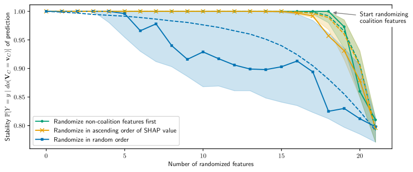
Figure 3: Stability of the prediction on the South German Credit dataset with respect to randomization of features. We randomize the values of the features in increasing order based on the SHAP values (blue), while ensuring that the features of the minimal coalition identified by ICECREAM are randomized last (green), and in completely random order (red). For the randomized features we pick 1,000 samples from their data distribution and check whether the model output changes. We do this for the sample mentioned in Example 2 (solid lines) and over all samples for which a coalition with four or less components was identified (dashed line and colored area representing average and 95% quantile). The model prediction remains stable as long as the features in the minimal coalition identified by ICECREAM remain fixed. When strictly following the SHAP value order, the prediction shows a very similar behavior.

5.2 Explaining issues in a cloud computing application

We consider a cloud computing application in which services call each other to produce a result which is returned to the user at the target service $Y$. Services can either be stand-alone (like a database or a random number generator) or call other services and transform their input to produce an output. When we observe an error at the target service $Y$, we want to know which service(s) caused this error. To imitate such a system, we synthetically generate data from a system with ten binary variables. Each variable represents a service with an intrinsic error rate $p_{i}\in[0,1]$ and a threshold $t_{i}\in\{0,...,|\bm{P\!A}_{i}|\}$ which determines how many parent services must experience an error such that the error is propagated. The specific network and parameters that we are using for sample generation can be found in Section C.3. To obtain a representative set of observations with errors at the target service, we generate 10 million samples from the joint distribution and select the ones where $Y=1$. The actual ground truth root causes of these errors are the noise variables $\Lambda_{i}$ with $\Lambda_{i}=1$, but for our experiments we consider them as unobserved and only use observations from the variables $\bm{X}$.

We compare ICECREAM to the root cause analysis (RCA) approaches presented by Budhathoki et al., (2022). We use this method with different anomaly detection methods: an information theoretic outlier score (IT-RCA), and a score based on the mean deviation (Mean-RCA). Additionally, we evaluate both methods with a cumulative threshold (picking features in ascending SHAP order until the sum of their contribution scores reaches a threshold, denoted with -c) and an individual threshold (picking all features whose individual contribution value reaches the threshold, denoted with -i). Finally, we add a simple traversal algorithm as baseline where we identify anomalies and consider the first anomaly in the graph as the root cause of the issue (see Section C.3.3).

For ICECREAM we consider the set of noise variables $\Lambda$ as the potential root causes and hence look for the minimal coalition $\bm{V}_{C}=\bm{\Lambda}_{C}$ explaining an error at the target service $Y$. This choice follows the argumentation in Budhathoki et al., (2022). The advantage of intervening on the noise variables is that the connections among the observed variables remain unchanged. This way it is possible to identify the variable which shows not just anomalous behavior per se, but anomalous behavior conditioned on the behavior of its parents. This allows us to identify the actual root cause of an event, instead of just identifying the variable with the most abnormal behavior. However, intervening on the unobserved noise variables is highly non-trivial in practice. Nevertheless, for the error propagation in this application we can estimate the conditional noise distribution $\mathbb{P}[\bm{\Lambda}\mid\bm{X}=\bm{x}]$ from the observations given the dependency structure of the application. With this we are able to compute an expected explanation score over this noise distribution: $\bar{\mathcal{E}}_{\bm{v}}(\bm{\Lambda}_{C}):=\mathbb{E}_{\bm{\lambda}\sim\bm{\Lambda}\mid\bm{X}=\bm{x}}[\mathcal{E}_{\bm{\lambda}}(\bm{\Lambda}_{C})]$.

We compare the methods with respect to accuracy, as well as true positives, false positives, and false negatives. For ICECREAM, the root cause of a sample counts as correctly identified if and only if all identified minimal coalitions are correct. For the other methods, the root cause counts as correctly identified if the returned set of root causes is correct. Figure 4 shows the performance of the methods for different numbers of errors injected into the system. It is evident that ICECREAM is the only method which still achieves close to 100% accuracy when the number of errors increases.

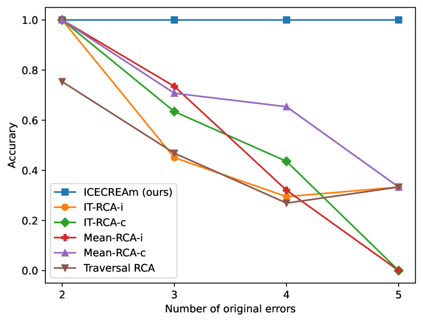
(a) Accuracy of identifying root causes for different numbers of injected errors.

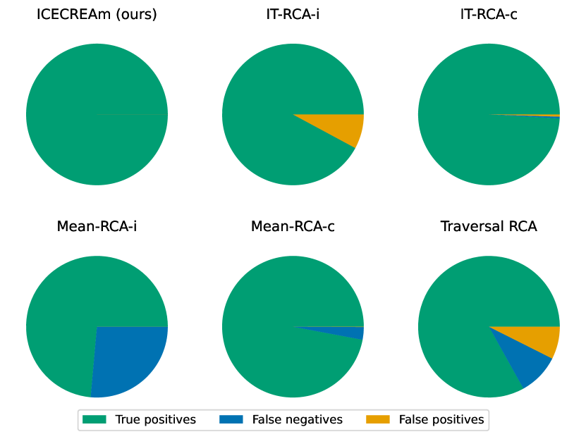
(b) True positives, false positives, and false negatives for the cases with at least 3 injected errors.

Figure 4: Accuracy for the identification of root causes of issues in a cloud computing application. If the ground truth root cause only consists of two errors in the system, most methods for RCA are able to identify them with 100% accuracy. However, if the issue is the result of a combination of more than two errors, only ICECREAM is able to identify the coalition of failing services correctly, while the performance of the other RCA methods drops drastically.

6 Conclusion

In this paper, we proposed a novel approach for explainability and causal contribution analysis which is able to identify minimal coalitions of variables that are required to explain a target value. We presented an explanation score which provides a quantitative, information-theoretic measure for the relative shift in the target distribution caused by an intervention on a coalition of variables, compared to the distribution before the intervention and the point mass distribution corresponding to the actual observation. This score satisfies all desired properties in order to explain target values which are the result of an interaction of multiple factors. Additionally, we proved some beneficial properties of the score which, for instance, allow for an easy interpretation of the score, and also allow us to use the explanation score to identify optimal interventions to change the target value.

Our experiments show that ICECREAM achieves similar performance in explaining an ML model as the established SHAP values, while providing more concise information about coalitions instead of just a ranking of feature contributions. Moreover, it clearly outperforms state-of-the-art RCA methods in identifying the root cause of an issue, particularly when this is a combination of multiple factors.

The ICECREAM framework is sufficiently generic to be applied to any causal network; however, our current formulation relies on a few assumptions or design choices which limit its scope. For instance, the explanation score in its current form cannot be applied for continuous target variables, since the point mass distribution $\delta_{y}$ is not a valid target distribution in this case. Additionally, for systems with many variables, iterating over all coalitions can become quite costly, particularly if no “small” coalition with “good” explanation score can be found and larger coalitions also need to be tested. This is the case despite the extremely fast estimation of the explanation score and simply caused by the combinatorial explosion for larger coalitions. In future work we will investigate how the fact that $\{C\in 2^{I}:\mathcal{E}(C)=1\}$ is an upper set of $2^{I}$ can be used to develop a more efficient search algorithm for minimal coalitions.

Appendix A Proofs

Property 1.

A coalition $\bm{V}_{C}$ gets an explanation score $\mathcal{E}_{\bm{v}}(\bm{V}_{C})>0$ if and only if fixing the coalition values brings the distribution of the target variable closer to the point mass distribution $Y\sim\delta_{y}$. $\mathcal{E}_{\bm{v}}(\bm{V}_{C})=1$ if and only if $\mathbb{P}[Y\mid do(\bm{V}_{C})]=\mathbb{P}[Y\mid do(\bm{V})]=\delta_{y}$. In this case we say the coalition fully explains the target value. Conversely, $\bm{V}_{C}$ gets an explanation score $\mathcal{E}_{\bm{v}}(\bm{V}_{C})<0$ if and only if fixing the coalition values moves the distribution of the target variable further away from the distribution $Y\sim\delta_{y}$, and it is $\mathcal{E}_{\bm{v}}(\bm{V}_{C})=0$ if and only if fixing the coalition values has no effect on the distance between the distribution of $Y$ and $\delta_{y}$.

Proof.

This directly follows from Equation 1 in Definition 1. We have

$$\mathcal{E}_{\bm{v}}(\bm{V}_{C})>0\quad \Leftrightarrow\quad 1-\frac{D(\mathbb{P}[Y\mid do(\bm{V}_{C})],\mathbb{P}[Y\mid do(\bm{V})])}{D(\mathbb{P}[Y],\mathbb{P}[Y\mid do(\bm{V})])}>0$$

$$\Leftrightarrow\quad\frac{D(\mathbb{P}[Y\mid do(\bm{V}_{C})],\mathbb{P}[Y\mid do(\bm{V})])}{D(\mathbb{P}[Y],\mathbb{P}[Y\mid do(\bm{V})])}<1$$

$$\Leftrightarrow\quad D(\mathbb{P}[Y\mid do(\bm{V}_{C})],\mathbb{P}[Y\mid do(\bm{V})])<D(\mathbb{P}[Y],\mathbb{P}[Y\mid do(\bm{V})])$$

$$\Leftrightarrow\quad\mathbb{P}[Y\mid do(\bm{V}_{C})]\text{ is closer to }\mathbb{P}[Y\mid do(\bm{V})]\text{ than }\mathbb{P}[Y]$$

$$\mathcal{E}_{\bm{v}}(\bm{V}_{C})<0\quad \Leftrightarrow\quad 1-\frac{D(\mathbb{P}[Y\mid do(\bm{V}_{C})],\mathbb{P}[Y\mid do(\bm{V})])}{D(\mathbb{P}[Y],\mathbb{P}[Y\mid do(\bm{V})])}<0$$

$$\Leftrightarrow\quad\frac{D(\mathbb{P}[Y\mid do(\bm{V}_{C})],\mathbb{P}[Y\mid do(\bm{V})])}{D(\mathbb{P}[Y],\mathbb{P}[Y\mid do(\bm{V})])}>1$$

$$\Leftrightarrow\quad D(\mathbb{P}[Y\mid do(\bm{V}_{C})],\mathbb{P}[Y\mid do(\bm{V})])>D(\mathbb{P}[Y],\mathbb{P}[Y\mid do(\bm{V})])$$

$$\Leftrightarrow\quad\mathbb{P}[Y\mid do(\bm{V}_{C})]\text{ is further away from }\mathbb{P}[Y\mid do(\bm{V})]\text{ than }\mathbb{P}[Y]$$

$$\mathcal{E}_{\bm{v}}(\bm{V}_{C})=1\quad \Leftrightarrow\quad 1-\frac{D(\mathbb{P}[Y\mid do(\bm{V}_{C})],\mathbb{P}[Y\mid do(\bm{V})])}{D(\mathbb{P}[Y],\mathbb{P}[Y\mid do(\bm{V})])}=1$$

$$\Leftrightarrow\quad\frac{D(\mathbb{P}[Y\mid do(\bm{V}_{C})],\mathbb{P}[Y\mid do(\bm{V})])}{D(\mathbb{P}[Y],\mathbb{P}[Y\mid do(\bm{V})])}=0$$

$$\Leftrightarrow\quad D(\mathbb{P}[Y\mid do(\bm{V}_{C})],\mathbb{P}[Y\mid do(\bm{V})])=0$$

$$\Leftrightarrow\quad\mathbb{P}[Y\mid do(\bm{V}_{C})]=\mathbb{P}[Y\mid do(\bm{V})]$$

$$\mathcal{E}_{\bm{v}}(\bm{V}_{C})=0\quad \Leftrightarrow\quad 1-\frac{D(\mathbb{P}[Y\mid do(\bm{V}_{C})],\mathbb{P}[Y\mid do(\bm{V})])}{D(\mathbb{P}[Y],\mathbb{P}[Y\mid do(\bm{V})])}=0$$

$$\Leftrightarrow\quad\frac{D(\mathbb{P}[Y\mid do(\bm{V}_{C})],\mathbb{P}[Y\mid do(\bm{V})])}{D(\mathbb{P}[Y],\mathbb{P}[Y\mid do(\bm{V})])}=1$$

$$\Leftrightarrow\quad D(\mathbb{P}[Y\mid do(\bm{V}_{C})],\mathbb{P}[Y\mid do(\bm{V})])=D(\mathbb{P}[Y],\mathbb{P}[Y\mid do(\bm{V})])$$

$$\Leftrightarrow\quad\mathbb{P}[Y\mid do(\bm{V}_{C})]\text{ is as close to }\mathbb{P}[Y\mid do(\bm{V})]\text{ as }\mathbb{P}[Y]$$

∎

Property 2.

If a variable $V_{i}\in\bm{V}$ is irrelevant for $Y$, i.e., $\mathbb{P}[Y\mid do(V_{i}=v_{i})]=\mathbb{P}[Y\mid do(V_{i}=v_{i}^{\prime})]$ for all $v_{i},v_{i}^{\prime}\in\mathcal{V}_{i}$, then $\mathcal{E}_{\bm{v}}(\bm{V}_{C})=\mathcal{E}_{\bm{v}}(\bm{V}_{C}\cup\{V_{i}\})\;\forall\bm{v}\in\bm{\mathcal{V}},\bm{V}_{C}\subseteq\bm{V}\setminus\{V_{i}\}$.

Proof.

If $V_{i}$ is irrelevant for $Y$, the distribution of $Y$ does not change when we fix $V_{i}=v_{i}$, and therefore $\mathbb{P}[Y]=\mathbb{P}[Y\mid do(V_{i})]$ as well as $\mathbb{P}[Y\mid do(\bm{V}_{C})]=\mathbb{P}[Y\mid do(\bm{V}_{C}\cup\{V_{i}\})]$. ∎

Property 3.

If $\mathcal{E}_{\bm{v}}(\bm{V}_{C})=1$ for some $\bm{V}_{C}\subseteq\bm{V}$, then $\mathcal{E}_{\bm{v}}(\bm{V}_{C^{\prime}})=1$ for all $C^{\prime}\supseteq C$.

Proof.

We assume without loss of generality that $\bm{V}_{C^{\prime}}=\bm{V}_{C}\cup\{V_{i}\}$, $V_{i}\notin\bm{V}_{C}$. Then we have

$$\mathcal{E}_{\bm{v}}(\bm{V}_{C})=1\quad {\Leftrightarrow}\quad D(\mathbb{P}[Y\mid do(\bm{V}_{C})],\mathbb{P}[Y\mid do(V)])=0$$

$$\Rightarrow\quad\mathbb{P}[Y\mid do(\bm{V}_{C})]=\mathbb{P}[Y\mid do(V)]=\delta_{y}$$

$${\Rightarrow}\quad\mathbb{P}[Y=y\mid do(\bm{V}_{C})]=1$$

$${\Rightarrow}\quad\mathbb{P}[Y=y\mid do(\bm{V}_{C}),do(V_{i}=v_{i})]=1\quad\forall v_{i}\in\mathcal{V}_{i}$$

$$\phantom{{\Rightarrow}\quad\mathbb{P}[Y=y\mid do(\bm{V}_{C}),do(V_{i}=v_{i})]=1}\text{ with }\mathbb{P}[Y=y,\bm{V}_{C}=\bm{v}_{C},V_{i}=v_{i}]>0$$

$${\Rightarrow}\quad\mathbb{P}[Y=y\mid do(\bm{V}_{C^{\prime}})]=1$$

$${\Leftrightarrow}\quad\mathbb{P}[Y\mid do(\bm{V}_{C^{\prime}})]=\mathbb{P}[Y\mid do(V)]$$

$${\Leftrightarrow}\quad D(\mathbb{P}[Y\mid do(\bm{V}_{C^{\prime}})],\mathbb{P}[Y\mid do(V)])=0\quad{\Leftrightarrow}\quad\mathcal{E}_{\bm{v}}(\bm{V}_{C^{\prime}})=1\;.$$

∎

Property 4.

If $\mathcal{E}_{\bm{v}}(\bm{V}_{C})=1$ for some $\bm{V}_{C}\subseteq\bm{V}$, then there exists no $V_{i}\in\bm{V}\setminus\bm{V}_{C}$ such that changing the value of $V_{i}$ changes the value of the target $Y$. Further, to change the target value from $y$ to $y^{*}$, at least a subset $\bm{V}_{S}\subseteq\bm{V}_{C},\bm{V}_{S}\neq\varnothing$ needs to change its values from $\bm{v}_{S}$ to some $\bm{v}^{*}_{S}$.

Proof.

For a coalition $\bm{V}_{C}$ with full explanation score, changing any non-coalition variables does not affect the target variable:

$$\mathcal{E}_{\bm{v}}(\bm{V}_{C})=1 \quad{\Leftrightarrow}\quad D(\mathbb{P}[Y\mid do(\bm{V}_{C})],\mathbb{P}[Y\mid do(V)])=0$$

$$\quad{\Rightarrow}\quad\mathbb{P}[Y=y\mid do(\bm{V}_{C})]=1$$

$$\quad{\Rightarrow}\quad\mathbb{P}[Y=y\mid do(\bm{V}_{C}),do(V_{i}=v_{i})]=1\quad\forall v_{i}\in\mathcal{V}_{i},V_{i}\notin\bm{V}_{C}$$

$$\phantom{{\Rightarrow}\quad\mathbb{P}[Y=y\mid do(\bm{V}_{C}),do(V_{i}=v_{i})]=1}\text{ with }\mathbb{P}[Y=y,\bm{V}_{C}=\bm{v}_{C},V_{i}=v_{i}]>0$$

$$\quad{\Rightarrow}\quad\mathbb{P}[Y=y^{*}\neq y\mid do(\bm{V}_{C}),do(V_{i})]=0\quad\forall v_{i}\in\mathcal{V}_{i},V_{i}\notin\bm{V}_{C}$$

From Property 3 it follows that there exists a minimal coalition $\bm{V}_{min}\subseteq\bm{V}_{C}$ with full explanation score, which cannot be empty by construction of the explanation score (remember that $\mathcal{E}(\bm{V}_{\varnothing})$ is always $0$). If we remove another element $V_{i}$ from $\bm{V}_{min}$, the explanation score will be $<1$ and thus the probability for target values $y^{*}\neq y$ becomes non-zero. ∎

Appendix B Applying Shapley-based approaches to coalitions of variables

In this section, we discuss how Shapley-based approaches can be applied to quantify the contribution of coalitions of variables.

First, we consider a simple, intuitive approach that allows us to apply well-established Shapley-based contribution methods for individual variables (e.g. Lundberg and Lee,, 2017; Frye et al.,, 2020; Heskes et al.,, 2020; Wang et al.,, 2020; Janzing et al.,, 2020, 2021; Jung et al.,, 2022) to coalitions of variables. The idea is to merge variables belonging to the respective coalition into a “super-variable” (which can be one- or multi-dimensional). For instance, in the example shown in Figure 5(a), the variables $X_{1}$ and $X_{2}$ can be merged into a joint variable $X_{12}=X_{1}\lor X_{2}$ to represent the coalition of the two variables (see Figure 5(b)). Then the Shapley-based attribution methods can simply be applied to the variable $X_{12}$ to obtain a contribution score for the coalition.

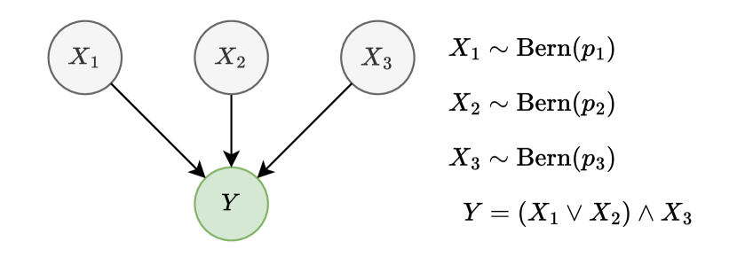
(a) Original system

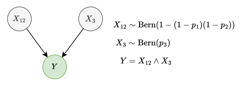
(b) System after merging coalition variables

Figure 5: Illustration how Shapley-based approaches can be applied to coalitions of variables by merging the variables accordingly. In this example we consider the coalition of $X_{1}$ and $X_{2}$. We can merge these variables into a new variable $X_{12}=X_{1}\lor X_{2}$, and then compute the Shapley-based contribution of this variable in the new graph. Note that it is not always possible to merge variables like this, depending on the functional relationships in the network. But as a general approach we can allow for multi-dimensional variables as representations of the coalitions and then merge variables by creating a vector $X_{12}=(X_{1},X_{2})$.

The efficiency property of Shapley values ensures that any Shapley-based contributions of the individual variables in the original graph, denoted here by $\phi_{X_{i}}$, sum up to some statistic of the target variable

$$\sum_{i\in I}\phi_{X_{i}}=\Phi_{Y}\,.$$ (3)

This statistic $\Phi_{Y}$ can, for instance, be the deviation from the expectation, an information-theoretic (IT) outlier score of $Y$ (see Budhathoki et al.,, 2022), or any other function which does not depend on the variables $X_{i}$, but only on the target distribution.

If we now merge the variables of a coalition $C\subset I$, we get a new graph, consisting of the “super-variable” $X_{C}$ as well as some (unchanged) variables $X_{i},i\in I\setminus C$. Calculating the Shapley-based contribution values on this new set of variables can result in new values $\psi_{X_{k}}$ for all $X_{k}\in\{X_{C}\}\cup\{X_{i}:\,i\in I\setminus C\}$. But, since this merging of variables does, by definition, not affect the target variable or its distribution, the following still holds:

$$\psi_{X_{C}}+\sum_{i\in I\setminus C}\psi_{X_{i}}=\Phi_{Y}\,.$$ (4)

Consequently, it is

$$\sum_{i\in I}\phi_{X_{i}}=\psi_{X_{C}}+\sum_{i\in I\setminus C}\psi_{X_{i}}\,.$$ (5)

Intuitively, we would expect that the contribution scores of the non-coalition variables should not depend on whether we merge the coalition variables or not, since their influence on the target has not changed. If we assume $\psi_{X_{i}}=\phi_{X_{i}}$ for all $i\in I\setminus C$, this necessarily results in the contribution of the coalition being the sum of the contributions of its components:

$$\psi_{X_{C}}=\sum_{i\in C}\phi_{X_{i}}\,.$$ (6)

To put it simply: Any Shapley-based contribution method either satisfies Equation 6 and hence violates Desideratum 1, or allows the contribution of individual variables to change depending on whether and how the other variables are grouped into coalitions. We consider both options not desirable for a contribution score to quantify the influence of coalitions.

Nevertheless, we consider examples for both options in our experiments with existing RCA methods in Section 5.2 for the comparison with ICECREAM. The first method uses the above-mentioned IT outlier score. This score leaves the contributions of the non-coalition nodes unchanged. As a result, merging variables just gives the same results as summing up the respective individual contribution values. The second approach uses a mean deviation outlier score. This score changes the contributions of the non-coalition variables, and can therefore give a non-trivial coalition contribution. Our experiments show that ICECREAM clearly outperforms both approaches in the identification of root causes in a cloud computing application for cases where multiple errors together result in a failure at the target service.

Only quite recently, more sophisticated approaches have been proposed to link Shapley values to coalitions of features, from the pairwise Shapley Interaction Values (Lundberg et al.,, 2020) to the Shapley-Taylor Interaction Index (Dhamdhere et al.,, 2020) and $n$-Shapley (Bordt and von Luxburg,, 2023). These approaches make the connections between features more transparent and therefore interpretable, but they still follow the premise that contributions have to add up. If one coalition of features is very important, the remaining features have to be less important. What is measured is basically the importance of feature sets relative to each other. Therefore, our above arguments with respect to Desideratum 1 still apply. In contrast, ICECREAM allows for independent explanation scores for all coalitions, which can be thought of describing the (causal) importance of a feature set relative to the natural target distribution and the actual observation.

Appendix C Experiments

This section provides additional details on the experiments whose basic setup and results are reported in Section 5 in the main paper.

C.1 CorrAL feature selection dataset

CorrAL is a synthetic dataset consisting of six Boolean features (A0, A1, B0, B1, Irrelevant and Correlated) and 160 samples. The feature names are rather self-explanatory as the target variable is defined as

$$\texttt{class}:=(\texttt{A0}\wedge\texttt{A1})\vee(\texttt{B0}\wedge\texttt{B1})\;.$$

The remaining two features are not used—Irrelevant is uniformly random, and Correlated matches the target label in 75% of all samples. John et al., (1994), who created the dataset as an illustration for the shortcomings of existing feature selection algorithms, report that greedy selection mechanisms (both top-down and bottom-up) have difficulties identifying the correct feature set. We therefore test ICECREAM on the full dataset and see which features are selected as part of the minimum-size coalitions with full explanation score.

As causal model for the dataset, we consider the input features to be independent, while we allow all of them to potentially influence the target. As threshold for coalitions with full explanation score we use $\alpha=0.998$ and evaluate all coalitions sizes $k\in\{1,\dots,\text{\#features}\}$.

ICECREAM easily identifies the minimal full explanations in all cases without including the irrelevant or only correlated feature into the coalitions. As an example, let us consider the first row of the dataset, where all features are False. A full explanation must consist of at least one of A0 and A1 (to explain why the first conjunction is False), plus at least one of B0 and B1. Accordingly, the minimum-size coalitions found by ICECREAM are the four combinations $\{\texttt{A0},\texttt{B0}\}$, $\{\texttt{A0},\texttt{B1}\}$, $\{\texttt{A1},\texttt{B0}\}$, and $\{\texttt{A1},\texttt{B1}\}$.

C.2 Explaining an ML model on the South German Credit dataset

The South German Credit (SGC) dataset (Grömping,, 2019) contains 1,000 loan applications with 21 features, and the corresponding risk assessment (low-risk or high-risk) as the binary target variable.

C.2.1 Model

In this experiment, we are explaining the predictions of a trained ML model on a given dataset. As the model, we use a simple random forest classifier with the pipeline shown in Figure 6, trained on the full dataset with a train/test split of 90/10. The fitted model reaches an accuracy of 96% for the training set and 80% for the test set. Note that we consider explanations for this model – not for the data itself. Hence we ignore that the model is not performing extremely well.

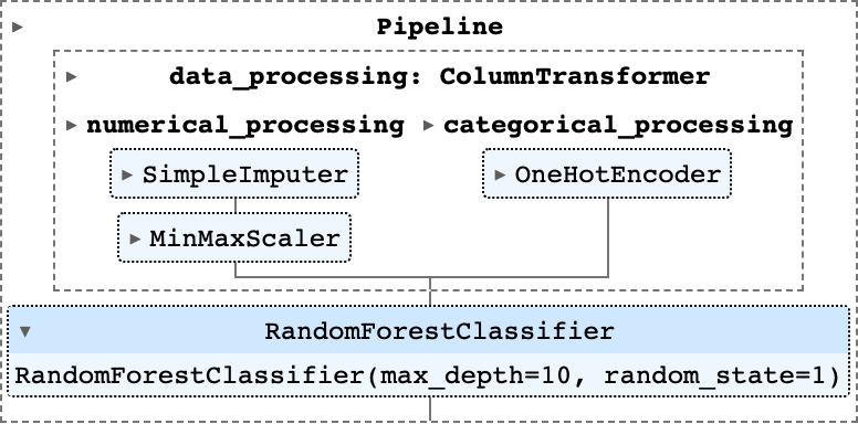
Figure 6: Training pipeline for the model used in the experiment on the SGC dataset.

C.2.2 SHAP values

To obtain the SHAP values for comparison, we make use of the shap package by Lundberg and Lee, (2017). The use of their explainer is straight-forward; note that the categorical features need to be converted into integer categories first for shap to handle the input. In Figure 7 we show the SHAP output for the sample with ID 500, the sample also shown in Table 2 and mentioned in Example 2 in the main paper.

Table 2: Feature values and SHAP values for sample 500 of the SGC dataset.

Feature	Value	SHAP value
credit_purpose	others	0.034
housing	own	0.020
personal_status	married/widowed	0.020
other_installment_plans	bank	0.019
age_groups	0	0.017
sex	male	0.017
credit_amount	7308	0.015
checking_account_status	… < 0 DM	0.015
employed_since_years	unemployed	0.014
job_status	mgmt/self-employed/highly qualified empl./officer	0.014
property	real estate	0.013
credit_history	no credits taken/all credits paid back duly	0.009
telephone	True	0.007
num_existing_credits	1	0.006
savings	unknown/no savings account	0.004
credit_duration_months	10	0.003
installment_rate	25 <= … < 35	0.002
present_residence_since	>= 7 yrs	0.001
other_debtors_guarantors	none	0.001
foreign_worker	False	0.000
num_people_liable_for	0 to 2	-0.002

Originally, SHAP values are designed to explain the difference between the actual prediction and its expected value. Since the ratio of low-risk ($\texttt{credit\_risk}=0$) and high-risk ($\texttt{credit\_risk}=1$) loan applications in the dataset is $\approx 30/70$, this difference is not always the same. We therefore normalize the SHAP values such that the feature contributions add up to 1 for each sample. This does not change the relative importance of the features, but allows for a better comparison across low-risk and high-risk samples.

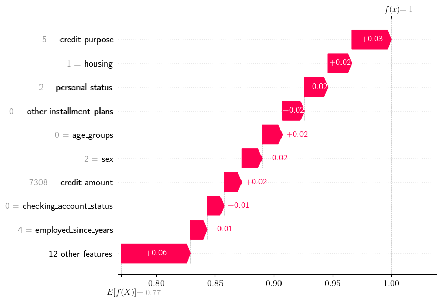
Figure 7: SHAP values for sample 500 of the SGC dataset.

C.2.3 Comparison

We compare the stability of the prediction under three different randomizations, showing the probability that the prediction remains unchanged for any number of randomized features. The underlying reasoning is: The better an explanation, the more stable the model prediction when the explanation holds (i.e., when the respective feature values are fixed). Therefore, we start with all features fixed to their observed values and successively randomize more and more features according to their joint distribution in the dataset, observing when the prediction stability drops. The three randomizations only differ in the order of features:

Randomize in ascending order of SHAP values

The features are ordered ascendingly by their SHAP value. This is the order in which the prediction can be expected to stay stable as long as possible: Randomizing features with a SHAP value $<0$ means that the negative influence of these features is removed. The features with the highest (positive) SHAP value, on the other hand, are kept fixed until much longer, such that their stabilizing influence can be used.

Randomize non-coalition features first

The features of the minimum-size full explanation identified by ICECREAM are randomized last. By doing so, we see whether the prediction is determined by the fixed values of this feature coalition. The order of the remaining features is chosen as above to maximize comparability.

Randomize in random order

As a baseline, we randomize the features in random order to see how fast the prediction stability drops when there are no “special” features.

In order to obtain the interventional distributions required in ICECREAM, we follow the reasoning of Janzing et al., (2020) and consider the real world to be a confounder of the input features of the ML model, which therefore do not have direct causal links among each other. As a consequence, we can intervene directly on the input features by simply fixing the values of the features belonging to the considered coalition while sampling the remaining features from their (joint) marginal distribution. Further, we choose a threshold of $\alpha=0.9998$ to identify coalitions with (almost) full explanations while allowing for numerical errors. Additionally, we set the maximum coalition size to $k=4$ and stop the procedure if we do not find a coalition exceeding the threshold at this size.

C.2.4 Result

Out of the $1,000$ samples in the credit dataset, $426$ have simple explanations as defined above (most of them have multiple such explanations, such that the mean and quantiles in Figure 3 are composed of 1,803 data points). On average, the cumulative normalized SHAP value of the minimum-size full explanations is $53.2\%$.

Analyzing Figure 3, we see that, on average, ICECREAM and SHAP show a similar performance, although ICECREAM’ performance for the solid-line sample (sample 500) only drops for the last 3 features while SHAP decreases a few fetures earlier. This is due to the fact that, for this sample, a 3-feature coalition is actually sufficient to reach an explanation score of $\approx 1$. Grouping the samples by the size $k$ of their minimum-size full explanation coalitions, we would see that the stability of ICECREAM is very much determined by this value, i.e., the prediction stability always drops after $|\bm{X}|-k$ features. Such a pattern cannot be observed for SHAP.

Using a random order for the randomization of features, the drop in the prediction stability starts much earlier, usually after $\approx 10$ features. Note that there is a small number of outliers even after one or two features, causing the mean to decrease immediately, while the 5-95% range is still at 1.

C.2.5 Computation

The experiment was executed on a 10-core MacBook Pro M2. The calculation of the SHAP values took $\approx 5$ minutes, while the identification of all minimum-size coalitions up to size $k=4$ took $\approx 6$ hours.

C.3 Identifying root causes in a cloud computing application

We consider a cloud computing application in which services call each other to produce a result which is returned to the user at the target service $Y$. Services can either be stand-alone (like a database or a random number generator) or call other services and transform their input to produce an output. When we observe an error at the target service $Y$, we want to know which service(s) caused this error.

C.3.1 Data generation

The causal network of the Cloud Computing Application experiment is based on a realistic service architecture shown in Figure 8. On top of the causal dependencies, we have defined parameters $p_{i}$ and $t_{i}$ such that target errors are a rare, but not impossible phenomenon. This architecture translates to the causal network shown in Figure 9 with services $X_{1},...,X_{9},Y$, by omitting the Website service and using www as the target variable. We generate synthetic data representing error counts for the different services according to

$$X_{i}=\Lambda_{i}\vee\left(\sum_{j\in\bm{P\!A}_{i}}{X_{j}}\geq t_{i}\right)\text{, where }\Lambda_{i}\sim\text{Bern}(p_{i})\;.$$ (7)

We generated $10$ million samples, of which $15,373$ samples produce a target error (i.e., $Y=1$). Table 3 shows the number of elements in the sample set, grouped by the number of original errors. We see that fewer than two original errors never lead to a target error.

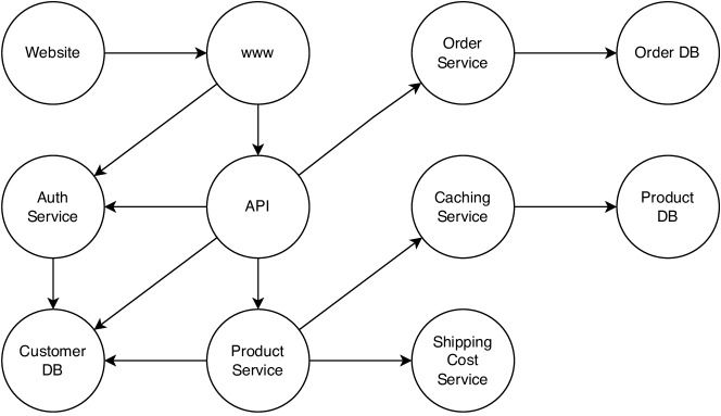
Figure 8: Cloud service architecture with non-trivial causal dependencies.

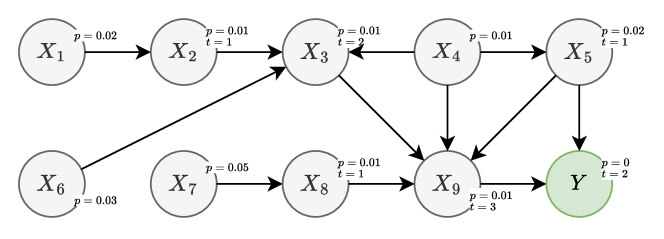
Figure 9: Causal graph of the cloud computing application in Figure 8. The parameters $p_{i}$ denote the probability that a node produces an error itself, and $t_{i}$ is the threshold number of parent services that have to encounter an error to also cause the error to propagate to $X_{i}$.

Table 3: Number of generated samples, grouped by the number of original errors, i.e., noise nodes with value 1.

# errors	# samples with $Y=0$	# samples with $Y=1$
0	8,416,434	0
1	1,471,666	0
2	93,532	14,009
3	2,953	1,283
4	42	78
5	0	3

C.3.2 Mapping from root causes to minimal coalitions

From the contribution scores produced by the RCA methods (see Budhathoki et al.,, 2022), we find minimal coalitions with the following procedure:

1. Calculate the contribution score $\Phi(i)$ for all features $i\in I$.

2. Sort the features by descending score and normalize them so that $\sum{\Phi_{i}}=1$.

3. Select feature via a cumulative threshold (take features in the above order until the sum of their contribution scores reaches a threshold $\theta_{c}=0.95$), or via an individual threshold (take all features with $\Phi(i)\geq\theta_{i}=0.15$).

The thresholds $\theta_{c}$ and $\theta_{i}$ were found through hyperparameter tuning such that these RCA methods achieve the best performance when compared to the ground truth. By applying this procedure, we get a coalition of features from all baseline methods.

C.3.3 Traversal RCA

The traversal method for RCA is based on a very simple idea: A node in the causal graph is identified as a root cause if (a) it shows an error (we say the node is anomalous), and (b) none of its causal parents is anomalous. This can be directly inferred from an observation, outputting a set of root causes.

A slightly more sophisticated way is to additionally require for a root cause to have a path of anomalous nodes to the target, therefore backtracking from the target to possible root causes (called Backtracking Traversal RCA in Figure 10). This can be implemented as a breadth-first search from the target node which stops at non-error nodes and then returns the leaves of the search tree. The effect is that a node is only identified as a root cause if there is a direct error propagation path from this node to the target, thus reducing false positives.

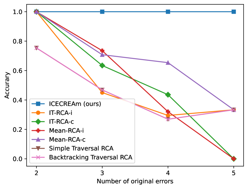
(a) Accuracy of identifying root causes for different numbers of injected errors.

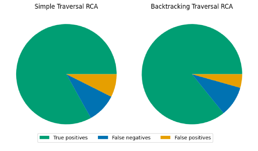
(b) True positives, false positives, and false negatives for the cases with at least 3 injected errors.

Figure 10: Comparison of Simple Traversal RCA and Backtracking Traversal RCA for the Cloud experiment. The accuracy is unaffected, while the false positive rate decreases when using backtracking.

For completeness, we show in Figure 10 a comparison between these two traversal RCA methods. Although the false positive rate, as expected, is lower for Backtracking Traversal RCA, the accuracy remains the same: The main failure mode of Traversal RCA is the implicit assumption that a single anomalous parent is enough to prevent a node from being a root cause. This weakness is present in both versions of the algorithm, as witnessed by the high rate of false negatives.

C.3.4 Computation

Most of the experiment and analysis was executed on a 10-core MacBook Pro M2. Identifying all minimum-size coalitions for the 15,000 target error samples took approximately one hour; the traversal algorithms did not take any substantial amount of time ($<20$ seconds). However, calculating the anomaly scores for the RCA approaches using dowhy.gcm (Blöbaum et al.,, 2022) turned out to be much slower, such that this task was transferred to 10 EC2 instances and finished after about two days.

References

- Blöbaum et al., (2022) Blöbaum, P., Götz, P., Budhathoki, K., Mastakouri, A. A., and Janzing, D. (2022). Dowhy-gcm: An extension of dowhy for causal inference in graphical causal models. arXiv preprint arXiv:2206.06821.
- Bordt and von Luxburg, (2023) Bordt, S. and von Luxburg, U. (2023). From Shapley values to generalized additive models and back. In International Conference on Artificial Intelligence and Statistics, pages 709–745. PMLR.
- Budhathoki et al., (2022) Budhathoki, K., Minorics, L., Blöbaum, P., and Janzing, D. (2022). Causal structure-based root cause analysis of outliers. In International Conference on Machine Learning, pages 2357–2369. PMLR.
- Burkart and Huber, (2020) Burkart, N. and Huber, M. F. (2020). A survey on the explainability of supervised machine learning. J. Artif. Intell. Res., 70:245–317.
- Chen et al., (2018) Chen, J., Song, L., Wainwright, M. J., and Jordan, M. I. (2018). Learning to explain: An information-theoretic perspective on model interpretation. In International Conference on Machine Learning.
- Dhamdhere et al., (2020) Dhamdhere, K., Agarwal, A., and Sundararajan, M. (2020). The shapley taylor interaction index. In Proceedings of the 37th International Conference on Machine Learning, ICML’20. JMLR.org.
- Emmert-Streib et al., (2020) Emmert-Streib, F., Yli-Harja, O., and Dehmer, M. (2020). Explainable artificial intelligence and machine learning: A reality rooted perspective. Wiley Interdisciplinary Reviews: Data Mining and Knowledge Discovery, 10.
- Frye et al., (2020) Frye, C., Rowat, C., and Feige, I. (2020). Asymmetric shapley values: Incorporating causal knowledge into model-agnostic explainability. In Proceedings of the 34th International Conference on Neural Information Processing Systems, NeurIPS’20, Red Hook, NY, USA. Curran Associates Inc.
- Fryer et al., (2021) Fryer, D. V., Strümke, I., and Nguyen, H. (2021). Shapley values for feature selection: The good, the bad, and the axioms. IEEE Access, PP:1–1.
- Gerlings et al., (2021) Gerlings, J., Shollo, A., and Constantiou, I. (2021). Reviewing the need for explainable artificial intelligence (xai).
- Grabisch and Roubens, (1999) Grabisch, M. and Roubens, M. (1999). “An axiomatic approach to the concept of interaction among players in cooperative games”. International Journal of Game Theory, 28:547–565.
- Grömping, (2019) Grömping, U. (2019). South German Credit Data: Correcting a Widely Used Data Set.
- Halpern and Hitchcock, (2015) Halpern, J. Y. and Hitchcock, C. (2015). Graded causation and defaults. British Journal for the Philosophy of Science, 66(2):413–457.
- Heskes et al., (2020) Heskes, T., Sijben, E., Bucur, I. G., and Claassen, T. (2020). Causal Shapley Values: Exploiting Causal Knowledge to Explain Individual Predictions of Complex Models. arXiv 2011.01625.
- Janzing et al., (2021) Janzing, D., Blöbaum, P., Minorics, L., Faller, P., and Mastakouri, A. (2021). Quantifying intrinsic causal contributions via structure preserving interventions. arXiv 2007.00714.
- Janzing et al., (2020) Janzing, D., Minorics, L., and Bloebaum, P. (2020). Feature relevance quantification in explainable AI: A causal problem. In AISTATS 2020.
- Jethani et al., (2023) Jethani, N., Saporta, A., and Ranganath, R. (2023). Don’t be fooled: label leakage in explanation methods and the importance of their quantitative evaluation. arXiv 2302.12893.
- John et al., (1994) John, G. H., Kohavi, R., and Pfleger, K. (1994). Irrelevant Features and the Subset Selection Problem. In Cohen, W. W. and Hirsh, H., editors, Machine Learning Proceedings 1994, pages 121–129. Morgan Kaufmann, San Francisco (CA).
- Jung et al., (2022) Jung, Y., Kasiviswanathan, S., Tian, J., Janzing, D., Bloebaum, P., and Bareinboim, E. (2022). On measuring causal contributions via do-interventions. In Chaudhuri, K., Jegelka, S., Song, L., Szepesvari, C., Niu, G., and Sabato, S., editors, Proceedings of the 39th International Conference on Machine Learning, volume 162 of Proceedings of Machine Learning Research, pages 10476–10501. PMLR.
- Keane and Smyth, (2020) Keane, M. T. and Smyth, B. (2020). Good counterfactuals and where to find them: A case-based technique for generating counterfactuals for explainable ai (xai). In Watson, I. and Weber, R., editors, Case-Based Reasoning Research and Development, pages 163–178, Cham. Springer International Publishing.
- Koller and Sahami, (1996) Koller, D. and Sahami, M. (1996). Toward optimal feature selection. Technical Report 1996-77, Stanford InfoLab / Stanford InfoLab.
- Kumar et al., (2020) Kumar, I. E., Venkatasubramanian, S., Scheidegger, C., and Friedler, S. A. (2020). Problems with shapley-value-based explanations as feature importance measures. In Proceedings of the 37th International Conference on Machine Learning, ICML’20. JMLR.org.
- Lundberg et al., (2020) Lundberg, S. M., Erion, G., Chen, H., DeGrave, A., Prutkin, J. M., Nair, B., Katz, R., Himmelfarb, J., Bansal, N., and Lee, S.-I. (2020). From local explanations to global understanding with explainable ai for trees. Nature machine intelligence, 2(1):56–67.
- Lundberg and Lee, (2017) Lundberg, S. M. and Lee, S.-I. (2017). A unified approach to interpreting model predictions. In Proceedings of the 31st International Conference on Neural Information Processing Systems, NeurIPS’17, pages 4768–4777, Red Hook, NY, USA. Curran Associates Inc.
- Masoomi et al., (2020) Masoomi, A., Wu, C., Zhao, T., Wang, Z., Castaldi, P., and Dy, J. (2020). Instance-wise feature grouping. In Laroachelle, H., Ranzato, M., Hadsell, R., Balcan, M., and Lin, H., editors, Advances in Neural Information Processing Systems, volume 33, pages 13374–13386. Curran Associates, Inc.
- Mastakouri et al., (2019) Mastakouri, A., Schölkopf, B., and Janzing, D. (2019). Selecting causal brain features with a single conditional independence test per feature. Advances in Neural Information Processing Systems, 32.
- Mastakouri et al., (2021) Mastakouri, A. A., Schölkopf, B., and Janzing, D. (2021). Necessary and sufficient conditions for causal feature selection in time series with latent common causes. In International Conference on Machine Learning, pages 7502–7511. PMLR.
- Pearl, (1999) Pearl, J. (1999). Probabilities Of Causation: Three Counterfactual Interpretations And Their Identification. Synthese. An International Journal for Epistemology, Methodology and Philosophy of Science, 121(1):93–149.
- Pearl, (2009) Pearl, J. (2009). Causality: Models, Reasoning and Inference. Cambridge University Press, second edition.
- Peters et al., (2017) Peters, J., Janzing, D., and Schlkopf, B. (2017). Elements of Causal Inference: Foundations and Learning Algorithms. The MIT Press.
- Ribeiro et al., (2016) Ribeiro, M., Singh, S., and Guestrin, C. (2016). “Why Should I Trust You?”: Explaining the predictions of any classifier. pages 97–101.
- Rubin, (2005) Rubin, D. B. (2005). Causal inference using potential outcomes. Journal of the American Statistical Association, 100(469):322–331.
- Sani et al., (2021) Sani, N., Malinsky, D., and Shpitser, I. (2021). Explaining the behavior of black-box prediction algorithms with causal learning. arXiv 2006.02482.
- Shapley, (1951) Shapley, L. S. (1951). Notes on the N-Person Game — II: The Value of an N-Person Game. RAND Corporation, Santa Monica, CA.
- Shrikumar et al., (2017) Shrikumar, A., Greenside, P., and Kundaje, A. (2017). Learning important features through propagating activation differences. In Proceedings of the 34th International Conference on Machine Learning - Volume 70, ICML’17, page 3145–3153. JMLR.org.
- Singh et al., (2023) Singh, R., Miller, T., Lyons, H., Sonenberg, L., Velloso, E., Vetere, F., Howe, P., and Dourish, P. (2023). Directive explanations for actionable explainability in machine learning applications. ACM Trans. Interact. Intell. Syst.
- Spirtes et al., (1993) Spirtes, P., Glymour, C., and Scheines, R. (1993). Causation, Prediction, and Search. Springer-Verlag, New York, NY.
- Sundararajan et al., (2017) Sundararajan, M., Taly, A., and Yan, Q. (2017). Axiomatic attribution for deep networks. In Precup, D. and Teh, Y. W., editors, Proceedings of the 34th International Conference on Machine Learning, volume 70 of Proceedings of Machine Learning Research, pages 3319–3328. PMLR.
- Tritscher et al., (2023) Tritscher, J., Krause, A., and Hotho, A. (2023). Feature relevance xai in anomaly detection: Reviewing approaches and challenges. Frontiers in Artificial Intelligence, 6.
- von Kügelgen et al., (2023) von Kügelgen, J., Mohamed, A., and Beckers, S. (2023). Backtracking counterfactuals. Conference on Causal Learning and Reasoning (CLeaR).
- Wang et al., (2020) Wang, J., Wiens, J., and Lundberg, S. M. (2020). Shapley flow: A graph-based approach to interpreting model predictions. In International Conference on Artificial Intelligence and Statistics.
- Wildberger et al., (2023) Wildberger, J., Guo, S., Bhattacharyya, A., and Schölkopf, B. (2023). On the interventional kullback-leibler divergence. arXiv 2302.05380.
- Yoon et al., (2019) Yoon, J., Jordon, J., and van der Schaar, M. (2019). INVASE: Instance-wise variable selection using neural networks. In International Conference on Learning Representations.
- Zhang et al., (2022) Zhang, Y., Weng, Y., and Lund, J. (2022). Applications of explainable artificial intelligence in diagnosis and surgery. Diagnostics, 12(2).