Addressing the checkerboard problem in an Eulerian meshless method for incompressible flows

Abstract

In this paper, we look at the pressure checkerboard problem that arises in an Eulerian meshless method that solves the incompressible Navier-Stokes equations using the generalized finite difference method (GFDM). Although, the checkerboard problem has been dealt with extensively in mesh-based methods, the literature in connection with meshless methods is comparatively scarce. In this paper, we explore the occurrence of the checkerboard problem in a meshless method. A few unsuccessful attempts to resolve the checkerboard problem are reported. The successful fix for the problem entails an algorithm that adapts the point cloud by adding points in the regions of pressure oscillations. The algorithm uses an error indicator that detects the presence of the checkerboard oscillations in the solution. The algorithm minimizes the computational effort since it ensures the use of additional points only in regions of concern, as directed by the error indicator, in contrast to an approach of using a highly refined set of points throughout the domain. It also requires no a priori estimates of the regions where the oscillations occur and integrates conveniently in the framework of the meshless method since no re-meshing strategies are involved. The results are compared with literature and a good match is observed.

[inst1]organization=Indian Institute of Technology Delhi,addressline= Hauz Khas, postcode=110016, state=New Delhi, country=India

1 Introduction

The issue of checkerboard patterns in numerical solutions to incompressible flows is a fairly well-explored problem in which oscillating pressure fields of high frequency that are physically incorrect, develop as a part of the numerical solution. The numerical discretization fails to detect these oscillations, thus, permitting a non-physical solution to evolve and sometimes, converge. One of the first and perhaps the most popular solutions to this problem was proposed by Patankar and Spalding[1], in which they used different grids for storing pressure and velocity that were staggered with respect to each other. The staggering allows the discretization to accurately evaluate pressure gradients at the velocity grid nodes, without missing the checkerboard oscillations. While the method of staggered grids works well, it is unsuitable for curvilinear meshes and flows involving complex geometries. Also, the amount of book-keeping increases while using staggered grids. A popular alternate to solve the checkerboard problem was proposed by Rhie and Chow [2]. In this approach, the grid remains collocated i.e. pressure and velocity are stored at the same points unlike the staggered grid. However, in the evaluation of the face velocities, as a part of the flux calculation of the finite-volume method, a correction is introduced in terms of the third derivative of pressure. This term acts as a damping mechanism to suppress the formation of high frequency checkerboard oscillations [3]. The Rhie-Chow method and its variants have been used successfully under the umbrella of momentum interpolation methods for collocated grids[4, 5, 6, 7, 8]. A.W.Date [9, 10, 11] proposed an alternate method using collocated grids where the pressure gradient interpolation helps suppress the numerical oscillations. In addition to the two popular fixes, there have also been attempts to fix the checkerboard problem by using different differencing schemes for pressure and velocity such as one-sided differencing [12] and using pressure gradients in the estimates of velocity gradients [13].

Meshless methods have been employed for solving incompressible flows in both Eulerian framework and Lagrangian framework. Among the Eulerian approaches, radial basis function methods[14, 15, 16, 17] and moving least squares methods [18, 19] are quite popular. In the Lagrangian framework, SPH has been one of the most popular approaches[20, 21, 22, 23, 24, 25] to solve incompressible flows using both an incompressible and a weakly compressible formulation. Besides SPH, the generalized finite difference method has been applied to a wide range of problems with incompressible flows [26, 27, 28, 29]. Although the literature on checkerboard patterns is quite abundant in mesh-based methods as described above, the same in the context of meshless methods is quite scarce. There are mentions of pressure oscillations in SPH literature. For SPH, the approach of Monaghan [24] in using an artificial viscosity term to suppress non-physical oscillations is quite popular. Fatehi et al. [30, 31] modified the mass conservation equation to include pressure gradients and this is reported to reduce spurious oscillations in pressure. Pita et al. [32] used diffusive terms in the mass conservation equation as a mechanism to suppress oscillations. In the context of the generalized finite difference method (GFDM) for both Eulerian and Lagrangian simulations, a damping factor used in the pressure update possibly helps suppress non-physical oscillations [19]. In Lagrangian methods, it is not clear and remains to be ascertained if the movement of points every time-step adds numerical dissipation to the system, thus, helping with suppression of oscillations.

The focus of this work is to study the development of checkerboard oscillations in an Eulerian meshless method based on GFDM and propose a method to suppress them. The problem, in general, is countered either by using very fine sets of points that prove to be computationally expensive or by adding artificial terms to the governing equations to suppress oscillations. Although these methods have solved the problem to a certain degree, in this paper, we look at a method that adaptively refines the set of points in regions where checkerboard oscillations emerge and as a result, suppresses the oscillations with a small number of added points and with no artificial terms added to the governing equations. This paper also documents a few unsuccessful attempts to resolve the checkerboard problem in the context of Eulerian meshless methods. The purpose of documenting these attempts is to either rule them out as solutions to the checkerboard problem or to facilitate further research along these directions.

The layout of the paper is as follows. Sec. 2 describes the governing equations, the projection method and the generalized finite difference method (GFDM). Sec. 3 describes the checkerboard problem in detail, as observed in the Eulerian GFDM approach. This section lists some of the unsuccessful attempts at resolving the problem, carried out as a part of this work. We, then, go on to analyze why the pressure checkerboard problem persists in the meshfree framework by drawing parallels from mesh-based methods. Sec. 4 proposes a solution based on point cloud adaptation. Sec. 5 presents test cases for the lid-driven cavity problem at high Reynolds numbers ($R_{e}$) and evaluates the proposed solution. Sec. 6 presents the conclusions.

2 Methods

2.1 Governing Equations

The incompressible Navier-Stokes equations are considered.

$$\frac{\partial u}{\partial x}+\frac{\partial v}{\partial y}=0$$ (1)

$$\frac{\partial u}{\partial t}+\frac{\partial(u^{2})}{\partial x}+\frac{\partial(uv)}{\partial y}=-\frac{1}{\rho}\frac{\partial p}{\partial x}+\nu\Big{(}\frac{\partial^{2}u}{\partial x^{2}}+\frac{\partial^{2}u}{\partial y^{2}}\Big{)}$$ (2)

$$\frac{\partial v}{\partial t}+\frac{\partial(uv)}{\partial x}+\frac{\partial(v^{2})}{\partial y}=-\frac{1}{\rho}\frac{\partial p}{\partial y}+\nu\Big{(}\frac{\partial^{2}v}{\partial x^{2}}+\frac{\partial^{2}v}{\partial y^{2}}\Big{)}$$ (3)

where $u$,$v$ denote $x$ and $y$ components of velocity and $p$ denotes pressure. $\rho$ and $\nu$ denote density and kinematic viscosity.
The projection method [33] is used to solve the above equations. The momentum equations are first marched to solve for a provisional velocity field.

$$\frac{u_{i}^{*}-u_{i}^{n}}{\Delta t}+C_{u}|^{n}=-\frac{1}{\rho}\frac{\partial p}{\partial x}\Big{|}^{n}+V_{u}|^{n}$$ (4)

$$\frac{v_{i}^{*}-v_{i}^{n}}{\Delta t}+C_{v}|^{n}=-\frac{1}{\rho}\frac{\partial p}{\partial y}\Big{|}^{n}+V_{v}|^{n}$$ (5)

The convective and viscous terms are denoted as $C_{u}$, $C_{v}$ and $V_{u}$, $V_{v}$ respectively. The superscript ’n’ denotes the time level and ’*’ denotes the provisional values. The provisional velocity field does not satisfy the divergence-free condition. A correction pressure $p_{c}$ is computed from the Poisson equation.

$$\nabla^{2}p_{c}=\frac{\rho}{\Delta t}\nabla\cdot\vec{V}^{*}$$ (6)

Here, $\vec{V}^{*}=[u^{*},v^{*}]$. The velocity and pressure are corrected using the correction pressure as

$$u^{n+1} = u^{*}-\frac{\Delta t}{\rho}\frac{\partial p_{c}}{\partial x}$$ (7)

$$v^{n+1} = v^{*}-\frac{\Delta t}{\rho}\frac{\partial p_{c}}{\partial y}$$ (8)

$$p^{n+1} = p^{n}+p_{c}$$ (9)

2.2 The Generalized Finite Difference Method (GFDM)

The generalized finite difference method is a meshless method that estimates derivatives of flow variables from a set of neighbours that are a part of a point cloud using a weighted least squares error minimization procedure as discussed below [34, 35].
Consider a point $i$ which has a neighbourhood of points $j\in S_{i}$. $S_{i}$ denotes the support region around the point $i$. This is illustrated in Fig. 1.

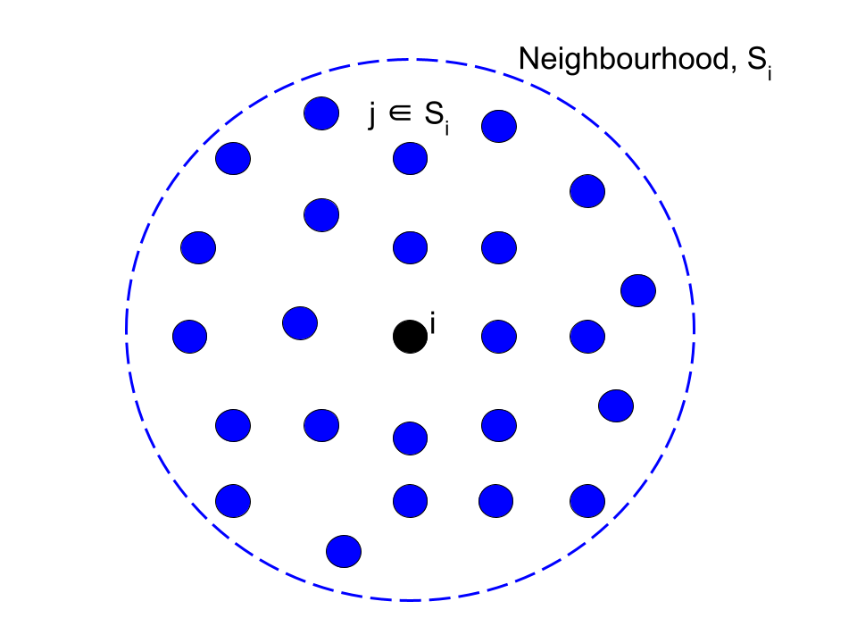
Figure 1: Generalized Finite Difference Method: Neighbourhood of a point in the point cloud.

For a given operator, there are consistency conditions that are required to be satisfied when applied on monomials up to a prescribed degree, which is usually 2. These monomials are

$$M=\begin{bmatrix}1&\Delta x&\Delta y&\Delta x^{2}&\Delta y^{2}&\Delta x\Delta y\\ \end{bmatrix}$$ (10)

Here, $\Delta x=x-x_{i}$ and $\Delta y=y-y_{i}$. Now, we derive the procedure for the Laplacian operator. The process is identical for any other operator. Let us denote the Laplacian operator at a point $j$ in the neighbourhood of point $i$ as $C^{\Delta}_{ij}$. Applying Laplacian the operator to each of the monomials in Eq. 10, we get

$$\sum_{j\in S_{i}}C^{\Delta}_{ij}(1) = 0$$ (11)

$$\sum_{j\in S_{i}}C^{\Delta}_{ij}(\Delta x_{j}) = 0$$ (12)

$$\sum_{j\in S_{i}}C^{\Delta}_{ij}(\Delta y_{j}) = 0$$ (13)

$$\sum_{j\in S_{i}}C^{\Delta}_{ij}(\Delta x_{j}^{2}) = 2$$ (14)

$$\sum_{j\in S_{i}}C^{\Delta}_{ij}(\Delta y_{j}^{2}) = 2$$ (15)

$$\sum_{j\in S_{i}}C^{\Delta}_{ij}(\Delta x_{j}\Delta y_{j}) = 0$$ (16)

This can be rewritten in matrix form as

$$\textbf{V}\vec{C^{\Delta}}=\vec{b}$$ (18)

where, $\text{V}=\begin{pmatrix}.&.&.&1&.&.&.\\ .&.&.&\Delta x_{j}&.&.&.\\ .&.&.&\Delta y_{j}&.&.&.\\ .&.&.&\Delta x_{j}^{2}&.&.&.\\ .&.&.&\Delta y_{j}^{2}&.&.&.\\ .&.&.&\Delta x_{j}\Delta y_{j}&.&.&.\\ \end{pmatrix}$ $\vec{C^{\Delta}}=\begin{pmatrix}C^{\Delta}_{i1}\\ .\\ .\\ C^{\Delta}_{ij}\\ .\\ .\\ C^{\Delta}_{iN}\\ \end{pmatrix}$ $\vec{b}=\begin{pmatrix}0\\ 0\\ 0\\ 2\\ 2\\ 0\\ \end{pmatrix}$. Eq. 18 is used in minimizing the functional

$$J=\sum\frac{(C^{\Delta}_{ij})^{2}}{w_{ij}}$$ (19)

This gives

$$\vec{C^{\Delta}}=\textbf{W}\textbf{V}^{T}(\textbf{V}\textbf{W}\textbf{V}^{T})^{-1}\vec{b}$$ (20)

where W is a diagonal matrix with its entries given by the weight of the point $j\in S_{i}$ w.r.t. point $i$, $\textbf{W}=\begin{pmatrix}w_{i1}&0&0&.&.\\ 0&w_{i2}&0&.&.\\ .&.&.&.&.\\ &&.&.&w_{iN}\\ \end{pmatrix}$
Having derived the Laplacian operator from Eq. 20, the Laplacian of a general function $\phi$ at the point $i$ may be written as

$$\nabla^{2}\phi|_{i}=\sum_{j\in S_{i}}C^{\Delta}_{ij}\phi_{j}$$ (21)

For the first derivatives in $x$ and $y$, the operator $C^{\Delta}_{ij}$ in Eq. 21 is simply replaced with the corresponding operator - $C^{x}_{ij}$ and $C^{y}_{ij}$ respectively.
We, now, look at the discretization of the convective terms ($C_{u}$ and $C_{v}$) from the Navier-Stokes in Eqns. 4 and 5. From Eq. 2, the convective terms are

$$C_{u}=\frac{\partial f}{\partial x}+\frac{\partial g}{\partial y}$$ (22)

where $f=u^{2}$ and $g=uv$. The derivatives are computed as

$$\frac{\partial f}{\partial x}=\sum_{j\in S_{i}}C^{x}_{ij}f_{j}\text{ , }\frac{\partial g}{\partial y}=\sum_{j\in S_{i}}C^{y}_{ij}g_{j}$$ (23)

The same is done for $C_{v}$. The viscous terms $V_{u}$ and $V_{v}$ involve the Laplacian of the velocity components.

$$V_{u}=\nu\nabla^{2}u=\nu\sum_{j\in S_{i}}C^{\Delta}_{ij}u_{j}$$ (24)

$$V_{v}=\nu\nabla^{2}v=\nu\sum_{j\in S_{i}}C^{\Delta}_{ij}v_{j}$$ (25)

For the pressure Poisson equation, the Laplacian operator is applied to the pressure correction field in the same manner as above. The zero-Neumann conditions are implemented at the boundaries

$$\nabla p_{c}\cdot\hat{n}=0\implies n_{x}(\sum_{j\in S_{i}}C^{x}_{ij}p_{c,j})+n_{y}(\sum_{j\in S_{i}}C^{y}_{ij}p_{c,j})=0$$ (26)

where $\hat{n}$ is the unit normal at the boundary, whith $n_{x}$ and $n_{y}$ being the individual components.

3 The checkerboard problem

3.1 The test case: Lid driven cavity

The test case considered is the lid driven cavity problem. A unit domain is considered in which the top lid slides with unit velocity ($u=1$), as shown in Fig. 2. The boundary conditions are no-slip at the left, bottom and right walls i.e. $u=0$ and $v=0$. The pressure follows the zero-Neumann boundary condition at all boundaries.

$$\nabla p\cdot\hat{n}=0$$ (27)

The pressure at the bottom, left corner is arbitrarily fixed at zero.

It is noted that the uniform point cloud for the simulation is derived from the nodes of a regular rectangular mesh, without considering the connectivity as given by the indices of the mesh.

3.2 Checkerboard problem on a uniform point cloud

In this section, we introduce the issue of pressure checkerboard pattern for the well-known lid driven cavity problem on a uniform point cloud of 1600 points. The checkerboard problem does not appear for low Reynolds numbers ($R_{e}$). For $R_{e}\geq 400$, pressure oscillations are noticeable, although the solution may still converge to the physically correct solution. For $R_{e}\geq 1000$, the issue of pressure checkerboard pattern becomes prominent. For $R_{e}=3200$, the numerics converge to a non-physical solution with checkerboard oscillations and does not allow the physically correct solution to evolve. The checkerboard pattern in pressure and velocity ($u$) is shown in Fig. 3. It can be seen at the top right corner of the box that adjacent points tend to take on oscillating values of pressure and velocity and these oscillations are retained as a permissible solution. This issue becomes more severe as $R_{e}$ is increased further, as seen in Fig. 4 in which $R_{e}=5000$.

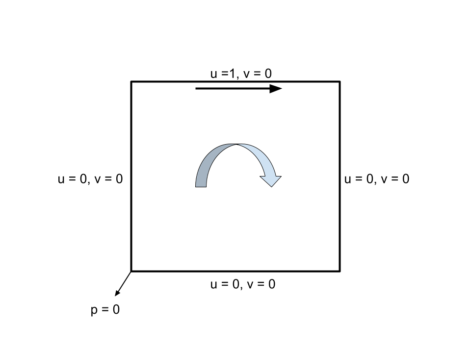
Figure 2: Lid Driven Cavity: An illustration of the computational domain and the associated boundary conditions.

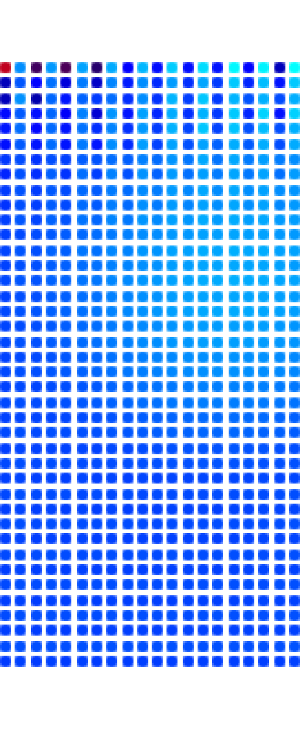
(a) Checkerboard pattern in pressure

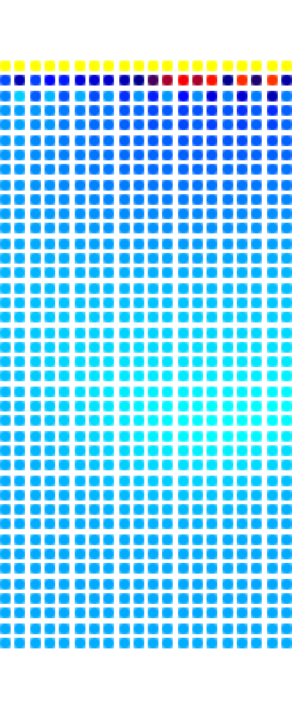
(b) Checkerboard pattern in $u$ (X-component of velocity)

Figure 3: Checkerboard pattern observed for $R_{e}=3200$.

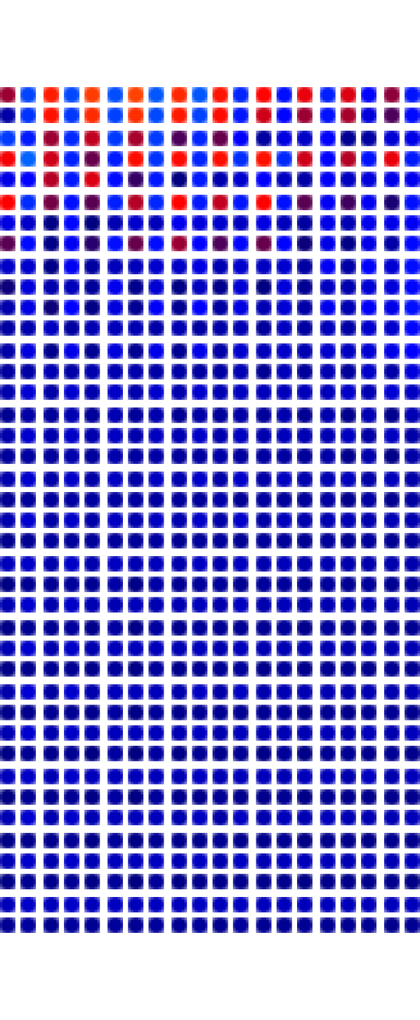
(a) Checkerboard pattern in pressure

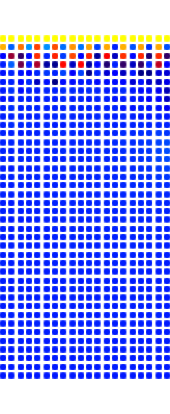
(b) Checkerboard pattern in $u$ (X-component of velocity)

Figure 4: Checkerboard pattern observed for $R_{e}=5000$.

3.3 Unsuccessful attempts to resolve the checkerboard problem in Eulerian GFDM

In order to resolve the problem, multiple prospective solutions were attempted as a part of this work. However, they do not alleviate the problem. For the sake of completeness of this work, these attempts are documented below, along with a brief explanation.

3.3.1 Upwinding/Downwinding the pressure term

In literature, there are references to one-sided differencing for the pressure derivatives to solve the issue of checkerboard patterns [12]. In the context of the present meshless method, the pressure derivative term was modified to replicate the one-sided difference.
The pressure gradient is re-written as

$$\nabla p|_{i}=2\hat{i}(\sum_{j\in S_{i}}C^{x}_{ij}p_{i-j})+2\hat{j}(\sum_{j\in S_{i}}C^{y}_{ij}p_{i-j})$$ (28)

where $\hat{i}$ and $\hat{j}$ are unit vectors in $x$ and $y$ directions respectively. The term $p_{i-j}$ is interpreted as the pressure at the mid-point between the points $i$ and $j$. The reconstruction of $p_{i-j}$ can incorporate upwinding/downwinding. For upwinding,

$$p_{i-j} = p_{i}\text{, if }\vec{V}_{i-j}\cdot(\vec{x_{j}}-\vec{x_{i}})>0$$ (29)

$$= p_{j}\text{, otherwise}$$ (30)

For downwindng, the above conditions are interchanged. However, both upwinding and downwinding do not solve the problem of checkerboarding. On the contrary, the solution is found to be unstable. This point needs a more detailed analysis and is outside the scope of the present work.

3.3.2 Varying the number of neighbours participating in the discretization

The number of points in the neighbourhood of a given point can be varied in a simulation. A larger neighbourhood of points would imply that the oscillations in pressure in the neighbourhood would be more visible and therefore, increases the chances of detection. Fig. 5(a) and (b) show the checkerboard patterns in pressure when number of neighbours is $15$ and $25$ respectively. It is evident that varying the number of neighbours does not resolve the issue of an oscillating field. In Sec. 3.4, we analyze why a regularly distributed neighbourhood is unable to detect oscillations in pressure. This explanation is equally valid for the cases of 15 and 25 neighbours.

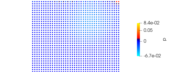
(a) Number of neighbours = 15

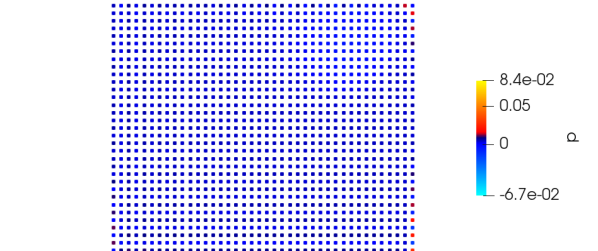
(b) Number of neighbours = 25

Figure 5: Checkerboard pattern observed for $R_{e}=3200$ for different number of neighbours.

3.3.3 Using a perturbed set of points

The motivation for this idea is that a uniform point cloud suffers the inadequacy in detecting checkerboard oscillations, as analysed in Sec. 3.4. The uniform point cloud was, thus, perturbed by a small random distance at all points such that the local neighbourhoods are no longer regular and symmetric. Unfortunately, this approach too does not solve the problem. Checkerboard oscillations in pressure emerge in the simulation, as shown in Fig. 6.

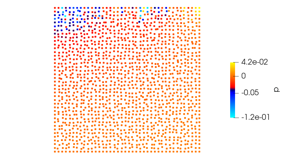
Figure 6: Pressure checkerboard pattern on an irregular point cloud.

It is likely that in this approach, the core problem of pressure checkerboarding still remains unaddressed due to the fact that the participation of a given point in the evaluation of the pressure derivative at that point, is minimal (although it may not be exactly zero).

3.4 Drawing parallels from mesh-based methods

The source of the checkerboard problem in mesh-based finite difference and finite volume methods is traced to the lack of participation of the point in consideration, in the evaluation of the pressure gradient at the same point. In other words, a hypothetical pressure field that oscillates between two distinct values ($p_{a}$ and $p_{b}$) from one point to the next, is still seen as a uniform pressure field since the pressure at the neighbouring points is the same.This is illustrated in Fig. 7.

$$\frac{\partial p}{\partial x}\Big{|}_{i}=\frac{p_{i+1}-p_{i-1}}{\Delta x}=0$$

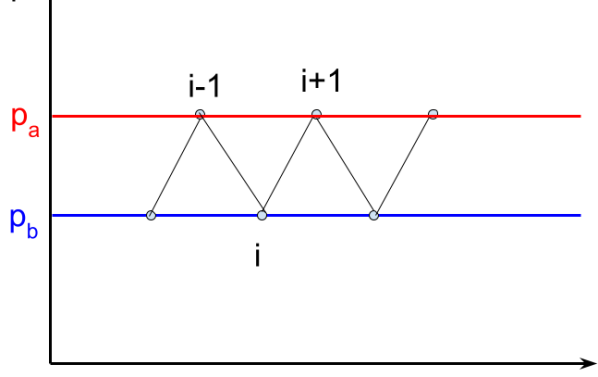
Figure 7: Pressure checkerboard pattern in 1-D; A central difference scheme for first derivative in pressure predicts zero pressure gradient.

In meshless methods, however, the neighbourhood of a point involves points that are not just in the immediate proximity, but also points that are farther away. Therefore, the hope is that the participation of these points in the estimation of the pressure gradient would make the checkerboard oscillations visible to the gradient operator and therefore, the oscillations would be suppressed. A regularly spaced neighbourhood of a point is shown in Fig. 8(a). The red and the blue colours indicate two distinct values between which pressure oscillates in the neighbourhood. The gradient operator is constructed at the point $P$. The numerical value of the differential operator, $C^{x}_{Pj}$,associated with each neighbour $j$, for the first derivative in $x$, is mentioned at corresponding locations in Fig. 8(b). It is evident from the values of the operator that neighbours that are positioned symmetrically w.r.t point $P$ have operators of the same magnitude and opposite sign. Evaluating the pressure gradient using these operators,

$$\frac{\partial p}{\partial x}\Big{|}_{P}=\sum_{j\in S_{p}}C^{x}_{Pj}p_{j}=p_{\text{red}}\sum_{\text{red}}C^{x}_{Pj}+p_{\text{blue}}\sum_{\text{blue}}C^{x}_{Pj}$$ (31)

This results in the two summations in the above equation to be zero. Therefore, using these operators in the computation of the derivative of pressure at $P$, would result in a zero pressure gradient, just as seen in mesh-based methods. In summary, although the oscillations in pressure are present in the neighbourhood of the point $P$, the operators do not detect the presence of the oscillations.

The two most well-known solutions to the problem of checkerboard oscillations in mesh-based methods are – (a) Staggered meshes and (b) Rhie-Chow interpolation. In staggered meshes, the pressure and the velocities are stored at different locations such that grid the formed by the pressure nodes is staggered w.r.t to the grid formed by the velocity nodes. The momentum equations are solved at the velocity nodes and the pressure gradient at these nodes is estimated from the pressure nodes that are staggered w.r.t the velocity node. Due to this, oscillations in pressure are detected by the system of equations, thus, solving the problem of checkerboarding. In the case of Rhie-Chow interpolation, collocated grids are used, where the pressure and velocity are stored at the same locations. The face velocities are estimated as the sum of the average of the velocities of the nodes that straddle the face and a correction term that depends on the third derivative of pressure at the face. This correction acts as a damping mechanism for any high frequency oscillations that may develop in the numerical solution[3].

In the context of meshless methods, these solutions are not straightforward to apply. Both the above solutions are designed in the context of finite-volume methods where a particular variable is solved for its cell-centred value and the fluxes at the cell faces are summed for each equation. Staggered meshes could correspond to staggered point clouds i.e. two sets of point clouds, one for pressure and another for velocity. For each point, two sets of differential operators will have to be computed. Evidently, the difficulty with this approach is that it dramatically increases memory requirements, number of operations and the amount of book-keeping required in a simulation. It also involves the generation of a staggered point cloud w.r.t a base point cloud, which could be non-trivial. Rhie-Chow interpolation, on the other hand, would require a solution to the integral form of the Navier-Stokes equations, which is the operating framework of the finite-volume method. In a meshless method like GFDM, the equations are solved in the differential form. Although, flux-based formulations can be used in GFDM as well, it relies on error minimization in flux derivatives rather than summing of fluxes over a control volume.

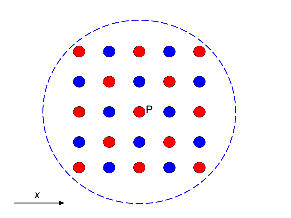
(a) An oscillating pressure field in the neighbourhood of a point

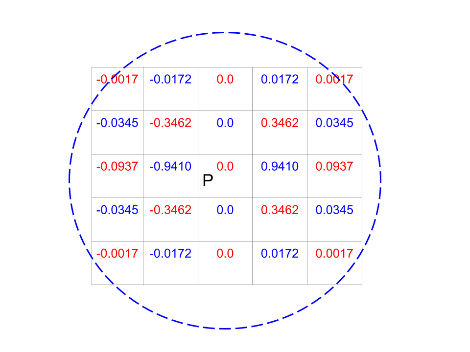
(b) The numerical values of the differential operators of the first derivative in $x$.

Figure 8: Checkerboard problem in meshless methods.

4 A solution: Point cloud adaptation

In this section, a point cloud adaption algorithm is described, which is effective in resolving the issue of checkerboard oscillations. The underlying idea is that the use of refined meshes/point clouds reduces the discretization errors to render an accurate numerical solution. One could employ a strategy of using a highly refined point cloud. However, there are two challenges with this approach – (a) the computational effort increases, (b) a priori estimate of the problematic regions is necessary. The point cloud adaptation algorithm presented here, identifies the regions of oscillations effectively and refines the point cloud only in such regions. This strategy, as presented in the Sec. 5, resolves the checkerboard problem with a only a small number of added points.

4.1 Error indicator

An error indicator based on the function value (in this case, pressure) is proposed. Using the procedure outlined in Sec. 2.2, an operator for the function approximation can be developed by setting

$$\vec{b}^{\text{ }T}=[1,0,0,0,0,0]$$ (32)

We denote the operator at a point $i$ with neighbouring points $j\in S_{i}$ as $C^{0}_{ij}$ such that the pressure from the weighted least squares approximation is given by

$$p_{i}=\sum_{j\in S_{i}}C^{0}_{ij}p_{n,j}$$ (33)

The error ($e$) is defined as

$$e_{i}=|p_{i}-p_{n,i}|$$ (34)

In this equation, $p_{n}$ is the pressure obtained from the numerical solution that contains the checkerboard oscillations. On the other hand, $p_{i}$ comes from a polynomial approximation of GFDM as shown in Eq. 33 and hence, will be a smooth function. As a result, the error $e_{i}$ will be high in regions where the checkerboard oscillations are prominent and low in other regions. This is pictorially illustrated in Fig. 9(a).

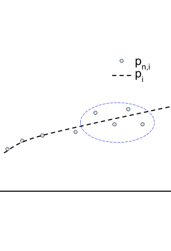
(a)

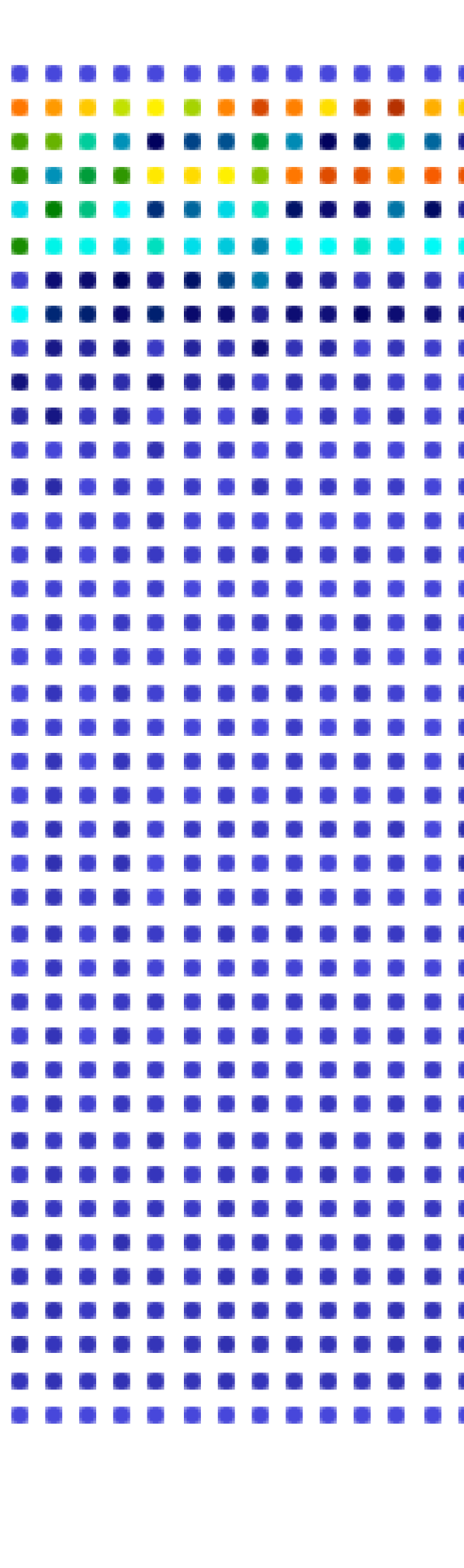
(b)

Figure 9: Error indicator: (a) An illustration showing the difference between the least squares fit ($p_{i}$) and the oscillating pressure field ($p_{n}$) (b) Error values in lid driven cavity problem for $R_{e}=3200$; large errors are seen in regions of checkerboard patterns.

Fig. 9(b) shows the error distribution in the lid driven cavity problem for $R_{e}=3200$; the corresponding pressure field is shown in Fig 3(a). It is seen that the error is high in regions of the checkerboard oscillations.
As a criteria for point cloud adaptation, we define

$$\psi_{i}=\frac{e_{i}}{e_{\text{max}}}$$ (35)

A threshold value of $\psi\geq 0.1$ is set in this work for point cloud adaptation.

4.2 Addition of points

The error indicator, as described in the previous section, is used as the criteria for adding points in the neighbourhood of a given point where the error is higher than the threshold. Consider the central point $i$ in Fig. 10.

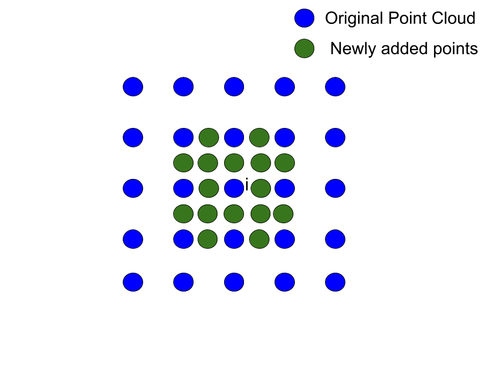
Figure 10: Point cloud adaptation: New points (green) are added to the existing point cloud (blue) in regions where the error exceeds the threshold.

The set of blue points are a part of the original point cloud. A new point is added at the mid-point between the point $i$ and each of its neighbours $j\in S_{i}$. Before the addition of a new point to the point cloud, the algorithm checks if there already exists a point at that location either from the original neighbourhood $S_{i}$ or an earlier adaptation at one of its neighbours $j$. A minimum distance criteria $d_{\text{min}}$ is set for the insertion of the new point such that the new point lies at least at $d_{\text{min}}$ from any of the existing points in the point cloud. This is done to ensure that the operators of GFDM, described in Sec. 2.2, are not unstable or singular.
The new point is initialized with the mean of the solution variables at the two points between which it is being inserted.

$$(u,v,p)_{\text{new}}=0.5[(u,v,p)_{i}+(u,v,p)_{j}]$$ (36)

4.3 Recalculation of neighbourhoods and differential operators

After the insertion of new points, the recalculation of the neighbourhood of points and differential operators is necessary. The adaptation of the point cloud would, in general, affect both the neighbourhood of points that have and have not participated in the adaptation procedure. Any change in neighbourhood would also result in the change in the differential operators. The advantage of using an Eulerian method is that estimation of neighbourhoods and differential operators need to be done only at the beginning of the simulation and whenever point cloud adaptation occurs. In Lagrangian methods, the points are continuously moving and would therefore, require these recalculations every time-step. The point cloud adaptation algorithm is summarized in Algorithm 1.

Algorithm 1 Point Cloud Adaptation

1:Estimtate the errors in the original point cloud using Eq. 34 and calculate $\psi_{i}\forall i$.

2:if $\psi_{i}\geq\psi_{\text{threshold}}$ then

3:     Flag the point $i$ for adaptation; $f_{i}=1$

4:     while $j$ in $S_{i}$ and $f_{j}\neq 1$ do

5:         Coordinates of new node, $\vec{R}_{\text{new}}=0.5(\vec{R}_{i}+\vec{R}_{j})$

6:         if $|\vec{R}_{\text{new}}-\vec{R}_{k}|\geq d_{\text{min}}$ $\forall k$ in the point cloud then

7:              Insert the new node

8:              Interpolate solution at the new node; Eq. 36.

9:         end if

10:     end while

11:end if

12:Recalculate neighbourhoods of points in the point cloud

13:Recalculate differential operators

5 Results

In this section, we present the commonly used benchmark flow, the lid driven cavity. Reynolds numbers of 3200 and 5000 are used and the checkerboarding patterns are reported for both Reynolds numbers. For each Reynolds number, the numerical solution is presented on two uniform sets of points and on an adapted set of points. The solutions on the adapted set of points are compared with the values reported in literature.

5.1 Lid Driven Cavity: $R_{e}=3200$

In this test case, the Reynolds number is set to $3200$. A test case with 1600 points (extracted from a regular $40\times 40$ grid) which exhibits checkerboard patterns, is used as reference. After the simulation is run for sometime on this base point cloud, the adaptation procedure is used to add points in regions of checkerboarding. The adapted point cloud is shown in Fig. 11.

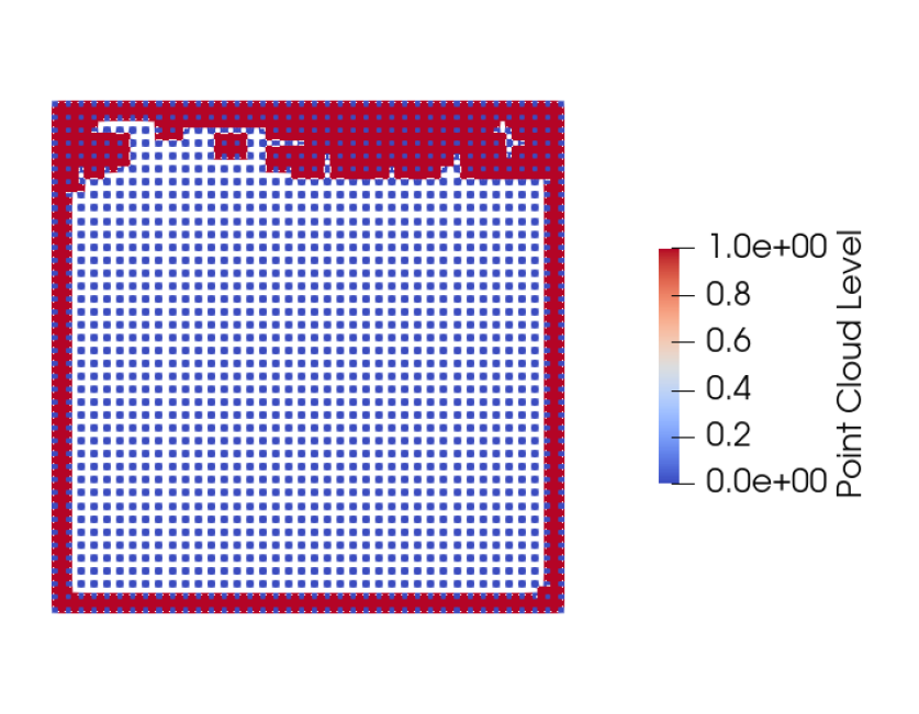
(a)

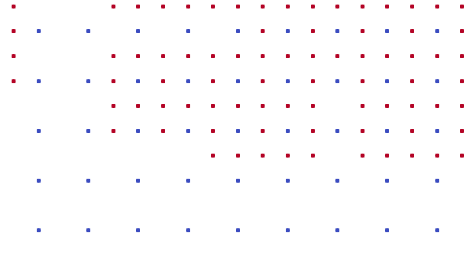
(b)

Figure 11: The adapted point cloud for $R_{e}=3200$: The red points denote the newly added points based on the error indicator values; (a) the entire point cloud, (b) a close-up view of the adapted point cloud.

The adapted point cloud contains 2585 points. For the sake of comparison of the extent of checkerboarding, we also use a finer uniform point cloud of 3600 points without adaptation(extracted from a regular $60\times 60$ grid). It is noted that the numerical results such as in Figs. 12 and 13 are presented here with the ’Delauney2D’ feature of Paraview that triangulates the point cloud before rendering the results. This method was preferred since it provides clearer visualization of the flow-field than using just points.
Figs. 12 and 13 show $p$ and $u$ contours on the three point clouds. While in the subfigures (a) and (b), the solution is on a uniform point cloud of 1600 and 3600 points, the subfigure (c) is on an adapted point cloud of 2585 points. It is noted that the checkerboard patterns in $p$ and $u$ are prominent in both the uniform point clouds, with the finer point cloud showing less oscillations. In comparison to both the uniform point clouds, the solution on the adapted point cloud is relatively smooth and manages to counter the checkerboard oscillations satisfactorily. It is also important to note that the adapted point cloud although has only 2585 points and it still performs better than a fine uniform point cloud of 3600 points.
In the cases with the checkerboard patterns, the solution stops changing after a certain point and converges to a non-physical solution. This can be observed in the streamline patterns of the converged solution in the three cases, as shown in Fig. 14. In Fig. 14(a) and (b), the solution on the uniform point cloud does not converge to form the secondary vortices despite sufficient number of points being present to resolve them as flow features. In Fig. 14(c), however, the adaptation of the point cloud suppresses the formation of spurious checkerboard oscillations and allows the solution to converge to the physically-correct solution. Fig. 15(a) reveals a good match in the $u$ velocity profile at the vertical mid-section with that of Ghia et al.[36].

(a)

(b)

(c)

Figure 12: Pressure contours for $R_{e}=3200$; (a) uniform point cloud of 1600 points, (b) uniform point cloud of 3600 points, (c) adapted point cloud of 2585 points.

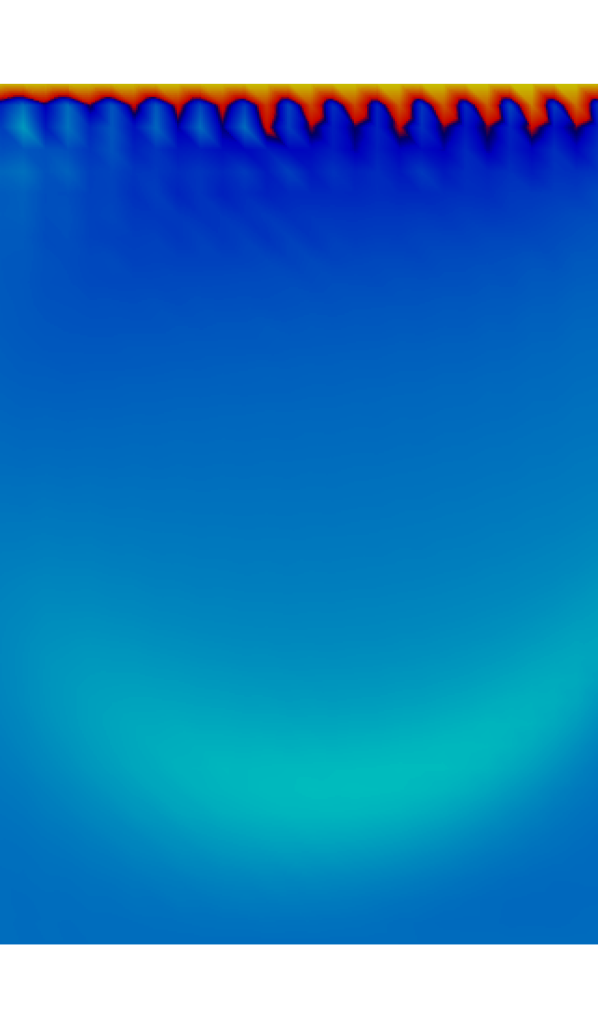
(a)

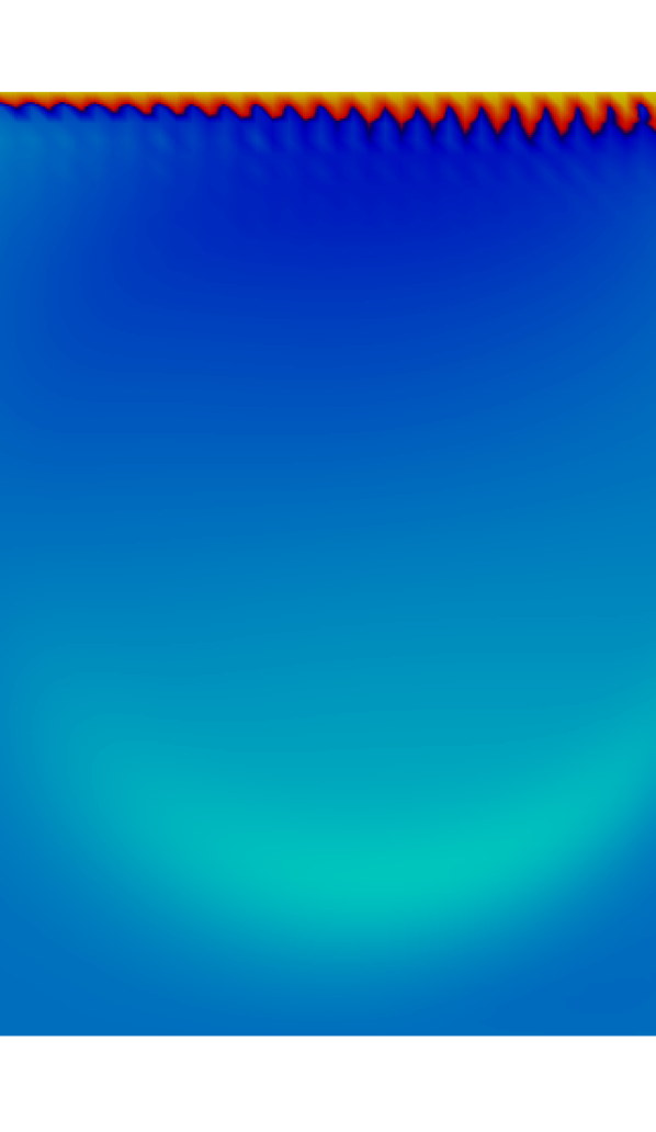
(b)

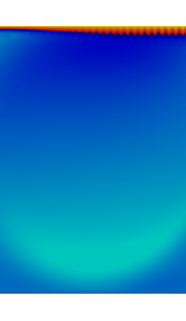
(c)

Figure 13: $u$ velocity contours for $R_{e}=3200$; (a) uniform point cloud of 1600 points, (b) uniform point cloud of 3600 points, (c) adapted point cloud of 2585 points.

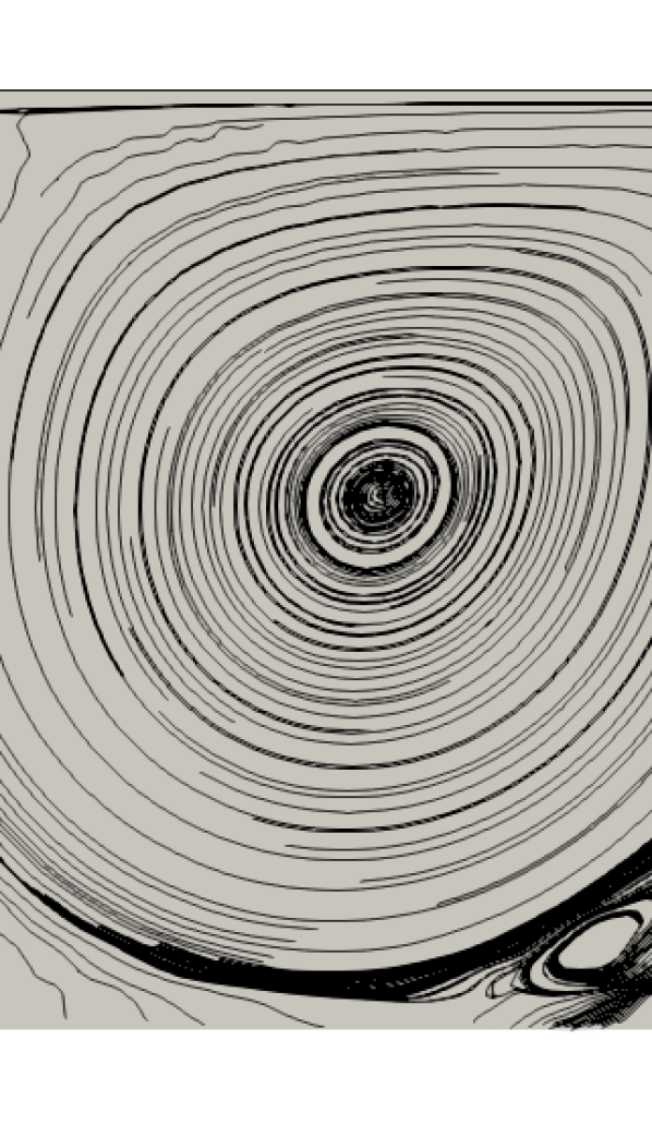
(a)

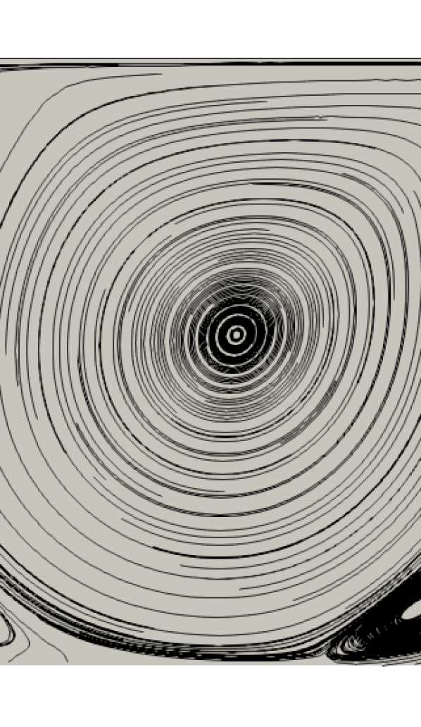
(b)

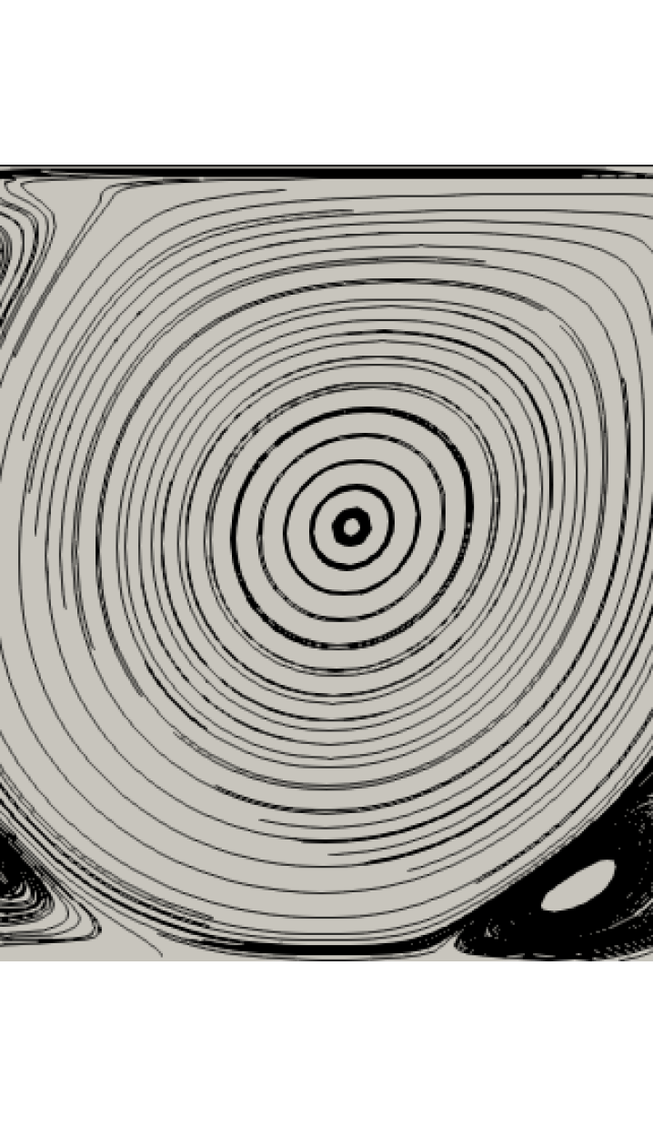
(c)

Figure 14: Streamlines for $R_{e}=3200$; (a) uniform point cloud of 1600 points, (b) uniform point cloud of 3600 points, (c) adapted point cloud of 2585 points. The secondary vortices develop only on the adapted point cloud.

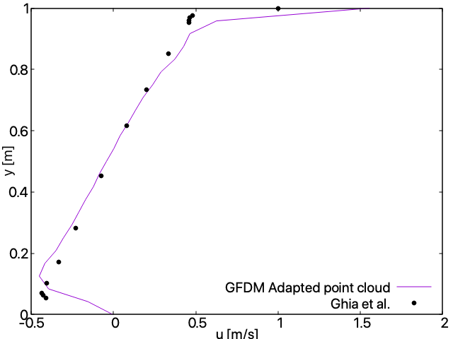
(a) $R_{e}=3200$

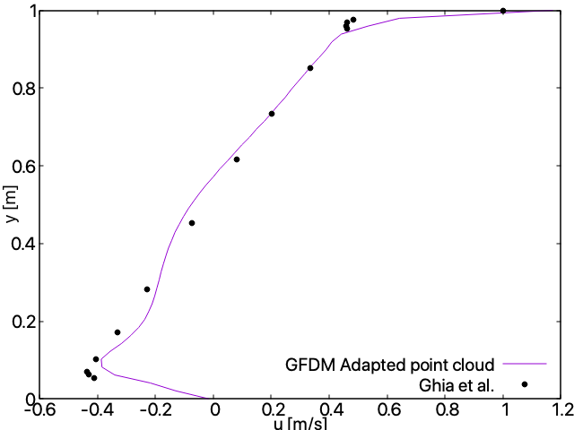
(b) $R_{e}=5000$

Figure 15: Comparison of $u$ velocity at the vertical mid-section, with literature

5.2 Lid Driven Cavity: $R_{e}=5000$

In this test case, the Reynolds number is set to $5000$. A test case with 3600 points (extracted from a regular $60\times 60$ grid) which exhibits checkerboard patterns, is used as reference. The adapted point cloud is shown in Fig. 16.

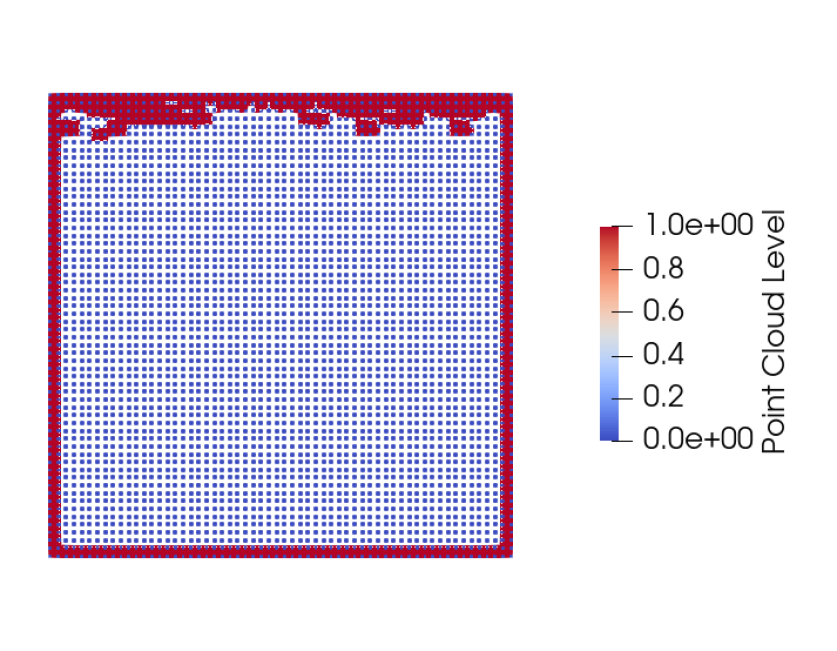
Figure 16: The adapted point cloud for $R_{e}=5000$: The red points denote the newly added points based on the error indicator values.

The adapted point cloud contains 4900 points. For the sake of comparison of the extent of checkerboarding, we also use a finer uniform point cloud of 4900 points without adaptation.
Figs. 17 and 18 show $p$ and $u$ contours on the three point clouds. While in the subfigures (a) and (b), the solution is on a uniform point cloud of 3600 and 4900 points, the subfigure (c) is on an adapted point cloud of 4900 points. It is noted that the checkerboard patterns in $p$ and $u$ are prominent in both the uniform point clouds. In comparison to the case of $R_{e}=3200$, the oscillations have a more severe effect on the convergence. This is evident in the $u$ contours in Fig. 18. The solutions on the uniform point clouds are far from the correct solution, which is obtained on the adapted point cloud (Fig. 18(c)).
In Fig. 19, the streamlines on the adapted point cloud show the formation of the secondary vortices. These features do not form on the uniform point clouds. Fig. 15(b) reveals a good match in the $u$ velocity profile at the vertical mid-section with that of Ghia et al.[36].

(a)

(b)

(c)

Figure 17: Pressure contours for $R_{e}=5000$; (a) uniform point cloud of 3600 points, (b) uniform point cloud of 4900 points, (c) adapted point cloud of 4900 points.

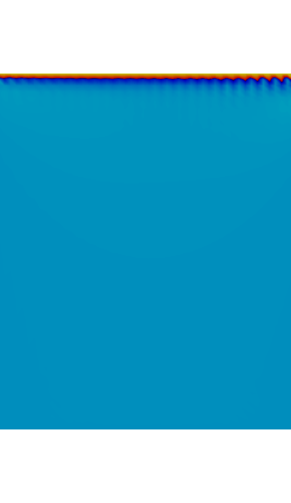
(a)

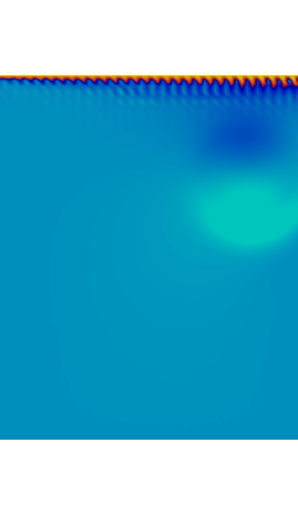
(b)

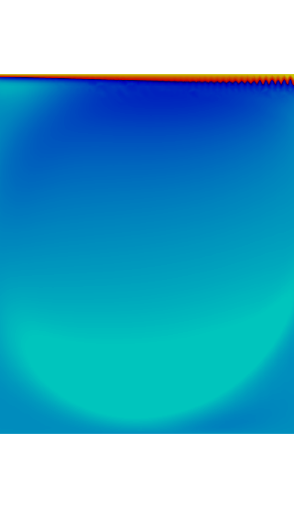
(c)

Figure 18: $u$ velocity contours for $R_{e}=5000$; (a) uniform point cloud of 3600 points, (b) uniform point cloud of 4900 points, (c) adapted point cloud of 4900 points.

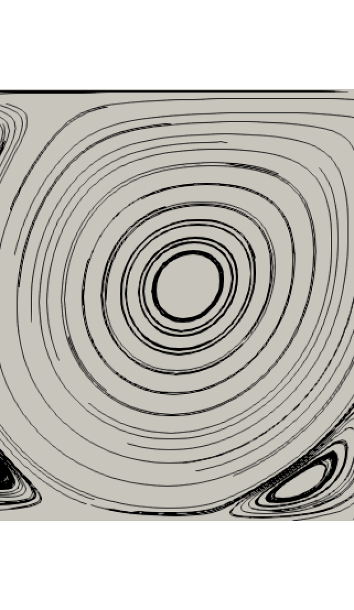
Figure 19: Streamlines for $R_{e}=5000$ on the adapted point cloud of 4900 points. The secondary vortices develop only on the adapted point cloud.

6 Conclusions

This paper discusses the checkerboard patterns emerging in an Eulerian meshless numerical solution to the incompressible Navier-Stokes equations. The primary aim of the work is to bring to notice the persistence of this problem in meshless numerical frameworks, which is less frequently reported or discussed. The work lists a few unsuccessful attempts to resolve the checkerboard problem. The method of point cloud adaptation works best in resolving the problem due to the ability of the algorithm to detect regions of checkerboard oscillations and add points in these regions to resolve the flow better. This method offers an advantage in terms of retaining the simplicity of the projection method to solve the Navier-Stokes equations without performing any special interpolations that are easier performed in mesh-based methods. Another advantage this method offers is that the adaptation of the point cloud is very easily incorporated into the meshless framework since no re-meshing needs to be done. The point cloud adaptation method is tested on the lid driven cavity problem of high $R_{e}$ and is seen that the solution converges to the physically correct one, with adaptation. Without adaptation, the solution exhibits checkerboard oscillations and in many cases, does not allow the numerical solution to converge to the physically correct values. The adaptation algorithm adds only points to critical regions of a point cloud on which checkerboarding occurs and as a result, can generate correct solutions with a small number of added points. This makes it computationally more efficient than a priori refinement of the point cloud.

References

- [1] Suhas V Patankar and D Brian Spalding. A calculation procedure for heat, mass and momentum transfer in three-dimensional parabolic flows. In Numerical prediction of flow, heat transfer, turbulence and combustion, pages 54–73. Elsevier, 1983.
- [2] Chae M Rhie and Wei-Liang Chow. Numerical study of the turbulent flow past an airfoil with trailing edge separation. AIAA journal, 21(11):1525–1532, 1983.
- [3] Joel H Ferziger and Milovan PeriC. Computational methods for fluid dynamics, 2002.
- [4] S Majumdar. Role of underrelaxation in momentum interpolation for calculation of flow with nonstaggered grids. Numerical heat transfer, 13(1):125–132, 1988.
- [5] TF Miller and FW Schmidt. Use of a pressure-weighted interpolation method for the solution of the incompressible navier-stokes equations on a nonstaggered grid system. Numerical Heat Transfer, Part A: Applications, 14(2):213–233, 1988.
- [6] YG Lai, RMC So, and AJ Przekwas. Turbulent transonic flow simulation using a pressure-based method. International journal of engineering science, 33(4):469–483, 1995.
- [7] Ismet Demirdžić and Samir Muzaferija. Numerical method for coupled fluid flow, heat transfer and stress analysis using unstructured moving meshes with cells of arbitrary topology. Computer methods in applied mechanics and engineering, 125(1-4):235–255, 1995.
- [8] Paul Bartholomew, Fabian Denner, Mohd Hazmil Abdol-Azis, Andrew Marquis, and Berend GM van Wachem. Unified formulation of the momentum-weighted interpolation for collocated variable arrangements. Journal of Computational Physics, 375:177–208, 2018.
- [9] AW Date. Solution of navier-stokes equations on non-staggered grid. International journal of heat and mass transfer, 36(7):1913–1922, 1993.
- [10] AW Date. Complete pressure correction algorithm for solution of incompressible navier-stokes equations on a nonstaggered grid. Numerical Heat Transfer, 29(4):441–458, 1996.
- [11] AW Date. Fluid dynamical view of pressure checkerboarding problem and smoothing pressure correction on meshes with colocated variables. International journal of heat and mass transfer, 46(25):4885–4898, 2003.
- [12] Marcelo Reggio and Ricardo Camarero. Numerical solution procedure for viscous incompressible flows. Numerical Heat Transfer, Part A: Applications, 10(2):131–146, 1986.
- [13] GD Thiart. Finite difference scheme for the numerical solution of fluid flow and heat transfer problems on nonstaggered grids. Numerical Heat Transfer, 17(1):43–62, 1990.
- [14] Zineb Tabbakh, Mohammed Seaid, Rachid Ellaia, Driss Ouazar, and Fayssal Benkhaldoun. A local radial basis function projection method for incompressible flows in water eutrophication. Engineering Analysis with Boundary Elements, 106:528–540, 2019.
- [15] Zineb Tabbakh, Rachid Ellaia, and Driss Ouazar. Application of a local meshless modified characteristic method to incompressible fluid flows with heat transport problem. Engineering Analysis with Boundary Elements, 134:612–624, 2022.
- [16] Shantanu Shahane and Surya Pratap Vanka. A semi-implicit meshless method for incompressible flows in complex geometries. Journal of Computational Physics, 472:111715, 2023.
- [17] YVSS Sanyasiraju and G Chandhini. Local radial basis function based gridfree scheme for unsteady incompressible viscous flows. Journal of Computational Physics, 227(20):8922–8948, 2008.
- [18] Ali Rahmani Firoozjaee and Mohammad Hadi Afshar. Steady-state solution of incompressible navier–stokes equations using discrete least-squares meshless method. International Journal for Numerical Methods in Fluids, 67(3):369–382, 2011.
- [19] Tobias Seifarth. Numerische Algorithmen für gitterfreie Methoden zur Lösung von Transportproblemen. BoD–Books on Demand, 2022.
- [20] S Majid Hosseini and James J Feng. Pressure boundary conditions for computing incompressible flows with sph. Journal of Computational physics, 230(19):7473–7487, 2011.
- [21] Amir Zainali, Nima Tofighi, M Safdari Shadloo, and M Yildiz. Numerical investigation of newtonian and non-newtonian multiphase flows using isph method. Computer Methods in Applied Mechanics and Engineering, 254:99–113, 2013.
- [22] Sharen J Cummins and Murray Rudman. An sph projection method. Journal of computational physics, 152(2):584–607, 1999.
- [23] Ashkan Rafiee and Krish P Thiagarajan. An sph projection method for simulating fluid-hypoelastic structure interaction. Computer Methods in Applied Mechanics and Engineering, 198(33-36):2785–2795, 2009.
- [24] Joe J Monaghan. Simulating free surface flows with sph. Journal of computational physics, 110(2):399–406, 1994.
- [25] Prabhu Ramachandran and Kunal Puri. Entropically damped artificial compressibility for sph. Computers & Fluids, 179:579–594, 2019.
- [26] Pratik Suchde, Jörg Kuhnert, and Sudarshan Tiwari. On meshfree gfdm solvers for the incompressible navier–stokes equations. Computers & Fluids, 165:1–12, 2018.
- [27] Sudarshan Tiwari and Jörg Kuhnert. Finite pointset method based on the projection method for simulations of the incompressible navier-stokes equations. In Meshfree methods for partial differential equations, pages 373–387. Springer, 2003.
- [28] Sudarshan Tiwari and Jörg Kuhnert. Modeling of two-phase flows with surface tension by finite pointset method (fpm). Journal of computational and applied mathematics, 203(2):376–386, 2007.
- [29] Anthony Jefferies, Jörg Kuhnert, Lars Aschenbrenner, and Uwe Giffhorn. Finite pointset method for the simulation of a vehicle travelling through a body of water. In Meshfree methods for partial differential equations VII, pages 205–221. Springer, 2015.
- [30] Mohammad R Hashemi, Mehrdad Taghizadeh Manzari, and Rouhollah Fatehi. Evaluation of a pressure splitting formulation for weakly compressible sph: Fluid flow around periodic array of cylinders. Computers & Mathematics with Applications, 71(3):758–778, 2016.
- [31] R Fatehi and MT Manzari. A remedy for numerical oscillations in weakly compressible smoothed particle hydrodynamics. International Journal for Numerical Methods in Fluids, 67(9):1100–1114, 2011.
- [32] JL Cercos-Pita, RA Dalrymple, and A Herault. Diffusive terms for the conservation of mass equation in sph. Applied Mathematical Modelling, 40(19-20):8722–8736, 2016.
- [33] Alexandre Joel Chorin. Numerical solution of the navier-stokes equations. Mathematics of computation, 22(104):745–762, 1968.
- [34] Benjamin Seibold. M-Matrices in meshless finite difference methods. Shaker, 2006.
- [35] Pratik Suchde. Conservation and accuracy in meshfree generalized finite difference methods. Kaiserslautern University of Technology, Germany, 2018.
- [36] UKNG Ghia, Kirti N Ghia, and CT Shin. High-re solutions for incompressible flow using the navier-stokes equations and a multigrid method. Journal of computational physics, 48(3):387–411, 1982.