Reinforcing POD-based model reduction techniques in reaction-diffusion complex networks using stochastic filtering and pattern recognition

Abstract

Complex networks are used to model many real-world systems. However, the dimensionality of these systems can make them challenging to analyze. Dimensionality reduction techniques like POD can be used in such cases. However, these models are susceptible to perturbations in the input data. We propose an algorithmic framework that combines techniques from pattern recognition (PR) and stochastic filtering theory to enhance the output of such models. The results of our study show that our method can improve the accuracy of the surrogate model under perturbed inputs. Deep Neural Networks (DNNs) are susceptible to adversarial attacks. However, recent research has revealed that Neural Ordinary Differential Equations (neural ODEs) exhibit robustness in specific applications. We benchmark our algorithmic framework with the neural ODE-based approach as a reference.

Keywords: Stochastic filtering $\cdot$ Pattern Recognition (PR) $\cdot$ Dimensionality reduction $\cdot$ Dynamical systems

1   Introduction

Complex networks offer valuable insights into real-world systems, including the spread of epidemics ([1]) and the understanding of biochemical and neuronal processes described in [2]. However, the computational complexity in modelling such systems arises when dealing with large state spaces. To address this challenge, methods like Proper Orthogonal Decomposition (POD) ([3]) are employed to capture patterns while operating in reduced dimensions. Nevertheless, the sensitivity of these methods to data poses a significant issue. Consequently, the question arises regarding how to enhance a surrogate model obtained from POD to accommodate perturbed data sets. This study provides insights into this question specifically for reaction-diffusion-based complex systems.

In the context of dynamical systems, the surrogate model serves as an approximation to capture the discrepancies between the model and the true state, where the real-world system is often modelled by ODEs or PDEs. The underlying process may not be effectively captured because of a lack of understanding of the system. Several machine learning (ML) methods have been explored to construct surrogate models for low-order chaotic systems. These methods include analogs ([4]), recurrent neural networks ([5], [6]), residual neural networks representing resolvents ([7], [8]) or the underlying differential equations such as ODEs ([9], [10], [11], [12]).

Notably, the study in [7] demonstrates the combination of ML and data assimilation (DA) to address the issue of sparse observations. However, the computational cost of the DA step remains a significant consideration. Other efforts to correct model error involve using weak-constraint DA methods, as described in [13]. Moreover the study in [14] proposes an ML-DA framework for correcting model errors.

Contributions of our paper: In our study, we propose a novel framework to enhance POD-based model reduction techniques in reaction-diffusion-based complex systems. We use stochastic filtering theory to estimate and account for errors by leveraging patterns of errors observed in known state transitions. Updates in the filtering step are done using a sparse graph obtained by reweighting of edges using a dynamic optimization framework.

The key steps used in the framework are as follows. Initially, we utilize a dynamic optimization framework (step 1 in Section 3.2) to extract a sparse graph from known snapshots of solution trajectories. The primary motivation behind this step is that when we employ the filtering step (step 3 in Section 2) to the reduced order model (ROM) of the given reaction-diffusion system, as the timestep progresses, we may need to make intermittent updates to the system variables, so we propose to use a sparse approximation to the given graph to make the updates. Subsequently, the deviations between the ROM and the actual trajectories are obtained, organizing these deviations into clusters, forming the basis of our subsequent analysis.

We employ the adjoint sensitivity method to ascertain the weights governing the transitions between distinct clusters (see Section 2b). By exploring available known patterns of state transitions with the Markovian assumption, we can effectively assign appropriate weights.
Getting optimal states from noisy measurements with the surrogate forward model forms the core of the filtering problem. The particle filtering technique is utilized to generate the reaction-diffusion state vector at various time steps with measurements taken from ROM.

The article is organized as follows; we begin by discussing the orthogonal collocation method on finite elements which is an integral part of the dyanamic optimization framework (Section 3.2) to produce sparse graph. We then give a brief motivation of understanding spatiotemporal patterns in complex networks by providing certain examples (Section 1.2). The POD method for solving initial-value problem is discussed briefly (Section 2). Certain bounds are obtained for the linear case of diffusion by utilizing existing literature. The methodology of the framework is illustrated in detail (Theorems 2, 3), presenting the underlying dynamic optimization problem for the linear case of diffusion as well as the nonlinear reaction-diffusion system. Empirical results are presented next, see Section 5. Benchmarking of the framework is done with the neural ODENet method as the baseline (Section 6).

1.1   Orthogonal collocation method on finite elements

The orthogonal collocation method is a widely adopted numerical technique for efficiently solving differential equations, particularly in dynamic optimization problems. It offers a versatile solution for both ordinary and partial differential equations. Please refer to ([15], [16]) to know more about the method.

The proposed method entails partitioning the problem domain into a discrete set of collocation points, ensuring that the polynomial approximation of the vector field $f(t,z(t))$ satisfies the orthogonality condition, Some choices for collocation points include Legendre, Chebyshev, and Gaussian points.

By ensuring that the differential equations hold true at the collocation points, a system of algebraic equations is formulated. This system of algebraic equations can be solved through various numerical techniques, such as Newton’s method or direct solvers, yielding an approximate solution to the original differential equations. It is important to note that the selection of collocation points and basis functions has a significant influence on the accuracy and efficiency of the method. To illustrate this aspect, we provide an example in Figure 1 using the Lotka-Volterra system.

$$\frac{dx}{dt} =\alpha x-\beta xy$$

$$\frac{dy}{dt} =\delta xy-\gamma y.$$

Here $x$ and $y$ denote the prey and predator population. The parameters $\alpha,\beta$ determine the prey growth rate and $\delta,\gamma$ determine the predator growth rate.

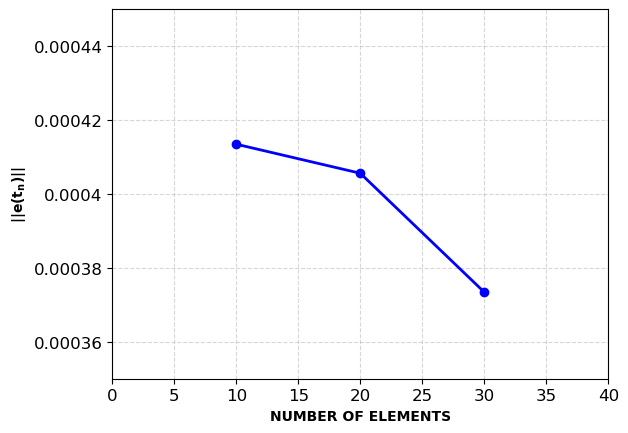
Figure 1: Error observed at the endpoint when modifying the number of collocation elements applied to the Lotka-Volterra system.

1.2   Spatio temporal propogation in graphs

Investigating spatiotemporal propagation in complex networks has gained considerable interest across multiple disciplines, such as physics, biology, and neuroscience. Complex networks consist of interconnected nodes, and the interactions between these nodes lead to dynamic processes. Unravelling the mechanisms of information, phenomena, or dynamics propagation within these networks is vital for comprehending the intricate behaviours and emergent characteristics of interconnected systems.

Spatio-temporal propagation refers to the transmission or diffusion of information, signals, or dynamics throughout the interconnected nodes and edges of a complex network. It encompasses the examination of how localized events, disturbances, or modifications in one section of the network can disseminate, develop, and influence other nodes or regions within the network. Investigating spatiotemporal propagation has significant implications in diverse fields (Hens, 2019). We highlight a few examples where complex networks find application.

1. Epidemic Spread $(\mathbb{E})$: Understanding how infectious diseases propagate through social networks can aid in designing effective strategies for disease control, information dissemination, or opinion information. The SIS(susceptible-infected-susceptible) model used to study epidemic spreading is given below,

   $$\frac{dx_{i}}{dt}=-x_{i}+\sum_{j=1}^{N}A_{ij}(1-x_{i})x_{j}.$$

   $A_{ij}$ represents the $(i,j)$-th entry of the adjacency matrix of the graph. $N$ denotes the number of nodes.

2. Diffusion Processes  $(\mathbb{D})$: Investigating diffusion phenomena, such as heat transfer and molecular diffusion, help in modelling and optimizing processes that involve spreading or transport. If we consider the normalized Laplacian matrix of the graph, we could get the equivalent discrete dynamical system for the heat equation. Normalized Laplacian matrix $\mathcal{L}=D^{-1/2}LD^{-1/2}$, where $D$ is the diagonal matrix of degrees and $L=D-A$ is the Laplacian matrix of the graph.

   $$\frac{du}{dt}=-\mathcal{L}u,\;\;$$

   Here $u\in\mathbb{R}^{n},u(x,t)$ denotes the temperature at node $x$ and time $t$.

3. Neural Dynamics ($\mathbb{N}$): Studying the spread of neural activity within brain networks offers valuable insights into cognition and various brain disorders. One such system as mentioned in [17] is described below,

   $$\frac{dx_{i}}{dt}=-Bx_{i}+C\tanh{x_{i}}+\sum_{j=1}^{N}A_{ij}\tanh{x_{j}}.$$

2   Proper Orthogonal Decompostion for Dynamical systems

In this section we give a brief description on how we could use POD in the case of initial value problems for dynamical systems. Given a dataset $\mathcal{D}$ consisting of a collection of points $x^{c}_{i}$, where $x^{c}_{i}\in\mathbb{R}^{n}$ denote the state of the system at time $t_{i}$ for a particular trajectory $c$, the POD method seeks a subspace $S\subset\mathbb{R}^{n}$ such that

$$||\mathcal{D}-\rho_{S}\mathcal{D}||^{2}$$

is minimized. $\rho_{S}$ is the orthogonal projection onto the subspace $S$ and $\rho_{S}\mathcal{D}$ denotes the projected data set.

$S\subset\mathbb{R}^{n}$ is the best $k$ dimensional approximating affine subspace, with the matrix $\rho$ of projection consisting of leading $k$ eigenvectors of the covariance matrix ($\bar{R}$). The subspace for a particular data set $\mathcal{D}$ is uniquely determined by projection matrix $P$ and mean $\bar{x}$, $P=\rho^{T}\rho$.

$$\bar{R} =\sum_{c=1}^{N_{T}}\int_{0}^{T}(x^{c}(t)-\bar{x})(x^{c}(t)-\bar{x})^{T}dt$$

$$\bar{x} =\frac{1}{N_{T}T}\sum_{c=1}^{N_{T}}\int_{0}^{T}x^{c}(t)dt.$$

$N_{T}$ denotes the number of trajectories. The initial value problem is to be solved is from time $t=0$ to $t=T$.

Asymptotic analysis of the advantages of POD and their sensitivity analysis is done in [3]. Let us consider a dynamical system in $\mathbb{R}^{n}$ given by a vector field $f$,

$$\dot{x}=f(x,t).$$

The ROM vector field will be given by

$$\dot{z}=\rho f(\rho^{T}z+\bar{x},t)=f_{a}(z,t).$$

Thus an initial value problem for the system $\dot{x}=f(x,t)$ with $x(0)=x_{0}$ using the projection method is given by

$$\dot{\hat{x}}=Pf(\hat{x},t);\;\;\hat{x}(0)=\hat{x}_{0}=P(x_{0}-\bar{x})+\bar{x}.$$ (1)

Here $\hat{x}_{0}$ is the projection of $x_{0}$ onto the subspace $S$.
Proposition: (Rathinam and Petzold [3]) Consider applying POD to a data set $\mathcal{D}$ to find the best approximating $k(<n)$ dimensional subspace. Let the ordered eigenvalues of the covariance matrix of the data $\mathcal{D}$ be given by $\lambda_{1}\geq\cdots\geq\lambda_{n}$. Suppose $\lambda_{k}>\lambda_{k+1},$ which ensures that $P(\mathcal{D})$ is well defined. Then

$$S_{k}(\mathcal{D})=\text{max}_{i\leq k,j\leq n-k}\,\sqrt{2}\;\frac{\sqrt{\lambda_{i}+\lambda_{j+k}}}{\lambda_{i}-\lambda_{j+k}}\sqrt{\lambda_{1}+\cdots+\lambda_{n}}\geq\sqrt{2}.$$ (2)

3   Problem statement

The sensitivity of the projection matrix $\rho$ to the underlying data set $\mathcal{D}$ is given by the expression in Equation (2). The implication is that when faced with a new random initial condition, approximating the trajectory through a discretization scheme based on the POD formulation of the complex system, as previously discussed, may overlook the deviations from the true state.

$$x_{k+1} =M(\hat{x}_{k})+e_{mh}(t_{k+1})+e_{ml}(t_{k+1})$$

$$z_{k} =\rho(x_{k}-\bar{x})+e_{oh}(t_{k})+e_{ol}(t_{k})$$

Here $x_{k+1}$ denotes the true state of the system and $\hat{x}_{k}$ denotes the approximate solution from POD, $M(\cdot)$ denotes the discretization used for the system (Eq. 1), for example if the Euler forward scheme is used, we get $M(\hat{x}_{k})=\hat{x}_{k}+hPf(\hat{x}_{k},t_{k})$, where $h$ denotes the step size. $e_{mh}(t_{k+1}),e_{ml}(t_{k+1})$ denotes the high and low wavelength component of error that captures deviations between the true state and state obtained from ROM (Eq. 1) at time $t_{k+1}$. $e_{oh}(t_{k}),e_{ol}(t_{k})$ denotes the high and low wavelength components of error which captures difference between the measurement and state at time $t_{k}$.

We present a framework that captures the uncertainties arising from the sensitivities in the POD matrix $\rho$ for generating comparable dynamics to the full model in reaction-diffusion complex networks when utilizing the ROM.

3.1   Linear dynamical system involving graphs

We first evaluate our framework for the case of linear dynamical system on graphs.

We consider the following linear dynamical system involving the Laplacian matrix of a graph,

$$\frac{dF(x,t)}{dt}=-LF(x,t).$$

where $F(x,t)$ denotes the solution at node $x$ and time $t$.

Existing techniques used for approximating such linear systems are [18], [19], and [20]. We transfer existing results to the dynamic optimization framework (Section 3.2). From the existing literature, we obtain lower and upper bounds on the degrees of the graph. Bounds on the weights of edges of the spectral approximation of the graph are also obtained in this section.

The work in [20] focuses on creating spectral sparsifiers wherein edges are sampled based on the resistance of an edge $R_{e}$, $p_{e}$ is the probability with which edge $e$ is sampled where $p_{e}=\frac{w_{e}R_{e}}{(n-1)}$, and $R_{e}=||L^{1/2}L_{e}L^{1/2}||$, see Algorithm 3.1. Effective resistance $R_{e}$ is difficult to compute, and a much easier parameter to compute is given by the edge connectivity ($k_{e}$). $k_{e}\geq max(\frac{1}{R_{e}},s_{e})$ where $s_{e}$ denotes the edge strength. Thus from these relations, we can see that

$$\frac{w_{e}}{p_{e}}=\frac{(n-1)}{R_{e}}\leq(n-1)k_{e}.$$

Algorithms to compute individual edge connectivity of the graphs with $O(|V||E|)$ time complexity are discussed in [21].

$$H=\textbf{Sparsify}(G,q)\cite[cite]{[\@@bibref{}{spielman2009graph}{}{}]}$$

Choose a random edge of with probability proportional to ,

and add to with weight . Take samples independently

with replacement, summing weights if an edge is chosen more than once.

The following lemma specifies certain bounds which is based on Algorithm 3.1.

Lemma 1.

[22] Suppose we sample $q>\frac{4n\log{n}}{\beta}$ edges of $G$ as in Sparsify with probabilities that satisfy

$$p(u,v)\geq\frac{\beta}{n\text{min(deg(u), deg(v))}}$$

for some constant $0<\beta<1$. Then with probability atleast $1-\frac{1}{n}$,

$$\sum_{e\ni v}\frac{\tilde{w}_{e}}{w_{e}}\leq 2\text{deg(v)}\;\;\;\forall\;v\in V.$$

Getting bounds on all the weights of the edges of the approximation of the graph $H$ based on the properties of effective resistances or the local edge connectivities of an edge can be computationally demanding. Thus, we focus on obtaining these bounds through concentration inequalities ([23]).

Theorem 1.

Bernstein’s Inequality: Suppose $X_{1},\ldots,X_{n}$ are independent random variables with finite variances, and suppose that $\text{max}_{1\leq i\leq n}|X_{i}|\leq B$ almost surely for some constant $B>0$. Let $V=\sum_{i=1}^{n}\mathbb{E}X_{i}^{2}.$ Then, for every $t\geq 0,$

$$P\{\sum_{i=1}^{n}(X_{i}-\mathbb{E}X_{i})\geq t\}\leq exp\bigg{(}-\frac{t^{2}}{2(V+tB/3)}\bigg{)}$$

and

$$P\{\sum_{i=1}^{n}(X_{i}-\mathbb{E}X_{i})\leq-t\}\leq exp\bigg{(}-\frac{t^{2}}{2(V+tB/3)}\bigg{)}$$

Theorem 2.

If we sample each edge (u,v) of a graph with probabilities $p_{uv}\propto R_{uv}$, where $p_{uv}\geq\frac{\beta}{n\text{min(deg(u), deg(v))}}$, then $\mathbb{P}\{\frac{\sum_{i=1}^{q}X_{i}}{q}-w_{uv}\geq t\}\leq\frac{1}{mn}$, $t\geq\frac{\epsilon_{1}c_{1}}{3q}+\sqrt{\frac{2\epsilon_{1}w_{uv}c_{1}}{q}+(\frac{\epsilon_{1}c_{1}}{3q})^{2}}$, where

$$X_{i}=\left\{\begin{array}[]{ll}\begin{array}[]{l}\frac{w_{uv}}{p_{uv}},\text{\;\;with probability $p_{uv}$ (u,v) $\in\;E(G)$}\\ \\ 0,\text{\;\;otherwise.}\\ \\ \end{array}&\end{array}\right.$$

$\epsilon_{1}=\log(nm),|X_{i}|\leq c_{1},c_{1}=\frac{w_{uv}nc_{2}}{\beta}$, where $c_{2}=\text{min(deg($u$), deg($v$))}$.

Proof.

The Expectation $\mathbb{E}[X_{i}]=w_{uv}$,

$$\sum_{i=1}^{q}\mathbb{E}(X_{i}^{2})=q\frac{w_{uv}^{2}}{p_{uv}}\leq\frac{w_{uv}^{2}\,n\,c_{2}\,q}{\beta},\;\text{where $c_{2}=\text{min(deg($u$), deg($v$))}$}$$

Let $c_{1}=\frac{w_{uv}nc_{2}}{\beta}$, it can observed that $|X_{i}|\leq c_{1}.$
Applying the Bernstein’s Inequality we get

$$\mathbb{P}\bigg{\{}\frac{\sum_{i=1}^{q}X_{i}}{q}-w_{uv}\geq t\bigg{\}}\leq\exp{\bigg{(}-\frac{(tq)^{2}}{2}\frac{1}{(w_{uv}c_{1}q+\frac{c_{1}tq}{3})}\bigg{)}}$$

$$\frac{(tq)^{2}}{2}\frac{1}{(w_{uv}c_{1}q+\frac{c_{1}tq}{3})}\geq\log{nm}\equiv\epsilon_{1}$$

Completing the squares we get,

$$(t-\frac{\epsilon_{1}c_{1}}{3q})^{2}\geq\frac{2\epsilon_{1}w_{uv}c_{1}}{q}+(\frac{\epsilon_{1}c_{1}}{3q})^{2}$$

$$\text{Thus\;\;}t\geq\frac{\epsilon_{1}c_{1}}{3q}+\sqrt{\frac{2\epsilon_{1}w_{uv}c_{1}}{q}+(\frac{\epsilon_{1}c_{1}}{3q})^{2}}\text{\;\;\;will suffice.}$$

∎

Notation: Let $G$ be a weighted graph that is simple, meaning it does not contain any self-loops or multiple edges. We define two sets of vertices based on their degrees in $G$. The set $l_{m}$ consists of the $n-m+1$ vertices with the largest degrees in $G$, while the set $s_{m}$ consists of the $m$ vertices with the smallest degree in $G$. We then create two subgraphs, denoted as $G_{l_{m}}$ and $G_{s_{m}}$, by taking the subsets of $G$ induced by the vertices in $l_{m}$ and $s_{m}$ respectively. $l_{i}=\{v_{i},v_{i+1},....,v_{n}\}$ and $s_{i}=\{v_{1},v_{2},...,v_{i}\}$. Let the upper bound for maximal weight for sparsified graph be $a_{ub}$ and upper bound for the largest degree of subgraph $G_{l_{i}}$ be given by $\Delta(G_{l_{i}})_{ub}$ and smallest degree of subgraph $G_{s_{i}}$ be given by $\delta(G_{s_{i}})_{lb}$. Here $d_{v_{1}}\leq d_{v_{2}}\leq\ldots\leq d_{v_{n}}.$

Some known bounds on eigen values of Laplacian matrix

Unweighted graphs: [24](corollary 1) For simple unweighted graphs on $n$ vertices and $G\neq K_{n-m+1}+(m-1)K_{1}$ and $\bar{G}\neq K_{m-1}+(n-m+1)K_{1}$, we have the following relation

$$d_{m}-n+m+1\leq\lambda_{m}(G)\leq d_{m-1}(G)+m-2.$$

Weighted graphs: [24](corollary 2) Let $G$ be finite simple weighted graph on $n$ vertices and denote by a the maximal weight of an edge in $G$, then

$$d_{m}(G)-\Delta(G_{l_{m}})\leq\lambda_{m}(G)\leq d_{m-1}(G)+(m-1)a-\delta(G_{S_{m-1}})$$

We propose the following theorem which specifies bounds on the degrees of a spectral sparsifier $\bar{G}$ of $G$.

Theorem 3.

If a graph $\bar{G}$ is an $\epsilon$ spectral sparsifier to an undirected graph $G$ on $n$ vertices with eigen values $\lambda_{1}\leq\lambda_{2}....\leq\lambda_{n}$ , $\lambda_{n}$ represents the n-th smallest eigen value. Then the following bounds on degrees on graph $\bar{G}$ must be satisfied.

$$(d_{2}(G)-\Delta(G_{l_{2}})(1-\epsilon)-a(G)\leq d_{1}(\bar{G})\leq d_{1}(G)(1+\epsilon)$$

$$({d_{i+1}(G)-\Delta(G_{l_{i+1}})}){(1-\epsilon)}-(i)a(\bar{G})+\delta(\bar{G}_{s_{i}})_{lb}\leq d_{i}(\bar{G})\leq(1+\epsilon)(d_{i-1}(G)+(i-1)a(G)-\delta(G_{s_{i-1}}))+\Delta(\bar{G}_{l_{i}})_{ub}\\$$

i= 2 to (n-1)

$${d_{n}(G)}{(1-\epsilon)}\leq d_{n}(\bar{G})\leq(1+\epsilon)(d_{n-1}+(n-1)a(G)-\delta(G_{s_{n-1}}))$$

Proof.

Here the graph $\bar{G}$ is an $\epsilon$ approximation to graph $G$, so considering the spectral constraints, we get.

$${\lambda_{i}(G)}{(1-\epsilon)}\leq\lambda_{i}(\bar{G})\leq(1+\epsilon)\lambda_{i}(G)$$ (a)

Considering the upper bound we have

$$\lambda_{i}(\bar{G})\leq(1+\epsilon)\lambda_{i}(G)$$ (b)

From bounds mentioned in (Eq. 3), we know that

$$d_{i}(G)-\Delta(G_{l_{i}})\leq\lambda_{i}(G)\leq d_{i-1}(G)+(i-1)a(G)-\delta(G_{S_{i-1}})$$ (c)

Using the lower and upper bound from (c) on (b), we get

$$d_{i}(\bar{G})-\Delta(\bar{G}_{l_{i}})\leq(1+\epsilon)(d_{i-1}(G)+(i-1)a(G)-\delta(G_{s_{i-1}}))$$

$$\therefore d_{i}(\bar{G})\leq(1+\epsilon)(d_{i-1}(G)+(i-1)a(G)-\delta(G_{s_{i-1}}))+\Delta(\bar{G}_{l_{i}})_{ub}\;\;\;\;\bm{(\delta^{u}_{i})}$$

Similarly from the lower bound constraint on (a), we have

$$\lambda_{i}(\bar{G})\geq{\lambda_{i}(G)}{(1-\epsilon)}$$

Applying bounds from (c) on the above equation as done earlier, we get

$$d_{i-1}(\bar{G})+(i-1)a(\bar{G})-\delta(\bar{G}_{s_{i-1}})\geq{d_{i}(G)-\Delta(G_{l_{i}})}{(1-\epsilon)}$$

$\therefore d_{i-1}(\bar{G})\geq({d_{i}(G)-\Delta G_{l_{i}})}{(1-\epsilon)}-(i-1)a(\bar{G})+\delta(\bar{G}_{s_{i-1}})_{lb}\;\;\bm{(\delta^{l}_{i-1})}$
For the lower bound of the largest degree, we make use of the property of cuts as the spectral sparsifier of the graph $\bar{G}$ will preserves cuts of the graph $G$; combining the upper bound on degree as mentioned above, we get the bound on the largest degree as
${d_{n}(G)}{(1-\epsilon)}\leq d_{n}(\bar{G})\leq(1+\epsilon)(d_{n-1}(G)+(n-1)a(G)-\delta(G_{s_{n-1}}))$ ∎

We denote the lower bound of degree $i$ as $\delta^{-}(i)$ and the upper bound as $\Delta^{+}(i)$.
The refined bounds including the cut constraint is now made as

$$d_{i}(\bar{G})\geq\text{max(}\delta_{i}^{l}(k),(1-\epsilon)\,d_{i}(G)\equiv\delta^{-}(i)$$

$$d_{i}(\bar{G})\leq\text{min(}\delta_{i}^{l}(k),(1+\epsilon)\,d_{i}(G))\equiv\Delta^{+}(i)$$

The algorithm used to obtain the upper bound on the largest degree of graph $\bar{G}$ ($\Delta^{+}$) and lower bound on the smallest degree $\delta^{-}$ of graph $\bar{G}$ utilizing the upper bounds of weights ($w^{+}$) and lower bounds of weights ($w^{-}$) (Theorem 2) is given below (Algorithm 1). Here $\Delta^{+}(i)$ denotes the upper bound on the largest degree of subgraph $\bar{G}$ formed from nodes {$v_{i},v_{i+1},\ldots,v_{n}$} and $\delta^{-}(i)$ denotes the lower bound on the smallest degree of subgraph of $\bar{G}$ formed from nodes {$v_{1},v_{2},\ldots,v_{n-i+1}$}. $\Delta(i)=\Delta(G_{l_{i}}),\delta(i)=\delta(G_{s_{i}}).$

———————————————————————————————————————

Algorithm:

———————————————————————————————————————

Input : Graph $G=(V,E,W)$, $\epsilon$

Output : $\Delta^{+},\delta^{-},\Delta,\delta,w^{+},w^{-}$

$w^{+}=\{\};\;\;w^{-}=\{\}$

for $e\in E(G)$ do

       $t\leftarrow\text{compute }t$ (Theorem 2)

       append($w_{e}+t$) to list $w^{+}$

       append(max($w_{e}-t$,0)) to list $w^{-}$

end for

$\text{node}\leftarrow\{1,2,\ldots,n\}$

degree $\leftarrow\;\{d_{1},d_{2},\ldots,d_{n}\}$ dfs($G$) // O($V+E$)

$\text{degree},\text{degree1},\text{degree}^{+},\text{degree}^{-}\leftarrow\text{dictionary($\{v_{1},v_{2},\ldots,v_{n}\}$, $\{d_{v_{1}},d_{v_{2}},\ldots,d_{v_{n}}\}$) (where $d_{v_{1}}\leq d_{v_{2}}\leq\ldots\leq d_{v_{n}}$)}$

$\Delta(1)=\text{max(degree)},\delta(n)=\text{min(degree)},a(G)(\text{maximal weight})$

$\Delta(n)=0,\;\;\Delta^{+}(n)=0$

$\delta(1)=0,\;\;\delta^{-}(1)=0$

$\Delta^{+}(1)=\text{max(degree)},\delta^{-}(n)=\text{min(degree)}$

$l_{2}$ $\leftarrow$ node; $l_{3}$ $\leftarrow$ node

Remove node $v_{1}$ from $l_{2}$
Remove node $v_{n}$ from $l_{3}$
for $i=2$ to $n-1$ do

      

      for $y=\{v_{i+1},v_{i+2},\ldots,v_{n}\}$ do

             if $v_{i},y\in E$

                   degree($y$) = degree($y$) - $w(v_{i},y)$, degree($v_{i}$) = degree($v_{i}$) - $w(v_{i},y)$

                   $\text{degree}^{+}(y)=\text{degree}^{+}(y)-w^{+}(v_{i},y)$, $\text{degree}^{+}(v_{i})=\text{degree}^{+}(v_{i})-w^{+}(v_{i},y)$

       end for

      

      Remove node $v_{i}$ from $l_{2}$

      for $y=\{v_{1},v_{2},\ldots,v_{n-i}\}$ do

             if $v_{n-i+1},y\in E$

                   degree1($y$) = degree1($y$) - $w(v_{i},y)$, degree1($v_{i}$) = degree1($v_{i}$) - $w(v_{i},y)$

                   $\text{degree}^{-}(y)=\text{degree}^{-}(y)-w^{-}(v_{i},y)$, $\text{degree}^{-}(v_{i})=\text{degree}^{-}(v_{i})-w^{-}(v_{i},y)$

       end for

      

      $\delta(n-i+1)$ = $\min_{x\in l_{3}}\text{degree1}$

       $\delta^{-}(n-i+1)$ = $\min_{x\in l_{3}}\text{degree}^{-}$

       Remove node $v_{n-i+1}$ from $l_{3}$

      

end for

Algorithm 1

3.2   Methodology

Below, we outline the fundamental steps involved in our framework.

1. Formulation of the dynamic optimization problem: Real-time dynamic optimization problems are described in ([25], [26], [27]). Using the snapshot of solutions of the dynamics from several trajectories (Eq. 3.1, 11), we make the dynamic optimization problem on a ROM space ([3],[28]) using the matrix $\rho\in\mathbb{R}^{k\times|V|}$ of projection and mean $\bar{x}$, where $k$ denotes the reduced dimension and $k<n$ (Section 2). The cost function $J$ (Eq. D11) in the dynamic optimization makes use of data points obtained from ROM. The dynamic optimization framework for obtaining a sparse graph when we consider the linear case of diffusion is given below,

   $$\textbf{minimize}\,\,J(\bar{z},\bar{\gamma})=\underbrace{\frac{\sum_{i=1}^{N}\sum_{j=1}^{k}(z(i,j)(i\;\text{step $m_{1}$})-\bar{z}(i,j)(i\;\text{step $m_{1}$})\;)^{2}}{2}}_{A1}+\underbrace{{\alpha}\sum_{i=1}^{m}|\bar{\gamma}_{i}|}_{A2}$$ (3)

   subject   to

   $$t_{n}\;Nf_{a}(\bar{z}(i,1),\bar{z}(i,2),\ldots,\bar{z}(i,k),\bar{\gamma})=\left[\begin{array}[]{c}\bar{z}(i,1)\\ \bar{z}(i,2)\\ \ldotp\\ \ldotp\\ \ldotp\\ \bar{z}(i,k)\end{array}\right]-\left[\begin{array}[]{c}\bar{z}(i-1,1)\\ \bar{z}(i-1,2)\\ \ldotp\\ \ldotp\\ \ldotp\\ \bar{z}(i-1,k)\\ \end{array}\right] \;\;i=1,2,\ldots C$$

   $$\{\bar{z}(0,1),\bar{z}(0,2),\ldots,\bar{z}(0,k)\}=\rho(F_{0}-\bar{F})$$

   $$Q^{{}^{\prime}}\bar{\gamma}\geq\delta^{-}\quad$$ (D3)

   $$Q^{{}^{\prime}}\bar{\gamma}\leq\Delta^{+}\quad$$ (D4)

   $$w_{j}\bar{\gamma}_{j}\geq w^{-}_{j}, j=1,2,\dots,m$$ (D5)

   $$w_{j}\bar{\gamma}_{j}\leq w^{+}_{j}, j=1,2,\dots,m$$ (D6)

   $$\bar{\gamma}_{j}\geq 0, j=1,2,\dots,m$$ (D7)

The term $A1$ in the objective function Equation (3) tries to minimize the discrepancy between the states obtained using the projected vector field with multipliers $\bar{\gamma}$ and the known ROM solution obtained from the original graph. Term $A2$ in the objective function promotes sparsity in $\bar{\gamma}$. The objective function includes states only at increments of step $m_{1}$. Matrix $N$ depends on the collocation method used, see [15].

$C$ denotes the number of collocation elements, $z(i,k)$ represents the $k-$th entry of state $z$ in the $i$-th collocation element, $F_{0}=\{F(0,1),F(0,2),\ldots,F({0,|V|})\}$ represents the initial condition used for generation of data using ROM $z(i,j)$, $\bar{F}$ is determined based on the procedure described as in [3]. The first set of $kC$ constraints stems from the orthogonal collocation method on finite elements (Eq. 1). Non-negativity of the multipliers $\bar{\gamma}_{j}$ are imposed in constraints (Eq. D7). Constraints $Q^{{}^{\prime}}\bar{\gamma}\geq\delta^{-}$ (Eq. D3) and $Q^{{}^{\prime}}\bar{\gamma}\leq\Delta^{+}$ (Eq. D4) are used to impose connectivity levels mentioned in Theorem 3, $Q^{{}^{\prime}}=Q\;\mathrm{diag(}w)$, where $Q$ represents the unsigned incidence matrix of the graph and $w$ represents the weights of the given graph. The weight constraints $w_{j}\gamma_{j}\geq w^{-}_{j}$ and $w_{j}\gamma_{j}\leq w^{+}_{j}$ are based on Theorem 2. From the output of the dynamic optimization framework $(z^{*},\bar{\gamma}^{*})$, we prune out weights $w^{*}_{j}\leq\epsilon_{1}$, where $\epsilon_{1}$ is a user defined parameter($w^{*}_{j}=w_{j}\gamma^{*}_{j}$), the new weight vector is denoted as $w_{1}^{*}$. The sparse graph Laplacian matrix $L_{1}=B^{T}\text{diag}(w_{1}^{*})B$ is used for updates in the filtering step instead of the regular Laplacian matrix $L$ for effective computation of the Laplacian vector product.

Some key observations can be made about the dynamic optimization problem. The objective function can be made continuous ($\gamma=\gamma^{+}-\gamma^{-}$, $||\gamma||_{1}=\mathbf{1}^{T}\gamma^{+}+\mathbf{1}^{T}\gamma^{-}$), where $\gamma^{+}$ represents the positive entries in $\gamma$, 0 elsewhere and $\gamma^{-}$ represents the negative entries in $\gamma$ and 0 elsewhere. The objective function is convex, and the constraints are also continuous. To tackle this optimization problem, we can employ the Barrier method for constrained optimization, discussed in [29] and [30].

1. Examining pattern of errors:

   1. Hierarchical clustering of data points: The reduced order model vector field for a linear system as in Section 3.1 with the Laplacian matrix $L$ is given by

      $$\frac{d\hat{z}}{dt}=-\rho L\rho^{T}\hat{z}-\rho L\bar{x}.$$

      The reduced order model above is solved to obtain the solution at various time points where prior knowledge of the solution is available. The ROM for a general dynamical system is given by the expression in Section 2. The error vectors at a particular time point $t_{i}$ is given by $e_{i}=x(t_{i})-(\rho^{T}\hat{z}(t_{i})+\bar{x}),\bar{e}_{i}=\hat{z}(t_{i})-\rho(x(t_{i})-\bar{x})$. We now have a set of triplets (Figure 2) given by $\{\hat{z}(t_{i}),e_{i},\bar{e}_{i}\}$.

      Now we have a sequence of data points in $\mathbb{R}^{k}$, $\hat{z}_{1}\rightarrow\hat{z}_{2}\rightarrow...\hat{z}_{T}$, with the corresponding error vectors $e_{1}\rightarrow e_{2}\rightarrow e_{T}$ and $\bar{e}_{1}\rightarrow\bar{e}_{2}\rightarrow\bar{e}_{T}$. We classify the data points $\{\hat{z}_{1},\hat{z}_{2},\ldots,\hat{z}_{T}\}$ into $p$-clusters using the Hierarchical clustering technique ([31]), where $p$ denotes the number of clusters. Corresponding to each cluster, we compute the mean of the errors. The mean values of error $\{e^{i}_{m},\bar{e}^{i}_{m}\}$ at cluster $i$ are computed and stored.

      Individual clusters now have a collection of data points with the corresponding mean of error vectors as shown in Figure 2. At a particular time-step, to obtain an estimate of error, we need to determine which cluster to assign based on the current data point. To answer this question, we need to estimate the weights governing the transitions. Based on the Markovian assumption of the given sequence of transitions, we formulate an inverse problem as shown below.

   2. Inverse problem to determine weights governing transitions:

      The general explicit Runge-Kutta numerical scheme making use of $n$ slopes ([32]) for $\dot{x}=f(x(t))$ is given by the following relation

      $$x_{t+1}=x_{t}+hb_{1}k_{1}+hb_{2}k_{2}+\ldots hb_{n}k_{n},$$

      $$k_{i}=hf(x_{i}+h\sum_{j=1}^{i-1}a_{ij}k_{j}).$$

      For the map defined above, we can see that the transition of the solutions of the ODE follows a discrete-time Markov chain, ($p(x_{t+1}\mid x_{0},x_{1},\ldots,x_{t})=p(x_{t+1}\mid x_{t})$). On obtaining the clusters in the previous step, the objective now is to determine the weights of the edges of these clusters which determines the jumps. The cluster nodes are assumed to have self-loops also, where the intuition is that the data point could remain in the same cluster.
      In a graph $G$, a walk is represented as a sequence of vertices $(v_{0},v_{1},\dots,v_{s})$, where each consecutive pair of vertices $(v_{i-1},v_{i})$ is connected by an edge in $G$. In other words, there is an edge between $v_{i-1}$ and $v_{i}$ for all $1\leq i\leq s$. A random walk is defined by the transition probabilities $P(u,v)$, which represent the probability of moving from vertex $u$ to vertex $v$ in one step. It is worth noting that for any given vertex $u$ in the graph, the random walk allows for the possibility of transitioning to various neighbouring vertices $v$. If we consider the transitions in between the clusters take place as Markovian, the transition matrix $P=D^{-1}A$, where $D$ is the diagonal matrix of degrees and $A$ is the adjacency matrix of the graph. For each vertex $u$,

      $$\sum_{v}P(u,v)=1.$$

      $$P\left(u,v\right)=\;\left\{\begin{array}[]{ll}\frac{1}{d_{u}}&\;\text{if u and v are adjacent},\\ 0&\mathrm{otherwise}\end{array}\right.$$

      If we consider a complete graph on 3 nodes with self-loops as shown in Figure 2, the transition matrix,

      $$P=\left[\begin{array}[]{ccc}\frac{1}{w_{11}+w_{12}+w_{13}\;}&0&0\\ 0&\frac{1}{w_{22}+w_{23}+w_{12}}&0\\ 0&0&\frac{1}{w_{13}+w_{23}+w_{33}}\end{array}\right]\left[\begin{array}[]{ccc}w_{11}&w_{12}&w_{13}\\ w_{12}&w_{22}&w_{23}\\ w_{13}&w_{23}&w_{33}\end{array}\right].$$

      Figure 2: $\mathcal{D}_{1}=\{(z_{1},e_{1},\hat{e}_{1}),(z_{2},e_{2},\hat{e}_{2}),......,(z_{T},e_{T},\hat{e}_{T})\}$, $C_{i}\subset\mathcal{D}_{1}$ . Sets $C_{i}$ are mutually exclusive, $i=1,2,3$. The inverse problem estimates weights ${w_{ij}}$

      We now pose an optimization problem that reveals the weights responsible for governing the transitions of data points.

      $$\textbf{minimize\;\;}_{w\,\in\,\mathbb{R}^{n(n+1)/2}} J =\sum_{t=1}^{T}\sum_{k=1}^{p}-(\hat{y}_{t})_{k}\log(P^{t}p_{0})_{k}-(1-\hat{y}_{t})_{k}\log(1-(P^{t}p_{0})_{k})$$ (5)

      minimize $$J =\sum_{t=1}^{T}\sum_{k=1}^{p}-(\hat{y}_{t})_{k}\log({y}_{t})_{k}-(1-\hat{y}_{t})_{k}\log(1-({y}_{t})_{k})$$ (6)

      subject   to $${y}_{t} =P(w)\;{y}_{t-1}$$ (7)

      $$w{ij} \geq 0\;\;i,j=1,2,\ldots p.$$ (8)

      $\hat{y}_{t}$ represents the known label at time $t$. The above problem can be solved using the adjoint method for data assimilation as mentioned in [33].
      

   3. Filtering: We now give a brief introduction to the filtering problem and describe the steps to incorporate estimates of error described in the section above into the filtering framework.

   Optimal filtering, a fundamental concept in state estimation, plays a pivotal role in estimating the state of time-varying systems under noisy measurements. The primary objective of optimal filtering is to attain statistical optimality in accurately estimating the true state of the system. In pursuit of this goal, optimal filtering closely aligns with Bayesian filtering, which embraces a Bayesian framework to achieve optimal estimation. By leveraging the principles of Bayesian inference, optimal filtering offers a robust methodology for addressing the challenges associated with estimating the state of dynamic systems in the presence of measurement uncertainties. Through the integration of statistical optimization techniques and Bayesian reasoning, optimal filtering provides a robust and rigorous approach to estimating the true system state, enabling advancements in diverse fields such as signal processing, control systems, and sensor networks.

   In Bayesian optimal filtering, the system’s state refers to a set of dynamic variables that fully describe the system, such as position, velocity, orientation, and angular velocity. However, due to measurement noise, the observed measurements do not provide deterministic values but rather a distribution of possible values. This introduces uncertainty, and the system’s state evolution is modelled as a dynamic system subject to process noise, which captures the inherent uncertainties in the system dynamics. While the underlying system is often deterministic, stochasticity is introduced to represent model uncertainties effectively.

   We have the following model and state observation relationship, If we denote the model state dynamics as:

   $$x_{k+1}=M(x_{k})+w_{k+1},$$

   where $x_{k}\in\mathbb{R}^{n}$ represents the state and $w_{k+1}\in\mathbb{R}^{n}$ denotes the model error, the observations are denoted as $z_{k}$.
   The relationship between the model and state variables is given by:

   $$z_{k}=h(x_{k})+v_{k},$$

   $v_{k}$ denotes the observation noise. Extensive literature is available in this field; we make use of the particle filter algorithm implementation in MATLAB ([34]) based on the work in [35]. We have the following forward model and the state observation relationship as described below,

   $$\bigg{\{}\begin{array}[]{l}x_{k+1}=M(Pf\left(x_{k}\right))+A_{k+1}\;v_{k}+w_{k+1}\\ z_{k}=\rho\;\left(x_{k}-\bar{x}\right)+R_{k}\beta_{k}+\mu_{k\;}\end{array}$$

   $A_{k+1}v_{k},w_{k+1}$ captures the high and low wavelength components for the model error at time $t_{k+1}$. $R_{k}\beta_{k},\mu_{k}$ captures the high and low components of error between the state and observation relationship at time $t_{k}$. $P=\rho^{T}\rho$, denotes the projection matrix. At a particular time step for a data point $\hat{z}_{t}$ obtained from the ROM $\dot{\hat{z}}=f_{a}(\hat{z},t)=\rho f(\rho^{T}\hat{z}+\bar{x},t)$, we determine which cluster the data point will belong to based on the transition matrix $P(w^{*})$ obtained from the inverse problem 2b, the probability transitions are given by

   $$p_{k}=P(w^{*})\;\;p_{k-1}.$$

   The initial probability $p_{0}$ denotes a column vector of size as the number of clusters ($p$) and is assigned 1 to $i$-th element of the vector based on the distance of point $z_{0}=\rho(\bar{x}_{0}-\bar{x})$ to the centres of individual clusters. The first transition $p_{1}=P(w^{*})p_{0}$, Let us denote the centres of cluster $C_{i}$ as $\{e^{C_{i}}_{m},\hat{e}^{C_{i}}_{m}\}$. $A_{1}=diag(e_{m}(t_{1}))$, where

   $$e_{m}(t_{s})={\sum_{i=1}^{p}p_{s}(i)e_{m}^{C_{i}}}.$$ (9)

   The term $v_{0}$ is kept as the solution to the linear system $A_{1}v_{0}=x_{1}-M(Pf(x_{0},{1}_{|E|\times 1}))$, $x_{1}$ is computed using an explicit numerical scheme with the sparse graph. $\beta_{0}$ is the solution to the linear system of equations $R_{0}\beta_{0}=z_{1}-\rho(x_{1}-\bar{x})$. $R_{0}=$ diag($\hat{e}_{m}(t_{0})$).

   $$\hat{e}_{m}(t_{s})={\sum_{i=1}^{p}p_{s}(i)\hat{e}_{m}^{C_{i}}}.$$ (10)

   $w_{k+1},\mu_{k}$ is kept as gaussian with means $\mathbf{0}_{n\times 1},\mathbf{0}_{k\times 1}$ and variances $\zeta_{x}=\sigma_{x}I_{n\times n},\zeta_{y}=\sigma_{y}I_{k\times k}.$ Updates at the $k$th iteration are made to vectors $v_{k},\beta_{k}$, where these vectors are the solution to the linear systems.

   $$A_{k+1}\;v_{k} =x_{k+1}-M(Pf(x_{k},{1}_{|E|\times 1}))$$

   $$R_{k}\;\beta_{k} =z_{k}-\rho(x_{k}-\bar{x}),$$

   The computation of $x_{k+1}$ is performed using an explicit numerical scheme that leverages the particle filter solution obtained at time-step $k$ using the sparse graph.

   Given a perturbed initial condition, we could efficiently use the reduced-order model to obtain the reduced states, which are considered as noisy measurements.

   Remark: Particle filter divergence is a critical aspect that demands careful consideration when employing the particle filter methodology. The occurrence of filter divergence poses a significant challenge as it hinders the generation of accurate estimates, thus impeding the effectiveness of the application under study. Various factors can contribute to filter divergence, encompassing inadequate filter tuning, erroneous modelling assumptions, inconsistent measurement data, or even hardware malfunctions. For instance, the inaccurate estimation of likelihoods due to incorrect or imprecise measurement noise assumptions, flawed process models, or delays in transmitting measurements to the particle filter algorithm are some illustrative examples of divergence-inducing circumstances. See [36] for examples. Empirically we found certain graphs where the particle filter diverges which necessitates more updates in the particle filter step.

4   Reaction-diffusion systems involving undirected graphs

In this section we show the formulation of the dynamic optimization framework for a reaction-diffusion system. A general reaction-diffusion system is described as in [37] where the activity at node $j$ at time $t$ is described by an $\mathrm{m}$-dimensional variable $r_{j}(t)$. The evolution of $r_{j}$ over time follows the differential equation as below,

$$\frac{dr_{j}}{dt}=\mathcal{F}(r_{j})+K\sum_{k=1}^{N}A_{jk}\mathcal{G}(r_{k}-r_{j})\hskip 14.22636ptj=1,2,....N.$$

$\mathcal{F}$ denotes the reaction component, while the remaining terms contribute to the diffusion process. $\mathcal{F}:\mathbb{R}^{\mathrm{m}}\rightarrow\mathbb{R}^{\mathrm{m}}$, $\mathcal{G}:\mathbb{R}^{\mathrm{m}}\rightarrow\mathbb{R}^{\mathrm{m}}$. For the sake of brevity, we take the alternating self-dynamics Brusselator model. The self-dynamics Brusselator model is given by

$$\left\{\begin{array}[]{l}\dot{x}_{i}\;=\;a-\left(b+d\right)x_{i}+c\;x_{i}^{2}y_{i}-D_{x}\;\sum_{j}L{\;}_{\mathrm{ij}}x_{j}\\ {\dot{y}_{i}\;=\;{bx}}_{i}-c\;x_{\;i}^{2}y_{i}-D_{y}\;\sum_{j}L_{\mathrm{ij}}\;y_{j}\end{array}\right.$$ (11)

When the input graph is connected, we apply a minimum connectivity constraint to minimize perturbations in the second eigenvalue of the graph. The intuition behind imposing this constraint is that for a connected graph, the lowest degree of the graph will be greater than zero, so we impose this necessary constraint. $\tau_{L}$ is the minimum degree on the sparse graph that we impose (Eq. D10). Non-negativity of weights is also imposed on the dynamic optimization problem (Eq. D11). While [28] discusses generating sparse graphs using snapshots of data at arbitrary time points, we utilize data points at the collocation time points for sparsification. We consider the following dynamic optimization problem for a reaction-diffusion system.

$$\textbf{minimize}\,\,J(\bar{z},\bar{\gamma})={\frac{\sum_{i=1}^{N}\sum_{j=1}^{k}(z(i,j)(i\;\text{step $m_{1}$})-\bar{z}(i,j)(i\;\text{step $m_{1}$})\;)^{2}}{2}}+{{\alpha}\sum_{i=1}^{m}|\bar{\gamma}_{i}|}$$

subject   to

$$t_{n}\;Nf_{a}(\bar{z}(i,1),\bar{z}(i,2),\ldots,\bar{z}(i,k),\bar{\gamma})=\left[\begin{array}[]{c}\bar{z}(i,1)\\ \bar{z}(i,2)\\ \ldotp\\ \ldotp\\ \ldotp\\ \bar{z}(i,k)\end{array}\right]-\left[\begin{array}[]{c}\bar{z}(i-1,1)\\ \bar{z}(i-1,2)\\ \ldotp\\ \ldotp\\ \ldotp\\ \bar{z}(i-1,k)\\ \end{array}\right] \;\;i=1,2,\ldots C$$

$$\{\bar{z}(0,1),\bar{z}(0,2),\ldots,\bar{z}(0,k)\}=\rho(X_{0}-\bar{X})$$

$$Q^{{}^{\prime}}\bar{\gamma}\geq\tau_{L}\quad$$ (D10)

$$\bar{\gamma}_{j}\geq 0, j=1,2,\dots,m$$ (D11)

$C$ denotes the number of collocation elements, $z(i,k)$ represents the $k$-th entry of state at the $i-$th collocation point, $X_{0}=\{x(0,1),x(0,2),\ldots,x(0,{|V|}),y(0,1),y(0,2),\ldots,y(0,{|V|})\}$ represents the initial condition used to obtain data ($z(i,j)$) using ROM, $\bar{X}$ is determined based on the procedure described as in [3]. The output from the dynamic optimization problem is the following $(\bar{z}^{*},\bar{\gamma}^{*})$, then $w_{1}=\mathrm{diag(}W)\gamma^{*}$. Elements in $w_{1}$ less than $\epsilon_{1}$ are kept as 0 and $w_{1}$ updated. We make updates to the solutions in the filtering step using this sparsified graph $G_{1}=(V,E_{1},w_{1})$, when the uncertainity value in the covariance matrix of filtering exceeds a threshold. We apply the identical methodology as described in Section 3.2 to the reaction-diffusion system post the dynamic optimization phase.

5   Results

In this section, we provide empirical results for the linear case of diffusion and the non-linear reaction-diffusion systems with the chemical Brusselator model as reference.

5.1   Linear dynamical system on graphs

The linear case of diffusion is demonstrated on a 30 node Erdős-R$\acute{e}$nyi random graph with the 4 point orthogonal collocation method using 20 elements. The parameters mentioned in Algorithm 1 and Section 3.2 were assigned as follows, $\epsilon=0.5$, number of trajectories taken is two, T = 0.15, $k=\mathrm{min(}{\lceil\frac{n}{5}\rceil},50)$, number of clusters $p=30$, number of particles in the particle filter is taken as 15000, $\epsilon_{1}=1e-5$, $w_{k},\mu_{k}$ are assumed to be normally distributed with means as zero vector and variances $\zeta_{x}I,\zeta_{y}I$, where $\zeta_{x}=0.01,\zeta_{y}=1e-7$. After the dynamic optimization step, the obtained graph exhibited 31 sparse edges, while the original graph contained a total of 336 edges. During the filtering step, 193 updates were necessary for prediction over a total of 1000 timesteps.

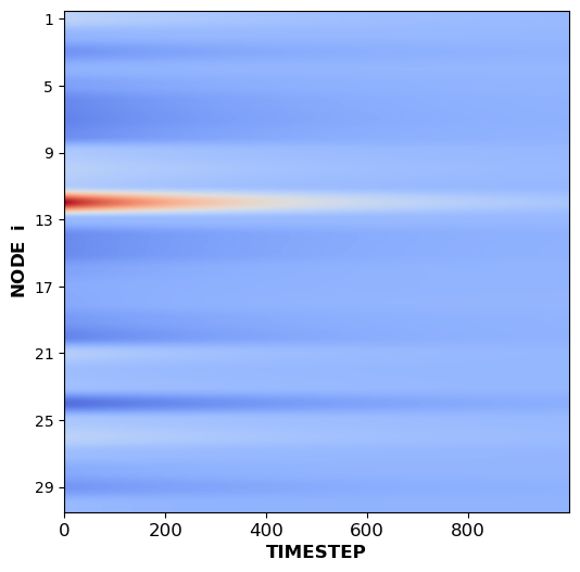
(a) Actual solution

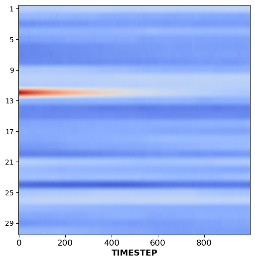
(b) Particle filter solution

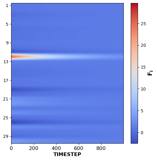
(c) Reduced order model solution

Figure 3:

5.2   Reaction-diffusion system on graphs

(a) ROM solution

(b) Actual solution

(c) Particle filter solution

Figure 4:

Figure 5: Comparing absolute value of errors of particle filter solution with ROM for the case of reaction-diffusion system, Equation (11). Here the black regions indicate grid points where the absolute value of error in the particle filter solution is less than ROM.

The results for the non-linear case are done for the alternating self-dynamics Brusselator model on a 40 node Erdős-R$\acute{e}$nyi random graph, also with the 4 point orthogonal method, number of trajectories is kept as two, number of particles taken in the particle filter step is 15000, T = 3, number of clusters p is kept as 30, $\epsilon_{1}=1e-5,\tau_{L}=0.1\,\mathrm{d}_{s}$, $\mathrm{d}_{s}$ represents the smallest degree of the given graph, $k=\mathrm{min(}{\lceil\frac{2n}{5}\rceil},50)$, $w_{k},\mu_{k}$ are assumed to be normally distributed with means as zero vector and variances $\zeta_{x}I,\zeta_{y}I$, where $\zeta_{x}=0.01,\zeta_{y}=1e-7$.

The graph obtained through the dynamic optimization step consisted of 286 sparse edges, with the given graph having 336 edges. The filtering step required a total of 50 updates were the prediction is done over a total of 100 timesteps.

6   Benchmarking the framework using neural ODEs

Neural ordinary differential equations (neural ODEs) have emerged as a robust framework for modelling and analyzing complex dynamical systems ([38], [39]). They provide a flexible approach to capturing the dynamics of a system by utilizing the principles of ordinary differential equations and neural networks. In traditional neural networks, the input is processed through a series of layers to produce an output. In neural ODEs, the dynamics of the system are modelled directly by specifying an ordinary differential equation. The differential equation represents how the hidden states evolve over time. The key idea behind neural ODEs is to learn the dynamics of the system by training the parameters of the differential equation using the adjoint sensitivity method ([33]); this allows the model to adapt and capture intricate temporal dependencies in the data. By leveraging the continuous-time nature of differential equations, neural ODEs offer several advantages, such as the ability to model irregularly sampled time-series data and handle variable-length inputs.

For demonstration let us consider the case of a linear dynamical system as shown below,

$$\frac{dx}{dt}=-Lx$$

Here $L$ is taken to be the Laplacian matrix of complete graph ${\mathbb{K}_{10}}$. $N=30$ observations are taken randomly from time $t=0$ to $t=0.05$. The neural network architecture is designed to have two hidden layers where the parameters are given by

$$\theta_{1}\in\mathbb{R}^{10\times 50},\theta_{2}\in\mathbb{R}^{50\times 50},\theta_{3}\in\mathbb{R}^{50\times 10},b_{1}\in\mathbb{R}^{50},b_{3}\in\mathbb{R}^{10}.$$

The neural network function is defined as

$$nn(x(t))=\sinh{(\theta_{3}\theta_{2}\theta_{1}x(t)+\theta_{3}\theta_{2}b_{1}+b_{3})}.$$ (11)

The cost function $J$ (Eq. 12) used to recover the parameters of the neural ODENet is mentioned below, we denote the parameter vector as $\theta$ consisting of $\theta_{1},\theta_{2},\theta_{3},b_{1}$ and $b_{3}$ after flattening,$\,\theta\in\mathbb{R}^{3560\times 1}.$

$$J(\theta)=\frac{1}{2}\sum_{k=1}^{N}||x_{k}-\tilde{x}_{k}||_{2}^{2}+\alpha_{1}\;||\theta||_{1}.$$ (12)

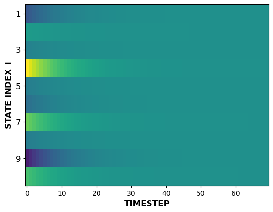
(a) Actual solution

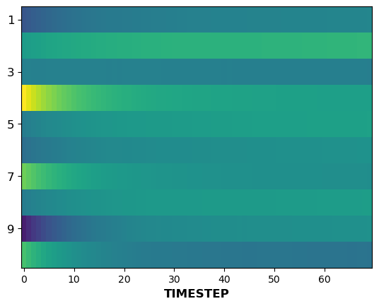
(b) Particle filter solution

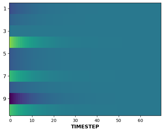
(c) ROM solution

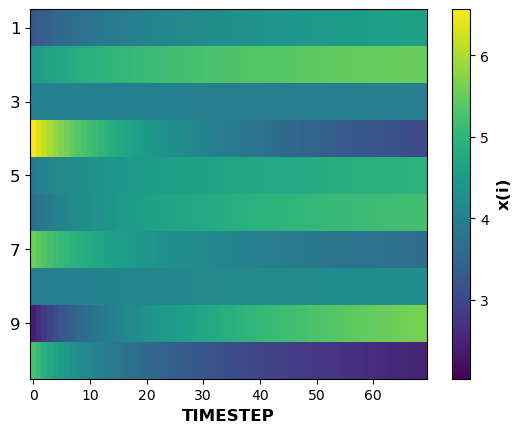
(d) neural ODE solution

Figure 6:

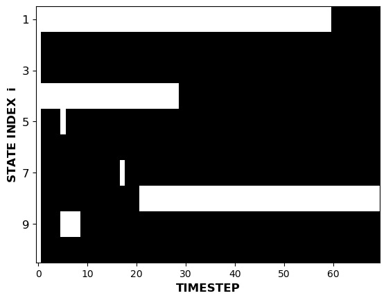
(a) Comparing absolute value of errors of particle filter with the neural ODE solution. Here the black regions indicate grid points where the absolute value of error in the particle filter solution is less than neural ODE solution.

(b) Comparing absolute value of errors of particle filter with the ROM solution. Here the black regions indicate grid points where the absolute value of error in the particle filter solution is less than ROM solution.

Figure 7:

The parameters are determined using the adjoint sensitivity method with the Euler discretization scheme. The number of clusters is kept at 40.

$$\bigg{\{}\begin{array}[]{l}x_{k+1}=x_{t}+\Delta t_{k}\;{nn(}x_{k})+A_{k+1}v_{k}+w_{k}\\ z_{k}=\rho\;\left(x_{k}-\bar{x}\right)+R_{k}\beta_{k}+\mu_{k\;}\end{array}$$

Updates at the $k$th iteration are made to vectors $\beta_{k}$ as the solution to the linear systems.

$$R_{k+1}\;\beta_{k} =z_{k+1}-\rho(x_{k+1}-\bar{x})$$

$A_{k+1},R_{k+1}$ are assigned as described in filtering step in Section 3.2, $x_{k+1}$ represents the solution at time-step $k+1$ determined as $x_{k+1}=x_{k}+\Delta t_{k}(nn(x_{k}))$ ($\Delta t_{k}=t_{k+1}-t_{k}$), the vector $v_{k}=\mathbf{0}_{n\times 1}$. The number of updates the experiment took is 41 where prediction is done for a total of 100 timesteps, number of particles in the particle filter step is kept as 20000, $w_{k},\mu_{k}$ are assumed to be normally distributed with means as zero vector and variances $\zeta_{x}I,\zeta_{y}I$, where $\zeta_{x}=0.01,\zeta_{y}=1e-3,\alpha_{1}=\frac{1}{3560}$.

7   Conclusion and discussion

The integration of key techniques from pattern recognition and stochastic filtering has shown promising potential in enhancing the outcomes achieved by the POD method. The effectiveness of this integration is demonstrated in Figure 3 for the linear case of diffusion and Figure 4 for the reaction-diffusion case with the chemical Brusselator model as reference. A basic neural ODENet framework was employed to establish a benchmark. The neural ODE solution exhibited significant deviation from the actual solution, as Figure 6(d) depicts. Nevertheless, when combined with projected measurements (Figure 6(c)), the particle filter solution (Figure 6(a)) provided reasonable approximations to the actual reaction-diffusion solution (Figure 6(a)). A comparative analysis of the absolute error between the particle filter and ROM methods, as illustrated in Figure 5, revealed that the particle Filter exhibited lower error rates across most grid points. Similar comparisons were made using the neural ODE framework (Figure 7). The graph, which is used for updating solutions in the filtering step, is sparse obtained from the dynamic optimization framework (Section 3.2), and the number of sparse edges obtained are given in (Section 5).

The complex systems which we consider are undirected, but complex systems involving directed graphs like the complex Ginzburg-Landau (CGL) equation as mentioned in [37] are not considered in this work, which will be the future scope of our work.

References

- [1] Dirk Brockmann and Dirk Helbing. The hidden geometry of complex, network-driven contagion phenomena. Science, 342(6164):1337–1342, 2013.
- [2] Sergei Maslov and I. Ispolatov. Propagation of large concentration changes in reversible protein-binding networks. Proceedings of the National Academy of Sciences, 104(34):13655–13660, 2007.
- [3] Muruhan Rathinam and Linda R. Petzold. A new look at proper orthogonal decomposition. SIAM Journal on Numerical Analysis, 41(5):1893–1925, 2003.
- [4] Redouane Lguensat, Pierre Tandeo, Pierre Ailliot, Manuel Pulido, and Ronan Fablet. The analog data assimilation. Monthly Weather Review, 145(10):4093–4107, 2017.
- [5] D.C. Park and Yan Zhu. Bilinear recurrent neural network. Proceedings of 1994 IEEE International Conference on Neural Networks (ICNN’94).
- [6] D.-C. Park. A time series data prediction scheme using bilinear recurrent neural network. In 2010 International Conference on Information Science and Applications, pages 1–7, Seoul, Korea (South), 2010. IEEE.
- [7] Julien Brajard, Alberto Carrassi, Marc Bocquet, and Laurent Bertino. Combining data assimilation and machine learning to emulate a dynamical model from sparse and noisy observations: A case study with the lorenz 96 model. Journal of Computational Science, 44:101171, 2020.
- [8] Peter D. Dueben and Peter Bauer. Challenges and design choices for global weather and climate models based on machine learning. Geoscientific Model Development, 11(10):3999–4009, 2018.
- [9] Ronan Fablet, Souhaib Ouala, and Cédric Herzet. Bilinear residual neural network for the identification and forecasting of geophysical dynamics. In 2018 26th European Signal Processing Conference (EUSIPCO), pages 1477–1481, Rome, 2018. IEEE.
- [10] Zichao Long, Yiping Lu, Xianzhong Ma, and Bin Dong. PDE-net: Learning PDEs from data. In Proceedings of the 35th International Conference on Machine Learning, page 9, 2018.
- [11] Marc Bocquet, Jérémie Brajard, Alberto Carrassi, and Laurent Bertino. Data assimilation as a learning tool to infer ordinary differential equation representations of dynamical models. Nonlinear Processes in Geophysics, 26(3):143–162, 2019.
- [12] Marc Bocquet, Jérémie Brajard, Alberto Carrassi, and Laurent Bertino. Bayesian inference of chaotic dynamics by merging data assimilation, machine learning and expectation-maximization. Foundations of Data Science, 2(1):55–80, 2020.
- [13] Pavel Sakov, Jean-Michel Haussaire, and Marc Bocquet. An iterative ensemble kalman filter in the presence of additive model error. Quarterly Journal of the Royal Meteorological Society, 144(713):1297–1309, 2018.
- [14] Alban Farchi, Patrick Laloyaux, Massimo Bonavita, and Marc Bocquet. Using machine learning to correct model error in data assimilation and forecast applications. Quarterly Journal of the Royal Meteorological Society, 147(739):3067–3084, jul 2021.
- [15] John D. Hedengren, Reza Asgharzadeh Shishavan, Kody M. Powell, and Thomas F. Edgar. Nonlinear modeling, estimation and predictive control in apmonitor. Computers & Chemical Engineering, 70:133–148, 2014. Manfred Morari Special Issue.
- [16] Lorenz T. Biegler. Nonlinear Programming. Society for Industrial and Applied Mathematics, 2010.
- [17] Chittaranjan Hens, Uzi Harush, Simi Haber, Reuven Cohen, and Baruch Barzel. Spatiotemporal signal propagation in complex networks. Nature Physics, 15(4):403–412, 2019.
- [18] Ming-Jun Lai, Jiaxin Xie, and Zhiqiang Xu. Graph sparsification by universal greedy algorithms, 2021. https://doi.org/10.48550/arXiv.2007.07161.
- [19] Daniel A. Spielman and Shang-Hua Teng. Spectral sparsification of graphs. SIAM Journal on Computing, 40(4):981–1025, 2011.
- [20] Daniel A. Spielman and Nikhil Srivastava. Graph sparsification by effective resistances, 2009.
- [21] Handbook of graph theory, combinatorial optimization, and algorithms. In Handbook of Graph Theory, Combinatorial Optimization, and Algorithms, pages 310–333. 2016.
- [22] Daniel A. Spielman and Shang-Hua Teng. Nearly-linear time algorithms for graph partitioning, graph sparsification, and solving linear systems. In Proceedings of the Thirty-Sixth Annual ACM Symposium on Theory of Computing, STOC ’04, page 81–90, New York, NY, USA, 2004. Association for Computing Machinery.
- [23] Stphane Boucheron, Gbor Lugosi, and Olivier Bousquet. Concentration inequalities. Stphane Boucheron, Gbor Lugosi, and Olivier Bousquet, 2013.
- [24] Miriam Farber and Ido Kaminer. Upper bound for the laplacian eigenvalues of a graph, 2011. https://doi.org/10.48550/arXiv.1106.0769.
- [25] Martin Grötschel, Sven Krumke, and Jörg Rambau. Online Optimization of Large Scale Systems. 01 2001.
- [26] R. Donald Bartusiak. Nlmpc: A platform for optimal control of feed- or product-flexible manufacturing. Assessment and Future Directions of Nonlinear Model Predictive Control, page 367–381.
- [27] Zoltan K. Nagy, Bernd Mahn, Rüdiger Franke, and Frank Allgöwer. Real-Time Implementation of Nonlinear Model Predictive Control of Batch Processes in an Industrial Framework, pages 465–472. Springer Berlin Heidelberg, Berlin, Heidelberg, 2007.
- [28] Abhishek Ajayakumar and Soumyendu Raha. Data assimilation for sparsification of reaction diffusion systems in a complex network, 2023. https://doi.org/10.48550/arXiv.2303.11943.
- [29] Jorge Nocedal and Stephen J. Wright. Numerical optimization. Springer, 2006.
- [30] David G. Luenberger and Yinyu Ye. Linear and nonlinear programming. Springer, 2021.
- [31] Fionn Murtagh and Pierre Legendre. Ward’s hierarchical agglomerative clustering method: Which algorithms implement ward’s criterion? Journal of Classification, 31(3):274–295, oct 2014.
- [32] Richard L. Burden, J. Douglas Faires, and Annette M. Burden. Numerical analysis. Cengage Learning, 2016.
- [33] John M. Lewis, Sivaramakrishnan Lakshmivarahan, and Sudarshan Kumar Dhall. Dynamic Data Assimilation: A least squares approach. Cambridge Univ. Press, 2009.
- [34] The MathWorks Inc. Matlab version: 9.13.0 (r2022b), 2022.
- [35] Tiancheng Li, Miodrag Bolic, and Petar M. Djuric. Resampling methods for particle filtering: Classification, implementation, and strategies. IEEE Signal Processing Magazine, 32(3):70–86, 2015.
- [36] Jeroen Elfring, Elena Torta, and Rob van de Molengraft. Particle filters: A hands-on tutorial. Sensors (Basel, Switzerland), 21(2):438, 2021.
- [37] Giulia Cencetti, Pau Clusella, and Duccio Fanelli. Pattern invariance for reaction-diffusion systems on complex networks. Scientific Reports, 8(1), 2018.
- [38] Wai Shing Fung and Nicholas J. A. Harvey. Graph sparsification by edge-connectivity and random spanning trees. CoRR, abs/1005.0265, 2010.
- [39] Hanshu Yan, Jiawei Du, Vincent Y. F. Tan, and Jiashi Feng. On robustness of neural ordinary differential equations, 2022.