Origin of Life Molecules in the Atmosphere After Big Impacts on the Early Earth
Abstract
The origin of life on Earth would benefit from a prebiotic atmosphere that produced nitriles, like HCN, which enable ribonucleotide synthesis. However, geochemical evidence suggests that Hadean air was relatively oxidizing with negligible photochemical production of prebiotic molecules. These paradoxes are resolved by iron-rich asteroid impacts that transiently reduced the entire atmosphere, allowing nitriles to form in subsequent photochemistry. Here, we investigate impact-generated reducing atmospheres using new time-dependent, coupled atmospheric chemistry and climate models, which account for gas-phase reactions and surface-catalysis. The resulting H2-, CH4- and NH3-rich atmospheres persist for millions of years, until hydrogen escapes to space. HCN and HCCCN production and rainout to the surface can reach molecules cm-2 s-1 in hazy atmospheres with a mole ratio of . Smaller ratios produce HCN rainout rates molecules cm-2 s-1, and negligible HCCCN. The minimum impactor mass that creates atmospheric is to kg (570 to 1330 km diameter), depending on how efficiently iron reacts with a steam atmosphere, the extent of atmospheric equilibration with an impact-induced melt pond, and the surface area of nickel that catalyzes CH4 production. Alternatively, if steam permeates and deeply oxidizes crust, impactors kg could be effective. Atmospheres with copious nitriles have K surface temperatures, perhaps posing a challenge for RNA longevity, although cloud albedo can produce cooler climates. Regardless, post-impact cyanide can be stockpiled and used in prebiotic schemes after hydrogen has escaped to space.
1 Introduction
Two essential aspects of life are a genome and catalytic reactions, so the presence of ribonucleotide molecular “fossils” in modern biochemistry (White, 1976; Goldman & Kacar, 2021) and the ability of RNAs to store genetic information and catalyze reactions have led to the hypothesis that RNA-based organisms originated early (Cech, 2012; Gilbert, 1986). This hypothesis proposes a stage of primitive life with RNA as a self-replicating genetic molecule that evolved by natural selection, which, at some point, became encapsulated in a cellular membrane and may have interacted with peptides from the beginning in the modified hypothesis of the RNA-Peptide World (e.g. Di Giulio, 1997; Muller et al., 2022). In any case, RNA must be produced abiotically on early Earth for such scenarios. Chemists have proposed several prebiotic schemes that require nitriles - hydrogen cyanide (HCN), cyanoacetylene (HCCCN), cyanamide (H2NCN), and cyanogen (NCCN) - to synthesize ribonucleobases, which are building blocks of RNA (Benner et al., 2020; Sutherland, 2016; Yadav et al., 2020).
Abiotic synthesis of nitriles in nature is known to occur efficiently from photochemistry in reducing N2-CH4 atmospheres (Zahnle, 1986; Tian et al., 2011). Indeed, Titan’s atmosphere, composed of mostly N2 and CH4, makes HCN, HCCCN and NCCN (Strobel et al., 2009).
Geochemical evidence does not favor a volcanic source for a CH4-rich prebiotic atmosphere. Redox proxies in old rocks indicate that Earth’s mantle was only somewhat more reducing 4 billion years ago (Aulbach & Stagno, 2016; Nicklas, 2019). Therefore, volcanoes would have mostly produced relatively oxidized gases like H2O, CO2 and N2 instead of highly reduced equivalents, H2, CH4 and NH3 (Holland, 1984; Catling & Kasting, 2017; Wogan et al., 2020). Thus, steady-state volcanism would have likely produced Hadean (4.56 - 4.0 Ga) air with CO2 and N2 as bulk constituents, whereas reducing gases, such as CH4, would have been minor or very minor.
However, Urey (1952) suggested that the prebiotic atmosphere was transiently reduced by large asteroid impacts. In more detail, Zahnle et al. (2020) argued that iron-rich impact ejecta could react with an impact-vaporized ocean to generate H2 (). As the H2O- and H2-rich atmosphere cools, their chemical equilibrium modeling with parameterized quenching finds that H2 can combine with atmospheric CO or CO2 to generate CH4. After several thousand years of cooling, the steam condenses to an ocean, leaving a H2 dominated atmosphere containing CH4. Zahnle et al. (2020) used a photochemical box model to show that such a reducing atmosphere would have generated prebiotic molecules like HCN. The reducing atmospheric state terminates when H2 escapes to space after millions of years.
Model simplicity in Zahnle et al. (2020) left critical questions unanswered. Their model of a cooling steam post-impact atmosphere did not explicitly simulate chemical kinetics pertinent to Earth, which may inaccurately estimate the generated CH4. Additionally, their photochemical box model did not include all relevant reactions or distinguish between different prebiotic nitriles (e.g. HCN and HCCCN). Finally, Zahnle et al. (2020) only crudely computed the climate of post-impact atmospheres, yet surface temperature is important for understanding the possible fate of prebiotic feedstock molecules. These molecules are needed to initiate prebiotic synthesis and must be available in the prebiotic environment.
Here, we improve upon the calculations made in Zahnle et al. (2020) using more sophisticated and accurate models of post-impact atmospheres. We estimate post-impact H2 production by considering reactions between the atmosphere and delivered iron, and equilibration between the atmosphere and impact-generated melt. Our model explicitly simulates the 0-D chemical kinetics of a cooling steam atmosphere, considering gas-phase reactions, as well as reactions occurring on nickel surfaces which catalyze CH4 production given that nickel is expected to be delivered by big impactors. After post-impact steam condenses to an ocean, we simulate the long-term evolution of a reducing atmosphere with a 1-D photochemical-climate model, quantifying HCN and HCCCN production and the climate in which they are deposited on Earth’s surface. Additionally, we discuss the possible fate and preservation of prebiotic molecules in ponds or lakes on Hadean land. Finally, we discuss how “lucky” primitive life was if created by post-impact molecules, given a need to not be subsequently annihilated by further impactors.
2 Methods
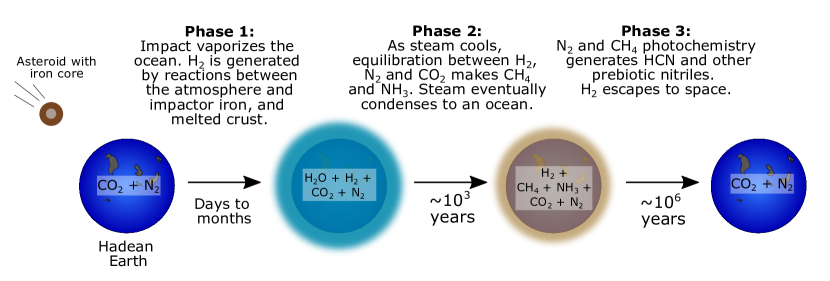
We organize our investigation of post-impact Hadean atmospheres in three phases of atmospheric evolution depicted in Figure 1. Below, we briefly describe our numerical models for each phase and complete descriptions can be found in the Appendix.
In Phase 1, an impactor collides with Earth, vaporizing the ocean, and H2 is generated by reactions between the atmosphere and iron-rich impact ejecta, and atmospheric reactions with an impact-produced melt pond. Our model of this phase (Appendix A) accounts for H2 generation from impactor iron by assuming each mole of iron delivered to the atmosphere removes one mole of oxygen. For example, Fe can sequester O atoms from steam:
| (1) |
Simulations that consider reactions between the atmosphere and impact-melted crust follow a similar procedure to the one described in Itcovitz et al. (2022). Our model requires that the atmosphere and melt have the same oxygen fugacity. The oxygen fugacity of the melt is governed by relative amounts of ferric and ferrous iron (Kress & Carmichael, 1991):
| (2) |
We assume that oxygen atoms can flow from the atmosphere into the melt (or visa-versa), and use an equilibrium constant for Reaction 2 from Kress & Carmichael (1991). Finally, we compute a chemical equilibrium state of the atmosphere (or atmosphere-melt system) at 1900 K using thermodynamic data from NIST for 96 gas-phase species (Appendix C.2). The result gives the estimated amount of H2 generated by an impact.
In Phase 2 of Figure 1, the steam atmosphere cools for thousands of years generating CH4 and NH3, and eventually, the steam condenses to an ocean. We simulate these events with the 0-D kinetics-climate box model fully described in Appendix B. The gas-phase model tracks 96 species connected by 605 reversible reactions (Appendix C.2), but we do not account for photolysis. The model also optionally accounts for reactions that occur on nickel surfaces using the chemical network described in Schmider et al. (2021). As discussed later in Section 3.2, nickel is potentially delivered to Earth’s surface by impacts which may catalyze methane production. In the model, atmospheric temperature changes as energy is radiated to space and is modulated by latent heat released from water condensation. We estimate the net energy radiated to space by using a parameterization of calculations performed with our radiative transfer code (Appendix D).
| Line absorption | Continuum CIA absorption | Rayleigh Scattering |
| H2O, CO2, CH4 | CO2-CO2, N2-N2, CH4-CH4, H2-CH4, H2-H2, H2O-H2O, H2O-N2 | N2, CO2, H2O, H2 |
During Phase 3, photochemistry generates HCN and other prebiotic molecules. Hydrogen in the H2 dominated atmosphere escapes to space over millions of years, ushering in the return of a CO2 and N2 atmosphere. We use our time-dependent photochemical-climate model, Photochem (Appendix C), to simulate this phase of atmospheric evolution. The model solves a system of partial differential equations approximating molecular transport in the vertical direction and the effect of chemical reactions, photolysis, condensation, rainout in droplets of water, and hydrogen atmospheric escape. Specifically, the model rains out haze particles and HCN among a few other atmospheric species listed in Appendix C.2. We simulate diffusion-limited and hydrodynamic hydrogen escape using Equation (47) in Zahnle et al. (2020). Our reaction network (Appendix C.2) acceptably reproduces the steady-state composition of Earth and Titan (Appendix Figure A9). When reproducing the chemistry of Earth and Titan we fix the temperature profile to measured values, rather than self-consistently compute the climate. We evolve the model equations accurately over time using the CVODE Backward Differential Formula (BDF) method (Hindmarsh et al., 2005). As the atmosphere evolves, we compute self-consistent temperature structures using the radiative transfer code described and validated in Appendix D. Unless otherwise noted in the text, our climate calculations use the opacities in Table 1, which is a subset of the opacities available in our radiative transfer code (Appendix Table A2). Climate calculations do not account for the radiative effects of clouds or hazes. However, our UV radiative transfer for computing photolysis rates do account for haze absorption and scattering.
3 Results
The following sections simulates the three post-impact phases of atmospheric evolution shown in Figure 1 for impactor masses between and kg (360 to 1680 km diameter) under various modeling assumptions.
3.1 Phase 1: Reducing the steam-generated atmosphere with impactor iron
Within days, a massive asteroid impact would leave the Hadean Earth with a global 2000 K rock and iron vapor atmosphere, the iron derived from the impactor’s core (Itcovitz et al., 2022). In the following months to years, energy radiated downward from the silicates would vaporize a large fraction of the ocean, adding steam to the atmosphere (Sleep et al., 1989). At this point, steam should rapidly react with iron to generate H2. Eventually, the iron vapor and then rock would rain out leaving behind a steam-dominated atmosphere containing H2, as well as CO2 and N2 from the pre-impact atmosphere. The sequence of metal followed by silicate condensation with falling temperature is loosely analogous to that of the well-known condensation sequence of the solar nebula.
Furthermore, the massive impact would generate a melt pool on Earth’s surface inside the impact crater, which may contain reducing impact-derived iron. The atmosphere and melt pool could react to a redox-equilibrium state. This could add or sequester H2 from the atmosphere, depending on whether the melt was more or less reducing than the atmosphere (Itcovitz et al., 2022).
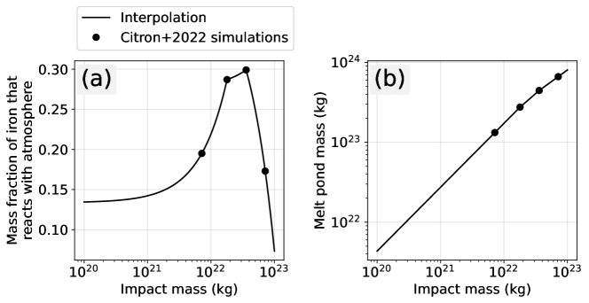
Recently, Itcovitz et al. (2022) used a smoothed-particle hydrodynamics (SPH) code with - particles of 150 - 250 km diameter to estimate the amount of H2 generated as these processes unfold under several different impact scenarios on the Hadean Earth. In their fiducial case (i.e. their “Model 1A”), they assume that 100% of iron delivered by an impactor is available to react and reduce a post-impact steam atmosphere. In another scenario, they assume that only 15 - 30% of impactor iron reacts with the steam atmosphere based on their SPH simulations (their “Model 1B”) (Citron & Stewart, 2022). For both cases, they also consider equilibration between the atmosphere and a melt pool (their “Model 2”, “Model 3A” and “Model 3B”). In their simulations, the melt pool is extremely reducing or more oxidizing depending on whether they assume it contains a fraction of the impactor’s iron, and they use SPH models to predict the amount of iron accreted to the melt pool (Citron & Stewart, 2022). Overall, they conclude that melt-atmosphere equilibration generates about as much H2 as their fiducial case as long as the iron delivered to the melt-atmosphere system can equilibrate. However, if iron delivered to the melt pool sinks into Earth and cannot react with the atmosphere, then approximately 2 - 10 times less H2 is produced compared to their fiducial scenario (see the erratum in Itcovitz et al. (2022)).
Itcovitz et al. (2022) considers impactors between and kg, and assumes the pre-impact Earth has 1.85 oceans of water, 100 bars CO2 and 2 bars of N2. However, we investigate impacts as small as kg, and our nominal model (Table 2) assumes only 0.5 bars of pre-impact CO2 motivated by models of the Hadean carbonate-silicate cycle (Kadoya et al., 2020) and assuming little mantle-hosted carbonate is vaporized. Therefore, we use a similar model (Appendix A) to the one described in Itcovitz et al. (2022) to predict the post-impact H2 for our alternative model assumptions (Table 2) and impactor sizes. Figure 2 shows the results.
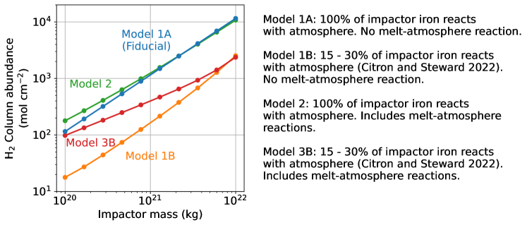
Our calculations give two end-member scenarios for impact H2 production which we consider for subsequent calculations in this article. The more optimistic case assumes that 100% of the impactor’s iron reacts with an atmosphere that is chemically isolated from a melt pool (“Model 1A” in Figure 2). Following Zahnle et al. (2020), we adopt this scenario as our nominal model throughout the main text. This assumption produces a similar amount of H2 as an atmosphere-melt system that retains most of the impactor’s iron (e.g. “Model 2” in Figure 2), which is consistent with Itcovitz et al. (2022). The “Model 2” calculation assumes the melt pool has an initial oxygen fugacity of FMQ-2.3 which is appropriate for a peridotite melt (Itcovitz et al., 2022).111FMQ is the fayalite-magnetite-quartz redox buffer. See Chapter 7 in Catling & Kasting (2017) for a discussion of redox buffers. However, our results are not sensitive to this assumption because, for “Model 2”, initial melt oxygen fugacities between FMQ and FMQ-4 changes the generated H2 by a factor of at most .
The less-optimistic case for H2 production is “Model 1B” in Figure 2, which assumes that only a fraction of the impactor iron reacts with an atmosphere ( to ), and that the latter does not react with a melt pool. We compute the fraction of available iron by extrapolating SPH simulations of impacts traveling at twice Earth’s escape velocity and colliding with Earth at a 45∘ angle (Appendix Figure A1), which is the most probable angle (Citron & Stewart, 2022). Most simulations shown in the main text have a complementary figure in the Appendix that makes this alternative pessimistic assumption regarding post-impact H2 generation.
| Parameter | symbol | value |
| Pre-impact ocean inventory | mol cm-2 (i.e. 1 ocean) | |
| Pre-impact CO2 inventory | 12.5 mol cm-2 (i.e. “0.5 bars”) | |
| Pre-impact N2 inventory | 36 mol cm-2 (i.e. “1 bar”) | |
| Impactor mass | - kg | |
| Iron mass fraction of the impactor | 0.33 | |
| Fraction of iron that reacts with atmosphere | 1.0 | |
| Impact angle | - | 45∘ |
| Impact velocity relative to Earth | - | km s-1 |
| Eddy diffusion coefficient | cm2 s-1 | |
| Aerosol particle radius | - | 0.1 m |
| Troposphere relative humidity | 1 | |
| Surface Albedo | 0.2 | |
| Temperature of the stratosphere | Tstrat | 200 K |
| Rainfall rate | molecules cm-2 s-1 (Modern Earth’s value) | |
| HCN deposition velocity | cm s-1 | |
| HCCCN deposition velocity | cm s-1 | |
| The source and inventory of surface H2O throughout the Hadean is debated (Miyazaki & Korenaga, 2022; Korenaga, 2021; Johnson & Wing, 2020) and even how much water is present on the modern Earth (e.g., Lécuyer et al. (1998) estimates 0.3-3 oceans in Earth’s mantle). Our nominal case of one modern ocean is one possibility among several. Based on Hadean carbon cycle modeling in Kadoya et al. (2020). Based on Figure 5 in Catling & Zahnle (2020). This is the “Model 1A” scenario for H2 production described near the end of Section 3.1 and in Figure 2. Assumed to be constant as a function of altitude. Estimated based on the HCN hydrolysis rate in the ocean (Appendix C.4). Assumed to the the same as HCN. | ||
3.2 Phase 2: The cooling post-impact steam atmosphere
After reactions between impact-derived iron and steam produce H2, the atmosphere would radiate at a rate determined by the optical properties of water vapor (Zahnle et al., 2020). Chemical reactions would initially be rapid, forcing the whole atmosphere to chemical equilibrium. Methane is thermodynamically preferred at lower temperatures (e.g., more methane is prefered in a gas at 1000 K than a gas at 1500 K), so it should become more abundant as the atmosphere cools. Eventually the atmosphere would reach a temperature where the reactions producing methane would be extremely sluggish compared to the rate of atmospheric cooling. At this point, the methane abundance would freeze, or quench. Ammonia would exhibit the same behavior as methane by initially rising in abundance then quenching when kinetics become slow. After several thousand years, water vapor condenses and rains out of the atmosphere to form an ocean.
We use the 0-D kinetics-climate box model described in Appendix B to simulate these events. By simulating each elementary chemical reaction, the model automatically computes methane and ammonia quenching as the atmosphere cools and temperature-dependent reactions slow. We first consider gas-phase kinetics, and later we will also consider nickel-surface kinetics.
Figure 3 shows our model applied to a kg ( km diameter) impactor. As the steam cools, ammonia quenches when the atmosphere is K, followed by CH4 quenching at K. After quenching, nearly half of the total carbon in the atmosphere exists as CH4. After 4200 years, the steam has largely rained out to form an ocean, leaving behind a H2-dominated atmosphere containing CH4 and NH3. NH3 is soluble in water, so a fraction should be removed from the atmosphere by dissolution in the newly formed ocean; however our simulations (e.g. Figure 3) do not account for this effect.
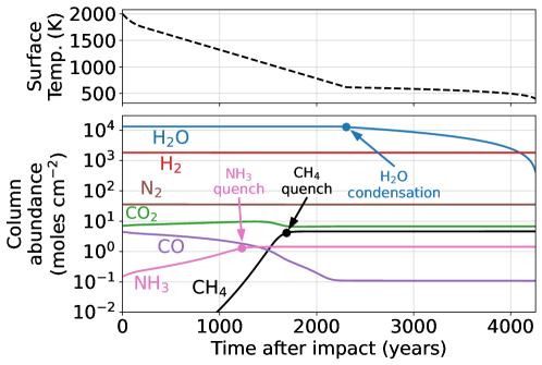
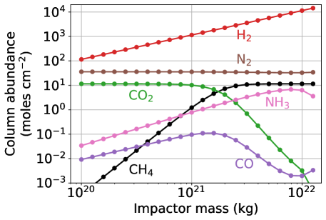
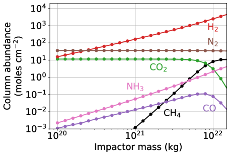
Figure 4 shows predicted atmospheric composition at the end of the steam atmosphere (e.g. at 4200 years in Figure 3) as a function of impactor mass. The calculations use gas-phase reactions, and our nominal model parameters (Table 2), including the assumption that 100% of the iron delivered by the impactor reacts with the steam atmosphere to make H2. For example, a kg impactor generates H2 moles cm-2 which would have a partial pressure of 1.2 bars if the atmosphere did not contain water vapor. A kg impactor generates H2 moles cm-2 which would have a “dry” partial pressure of 23.8 bars.222Partial pressures depend on the mean molecular weight of the atmosphere. The kg simulation in Figure 4 has 65.0 bars H2 before ocean vapor condenses, and would have 23.8 bars H2 if there was no water vapor in the atmosphere. Both scenarios have the same number of H2 molecules in the atmosphere, but have different partial pressures because of dissimilar mean molecular weights. To avoid ambiguity, we occasionally report partial pressures in “dry” bars, which is the partial pressure of a gas if the atmosphere had no water vapor. We find that most of the CO2 in the atmosphere is converted to CH4 for impactors larger than kg ( km diameter), and that bigger impacts generate more NH3, e.g., a kg impactor makes 0.013 “dry” bars of NH3. Reduced species like CH4 and NH3 are thermodynamically preferred in the thick H2 atmospheres generated by bigger impacts. Large impacts generate big amounts of hydrogen because they deliver more iron which more thoroughly reduces the atmosphere.
The Figure 4 calculations might underestimate the CH4 produced in the post-impact atmosphere because they ignore reactions occurring on nickel surfaces that can catalyze CH4 generation. If the impactors that struck the Earth during the Hadean resembled enstatite chondrite or carbonaceous chondrite composition then they would have contained 1% - 2% nickel (Lewis, 1992, Table 15). This nickel would have coexisted with the rock and iron vapor atmosphere that lasted months to years following a massive impact (Phase 1 in Figure 1). Metals along with silicates would have rained out as spherules covering the entire planet (Genda et al., 2017). As the impact-generated steam cooled, chemical reactions catalyzing CH4 production could have occurred on nickel surfaces in the bed of spherules (Schmider et al., 2021). These surface reactions could lower the quench temperature of CH4, causing more of the gas to be produced.
To estimate the effect of nickel catalysis on CH4 production, we use our kinetics-climate box model (Appendix B) with the nickel-surface reaction network developed by Schmider et al. (2021). The network is based on quantum chemistry calculations and about a dozen experiments from the literature. Our micro-kinetics approach is distinct from the empirical one taken by, e.g. Kress & McKay (2004), because our model tries to capture each elementary step of catalysis, rather than use a parameterization that is specific to certain experimental conditions.
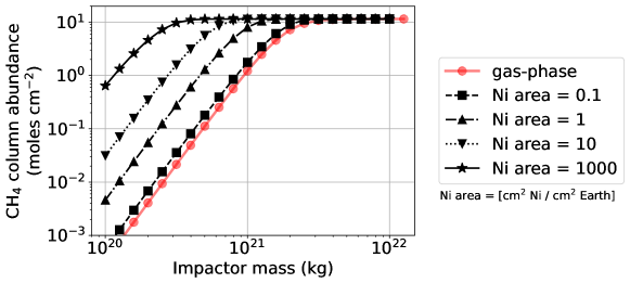
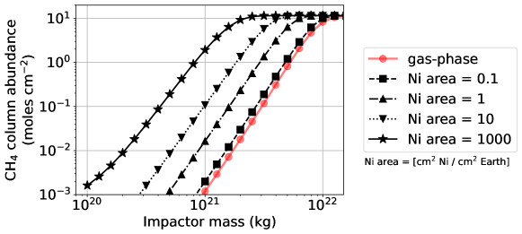
Figure 5 shows the quenched methane abundance as a function of impactor mass predicted by our model that includes nickel catalysts. The amount of CH4 generated depends strongly on the amount of available nickel surface area. Nickel areas bigger than 0.1 cm2 nickel / cm2 Earth permit more CH4 production compared to our gas-phase only model. Assuming a nickel area of 1000 cm2 nickel / cm2 Earth, then a Vesta-size impactor ( kg, 500 km diameter) could convert most CO2 in the pre-impact atmosphere to CH4.
Unfortunately, a precise nickel surface area is hard to estimate. The correct value depends on how the rock, iron and nickel spherules mix and precipitate to the surface, and furthermore, how effectively the atmosphere can diffuse through and react on exposed nickel. We do not attempt to compute these effects here, and instead estimate possible upper bounds. Consider a kg impactor (Vesta-sized) of enstatite chondrite composition, containing 2% by mass Ni (Lewis, 1992). If all this nickel is gathered into 1 mm spheres, a plausible droplet size according to Genda et al. (2017), then the total nickel surface area is cm2 nickel / cm2 Earth. An impactor ten times more massive would deliver ten times more nickel resulting in an upper bound Ni area that is one order of magnitude larger. Significantly smaller nickel particles are conceivable. There is experimental support for the formation of ultra-fine nm particles in the wake of impacts colliding with an ocean (Furukawa et al., 2007). For a Vesta-sized impactor, collecting all nickel into nm particles has a nickel area six orders of magnitude large than the 1 mm case - cm2 nickel / cm2 Earth. Overall, the larger nickel areas shown in Figure 5 may be within the realm of possibility. Alternatively, nickel might be buried by rock and iron when these materials condense out of the post-impact atmosphere, and that cm2 nickel / cm2 Earth is available for catalysis. In this case, gas-phase kinetics would determine the conversion of CO2 to CH4.
Figures 4 and 5 optimistically assume that all iron delivered by the impactor reacts with steam to make H2, however, this may not be the case (see Section 3.1). Therefore, in Appendix Figures A2 and A3 we recalculate Figures 4 and 5, but assume that only a fraction of the impactor’s iron reduces the steam atmosphere by extrapolating SPH simulations of impacts (“Model 1B” in Figure 2). The resulting H2, CH4, and NH3 production appear similar, except shifted by a factor of to larger impactors. The results are shifted by this amount because SPH simulations suggest approximately of impactor iron is delivered to the atmosphere, while the rest is either embedded in Earth, or ejected to space. We consider these supplementary calculations lower-bounds for impactor generated CH4 and NH3.
3.3 Phase 3: Long-term photochemical-climate evolution
Several thousand years after a massive impact, the steam-dominated atmosphere would condense to an ocean leaving behind a H2-dominated atmosphere containing CH4 and NH3 (e.g. at 4200 years in Figure 3). The reducing atmospheric state should persist for millions of years until hydrogen escapes (Zahnle et al., 2020).
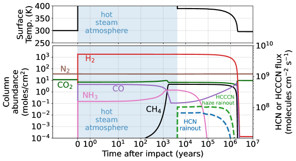
We simulate the long-term evolution of this hydrogen-rich atmosphere using a coupled one-dimensional photochemical-climate model (Appendix C). Figure 6 shows our model applied to the atmosphere following a kg ( km diameter) impactor. We assume a pre-impact atmosphere with 1 bar N2 and 0.5 bars of CO2, and simulate the cooling steam atmosphere with our kinetics-climate climate model (Section 3.2). Next, we use the end of the steam atmosphere simulation as initial conditions for our 1-D photochemical-climate model.
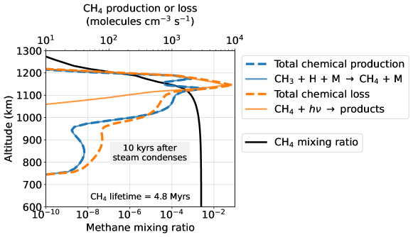
We find that N2 and CH4 photochemistry generates HCN in a hazy Titan-like atmosphere for about one million years until it is halted by hydrogen escape to space. In this model, the dominant channel producing HCN is where is ground (triplet) state of the methylene radical derived form methane photolysis. There are two other important paths. The first is followed by , and the second is and . In all pathways, hydrocarbon radicals (e.g., and ) are sourced from photolyzed CH4 and atomic N is derived from photolyzed N2, which both occur at high altitudes ( bar, Appendix Figure A5). The largest chemical loss of HCN is photolysis followed by . Other significant losses are paths that form HCCCN haze aerosols. HCN production and loss is our model is comparable to pathways discussed in similar studies (Zahnle, 1986; Tian et al., 2011; Rimmer & Rugheimer, 2019). We determined the chemical paths most important for producing and destroying HCN by studying column integrated reaction rates at 14,200 years in Figure 6.
In Figure 6, HCN mixes to the surface and rains out in droplets of water at a rate of molecules cm-2 s-1. HCN also dissolves into the ocean at a similar rate, where we assume it is eventually destroyed by hydrolysis (not shown in Figure 6). To emulate HCN dissolution and destruction in the ocean, we assume a cm s-1 deposition velocity justified in Appendix C.4. Additionally, a relatively small amount of HCN polymerizes to haze particles in our model via following Lavvas et al. (2008a), which falls and rains out in water droplets to the surface.
Our results differ from the simulations of Zahnle et al. (2020), which suggested that the duration of HCN production after an impact was limited by rapid photolysis of methane. The Figure 6 simulation finds that the CH4 lifetime is 4.8 million years because, following photolysis, CH4 efficiently recombines in a hydrogen rich atmosphere from the following reaction, which is well known in the atmospheres of the giant planets in out solar system (Appendix Figure A4).
| (3) |
Zahnle et al. (2020) did not account for Reaction 3. The lifetime of cyanide production is therefore instead determined by the timescale of hydrogen escape to space. Significant hydrogen escape permits the destruction of most atmospheric CH4 because Reaction 3 becomes inefficient, which in turn ceases CH4-driven HCN production.
In Figure 6, HCCCN is primarily destroyed by photolysis and produced by the following reaction from acetylene and the cyanide radical,
| (4) |
A fraction of produced HCCCN reacts to form aerosols via following Lavvas et al. (2008a). These polymers fall and mix toward the surface where they rainout in droplets of water at a rate of molecules cm-2 s-1. Most gas-phase HCCCN is either destroyed by photolysis or incorporated into aerosols, causing vanishingly small surface HCCCN gas pressures ( bar).
Our model approximates haze formation with the following three reactions: , , and . At 14,200 years in Figure 6, the first pathway dominates, forming g haze yr-1. At this same point in time the second and third pathways produce g yr-1 and g yr-1, respectively. The total haze production rate ( g yr-1) is comparable to values estimated by Trainer et al. (2006) for the early Earth based on laboratory experiments. Haze particles fall and rainout to the surface where they can hydrolyze and participate in prebiotic chemistry (Neish et al., 2010; Poch et al., 2012).
In Figure 6, impact-generated ammonia persists for nearly years. NH3 is primarily destroyed by photolysis, but then recombines from reactions with hydrogen:
| (5) | |||
| (6) |
Reactions 5 and 6 are relatively efficient in a hydrogen-rich atmosphere. Ammonia photolysis primarily occurs at the bar altitude, while haze is largely produced above the bar altitude. Therefore, haze particles partially shield ammonia from photolysis, extending the NH3 lifetime (Sagan & Chyba, 1997). Our model assumes the haze particles are perfect spheres with optical properties governed by Mie theory. Observations of Titan’s haze have revealed that hydrocarbon haze particles have a fractal structure which absorb and scatter UV more effectively than Mie spheres (Wolf & Toon, 2010). Therefore, our model likely overestimates NH3 photolysis in post-impact atmospheres.
Figure 6 assumes that all NH3 is in the atmosphere and that it does not rainout, but the gas is highly soluble in water and should dissolve in the ocean where it hydrolyzes to ammonium, NH. Later in Section 4.4.2, we show that for an atmosphere with 0.3 mol cm-2 NH3 and a 371 K ocean at , of NH3 would persist in the atmosphere, while the rest is dissolved in the ocean. For a hotter 505 K atmosphere with 6.8 mol cm-2 NH3, only 20% of ammonia dissolves in the ocean because solubility decreases with increasing temperature (Section 4.4.2). Ammonia dissolution in the ocean would protect it from photolysis perhaps lengthening the lifetime of ammonia in the atmosphere-ocean system. Overall, since our photochemical-climate model neglects NH3 ocean dissolution and likely overestimates NH3 photolysis, then we probably underestimate the lifetime of NH3 in Figure 6.
While HCN and HCCCN are produced in Figure 6, the surface temperature would be K primarily caused by H2-H2 collision-induced absorption (CIA), which has a significant greenhouse effect in thick H2 atmospheres like this one of 8.5 bars total pressure. The atmosphere cools to K after H2 escapes to space.
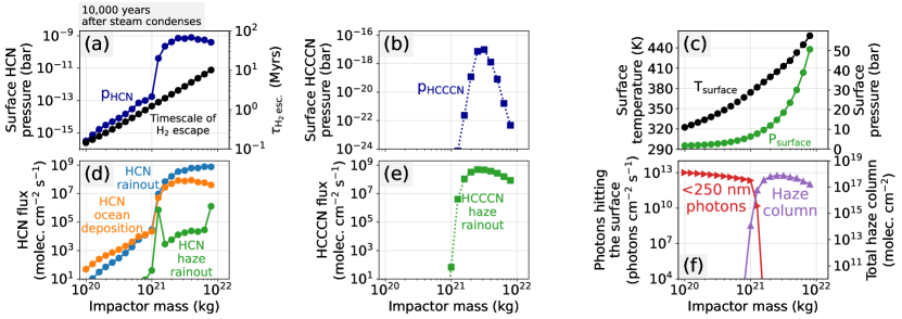
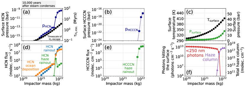
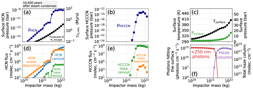
Figure 7 applies our model to various impactor masses. The results show the Hadean atmosphere 10,000 years after the post-impact generated steam atmosphere has condensed to an ocean. We choose 10,000 years after ocean condensation because this is adequate time for the atmosphere to reach a quasi-photochemical steady-state that does not change significantly until hydrogen escapes (e.g. Figure 6). Figure 7d and 7e show a sharp increase in the HCN and HCCCN production for impactors larger than kg ( km). Such large impacts generate (Figure 4), which makes a thick Titan-like haze (Trainer et al., 2006). Haze shielding causes CH4 photolysis to be higher in the atmosphere and closer to N2 photolysis, therefore the photolysis products of both species can more efficiently combine to make cyanides (Appendix Figure A5). Additionally, HCCCN production requires acetylene (Reaction 4), which is a haze precursor that accumulates when . These Titan-like atmospheres have bar surface HCN, and HCN ocean deposition and rainout rates between and HCN molecules cm-2 s-1 persisting on hydrogen escape timescales ( million years). HCCCN is incorporated into aerosols before raining out to the surface at a rate of up to HCCCN molecules cm-2 s-1.
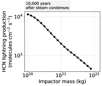
In addition to photochemistry, lightning should also generate HCN (Chameides & Walker, 1981; Stribling & Miller, 1987). Appendix Figure A8 shows HCN production from lighting for the same time period as the Figure 7 simulation using methods described in Chameides & Walker (1981). Assuming the same lightning dissipation rate as modern Earth’s, we find that lightning produces up to HCN molecules cm-2 s-1. This value is small compared to the - HCN molecules cm-2 s-1 produced from photochemistry after kg impacts.
Larger impacts generate a thicker H2 atmosphere which make the atmosphere warmer (Figure 7c). For impactors kg, which generate substantial HCN and HCCCN, the surface temperature is K. Figure 7f shows that impactors that produce substantial haze shield the surface from nm photons, which means that prebiotic schemes that require high energy UV light (e.g., Patel et al., 2015) would need to rely on stockpiling of the nitriles for later use.
The Hadean Earth CO2 concentration is uncertain. Models of the Hadean geologic carbon cycle argue for CO2 levels between and bar at 4 Ga with a median value of bar and a 95% uncertainty spanning to bar (Kadoya et al., 2020). However, these values might be unrealistically small because a large impact would warm surface rocks possibly causing carbonates to degass thereby increasing the atmospheric CO2 reservoir. Up to bars of CO2 may potentially be liberated from surface carbonates (Krissansen-Totton et al., 2021).
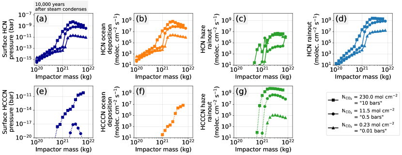
Figure 8 explores the effect of different pre-impact CO2 abundances on HCN and HCCCN production in post-impact atmospheres. The simulations are snapshots of the atmosphere 10,000 years after the impact-vaporized steam has condensed to an ocean. Larger pre-impact CO2 causes larger HCN and HCCCN production because it allows more CH4 to form in the cooling steam atmosphere. As discussed previously, CH4 is closely tied to photochemical cyanide generation. Regardless of the pre-impact CO2 concentrations, HCN and HCCCN production sharply increases for impactors larger than kg due to more efficient haze production (Figure 7, and corresponding text).
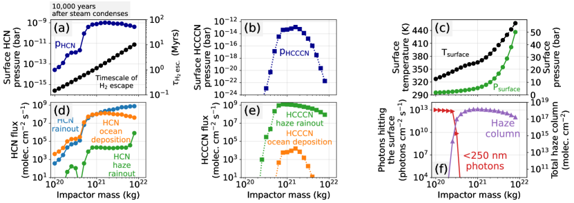
Figure 9 shows the state of the atmosphere after impacts of various size assuming 10 cm2 nickel / cm2 Earth is present in the steam atmosphere to catalyze methane production. The nickel causes more efficient conversion of CO2 to CH4 compared to the gas-phase only scenario (Figure 7) permitting greater production of HCN and HCCCN for smaller impactors. For example, a kg ( km) impactor which accounts for nickel catalysts (Figure 9) has comparable HCN and HCCCN production to a kg ( km diameter) impactor if no nickel catalysts are assumed in the cooling steam atmosphere (Figure 7).
A critical assumption in this section is that 100% of the iron delivered by impactors reacts with steam to generate H2. As discussed in Section 3.1, it is possible that the post-impact atmosphere is less thoroughly reduced by impactor iron. Appendix Figures A6 and A7 recalculate main text Figures 7 and 9, assuming that a fraction (approximately 15% to 30%) of impactor iron reduces the steam atmosphere based on SPH simulations (“Model 1B” in Figure 2). This alternative assumption requires that impactors times more massive are required to generate a haze-rich post-impact atmosphere with copious HCN and HCCCN production. For example, in Figure 7, recall that there is a sharp increase in cyanide production for impactors larger than kg ( km). Appendix Figure A6, which instead assumes a fraction of iron reduces the steam atmosphere, finds that the sharp increase in cyanide production occurs for impacts larger than kg ( km). However, the presence of nickel catalysts may permit large prebiotic nitrile production for smaller impactors, even under pessimistic post-impact H2 generation (Appendix Figure A7).
4 Discussion
4.1 Comparison to previous work
Recently, Zahnle et al. (2020) performed calculations of post-impact atmospheres using simpler models than the ones used in this article. Our results differ in several important ways. First, we find that our purely gas-phase model of the post-impact steam atmosphere (Section 3.2) predicts less CH4 generation than the model used in Zahnle et al. (2020). For example, Figure 4 predicts that most CO2 is converted to CH4 for impactors larger than kg. Figure 2 (top panel) in Zahnle et al. (2020), which is a comparable scenario, suggests a kg impactor is required to convert most of the atmospheric CO2 to CH4. The difference is likely caused by different approaches to computing CH4 quenching, or freeze-out, as the atmosphere cools. Our kinetics-climate model automatically computes CH4 quenching by tracking the elementary reactions producing and destroying CH4 along with many other atmospheric species. In most of our simulations of cooling post-impact atmospheres, CH4 quenches when the temperature is between and K. Zahnle et al. (2020) instead used equilibrium chemistry modeling with a parameterization for CH4 quenching derived from kinetics calculations of H2-dominated brown dwarf atmospheres (Zahnle & Marley, 2014). This parameterization predicts K CH4 quenching temperatures. The different quenching temperatures between our model and the Zahnle et al. (2020) model suggests that the Zahnle et al. (2020) kinetics parameterization is likely not suitable for a cooling steam-rich atmosphere.
The new photochemical model predicts longer post-impact CH4 lifetimes than the Zahnle et al. (2020) model. As mentioned previously, Zahnle et al. (2020) included CH4 photolysis, but neglected Reaction 3, which efficiently recombine photolysis products in hydrogen-rich atmospheres. In our model, these recombination reactions allow CH4 to persist in most post-impact atmospheres until hydrogen escapes to space ( millions of years). Zahnle et al. (2020) instead finds that CH4 is eradicated from the atmosphere before hydrogen escape.
Finally, nitrile production and rainout in our new model depend strongly on the presence of haze and the ratio, which was not the case in Zahnle et al. (2020). Our model finds that up to molecules cm-2 s-1 HCN and HCCCN is rained out in hazy post-impact atmospheres with (Figure 7). When , there is little haze, and HCN production is molecules cm-2 s-1 and HCCCN production is negligible. Haze causes CH4 and N2 photolysis products to be close in altitude so that they efficiently react to make cyanides (Appendix Figure A5). Additionally, HCCCN generation requires C2H2 in our model (Reaction 4), which is only abundant in hazy atmospheres. In contrast, Zahnle et al. (2020) finds that cyanide production rate in post-impact atmospheres is to molecules cm-2 s-1 regardless of the presence of haze and the ratio. Our results differ largely because our model is 1-D (has vertical transport), while the Zahnle et al. (2020) is a zero dimensional box model. HCN production depends on the proximity of CH4 and N2 photolysis, but a box model cannot account for this 1-D effect. Furthermore, Zahnle et al. (2020) does not distinguish between different prebiotic nitriles (e.g. HCN and HCCCN), or determine their surface concentrations and rainout rates. Also, Zahnle et al. (2020) does not have a coupled climate model.
Cometary and lightning sources of HCN are relatively small compared to our estimated photochemical production rates in haze-rich post-impact atmospheres. Todd & Öberg (2020) calculated that comets could deliver HCN molecules cm-2 s-1 to the Hadean Earth, a value orders of magnitude smaller than HCN from photochemistry in our most optimistic models. As discussed in Section 3.3, we find that HCN production from lightning in post-impact atmospheres to be at most HCN molecules cm-2 s-1 which is also small compared to UV photochemistry in a CH4 rich atmosphere. This result agrees with Pearce et al. (2022), who also finds that lightning-produced HCN is relatively insignificant.
Rimmer & Shorttle (2019) suggested that localized ultra-reducing magma rich in carbon and nitrogen might outgas HCN and HCCCN. They imagine this gas interacting with subsurface water causing high concentrations of dissolved prebiotic molecules, and therefore a setting for origin of life chemistry. While this idea may have merit, their calculations do not account for graphite saturation in magma, which may inhibit outgassing of reduced carbon-bearing species, like HCN (Hirschmann & Withers, 2008; Wogan et al., 2020; Thompson et al., 2022). Additionally, Rimmer & Shorttle (2019) did not self-consistently account for the solubility of gases in magma, which has been been hypothesized to prevent the outgassing of H-bearing gases, like CH4 or HCN (Wogan et al., 2020). Therefore, we argue that a hypothesized volcanic source of HCN and HCCCN requires further modeling and experiments before it can be compared to a photochemical source, but, in general, seems challenging.
Cerrillo (2022) recently used a climate model to predict the surface temperature of post-impact atmospheres with compositions predicted by Zahnle et al. (2020). They find surface temperatures K in some cases. However, the Cerrillo (2022) calculations do not include the effects of water vapor on the lapse rate in the troposphere. Latent heat from water condensation alters convection in the troposphere, greatly reducing the lapse rate when compared to a dry lapse rate. The result is a much cooler surface. Our climate calculations include the effects of water vapor on the lapse rate, which is why we predict surface temperatures K, even in the wake of a kg impact in Figure 7. All our climate simulations of post-impact atmospheres allow surface liquid water.
If a post-impact atmosphere of 2000 mol cm-2 H2 is all lost to space ( bar pure H2 atmosphere, or of the H2 in an ocean), that would shift D/H of the ocean heavier by 1.4% by hydrodynamic escape and Rayleigh fractionation (following Equation (16) in Zahnle et al. (2019) using an escape fractionation factor appropriate for an atmosphere where H2 dominates over CO2). This may be an underestimate of the D/H shift because the immediate post-impact oxidation of iron by steam probably produce H2 with a lower concentration of D than the steam that condense into an ocean. Experiments show isotopic fractionation in reaction of iron powder with steam at low temperatures (Smith & Posey, 1957), but we are unaware of high temperature experiments corresponding to post-impact conditions. In any case, cumulative big impacts during the Hadean that created highly reducing atmospheres would be expected to increase oceanic D/H additively, raising the ocean D/H from starting values that were ten (Piani et al., 2020) to tens of percent (Alexander et al., 2012) lighter than the modern ocean. Such an evolution with intermittent hydrogen escape in the Hadean is consistent both with D/H constraints and with the xenon isotope record (Avice et al., 2018), in which ionic xenon is dragged out to space by early hydrogen escape and the distribution of xenon isotopes becomes heavier (Zahnle et al., 2019).
4.2 Origin of life setting and stockpiling of cyanides
The Hadean Earth may have had less land but was likely speckled with hot-spot volcanic islands similar to modern-day Hawaii (Bada & Korenaga, 2018), and possibly had continental land (Korenaga, 2021) where nitriles could accumulate. The majority of HCCCN and HCN produced in post-impact atmospheres would dissolve or rainout into the ocean where it would be diluted and gradually removed by hydrolysis reactions (Miyakawa et al., 2002) or complexation with dissolved ferrous iron (Keefe & Miller, 1996). However, some of the nitriles would be deposited in lakes or ponds on land. We consider, first, equilibrium with atmospheric and, second, time-integrated deposition.
Nitrile concentrations in waterbodies on land in equilibrium with the atmosphere according to Henry’s law would be too small to participate in prebiotic schemes that form ribonucleotides. Our models predict HCN surface pressures up to bar (Figure 7). For a warm 373 K pond, Henry’s law predicts the dissolved HCN concentration is mol L-1. Yet, mol L-1 HCN is required for polymerization (Sanchez et al., 1967) and published prebiotic schemes can use 1 mol L-1 HCN (Patel et al., 2015).
Additionally, while nitriles are produced in post-impact atmospheres, waterbodies on land would likely be too warm for prebiotic chemistry. In the Figure 6 simulation, substantial HCN and HCCCN production occurs in the aftermath of big impacts when the surface temperature is K caused by a H2-H2 CIA greenhouse. Nickel catalysts permit big HCN and HCCCN production for surface temperatures as small as K (Figure 9). Nucleotide building blocks are fragile at such hot temperatures and conditions may not be conducive to an RNA world (Bada & Lazcano, 2002).
We propose that cyanides produced in hot post-impact atmospheres may instead be preserved, stockpiled, and concentrated, and used in prebiotic schemes at a later time when the climate is colder. Cyanide rainout and stockpiling could occur for millions of years until HCN production is halted by H2 escape to space (Figure 6). For example, if HCN rains out at molecules cm-2 s-1 over one million years (Figure 7), then g cm-2 HCN could be stockpiled assuming all molecules are preserved. Once H2 escapes, the surface temperature would drop to K (Figure 6), and over longer timescales the carbonate-silicate cycle might settle on even colder climates because impact ejecta promotes CO2 sequestration (Kadoya et al., 2020). In this cold climate, cyanide stockpiled into salts could be released as HCN or CN- into water bodies on land because of rehydration, volcanic or impact heating (Patel et al., 2015; Sasselov et al., 2020), or UV exposure (Todd et al., 2022). Liberation of cyanide could enable the prebiotic schemes that make RNA.
Toner & Catling (2019) investigated a mechanism for stockpiling cyanides. Their thermodynamic calculations show that HCN can be preserved as ferrocyanide salts in evaporating carbonate-rich lakes. However, the Toner & Catling (2019) numerical experiments were at 273 K and 298 K, which are far colder environments than the K surface temperatures that coincide with large HCN production in post-impact atmospheres (Figure 9). Although, Toner & Catling (2019) did not address stockpiling of HCCCN, cyanoacetylene can be captured by 4,5-dicyanoimidazole (DCI), a byproduct of adenine synthesis, to make crystals of 4,5-dicyanoimidazole (CV-DCI) (Ritson et al., 2022) and it is possible that other capture mechanisms are yet to be discovered. Overall, the feasibility of stockpiling prebiotic nitriles in post-impact conditions requires further geochemical modeling and experiments.
4.3 Impactor size and the likelihood of the origin of life
We hypothesize that might be an important threshold required for a post-impact atmosphere to produce useful concentrations of nitriles for origin of life chemistry. Figure 10 shows HCN and HCCCN haze rainout as a function of the atmospheric mole ratio for every post-impact simulation in this article. When , the atmosphere is hazy, and HCN and HCCCN are delivered to the surface at a rate of up to molecules cm-2 s-1. In contrast, atmospheres with rainout less than HCN molecules cm-2 s-1 and have surface HCN concentrations less than bar (Figure 7). Such small HCN concentrations may be challenging to stockpile as ferrocyanides (Toner & Catling, 2019). Additionally, modeled atmospheres with produce negligible HCCCN, yet the molecule is required in prebiotic schemes to synthesize pyrimidine (cytosine and uracil) nucleobase precursors to RNA (Powner et al., 2009; Okamura et al., 2019; Becker et al., 2019).
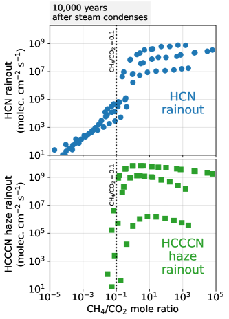
The impactor mass required to generate an atmosphere with is uncertain. Our optimistic model, which considers the effect of nickel-catalyzed methane production, requires a kg ( km) impactor (Figure 9). The lunar cratering record and abundance of highly siderophile elements Earth’s mantle imply that between 4 and 7 such impacts occurred during the Hadean (Marchi et al., 2014; Zahnle et al., 2020). Our least optimistic model needs a kg ( km) impact to create a post-impact atmosphere with because it assumes only a fraction of iron delivered to Earth reacts with the ocean to create atmospheric H2 (Appendix Figure A6). The Hadean only experienced 0 to 2 collisions this large (Zahnle et al., 2020). The precise minimum impactor mass to make an atmosphere with depends on the importance of atmospheric equilibration with a melt pond (Section 3.1, and Itcovitz et al. (2022)), the fraction of impactor iron that reduces the atmosphere, and the effect of Nickel and other surface catalysts on CH4 kinetics.
An additional consideration is that any progress toward the origin of life caused by an impact could be erased by a subsequent impact that sterilizes the planet. For example, suppose a km impact that vaporizes the ocean sterilizes the globe (Citron & Stewart, 2022). With our most pessimistic calculations for post-impact CH4 generation a km ( kg) impact is required to create an atmosphere that generates significant HCN and HCCCN. In this scenario, the last km impact favorable for prebiotic chemistry would likely be followed by a to km impact that would destroy any primitive life without rekindling it. Alternatively, our optimistic model for post-impact CH4 generation only requires a kg ( km) impact to create an atmosphere with . In this case, the final km impact that might kickstart the origin of life is unlikely to be followed by a slightly smaller km to km sterilizing impact.
A caveat to the reasoning in the previous paragraph is that ocean-vaporization may not have sterilized the planet because microbes could have possibly survived in the deep subsurface (Sleep et al., 1989; Grimm & Marchi, 2018).
In summary, we suggest that may be an important threshold for post-impact atmospheres to be conducive to the origin of life because they generate orders of magnitude larger surface HCN concentrations, and are the only modeled atmospheres capable of generating HCCCN. We find that the minimum impactor mass required to create a post-impact atmosphere with is between and kg ( to km). The value is uncertain because we do not know how effectively iron delivered by an impact reduces the atmosphere (Section 3.1), the importance of atmospheric equilibration with a melt pond (Section 3.1), and because it is hard to estimate a realistic surface area of nickel catalysts available during the cooling steam atmosphere (Section 3.2).
4.4 Model caveats and uncertainties
4.4.1 Hydrogen from crust-atmosphere reactions
Perhaps the most significant caveat to the modeling effort described above is that we did not consider H2 production from reactions between a hot post-impact atmosphere and solid, non-melted crust. Section 3.1 explores impact H2 made by two mechanisms: (1) reduction of the atmosphere by impact-derived iron and (2) atmospheric equilibration with a melt pond made by the impact. However, it is also conceivable that while the atmosphere is hot and steam-rich in the years following an impact (i.e. Phase 2), water vapor could permeate through and react with the solid crust to produce H2 by a process like serpentinization. Specifically, H2O reduction by FeO in the solid crust could make H2:
| (7) |
In our nominal model (Figure 4 and 7), we require a post-impact atmosphere has H2 mol cm-2 (i.e. the equivalent of converting 13% of Earth’s ocean to H2) in order to reach a and big nitrile production rates. Assuming a crustal FeO content of 8 wt% (Takahashi, 1986), then H2 mol cm-2 could be produced by reacting water with FeO in the top km of Earth’s lithosphere. The feasibility of extensive water-rock H2 generation depends on the permeability of the crust and the pressure gradients driving subsurface fluid circulation. For example, low permeability rocks with slow water circulation may not permit serpentinization of the upper crust within years while the atmosphere is hot and steam-rich. A comprehensive model is out of the scope of this article, but if attainable, significant water-rock reactions might produce a thick H2 atmosphere after relatively small impacts (e.g. kg) which favors a and significant nitrile generation.
Another possibility, which we do not investigate in detail, is that atmosphere-crust reactions occur in the immediate aftermath of a giant impact (i.e. Phase 1), rather than over as previously discussed. A large impact could produce a global ejecta blanket several kilometers thick of mixed hot water and rock. As water was vaporized to form a steam atmosphere, the water and rock slurry could chemically equilibrate, producing H2.
Zahnle et al. (2020) attempted to account for atmosphere-crust interaction by equilibrating the post-impact steam atmosphere (Phase 2) to a mineral redox buffer. For example, their Figure 5 assumes the atmosphere has a fixed oxygen fugacity set by the FMQ buffer at an assumed 650 K methane quench temperature. The calculation predicts most CO2 is converted to CH4 for impacts as small as kg, but Zahnle et al. (2020) did not determine whether such significant atmosphere-crust interaction is physically plausible.
4.4.2 Climate
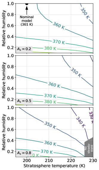
A shortcoming of this work is that our climate model is relatively simple. Throughout the Results section, our climate code assumes an isothermal 200 K stratosphere, a saturated adiabatic troposphere (i.e. relative humidity, ), and ignores clouds. However, many of our simulated post-impact atmospheres contain a hydrocarbon haze which should absorb sunlight and warm the stratosphere (Arney et al., 2016). Also, in a hydrogen-dominated atmosphere, water vapor has a larger molecular weight compared to the background gas which could inhibit convection (Leconte et al., 2017) and perhaps cause low relative humidities. Furthermore, low-altitude clouds reflect sunlight and should cool a planet while high clouds have a greenhouse warming effect (Goldblatt & Zahnle, 2011).
Figure 11 attempts to show the uncertainty in our climate calculations as a function of three free parameters: stratosphere temperature, relative humidity, and low-altitude clouds which we crudely approximate by varying the surface albedo. The calculation uses the composition of the atmosphere after a kg impact in Figure 9 immediately after the steam atmosphere has condensed to an ocean. Our nominal climate parameters ( K, , ) predict a 361 K surface temperature. A warm stratosphere caused by hydrocarbon UV absorption and high albedo low altitude clouds might cause the surface to be K colder than our nominal model, assuming water vapor is saturated. On the other hand, low relative humidities, which might be favored in convection-inhibited H2 dominated atmospheres, increase the troposphere lapse rate which warms the surface (Leconte et al., 2017). While Figure 11 gives a sense for the possible uncertainty in our climate calculations, it does not self-consistently simulate haze, relative humidity and clouds feedbacks. A more comprehensive model is required to resolve these nuances.
A further caveat is that our climate calculations ignore greenhouse warming from NH3 (Table 1). We choose to disregard the influence of NH3 because a substantial fraction of the gas should dissolve in the ocean (Zahnle et al., 2020), a process that our coupled photochemical-climate model cannot self-consistently account for. However, our climate model (Appendix D), when uncoupled to photochemistry, can partition gases between the atmosphere and ocean according to gas solubility and ocean chemistry. Below, we use this stand-alone climate model to determine the climate affects of NH3 in a post-impact atmosphere. NH3 should dissolve into an ocean by henry’s law, then hydrolyze to NH:
| (8) | |||
| (9) | |||
| (10) |
Therefore, the concentration of aqueous NH3 (in mol kg-1) is given by , where is the surface partial pressure of NH3 in bars and is the Henry’s law constant (mol kg-1 bar-1). Reactions 9 and 10 give the ammonium concentration to be , where and are equilibrium constants for each reaction. The Henry’s law constant for NH3 (in mol kg-1 bar-1) is (Linstrom & Mallard, 1998). The equilibrium constants for Reactions 9 and 10 are approximately and . We derived both of these parameterizations using the SUPCRT thermodynamic database (Johnson et al., 1992).
We implement this ocean chemistry into our stand-alone climate model (Appendix D), and compute the surface temperature after the kg impact in Figure 9 once the steam atmosphere has condensed to an ocean. The mol cm-2 of each gas are given in the Figure 11 caption. We use our nominal climate parameters ( K, , ), assume the total H2O reservoir is 1 modern ocean (15,000 mol cm-2) with pH = 7, and account for the radiative affects of NH3 in addition to the Table 1 opacities. The model predicts a 371 K surface temperature, which is 10 K warmer than calculations that do not include NH3 opacities or ocean dissolution. 96% of the ammonia reservoir is dissolved in the ocean.
Ammonia has a more substantial effect on climate after larger impactors. Consider the atmosphere after a kg impact in Figure 5 once steam has condensed to an ocean (0.008 mol cm-2 CO2, 11.5 mol cm-2 CH4, 32.6 mol cm-2 N2, 9122 mol cm-2 H2, 0.002 mol cm-2 CO, and 6.8 mol cm-2 NH3). Our climate model, which includes NH3 opacities and ocean dissolution, predicts a 505 K surface temperature with only 20% of the NH3 dissolved in the ocean because solubility decreases with increased temperature. This is 42 K hotter than our model that ignores NH3 greenhouse contributions (Figure 7). Overall, our climate calculations throughout most of this article perhaps underestimate the greenhouse warming by to K by ignoring NH3 opacities, but instead may overestimate surface temperature because do not account for the cooling effects of haze and low altitude clouds (Figure 11). Additional warming from NH3 would only be relevant for a fraction of the post-impact atmosphere, before ammonia is destroyed by photolysis (Figure 6).
4.4.3 Unknown chemical reactions and the effect of ions
While our chemical scheme for HCCCN successfully reproduces the HCCCN abundances in Titan’s atmosphere (Appendix Figure A9), it may lack many reactions relevant to post-impact atmospheres. Our sparse HCCCN network is necessary because currently few kinetic measurements are published in the literature.
Our photochemical model does not include ion chemistry, which is likely a reasonable simplification because ions are not important for HCN or HCCCN formation on Titan (Loison et al., 2015). Only some heavy hydrocarbons, like benzene (C6H6), rely on coupled neutral-ion chemistry to explain their observed abundances in Titan’s atmosphere (Hörst, 2017).
5 Conclusions
We use atmospheric models to investigate the production of prebiotic feedstock molecules in impact-generated reducing atmospheres on the Hadean Earth, updating simpler calculations made by Zahnle et al. (2020). We find that massive asteroid impacts can generate temporary H2-, CH4- and NH3-rich atmospheres, which photochemically generate HCN and HCCCN for the duration of hydrogen escape to space ( to years). The production of nitriles increases dramatically for haze-rich atmospheres that have mole ratios of . In these cases, HCN can rain out onto land surfaces at a rate of molecules cm-2 s-1, and HCCCN incorporated in haze rains out at a similar rate. Atmospheres with produce 3 to 4 orders of magnitude less HCN, and generate negligible HCCCN. The impactor mass required to create an atmosphere with is uncertain and depends on how efficiently atmosphere-iron, atmosphere-melt and atmosphere-crust reactions generate H2 and the surface area of nickel catalysts exposed to the cooling steam atmosphere. In an optimistic modeling scenario a kg ( km) impactor is sufficient, while in our least optimistic scenario a kg ( km) impactor is required.
We find that post-impact atmospheres that generate significant prebiotic molecules have K surface temperatures caused by a H2-H2 greenhouse which may be too hot for prebiotic chemistry, although the temperature may be cooler if reflective clouds occur. An alternative is that HCN and HCCCN generated in post-impact atmosphere are stockpiled. Cyanide can plausibly be stockpiled and concentrated in ferrocyanide salts and cyanoacetylene could be captured by byproducts of adenine synthesis into imidazole-based crystals (Ritson et al., 2022). HCN and HCCCN can be used to create nucleotide precursors to RNA millions of years after the impact, once the H2 has escaped to space, and the atmosphere has cooled to a more temperate state.
Nominally, the Hadean Earth appears to have experienced several impacts that would have produced an atmosphere that made significant prebiotic feedstock molecules. Like Earth, all rocky exoplanets accreted from impacts. Consequently, impact-induced reducing atmospheres may be a common planetary processes that provides windows of opportunity for the origin of exoplanet life.
Acknowledgements
We thank Joshua Krissansen-Totton for numerous conversations that have improved the atmospheric models used in this article. Conversations with Maggie Thompson, Sandra Bastelberger, and Shawn Domagal-Goldman also helped us create the Photochem and Clima models. We also thank Eric Wolf for advice on computing reliable k-distributions for climate modeling. Additionally, we thank Paul Mollière for conversations that helped us build Clima. Finally, we thank our two anonymous reviewers for constructive feedback that improved this article. N.F.W. and D.C.C. were supported by the Simon’s Collaboration on Origin of Life Grant 511570 (to D.C.C.). Also, N.F.W., D.C.C., and K.J.Z. were supported by NASA Astrobiology Program Grant 80NSSC18K0829 and benefited from participation in the NASA Nexus for Exoplanet Systems Science research coordination network. N.F.W. and D.C.C. also acknowledge support from Sloan Foundation Grant G-2021-14194. R.L. and K.J.Z. were supported by NASA Exobiology Grant 80NSSC18K1082. R.L. was additionally supported by NASA XRP 80NSSC22K0953.

Appendix A H2 generation from iron and molten crust
Here, we describe our model for atmospheric H2 generation in the days to months following a massive asteroid impact (Phase 1 in Figure 1). All our simulations assume a pre-impact atmosphere containing CO2, N2, and ocean water. First, we assume that half of the impactor’s kinetic energy heats the atmosphere and ocean water to K. We assume the atmosphere is heated to K because this is roughly the evaporation temperature of silicates. For our assumed impact velocity of km s-1, all impactor masses that we consider in the main text ( to kg) have kinetic energies joules delivering joules to the atmosphere which is larger than the joules required to vaporize an ocean (Sleep et al., 1989).
Next, our model assumes each mole of iron delivered reacts with the atmosphere and removes one mole of oxygen. The moles cm-2 of iron delivered to the atmosphere is
| (A1) |
Here, is the mass of the impact in grams, is the iron mass fraction of the impact, is the fraction of the impactor iron that reacts with the atmosphere, is the molar weight of iron, and is the area of Earth in cm2. Following Zahnle et al. (2020) we take . In main text, we assume (e.g. “Model 1A” in Figure 2), while the Appendix contains calculations with to based on extrapolations of the Citron & Stewart (2022) SPH impact simulations for impactors traveling at 20.7 km s-1 (e.g. “Model 1B” in Figure 2). To approximate equilibration between the delivered iron and the atmosphere, we simply remove of oxygen atoms from the atmosphere.
Our model also optionally considers reactions between the atmosphere and a melt pond generated by the impact. Our approach is similar to the one described in Itcovitz et al. (2022). We estimate the total mass of the melt pond () by interpolating SPH impact simulations from Citron & Stewart (2022) for a impact angle. The smallest impact they consider is kg, so we extrapolate their results down to kg. We additionally take the melted crust to be basaltic in composition except with variable initial amounts of ferric and ferrous iron. Effectively, this means that the initial oxygen fugacity of the melted crust is a free parameter because iron redox state is related to oxygen fugacity through the equilibrium reaction,
| (A2) |
We assume the oxygen atoms can flow from the atmosphere into the melt (or vice-versa) in order to bring Reaction A2 to an equilibrium state defined by Kress & Carmichael (1991) thermodynamic data. Our model also considers H2O gas dissolution in the melt using the Equation (19) solubility relation in Itcovitz et al. (2022).
Finally, given a heated post-impact atmosphere that has been reduced by impactor iron and, optionally, in contact with an melt pool, we compute thermodynamic equilibrium of the atmosphere-melt system at K. We choose 1900 K because any impact-produced silicate vapors should have condensed and rained out of the atmosphere, and the melt pool should have not yet solidified (Itcovitz et al., 2022). To find an equilibrium state, we first compute an equilibrium composition for the atmosphere alone using the equilibrium solver in the Cantera chemical engineering package (Goodwin et al., 2022) with our thermodynamic data (Appendix C.2). Next, to equilibrate the atmosphere-melt system, we perform a zero-dimensional kinetics integration for 1000 years at constant temperature and pressure with our reaction network (Appendix C.2). All reactions in our network are reversible thermodynamically, therefore integrating the kinetics forward in time should ultimately reach a state of thermodynamic equilibrium. Our integration includes additional reactions representing Reaction A2 and H2O dissolution in the melt. We arbitrarily choose forward reaction rates of s-1 for both reactions, then reverse the rates using the Kress & Carmichael (1991) equilibrium constant, and the Equation (19) solubility relation in Itcovitz et al. (2022). Overall, our approach finds a chemical equilibrium state between the atmosphere and the melt pond, and therefore an estimation of the amount of H2 generated from atmosphere-iron and atmosphere-melt reactions.
Our code for solving melt-atmosphere equilibrium is available at the following Zenodo link: https://doi.org/10.5281/zenodo.7802966.
Appendix B Kinetics model of a cooling steam atmosphere
We simulate the chemistry of a cooling post-impact atmosphere using a zero-dimensional kinetics-climate model. We assume the atmosphere’s composition, pressure, and temperature are homogeneous in all directions, and has a vertical extent of one atmospheric scale height (). For these assumptions, the following system of ordinary differential equations govern our model:
| (B1) |
| (B2) |
All variables and units are in Table A1. In Equation (B1), is the column abundance of species in mole cm-2, which changes because of gas-phase chemical reactions (production rate and loss rate ) and reactions occurring on surfaces ( and ). In Equation (B2), is surface temperature, which changes because of energy radiated to space (), and because of latent heat from H2O condensation (), where is the mass of H2O in the atmosphere. We approximate the energy radiated to space in ergs cm-2 s-1 from a steam-dominated atmosphere with the following parameterization:
| (B3) |
This parameterization fits calculations from our radiative transfer model (see Appendix D), which uses the a solar spectrum at 4.0 Ga derived from methods described in Claire et al. (2012).
We can rewrite Equation (B2), replacing using the ideal gas law and the definition of atmospheric scale height,
| (B4) |
Here, is the total atmospheric pressure in dynes cm-2, is gravitational acceleration in cm s-2, is the Boltzmann constant, is the mean molecular weight in g mol-1, and is Avogadro’s number. Therefore,
| (B5) |
Next, we must derive an expression for the steam condensation rate () in terms of known variables. Working in CGS units, the total pressure of the atmosphere is given by its gravitational force divided by Earth’s surface area ( cm2):
| (B6) |
Here, is the mass of the atmosphere in grams. We are considering steam-dominated atmospheres, therefore, the mass and pressure in the above relation is approximately equal to the mass of atmospheric H2O and the H2O partial pressure.
| (B7) | ||||
| (B8) |
Taking a time derivative of Equation (B8) yields
| (B9) |
We assume that the only processes changing the H2O mass in the atmosphere is condensation, which occurs in our model when steam becomes saturated. We further assume that the H2O partial pressure is fixed at saturation once steam condensation begins. We approximate the saturation vapor pressure of H2O, , using the Clausius-Clapeyron equation, assuming a temperature-independent latent heat, ,
| (B10) |
and are reference pressures and temperatures, respectively. Taking a time derivative of Equation (B10) yields
| (B12) |
Finally, we can substitute Equation (B12) into Equation (B5) and rearrange to solve for . The result below gives the rate of change of temperature when the steam is too hot to condense (), and when the steam is condensing ().
| (B13) |
Equations (B1) and (B13) are a system of ordinary differential equations, which we approximately solve over time using the CVODE BDF method developed by Sundials Computing (Hindmarsh et al., 2005). Additionally, for either gas-phase or surface reactions, we make use of the Cantera software library (Goodwin et al., 2022) to compute chemical production and destruction rates. Our code for solving the equations derived in this section is available at the following Zenodo link: https://doi.org/10.5281/zenodo.7802966.
| Variable | Definition | Units |
|---|---|---|
| Mixing ratio of species | dimensionless | |
| Number density of species | molecules cm-3 | |
| Total number density | molecules cm-3 | |
| Column abundance of species | mol cm-2 | |
| Total column abundance | mol cm-2 | |
| Density of the atmosphere | g cm-3 | |
| Specific heat capacity of the atmosphere | erg g-1 K-1 | |
| Net radiative energy leaving the atmosphere | erg cm-2 s-1 | |
| Altitude | cm | |
| Time | seconds | |
| Total chemical production of species | molecules cm-3 s-1 | |
| Total chemical loss of species | molecules cm-3 s-1 | |
| Total chemical production of species from surface reactions | molecules cm-2 s-1 | |
| Total chemical loss of species from surface reactions | molecules cm-2 s-1 | |
| Production and loss of species from rainout | molecules cm-3 s-1 | |
| Production and loss of species from condensation and evaporation | molecules cm-3 s-1 | |
| Vertical flux of species | molecules cm-2 s-1 | |
| Eddy diffusion coefficient | cm-2 s-1 | |
| Molecular diffusion coefficient | cm-2 s-1 | |
| , The scale heights of species | cm | |
| , The average scale height. | cm | |
| Avogadro’s number | molecules mol-1 | |
| Boltzmann’s constant | erg K-1 | |
| Gas constant | erg mol-1 K-1 | |
| Molar mass. is mean molar mass of the atmosphere, and is the molar mass of species | g mol-1 | |
| Catalyst surface area per atmospheric column | cm2 catalyst / cm2 Earth | |
| Latent heat of H2O condensation | erg g-1 | |
| Area of Earth’s surface | cm2 | |
| Relative humidity | dimensionless | |
| Optical surface albedo | dimensionless | |
| Atmospheric pressure. is the partial pressure of species . | dynes cm-2 | |
| Mass of the atmosphere. is the mass of species . is the mass of an impactor. | g | |
| Gravitational acceleration | cm s-2 | |
| Thermal diffusion coefficient of species . We neglect this term () | dimensionless | |
| Fall velocity of a particle | cm s-1 | |
| Temperature. is the surface temperature. | K |
Appendix C The Photochem model
To simulate the photochemistry of post-impact reducing atmospheres, we developed a photochemical model called Photochem. The model is a re-written and vastly updated version of PhotochemPy (Wogan et al., 2022). Photochem is written in modern Fortran and C, with a Python interface made possible by Cython (Behnel et al., 2010). This article uses Photochem version v0.3.14 archived in the following Zenodo repository: https://doi.org/10.5281/zenodo.7802921.
The following sections briefly describe the fundamental model equations solved by Photochem, our chemical network, and validates the model against observations of Earth and Titan.
C.1 Model equations
We begin our derivation of the equations governing Photochem with modified versions of Equations B.1, B.2 and B.29 in Catling & Kasting (2017):
| (C1) | |||
| (C2) | |||
| (C3) |
Table A1 explains the variables and their units. Equation (C1) states that molecule concentration ( in molecules cm-3) changes over time at a point in space because of vertical movement of particles (), and chemical reactions, rainout or condensation/evaporation (, , , and ). The equation is 1-D, because it only considers vertical gas transport and differs from Equation B.1 in Catling & Kasting (2017) because we explicitly include rainout and condensation. Equation (C2) states that the flux of gases () is determined by eddy and molecular diffusion, and Equation (C3) assumes that the flux of particles () is given by eddy diffusion and the rate particles fall through the atmosphere.
Many 1-D photochemical models further simplify Equation (C1) by assuming that total number density does not change over time (). Using this assumption, Equation (C1) is recast in terms of evolving mixing ratios () rather than number densities (see Appendix B.1 in Catling & Kasting (2017) for a derivation). Such models assume a time-constant temperature profile. The surface pressure is also prescribed, and pressures above the surface are computed with the hydrostatic equation. In order to guarantee that all mixing ratios in the atmosphere sum to 1, models assume a background filler gas with a mixing ratio . N2, CO2 or H2 are common choices for the background gas, depending on the atmosphere under investigation. By definition, the background gas is not conserved. This approach is valid for steady-state photochemical calculations, and is also reasonable for atmospheric transitions which maintain approximately constant surface pressure and atmospheric temperature. The Photochem code contains an implementation of this traditional approach to photochemical modeling.
Unfortunately, solving a simplified version of Equation (C1) in terms of mixing ratios does not work well for post-impact atmospheric modeling. For example, a post-impact atmosphere can contain 10 bars of H2 which escapes to space over millions of years, lowering the surface pressure to a 1 bar N2 dominated atmosphere (e.g. Figure 6). Traditional photochemical models fail to simulate this scenario because it is not reasonable to assume a single background gas and time-constant surface pressure. Additionally, most models fix atmospheric temperature during any single model integration, but surface temperature should change significantly as impact-generated H2 escapes to space.
Therefore, Photochem implements a code that solves Equation (C1) in terms of number densities () without the assumption of fixed surface pressure or a background gas. This approach requires slight modifications to Equation (C2) and (C3) which we describe below. Consider the hydrostatic equation and ideal gas law
| (C4) | |||
| (C5) |
Substituting the ideal gas law in the hydrostatic equation yields
| (C6) | |||
| (C7) |
After rearrangement and substituting the definition of scale height,
| (C8) |
Now consider the following expansion using the quotient rule
| (C10) |
Finally, we can substitute Equation (C10) into Equations (C2) and (C3) to derive new equations for the flux of gases and particles
| (C11) | |||
| (C12) |
We then apply a finite-volume approximation to the Equation (C1) system of particle differential equations using fluxes for gases and particles given by Equations (C11) and (C12), which results in a system of ordinary differential equations. We use a second-order centered scheme for all spatial derivatives except falling particles, which use a first-order upwind scheme for stability. Photochem evolves the finite volume approximate forward in time using the CVODE BDF method developed by Sundials Computing (Hindmarsh et al., 2005). The model assumes no background gas, and surface pressure can evolve over time as, for example, gases escape to space. Additionally, our model computes a self-consistent temperature structure within each time step using the Clima radiative transfer code (Appendix D) assuming a pseudo-moist adiabatic troposphere connected to an isothermal upper atmosphere.
An additional challenge of post-impact atmospheres is that the scale height changes by a factor of or more when H2 escapes leaving behind a N2 or CO2 dominated atmosphere (Figure 6). Most relevant photochemistry occurs at pressures bar, and so we choose a model domain which starts at the surface and extends to an altitude that is approximately this pressure. However, suppose we choose a model domain extending to km (i.e. the bar level) appropriate for an H2 dominated atmosphere. After H2 escapes to space, all relevant photochemistry would occur below km, in the bottom several grid cells of the model. Therefore, the important photochemistry would be poorly resolved and inaccurate, and the extremely small pressures at the top of the model domain would likely cause numerical instability. Our solution is to adaptively adjust the model domain so it is always appropriate for atmospheres scale height. We use the root finding functionally in CVODE BDF to halt integration whenever the pressure at the top of the atmosphere falls below bar and lower the top of the model domain before continuing integration. This procedure is done automatically tens to hundreds of times during each post-impact integration.
C.2 Chemical network, photolysis cross sections and thermodynamic data
Our chemical reactions, photolysis cross sections, and thermodynamic data used for all gas-phase kinetics are archived in the following Zenodo repository: https://doi.org/10.5281/zenodo.7802962. Chemical reactions and thermodynamic data are in the file “reaction_mechanisms/zahnle_earth.yaml”, and photolysis cross sections are in the folder “xsections/”. All thermodynamic data is from the NIST Chemistry WebBook (Linstrom & Mallard, 1998). The chemical and photolysis reactions are an updated version of rates presented in Zahnle et al. (2016).
In this article, our model simulates rainout in droplets of water for the following species: particles, OH, CN, HCN, C2H4, NO, HO2, N2O, H2O2, O3, NO2, NO3, HNO2, HNO3, C2H6, CH3OH, CH3CHO, C3H6, CH3CN.
C.3 Model validation
Figure A9 shows Photochem applied to Earth and Titan compared to observations gathered from the literature. All boundary conditions and settings for each model are archived in the “ModernEarth” and “Titan” templates in the following Zenodo repository: https://doi.org/10.5281/zenodo.7802921. Our model of Titan fixes the surface CH4 mixing ratio to volume mixing ratio, permits H2 escape at the diffusion-limited rate, and allows aerosols to fall to Titan’s surface, but otherwise has zero-flux boundary conditions. We ignore the effects of galactic cosmic rays, which causes our model to under-predict the nitrile haze production in the lower atmosphere (Lavvas et al., 2008b). Additionally, we neglect ion chemistry which is argued to be important for the formation of large hydrocarbons (e.g., ), but inconsequential for smaller molecular weight species. Despite these omissions, Photochem broadly reproduces the main cyanide chemistry on Titan.
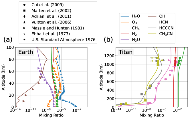
C.4 Deposition velocity of HCN
Our photochemical-climate simulations of post-impact atmosphere assume a HCN surface deposition velocity of cm s-1. Here, we describe a simple model of HCN hydrolysis in the ocean which justifies this value.
Motivated by Appendix 3 in Kharecha et al. (2005), we imagine a two-box ocean model with a surface ocean of depth m and a deep ocean ( km). We assume HCN transport into the ocean is governed by a stagnant boundary layer model (see Figure 3 in Kharecha et al. (2005)), where it is destroyed by hydrolysis reactions. HCN is mixed between the surface and deep ocean reservoirs by a turnover velocity, , which we nominally take to be cm s-1 which is appropriate for modern Earth. Under these circumstances, the following system of ordinary differential equations governs the concentration of HCN in the surface and deep ocean.
| (C13) | |||
| (C14) |
Here, and are the concentration of HCN in the surface and deep ocean, respectively, in mol L-1, is a constant equal to molecules mol-1 L cm-3, is the depth of the surface ocean, and is the depth of the deep ocean. We compute the temperature and pH dependent hydrolysis rate coefficient, , following Miyakawa et al. (2002). is the HCN flux into the ocean in molecules cm-2 s-1, which is determined by a stagnant boundary layer model:
| (C15) |
We assume the piston velocity of HCN is cm s-1, which is the same as the piston velocity of CO (Kharecha et al., 2005, Table 1). Also, is the henry’s law coefficient for HCN. The flux of a gas can also be parameterized with a deposition velocity ():
| (C16) | ||||
| (C17) |
Here, we assume that the temperature and pH of the ocean is uniform, and that the temperature of the surface air is the same as the temperature of the ocean.
Figure A10 computes the deposition velocity of HCN using Equation (C17) over a wide range of ocean temperatures and pH. Kadoya et al. (2020) used a model of the geologic carbon cycle to argue that the Hadean ocean was moderately alkaline (pH ). Therefore, we choose a HCN deposition velocity of cm s-1 for our nominal model because it a reasonable approximation of the pH case over a wide range of temperatures. Additionally, we assume that HCCCN has the same deposition velocity as HCN, also caused by hydrolysis reactions in the ocean.
We have re-run our photochemical-climate simulations of post-impact atmospheres with order-of-magnitude larger and smaller HCN deposition velocities. The results are qualitatively unchanged. For example, assuming cm s-1 for a kg impactor in Figure 7 causes one order of magnitude smaller HCN ocean deposition. However, the HCN rainout and HCN surface pressure is unchanged because HCN rainout dominates over the HCN ocean deposition.
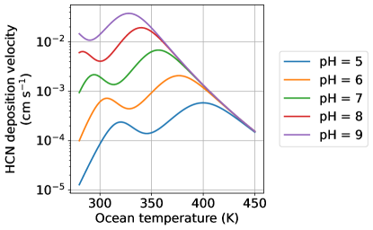
Appendix D The Clima radiative transfer and climate model
To simulate the climate of post-impact atmospheres, we developed a new radiative transfer and climate code called Clima. We approximately solve the radiative transfer equation using standard two-stream methods (Toon et al., 1989). The code includes opacities representing photolysis, Rayleigh scattering, collision-induced absorption, and approximates line absorption with k-distributions. All available opacities and citations, except photolysis cross sections, are listed in Table A2. In this article, to account for line absorption of multiple species, we use the “random overlap with resorting and rebinning” method described in Amundsen et al. (2017).
Figure A11 shows a thermal emission spectra computed with Clima for a two bar pure CO2 atmosphere on Mars with a 250 K surface temperature. This same benchmark has been computed by several other radiative transfer codes: SOCRATES (Wolf et al., 2022, Figure 2), ExoRT (Wolf et al., 2022, Figure 2), SMART (Figure A11), and the radiative transfer code used in Kopparapu et al. (2013) (their Figure 1). All codes estimate the total outgoing thermal energy to be between 86 and 94 W m-2, which is comparable to the value computed by Clima (92.9 W m-2).
The Clima code also includes an adiabatic climate model which we use in Section 4.4.2. Given partial pressures of gases at the surface, the code draws a pseudo-adiabat temperature profile upward using Equation (1) in Graham et al. (2021) until the temperature reaches an assume isothermal stratosphere. The code is general and can consider any number of condensing species, but H2O is the only relevant condensible for post-impact atmospheres. Finally, to find an equilibrium climate, we solve a nonlinear equation for the surface temperature that balances incoming solar and outgoing longwave radiation. Each iteration of the nonlinear solve involves drawing an adiabat upward then computing the solar and infrared radiative fluxes.
We have validated the stand-alone climate model in Clima by reproducing the calculations in Wordsworth et al. (2017) of early Mars with CO2 and H2 atmospheres (left panel of Figure 2 in Wordsworth et al. (2017)). Furthermore, we predict the runaway greenhouse limit to be 291 W m-2, which is in acceptable agreement with the literature (e.g., Kopparapu et al., 2013). Finally, we have also confirmed that our code for drawing pseudo-moist adiabats reproduces the code used in Graham et al. (2021).
The version of Clima used in this article (v0.3.7) is archived on Zenodo (https://doi.org/10.5281/zenodo.8060772), while the most up-to-date version can be found on GitHub (https://github.com/Nicholaswogan/clima).
| Opacity type | Opacity | Notes | Citation |
| k-distributions | H2O | HITEMP2010 for 0 to 30,000 cm-1 and HITRAN2016 for 30,000 to 42,000 -1. Voigt line shape with 25 cm-1 cutoff. Assumes Earth air broadening coefficients. Plinth or base is removed because this opacity is combined with MT_CKD H2O continuum. | Rothman et al. (2010); Gordon et al. (2017) |
| CO2 | HITEMP2010. Sub-Lorentzian line shape with 500 cm-1 cutoff. Assumes self-broadening coefficients. | Rothman et al. (2010) | |
| CH4 | HITEMP2020. Voigt line shape with 25 cm-1 cutoff. Assumes Earth air broadening coefficients. | Hargreaves et al. (2020) | |
| CO | HITEMP2019. Voigt line shape with 25 cm-1 cutoff. Assumes self-broadening coefficients. | Li et al. (2015) | |
| O2 | HITRAN2016. Voigt line shape with 25 cm-1 cutoff. Assumes Earth air broadening coefficients. | Gordon et al. (2017) | |
| O3 | HITRAN2016. Voigt line shape with 25 cm-1 cutoff. Assumes Earth air broadening coefficients. | Gordon et al. (2017) | |
| NH3 | HITRAN2016. Voigt line shape with 25 cm-1 cutoff. Assumes Earth air broadening coefficients. | Gordon et al. (2017) | |
| CIA | H2-H2 | - | Mollière et al. (2019) |
| H2-He | - | Mollière et al. (2019) | |
| N2-N2 | - | Mollière et al. (2019) | |
| CH4-CH4 | - | Karman et al. (2019) | |
| N2-O2 | - | Karman et al. (2019) | |
| O2-O2 | - | Karman et al. (2019) | |
| H2-CH4 | - | Karman et al. (2019) | |
| CO2-CO2 | - | Karman et al. (2019) | |
| CO2-CH4 | - | Karman et al. (2019) | |
| CO2-N2 | - | Karman et al. (2019) | |
| N2-H2 | - | Karman et al. (2019) | |
| Rayleigh scattering | N2 | - | Keady & Kilcrease (2002); Penndorf (1957) |
| CO2 | - | Keady & Kilcrease (2002); Shemansky (1972) | |
| O2 | - | Keady & Kilcrease (2002); Penndorf (1957) | |
| H2O | - | Keady & Kilcrease (2002); Ranjan & Sasselov (2017); Murphy (1977) | |
| H2 | - | Keady & Kilcrease (2002) | |
| All k-distributions are computed using HELIOS-K (Grimm et al., 2021). Rayleigh scattering opacities are computed using a parameterization from Vardavas & Carver (1984). | |||
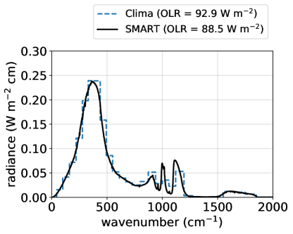
References
- Adriani et al. (2011) Adriani, A., Dinelli, B., Lopez-Puertas, M., et al. 2011, Icarus, 214, 584
- Alexander et al. (2012) Alexander, C. O., Bowden, R., Fogel, M., et al. 2012, Science, 337, 721
- Amundsen et al. (2017) Amundsen, D. S., Tremblin, P., Manners, J., Baraffe, I., & Mayne, N. J. 2017, Astronomy & Astrophysics, 598, A97
- Arney et al. (2016) Arney, G., Domagal-Goldman, S. D., Meadows, V. S., et al. 2016, Astrobiology, 16, 873
- Aulbach & Stagno (2016) Aulbach, S., & Stagno, V. 2016, Geology, 44, 751
- Avice et al. (2018) Avice, G., Marty, B., Burgess, R., et al. 2018, Geochimica et Cosmochimica Acta, 232, 82
- Bada & Korenaga (2018) Bada, J. L., & Korenaga, J. 2018, Life, 8, 55
- Bada & Lazcano (2002) Bada, J. L., & Lazcano, A. 2002, Science, 296, 1982
- Becker et al. (2019) Becker, S., Feldmann, J., Wiedemann, S., et al. 2019, Science, 366, 76
- Behnel et al. (2010) Behnel, S., Bradshaw, R., Citro, C., et al. 2010, Computing in Science & Engineering, 13, 31
- Benner et al. (2020) Benner, S. A., Bell, E. A., Biondi, E., et al. 2020, ChemSystemsChem, 2, e1900035
- Catling & Kasting (2017) Catling, D. C., & Kasting, J. F. 2017, Atmospheric Evolution on Inhabited and Lifeless Worlds (Cambridge University Press)
- Catling & Zahnle (2020) Catling, D. C., & Zahnle, K. J. 2020, Science advances, 6, eaax1420
- Cech (2012) Cech, T. R. 2012, Cold Spring Harbor perspectives in biology, 4, a006742
- Cerrillo (2022) Cerrillo, K. 2022, PhD thesis
- Chameides & Walker (1981) Chameides, W., & Walker, J. C. 1981, Origins of life, 11, 291
- Citron & Stewart (2022) Citron, R. I., & Stewart, S. T. 2022, The Planetary Science Journal, 3, 116
- Claire et al. (2012) Claire, M. W., Sheets, J., Cohen, M., et al. 2012, The Astrophysical Journal, 757, 95
- Cui et al. (2009) Cui, J., Yelle, R., Vuitton, V., et al. 2009, Icarus, 200, 581
- Di Giulio (1997) Di Giulio, M. 1997, Journal of molecular evolution, 45, 571
- Ehhalt et al. (1975) Ehhalt, D., Heidt, L., Lueb, R., & Pollock, W. 1975, Pure and Applied Geophysics, 113, 389
- Furukawa et al. (2007) Furukawa, Y., Nakazawa, H., Sekine, T., & Kakegawa, T. 2007, Earth and Planetary Science Letters, 258, 543
- Genda et al. (2017) Genda, H., Brasser, R., & Mojzsis, S. 2017, Earth and Planetary Science Letters, 480, 25
- Gilbert (1986) Gilbert, W. 1986, nature, 319, 618
- Goldblatt & Zahnle (2011) Goldblatt, C., & Zahnle, K. J. 2011, Climate of the Past, 7, 203
- Goldman & Kacar (2021) Goldman, A. D., & Kacar, B. 2021, Journal of Molecular Evolution, 89, 127
- Goodwin et al. (2022) Goodwin, D. G., Moffat, H. K., Schoegl, I., Speth, R. L., & Weber, B. W. 2022, doi: 10.5281/zenodo.6387882
- Gordon et al. (2017) Gordon, I. E., Rothman, L. S., Hill, C., et al. 2017, Journal of Quantitative Spectroscopy and Radiative Transfer, 203, 3
- Graham et al. (2021) Graham, R., Lichtenberg, T., Boukrouche, R., & Pierrehumbert, R. T. 2021, The Planetary Science Journal, 2, 207
- Grimm & Marchi (2018) Grimm, R. E., & Marchi, S. 2018, Earth and Planetary Science Letters, 485, 1, doi: 10.1016/j.epsl.2017.12.043
- Grimm et al. (2021) Grimm, S. L., Malik, M., Kitzmann, D., et al. 2021, The Astrophysical Journal Supplement Series, 253, 30
- Hargreaves et al. (2020) Hargreaves, R. J., Gordon, I. E., Rey, M., et al. 2020, The Astrophysical Journal Supplement Series, 247, 55
- Hindmarsh et al. (2005) Hindmarsh, A. C., Brown, P. N., Grant, K. E., et al. 2005, ACM Transactions on Mathematical Software (TOMS), 31, 363
- Hirschmann & Withers (2008) Hirschmann, M. M., & Withers, A. C. 2008, Earth and Planetary Science Letters, 270, 147
- Holland (1984) Holland, H. D. 1984, The Chemical Evolution of the Atmosphere and Oceans (Princeton University Press)
- Hörst (2017) Hörst, S. M. 2017, Journal of Geophysical Research: Planets, 122, 432
- Itcovitz et al. (2022) Itcovitz, J. P., Rae, A. S., Citron, R. I., et al. 2022, The Planetary Science Journal, 3, 115
- Johnson & Wing (2020) Johnson, B. W., & Wing, B. A. 2020, Nature Geoscience, 13, 243
- Johnson et al. (1992) Johnson, J. W., Oelkers, E. H., & Helgeson, H. C. 1992, Computers & Geosciences, 18, 899
- Kadoya et al. (2020) Kadoya, S., Krissansen-Totton, J., & Catling, D. C. 2020, Geochemistry, Geophysics, Geosystems, 21, e2019GC008734
- Karman et al. (2019) Karman, T., Gordon, I. E., van Der Avoird, A., et al. 2019, Icarus, 328, 160
- Keady & Kilcrease (2002) Keady, J., & Kilcrease, D. 2002, in Allen’s Astrophysical Quantities (Springer), 95–120
- Keefe & Miller (1996) Keefe, A. D., & Miller, S. L. 1996, Origins of Life and Evolution of the Biosphere, 26, 111
- Kharecha et al. (2005) Kharecha, P., Kasting, J., & Siefert, J. 2005, Geobiology, 3, 53
- Kopparapu et al. (2013) Kopparapu, R. K., Ramirez, R., Kasting, J. F., et al. 2013, The Astrophysical Journal, 765, 131
- Korenaga (2021) Korenaga, J. 2021, Life, 11, 1142
- Kress & McKay (2004) Kress, M. E., & McKay, C. P. 2004, Icarus, 168, 475
- Kress & Carmichael (1991) Kress, V. C., & Carmichael, I. S. 1991, Contributions to Mineralogy and Petrology, 108, 82
- Krissansen-Totton et al. (2021) Krissansen-Totton, J., Kipp, M. A., & Catling, D. C. 2021, Geobiology, 19, 342
- Lavvas et al. (2008a) Lavvas, P., Coustenis, A., & Vardavas, I. 2008a, Planetary and Space Science, 56, 27
- Lavvas et al. (2008b) —. 2008b, Planetary and Space Science, 56, 67
- Leconte et al. (2017) Leconte, J., Selsis, F., Hersant, F., & Guillot, T. 2017, Astronomy & Astrophysics, 598, A98
- Lécuyer et al. (1998) Lécuyer, C., Gillet, P., & Robert, F. 1998, Chemical Geology, 145, 249
- Lewis (1992) Lewis, J. S. 1992, Space resources materials: National Aeronautics and Space Administration Special Publication, 509, 59
- Li et al. (2015) Li, G., Gordon, I. E., Rothman, L. S., et al. 2015, The Astrophysical Journal Supplement Series, 216, 15
- Linstrom & Mallard (1998) Linstrom, P., & Mallard, W. 1998, NIST Chemistry WebBook, NIST Standard Reference Database Number 69. https://doi.org/10.18434/T4D303
- Loison et al. (2015) Loison, J., Hébrard, E., Dobrijevic, M., et al. 2015, Icarus, 247, 218
- Marchi et al. (2014) Marchi, S., Bottke, W., Elkins-Tanton, L., et al. 2014, Nature, 511, 578
- Marten et al. (2002) Marten, A., Hidayat, T., Biraud, Y., & Moreno, R. 2002, Icarus, 158, 532
- Massie & Hunten (1981) Massie, S., & Hunten, D. 1981, Journal of Geophysical Research: Oceans, 86, 9859
- Meadows & Crisp (1996) Meadows, V. S., & Crisp, D. 1996, Journal of Geophysical Research: Planets, 101, 4595
- Miyakawa et al. (2002) Miyakawa, S., James Cleaves, H., & Miller, S. L. 2002, Origins of Life and Evolution of the Biosphere, 32, 195
- Miyazaki & Korenaga (2022) Miyazaki, Y., & Korenaga, J. 2022, Nature, 603, 86
- Mollière et al. (2019) Mollière, P., Wardenier, J., Van Boekel, R., et al. 2019, Astronomy & Astrophysics, 627, A67
- Muller et al. (2022) Muller, F., Escobar, L., Xu, F., et al. 2022, Nature, 605, 279
- Murphy (1977) Murphy, W. F. 1977, The Journal of Chemical Physics, 67, 5877
- Neish et al. (2010) Neish, C. D., Somogyi, A., & Smith, M. A. 2010, Astrobiology, 10, 337
- Nicklas (2019) Nicklas, R. W. 2019, PhD thesis, University of Maryland, College Park
- Okamura et al. (2019) Okamura, H., Crisp, A., Hübner, S., et al. 2019, Angewandte Chemie International Edition, 58, 18691
- Patel et al. (2015) Patel, B. H., Percivalle, C., Ritson, D. J., Duffy, C. D., & Sutherland, J. D. 2015, Nature Chemistry, 7, 301
- Pearce et al. (2022) Pearce, B. K., Molaverdikhani, K., Pudritz, R. E., Henning, T., & Cerrillo, K. E. 2022, The Astrophysical Journal, 932, 9
- Penndorf (1957) Penndorf, R. 1957, Journal of the Optical Society of America, 47, 176
- Piani et al. (2020) Piani, L., Marrocchi, Y., Rigaudier, T., et al. 2020, Science, 369, 1110
- Poch et al. (2012) Poch, O., Coll, P., Buch, A., Ramírez, S., & Raulin, F. 2012, Planetary and Space Science, 61, 114
- Powner et al. (2009) Powner, M. W., Gerland, B., & Sutherland, J. D. 2009, Nature, 459, 239
- Ranjan & Sasselov (2017) Ranjan, S., & Sasselov, D. D. 2017, Astrobiology, 17, 169
- Rimmer & Rugheimer (2019) Rimmer, P. B., & Rugheimer, S. 2019, Icarus, 329, 124
- Rimmer & Shorttle (2019) Rimmer, P. B., & Shorttle, O. 2019, Life, 9, 12
- Ritson et al. (2022) Ritson, D. J., Poplawski, M. W., Bond, A. D., & Sutherland, J. D. 2022, Journal of the American Chemical Society, 144, 19447
- Rothman et al. (2010) Rothman, L. S., Gordon, I., Barber, R., et al. 2010, Journal of Quantitative Spectroscopy and Radiative Transfer, 111, 2139
- Sagan & Chyba (1997) Sagan, C., & Chyba, C. 1997, Science, 276, 1217
- Sanchez et al. (1967) Sanchez, R. A., Ferbis, J. P., & Orgel, L. E. 1967, Journal of Molecular Biology, 30, 223
- Sasselov et al. (2020) Sasselov, D. D., Grotzinger, J. P., & Sutherland, J. D. 2020, Science Advances, 6, eaax3419
- Schmider et al. (2021) Schmider, D., Maier, L., & Deutschmann, O. 2021, Industrial & Engineering Chemistry Research, 60, 5792
- Shemansky (1972) Shemansky, D. 1972, The Journal of Chemical Physics, 56, 1582
- Sleep et al. (1989) Sleep, N. H., Zahnle, K. J., Kasting, J. F., & Morowitz, H. J. 1989, Nature, 342, 139
- Smith & Posey (1957) Smith, H. A., & Posey, J. C. 1957, Journal of the American Chemical Society, 79, 1310
- Stribling & Miller (1987) Stribling, R., & Miller, S. L. 1987, Origins of Life and Evolution of the Biosphere, 17, 261
- Strobel et al. (2009) Strobel, D. F., Atreya, S. K., Bézard, B., et al. 2009, Titan from Cassini-Huygens, 235
- Sutherland (2016) Sutherland, J. D. 2016, Angewandte Chemie International Edition, 55, 104
- Takahashi (1986) Takahashi, E. 1986, Journal of Geophysical Research: Solid Earth, 91, 9367
- Thompson et al. (2022) Thompson, M. A., Krissansen-Totton, J., Wogan, N., Telus, M., & Fortney, J. J. 2022, Proceedings of the National Academy of Sciences, 119, e2117933119
- Tian et al. (2011) Tian, F., Kasting, J., & Zahnle, K. 2011, Earth and Planetary Science Letters, 308, 417
- Todd et al. (2022) Todd, Z. R., Lozano, G. G., Kufner, C. L., Sasselov, D. D., & Catling, D. C. 2022, Geochimica et Cosmochimica Acta, 335, 1
- Todd & Öberg (2020) Todd, Z. R., & Öberg, K. I. 2020, Astrobiology, 20, 1109
- Toner & Catling (2019) Toner, J. D., & Catling, D. C. 2019, Geochimica et Cosmochimica Acta, 260, 124
- Toon et al. (1989) Toon, O. B., McKay, C., Ackerman, T., & Santhanam, K. 1989, Journal of Geophysical Research: Atmospheres, 94, 16287
- Trainer et al. (2006) Trainer, M. G., Pavlov, A. A., DeWitt, H. L., et al. 2006, Proceedings of the National Academy of Sciences, 103, 18035
- Urey (1952) Urey, H. C. 1952, Proceedings of the National Academy of Sciences, 38, 351
- Vardavas & Carver (1984) Vardavas, I., & Carver, J. H. 1984, Planetary and Space Science, 32, 1307
- Vuitton et al. (2006) Vuitton, V., Yelle, R., & Anicich, V. 2006, The Astrophysical Journal, 647, L175
- White (1976) White, H. B. 1976, Journal of molecular evolution, 7, 101
- Wogan et al. (2022) Wogan, N., Catling, D., Zahnle, K., & Claire, M. 2022, Proceedings of the National Academy of Sciences
- Wogan et al. (2020) Wogan, N., Krissansen-Totton, J., & Catling, D. C. 2020, The Planetary Science Journal, 1, 58
- Wolf & Toon (2010) Wolf, E., & Toon, O. 2010, Science, 328, 1266
- Wolf et al. (2022) Wolf, E. T., Kopparapu, R., Haqq-Misra, J., & Fauchez, T. J. 2022, The Planetary Science Journal, 3, 7
- Wordsworth et al. (2017) Wordsworth, R., Kalugina, Y., Lokshtanov, S., et al. 2017, Geophysical Research Letters, 44, 665
- Yadav et al. (2020) Yadav, M., Kumar, R., & Krishnamurthy, R. 2020, Chemical reviews, 120, 4766
- Zahnle et al. (2016) Zahnle, K., Marley, M. S., Morley, C. V., & Moses, J. I. 2016, The Astrophysical Journal, 824, 137
- Zahnle (1986) Zahnle, K. J. 1986, Journal of Geophysical Research: Atmospheres, 91, 2819
- Zahnle et al. (2019) Zahnle, K. J., Gacesa, M., & Catling, D. C. 2019, Geochimica et Cosmochimica Acta, 244, 56
- Zahnle et al. (2020) Zahnle, K. J., Lupu, R., Catling, D. C., & Wogan, N. 2020, The Planetary Science Journal, 1, 11
- Zahnle & Marley (2014) Zahnle, K. J., & Marley, M. S. 2014, The Astrophysical Journal, 797, 41