The Panchromatic Hubble Andromeda Treasury XXI. The Legacy Resolved Stellar Photometry Catalog

Benjamin F. Williams Department of Astronomy, University of Washington, Box 351580, U.W., Seattle, WA 98195-1580, USA Meredith Durbin Department of Astronomy, University of Washington, Box 351580, U.W., Seattle, WA 98195-1580, USA Dustin Lang McWilliams Center for Cosmology, Department of Physics, Carnegie Mellon University, 5000 Forbes Ave., Pittsburgh, PA Julianne J. Dalcanton Department of Astronomy, University of Washington, Box 351580, U.W., Seattle, WA 98195-1580, USA Center for Computational Astrophysics, Flatiron Institute, 162 Fifth Ave, New York, NY 10010, USA Andrew E. Dolphin Raytheon, 1151 E. Hermans Road, Tucson, AZ 85706 Adam Smercina Department of Astronomy, University of Washington, Box 351580, U.W., Seattle, WA 98195-1580, USA Petia Yanchulova Merica-Jones Space Telescope Science Institute, 3700 San Martin Dr., Baltimore, MD 21218, USA Daniel R. Weisz Department of Astronomy, University of California, Berkeley, Berkeley, CA, 94720, USA Eric F. Bell Department of Astronomy, University of Michigan, 1085 S. University Ave, Ann Arbor, MI 48109-1107 Karoline M. Gilbert Space Telescope Science Institute, 3700 San Martin Dr., Baltimore, MD 21218, USA The William H. Miller III Department of Physics & Astronomy, Bloomberg Center for Physics and Astronomy, Johns Hopkins University, 3400 N. Charles Street, Baltimore, MD 21218, USA Léo Girardi Osservatorio Astronomico di Padova – INAF, Vicolo dell’Osservatorio 5, I-35122 Padova, Italy Karl Gordon Space Telescope Science Institute, 3700 San Martin Dr., Baltimore, MD 21218, USA Puragra Guhathakurta University of California Santa Cruz, 1156 High Street, Santa Cruz, CA, 95064 L. Clifton Johnson Center for Interdisciplinary Exploration and Research in Astrophysics (CIERA) and Department of Physics and Astronomy, Northwestern University, 1800 Sherman Ave., Evanston, IL 60201, USA Tod R. Lauer NOAO, 950 North Cherry Avenue, Tucson, AZ 85721 Anil Seth Department of Astronomy, University of Utah Evan Skillman Department of Astronomy, University of Minnesota, 116 Church SE, Minneapolis, MN 55455

Abstract

We present the final legacy version of stellar photometry for the Panchromatic Hubble Andromeda Treasury (PHAT) survey. We have reprocessed all of the Hubble Space Telescope (HST) Wide Field Camera 3 (WFC3) and Advanced Camera for Surveys (ACS) near ultraviolet (F275W, F336W), optical (F475W, F814W), and near infrared (F110W, F160W) imaging from the PHAT survey using an improved method that optimized the survey depth and chip gap coverage by including all overlapping exposures in all bands in the photometry. An additional improvement was gained through the use of charge transfer efficiency (CTE) corrected input images, which provide more complete star finding as well as more reliable photometry for the NUV bands, which had no CTE correction in the previous version of the PHAT photometry. While this method requires significantly more computing resources and time than earlier versions where the photometry was performed on individual pointings, it results in smaller systematic instrumental completeness variations as demonstrated by cleaner maps in stellar density, and it results in optimal constraints on stellar fluxes in all bands from the survey data. Our resulting catalog has 138 million stars, 18% more than the previous catalog, with lower density regions gaining as much as 40% more stars. The new catalog produces nearly seamless population maps which show relatively well-mixed distributions for populations associated with ages older than 1-2 Gyr, and highly structured distributions for the younger populations.

Stellar Populations —

1 Introduction

Resolved stellar photometry of nearby galaxies has provided some of the best constraints to date on fundamental astrophysical processes, such as the initial mass function (e.g., Massey, 2003; Elmegreen & Scalo, 2006; Bastian et al., 2010; Weisz et al., 2015), the distance scale (e.g., Leavitt & Pickering, 1912; Riess et al., 1995; Freedman et al., 2001; Dalcanton et al., 2009; Durbin et al., 2020), the progenitor masses of supernovae (e.g., Badenes et al., 2009; Gogarten et al., 2009; Williams et al., 2018a; Maund, 2018; Díaz-Rodríguez et al., 2018; Koplitz et al., 2021), and the history of star formation in galaxies (Gallart et al., 1999; Holtzman et al., 1999; Dolphin, 2000; Williams, 2002; Dohm-Palmer et al., 2002; Harris & Zaritsky, 2004; Dolphin et al., 2005; Weisz et al., 2011, 2014; Williams et al., 2017; Albers et al., 2019, and many others). While the large-scale detailed analysis of Galactic stellar populations made possible by large surveys such as Gaia (Gaia Collaboration et al., 2016) is now revolutionizing our ability to test Galactic structure and evolution models (e.g., Helmi et al., 2018; Belokurov et al., 2018; Clarke & Gerhard, 2022) the ability to compare these to other massive spiral galaxies is critical to putting the Milky Way in context.

As the closest large spiral to our own, M31 is possibly the best galaxy to make such comparisons to the Milky Way. Furthermore, along with the Milky Way, M31 is similar in physical properties to the galaxies that make up most of the stellar mass in the universe (massive disk-dominated galaxies of roughly solar metallicity; Driver et al., 2007; Gallazzi et al., 2008). With all of the key science applications of such large resolved stellar catalogs in mind, we undertook the Panchromatic Hubble Andromeda Treasury (PHAT) survey, covering roughly one third of the high surface brightness M31 disk with 414 HST pointings (Dalcanton et al., 2012).

In Williams et al. (2014) (hereafter W14), we released a 6-band photometry catalog covering the entire PHAT coverage, including 117 million detections. Please see that paper and Dalcanton et al. (2012) for in-depth discussions of the history of stellar photometry in M31 and the PHAT survey motivations and strategy. In Williams et al. (2018b), we released the same catalog on the NOAO datalab database server to allow for easy searching and facilitate the use of the photometry from each of the individual exposures for community time domain studies. The catalog has since been applied to studies of merger history (Williams et al., 2015; Hammer et al., 2018; D’Souza & Bell, 2018), chemical evolution (Telford et al., 2019), dust composition (Dalcanton et al., 2015; Gordon et al., 2016; Whitworth et al., 2019), star formation rate diagnostics (Lewis et al., 2017), and kinematics from spectroscopic followup (Dorman et al., 2015; Quirk et al., 2019; Quirk & Patel, 2020). However, there are some known systematic uncertainties and detector dependent depth issues with this first complete catalog (W14).

The largest contributors to these issues were the ACS chip gaps and the CTE corrections. W14 measured photometry separately for each pointing of the survey. Each pointing had dithers that covered the UVIS chip gap, but not the ACS chip gap, so the photometry for each pointing was missing optical photometry in the ACS chip gaps. This optical photometry was then taken from the photometry of the neighboring pointings, which had ACS data that covered the chip gap, which was matched to the other bands when the catalogs were merged together. As a result, W14 found that the ACS chip gaps did not have the same photometric sensitivity as the rest of the survey, especially in crowded regions. The difference was due to the IR data not having the ACS data as a prior in these regions during photometry. It appeared that if we could include the overlapping ACS images from the neighboring pointings when measuring the photometry, so that such catalog-level merging was nnot necessary, then the sensitivity would remain consistent across the chip gaps in the crowded regions. At the same time, W14 noted that there were systematic errors related to the distance from the ACS chip gap that suggested the post-photometry CTE corrections were sub-optimal. Finally, W14 used the Anderson (2006) point spread functions (PSFs) for photometry, and through further testing, we have found that while those PSFs appear to work better than TinyTim (Krist et al., 2011) for astrometry, the TinyTim PSFs perform better for photometry.

Herein we describe and supply the latest, and final, photometry catalog for the PHAT survey that will be supplied by the original survey team. This catalog represents our best attempt to optimize the depth of the resolved stellar photometry possible with the imaging data. We have addressed all of the shortcomings of the previous catalog by including all of the overlapping exposures in all photometric measurements, using CTE-corrected images, and fitting with the TinyTim PSFs. In Section 2 we describe details of the data processing, focusing on differences between this processing and that of W14. In Section 3, we present our results as a series of stellar density and color-magnitude diagrams that help to assess the photometric quality. In Section 4, we discuss some direct comparisons between the legacy catalog and W14, and Section 5 provides a summary of the work. Throughout the paper we assume a distance to M31 of 770 kpc (McConnachie et al., 2005) for all angular conversions to physical distance.

2 Data

The PHAT survey imaging data are described already in detail in W14, and we provide only a brief description here for convenience. Images were obtained from July 12, 2010 to October 12, 2013 using the Advanced Camera for Surveys (ACS) Wide Field Channel (WFC), the Wide Field Camera 3 (WFC3) IR (infrared) channel, and the WFC3 UVIS (Ultraviolet-Optical) channel. The observing strategy is described in detail in Dalcanton et al. (2012). In brief, we performed 414 2-orbit visits. Each visit was matched by another visit with the telescope rotated at 180 degrees, so that each location in the survey footprint was covered by the WFC3/IR, WFC3/UVIS, and ACS/WFC cameras. The different orientations were schedulable 6 months apart from one another, so that the WFC3 data and ACS observations of each region were separated by 6 months. See W14 for a full table of observations.

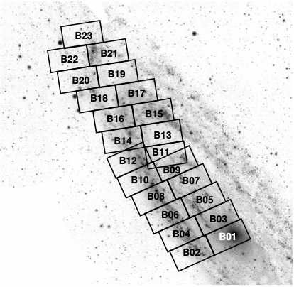
Each survey region is described by two identifiers, a “brick” number and a “field” number. “Bricks” are rectangular areas of $\sim$ 6 ${}^{\prime}{\times}12^{\prime}$ that correspond to a 3 $\times$ 6 array of WFC3/IR footprints. The bricks are numbered, 1-23, starting from the brick at the nucleus, and counting west to east, south to north. Odd numbered bricks move out along M31’s major axis, and even numbered bricks follow the eastern side of the odd-numbered bricks, as shown in Figure 1. Within each of the 23 bricks, there are 18 “fields” that each correspond to an IR footprint. These fields are numbered, 1-18, from the northeast corner, counting east to west, north to south (see Figure 1, reproduced here from W14 for convenience).

There were a few observations during which there were technical issues that required us to repeat the observation, complicating the bookkeeping of observations. Because of our parallel imaging strategy, these repeat observations always affected 2 fields in a brick. These were for the pointings of Brick 01, Fields 3 and 6; Brick 02, Fields 7 and 10; Brick 03, Fields 12 and 15; Brick 07, Fields 2 and 5; Brick 10, Fields 14 and 17; Brick 16, Fields 11 and 14. In the end, full coverage was obtained with the same exposure time as proposed, so that these bookkeeping issues did not impact the final coverage or depth of the survey.

3 Photometry

All of the photometry presented here was performed using the same software packages as described in W14. Namely, we used the DOLPHOT software package (Dolphin, 2000; Dolphin et al., 2005; Dolphin, 2016) to perform point spread function fitting on all of the individual aligned frames. All of the photometry parameters for DOLPHOT were the same as W14, except that we set the PSF library to be those from TinyTim (Krist et al., 2011) instead of those from Anderson (2006), since this setting resulted in lower spatial systematics in tests since W14. Thus for the technical details for our use of DOLPHOT, the reader can see the full description in W14. Here we describe in detail only the differences between those measurements and this legacy photometry.

The most significant change for this legacy photometry was how we divided the data for each photometry run. We divided the data into half-bricks, totaling 46 sets of images. In each of these 46 photometry runs, we included all of the exposures that overlapped at all with the half-brick region. Thus, neighboring half-brick sets had many exposures in common, namely, all of the exposures that overlapped with the boundary, providing consistent photometry along all of the edges, as well as the deepest possible photometry inside of the half-brick boundaries.

Another significant improvement was that we used only CTE-corrected exposures (flc) for all UVIS and ACS imaging. This improvement removed the need to adopt catalog-level CTE corrections based on Y-pixel position for the ACS data, as was done to the ACS data in W14. Furthermore, W14 performed no CTE corrections at all for the UVIS photometry, and by using CTE-corrected UVIS data for this legacy reduction, we have now taken CTE into account.

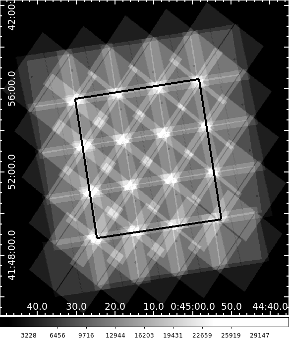
Finally, another slight modification to the W14 process was that we saved computational power by only searching for stars and measuring their photometry if they were within $1\arcsec$ of the half-brick boundary. In this way, we generated 46 catalogs wherein all of the stars were measured using every relevant PHAT exposure. However we did not include any duplicate measurements from the small overlaps in the final catalogs. Figure 2 shows an example half-brick (eastern half of brick 15), where the outline of the half-brick is drawn on an exposure map of all of the exposures that overlap with that outline.

4 Artificial Star Tests

As in W14, to assess the quality of our photometry as a function of magnitude in each band and as a function of the stellar density of location within the survey, we performed 250,099 artificial star tests (ASTs). For each of these tests, a star of known brightness in all bands was added to all of the exposures that were included in the original photometry measurements. Then the photometry routine, including source detection, is rerun on the data, and the results are checked for the detection and measurement of the artificial star that was added to the data.

The first step in performing ASTs is to generate an input star catalog. Since star finding is performed on the full stack of all exposures, including all bands, the most accurate characterization of the photometry will result from input spectral energy distributions (SEDs) that mimic those of single stars. To generate such SEDs, we use the Bayesian Extinction and Stellar Tool (BEAST; Gordon et al., 2016) software package. This package contains functions that will produce a grid of stellar SEDs from current models. For our purposes, we applied the PARSEC and COLIBRI evolutionary models to create a grid of effective temperatures ( $T_{eff}$ ), bolometric luminosity $L_{bol}$ , and surface gravity log( $g$ ) (Bressan et al., 2012; Marigo et al., 2017). We then generate intrinsic SEDs using stellar atmosphere models of Castelli & Kurucz (2003) and TLUSTY (Lanz & Hubeny, 2003, 2007).

The BEAST adjusts these intrinsic SEDs using the distance modulus of the observed sample (in this case, the distance to M31), and it produces a set of SEDs for each model at each of a variety of extinction values, and extinction law parameters described in Gordon et al. (2016). Once it has a well-sampled grid of relevant models that cover the range of observed stellar brightnesses, it generates input positions for the stars so that a full sample of ASTs is included at each of a range of stellar densities. This carefully-determined spatial distribution of the input lists provides a full characterization of the photometric bias, uncertainties, and completeness as a function of crowding across the observed area.

In Figure 3, we show color-magnitude diagrams (CMDs) from the input AST SEDs. By including both a large grid of ages and metallicities in the model SEDs, as well as applying a range of extinction values, we are able to fully cover the range of observed fluxes in all bands with sufficient sampling. In total, we sampled 1190112 model SEDs covering $-0.6<=$ [Fe/H] $<=0.3$ , $6<=$ log(age) $<=10.13$ and $0<={\rm A_{V}}<=10$ , with the sample repeated in multiple areas of the survey with stellar densities ranging from $\sim$ 0 to $\sim$ 30 arcsec^-2, where the density was calculated using only stars with 20 $<$ F814W $<$ 22. We did not include lower metallicity models because they were not necessary to provide good coverage of the flux ranges seen in the data. The final input star list included 250099 ASTs within at least 1 magnitude of the range of observed fluxes. This sampling provided all of the necessary data to perform a basic characterization of our data quality in each band as a function of magnitude and stellar density.

5 Results

We provide our 6-band photometry, along with the signal-to-noise and quality flag, in Table 1. This small sample shows the included columns, while the full catalog is only available electronically. The full catalog contains measurements of 137,852,215 sources. The quality flag is provided to show which bands had measurements whose quality parameters (sharpness, signal-to-noise, and crowding) passed our quality cuts. In total 429,697 passed these cuts in F275W, 2,871,968 in F336W, 99,422,134 in F475W, 113,568,963 in F814W, 80,526,872 in F110W, and 69,774,534 in F160W. Those interested in generating their own cuts from the DOLPHOT quality parameters can access the full photometry tables, available at MAST as a High Level Science Product via DOI10.17909/T91S30 (catalog 10.17909/T91S30).¹¹1https://archive.stsci.edu/hlsp/phat/

5.1 Color-Magnitude Diagrams

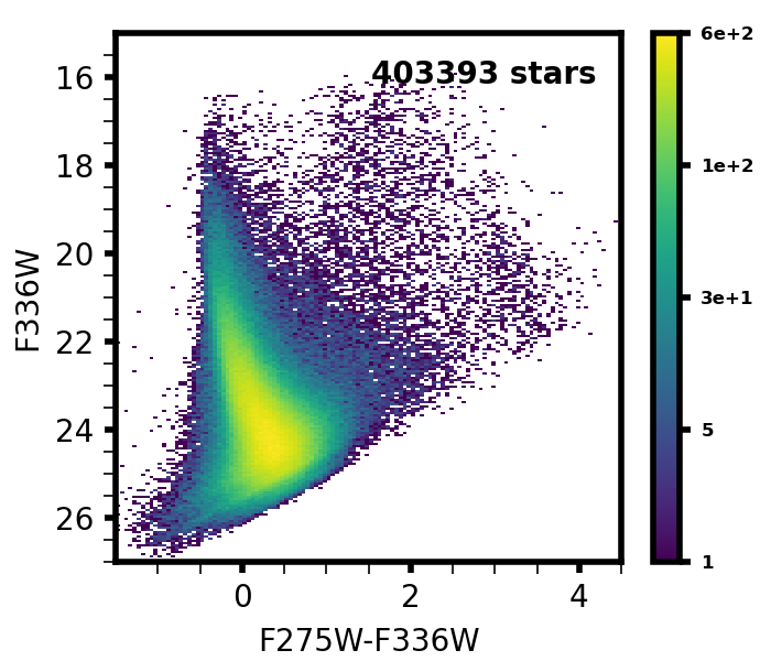
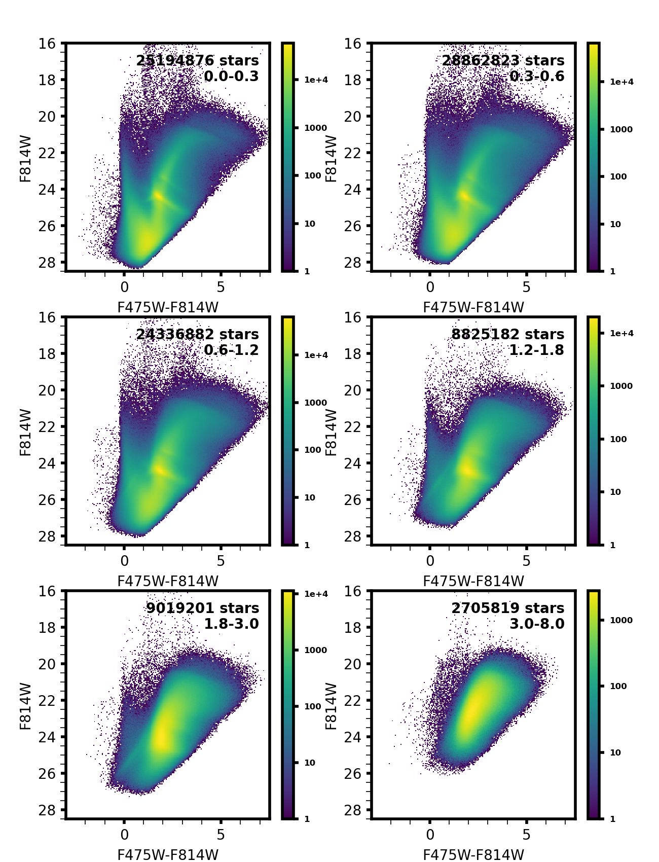
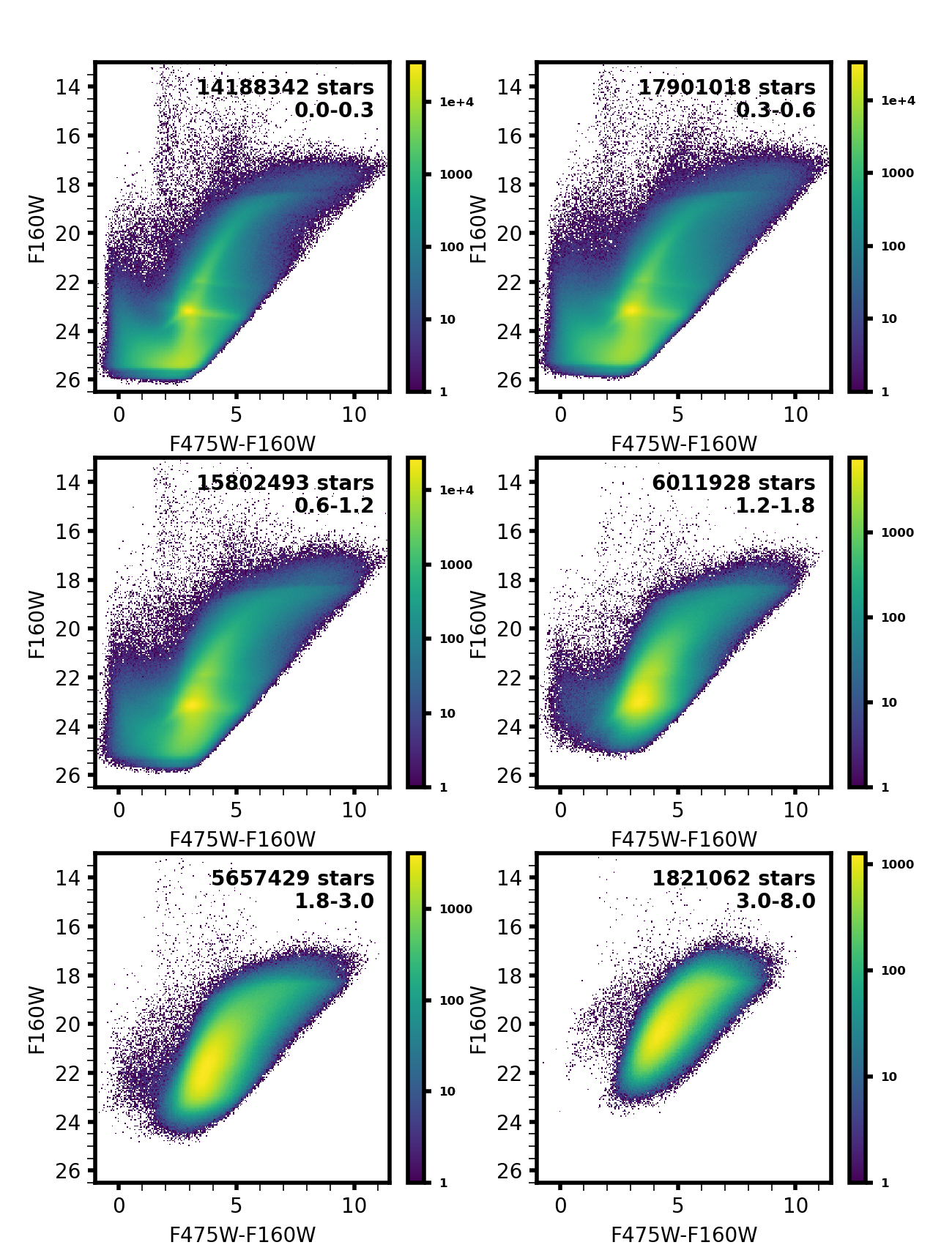
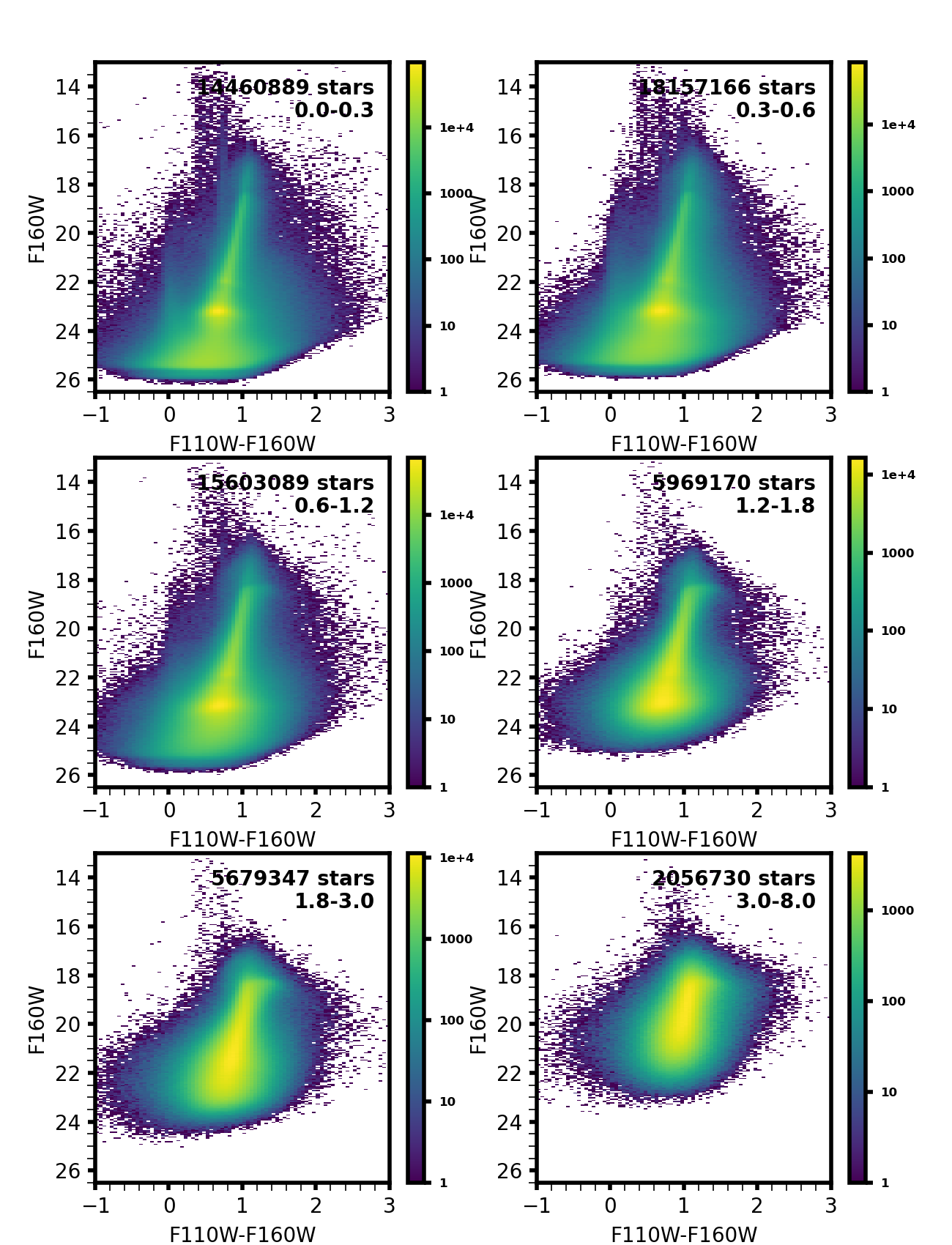
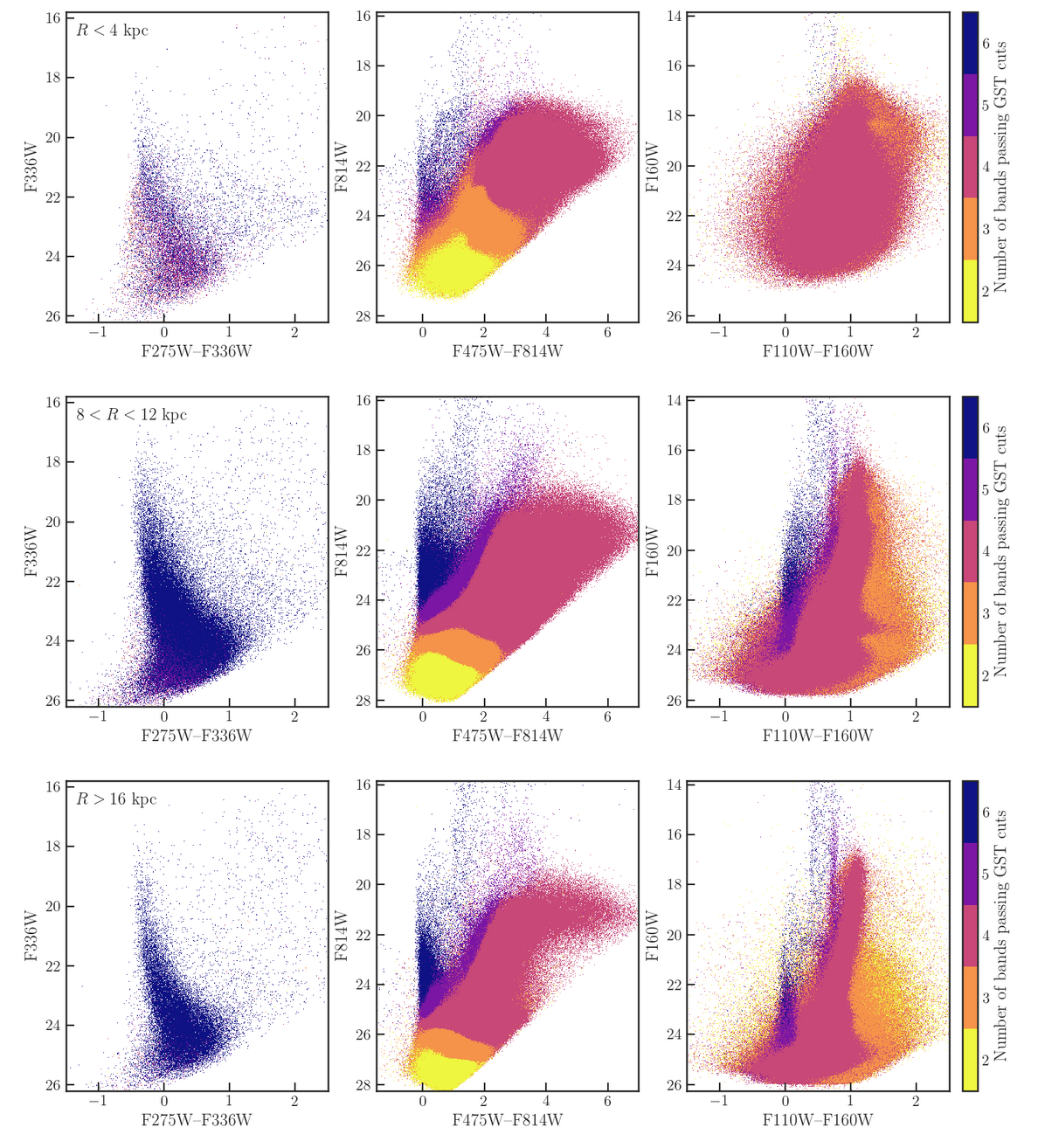
We also provide CMDs of the photometry analagous to those in W14. Figure 5 shows the UV CMD of the entire survey, as the UV imaging was not crowding limited. Multiple depths are still visible in the UV CMD due to the varying amount of overlap between the pointings. Figure 4 shows the survey broken down into 6 regions by their relative stellar density range as determined from a disk model. Thus this map represents the amount of crowding in the data as a function of position in the survey. Figures 6, 7, and 8 show CMDs of the survey photometry in each of these regions, so that the effects of crowding on our photometry in these bands can be seen. The CMDs of the higher stellar density regions have features that are not as sharp and do not extend as faint as in the CMDs of the lower stellar density regions.

5.2 Comparisons to W14

The latest and final resolved stellar photometry catalog from our team, reported in this paper, is qualitatively similar to that released in W14. However, it does have systematic differences at the $<0.1$ mag level, and it has improved spatial uniformity due to the treatment of the ACS chip gaps.

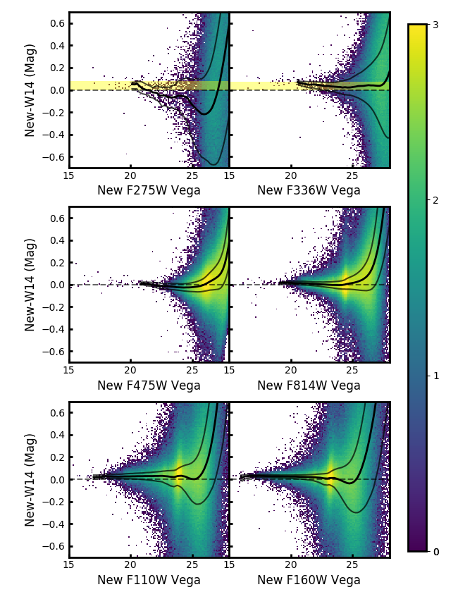
The similarity of the overall photometry is shown in Figures 9- 10. Figure 9 shows a star-by-star comparison of the magnitudes in all 6 bands for a subset of stars matched between W14 and this work. The largest differences are in the UVIS bands, which is not surprising since those flat fields and zero points have been revised since W14²²2https://www.stsci.edu/files/live/sites/www/files/home/hst/instrumentation/wfc3/documentation/instrument-science-reports-isrs/_documents/2017/WFC3-2017-07.pdf and W14 did not correct for any CTE effects in these bands. The zeropoint difference is indicated by the yellow shading in Figure 9.

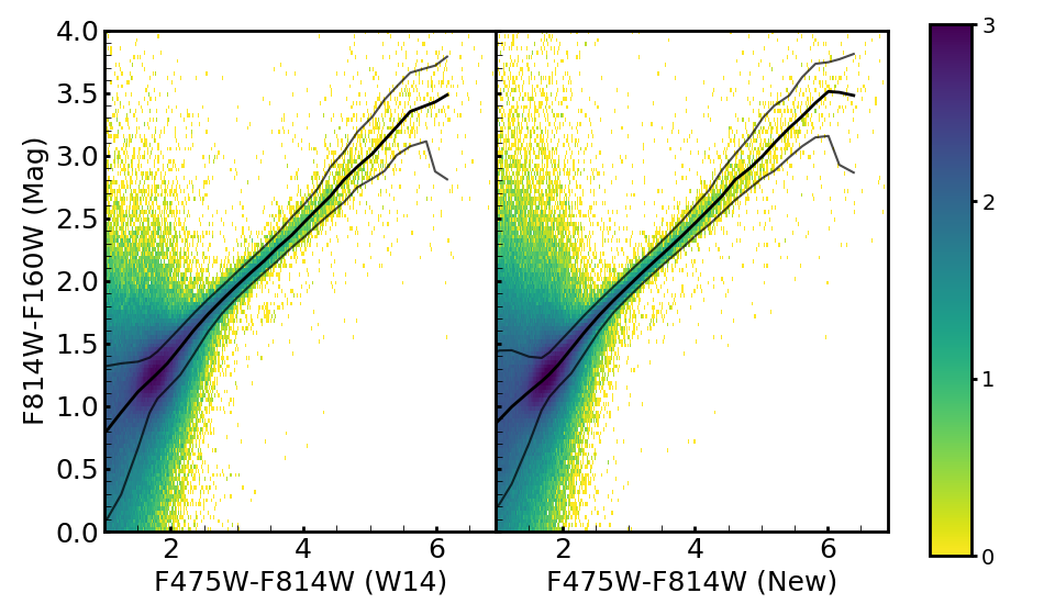
Figure 10 compares the colors of red clump and red giant branch stars from matched areas in both catalogs. The shape and size of the red giant branch in color-color space is also very similar to W14; however, quantitatively, the feature is slightly narrower (by a few hundredths of a magnitude) in our new reduction. The reduction in feature width is most likely due to smaller errors in photometry made possible by including more data at each star position.

Overall, both figures show a similar amount of systematic offsets between the current and previous measurements, all $<0.1$ mag.Thus, this new photometry is an improvement over W14 and should supersede it in any future analysis using 6-band resolved stellar photometry from PHAT.

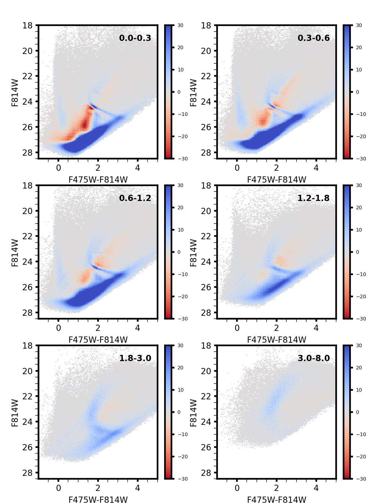
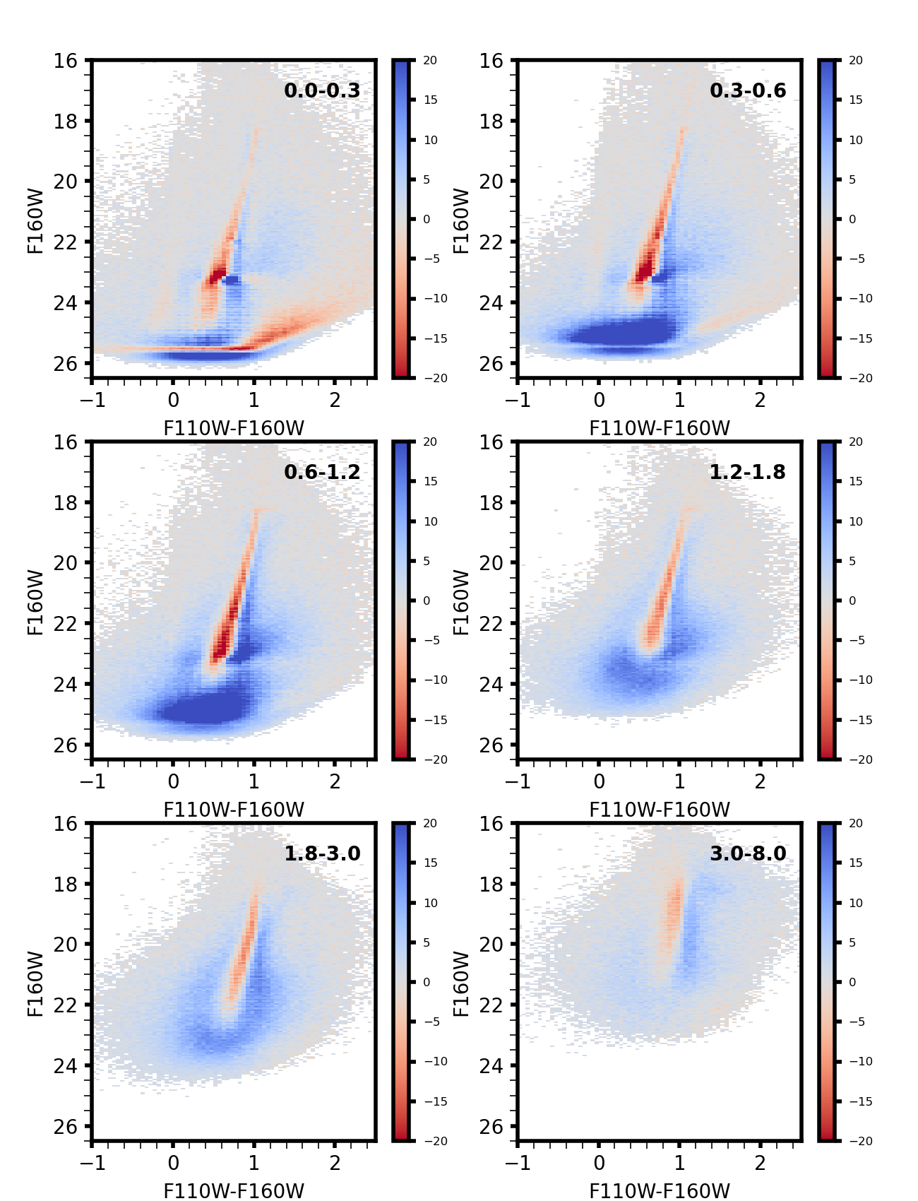
To compare the overall photometric characteristics of the new catalog to the old, we subtracted the CMDs (new catalog - old catalog) of the 6 regions of the galaxy used to show the varying completeness. These difference CMDs, shown in the optical and IR in Figures 11 and 12 respectively, highlight the features that changed between the two reductions. Both figures show a higher number of faint stars in the new reductions for intermediate stellar densities. The optical CMDs show narrower red clump feature (by $\sim$ 0.02 mag) at most stellar densities, and increased red clump detections (by $\sim$ 10% survey-wide). The IR shows a clear systematic color difference where the new catalog measurements are $\sim$ 0.04 mag redder than those of the old catalog. The new catalog also shows more faint detections at intermediate stellar densities than the old catalog. The slightly redder IR colors are due to fainter F110W magnitudes, also seen in the star-by-star comparisons in Figure 9. These fainter F110W magnitudes are likely due in part to the different PSFs used here, and in part to improved deblending as a result of using the full stack of data for star finding.

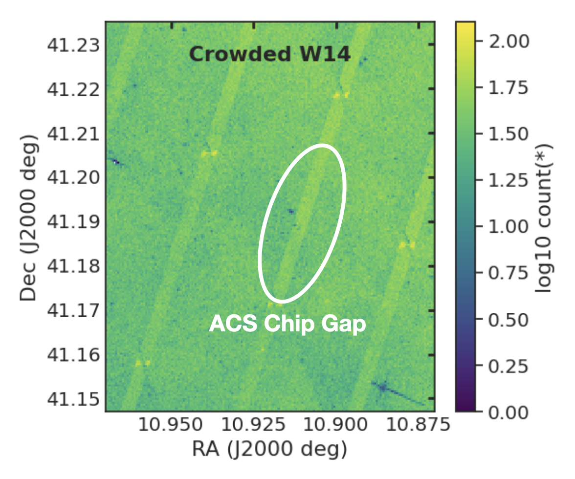
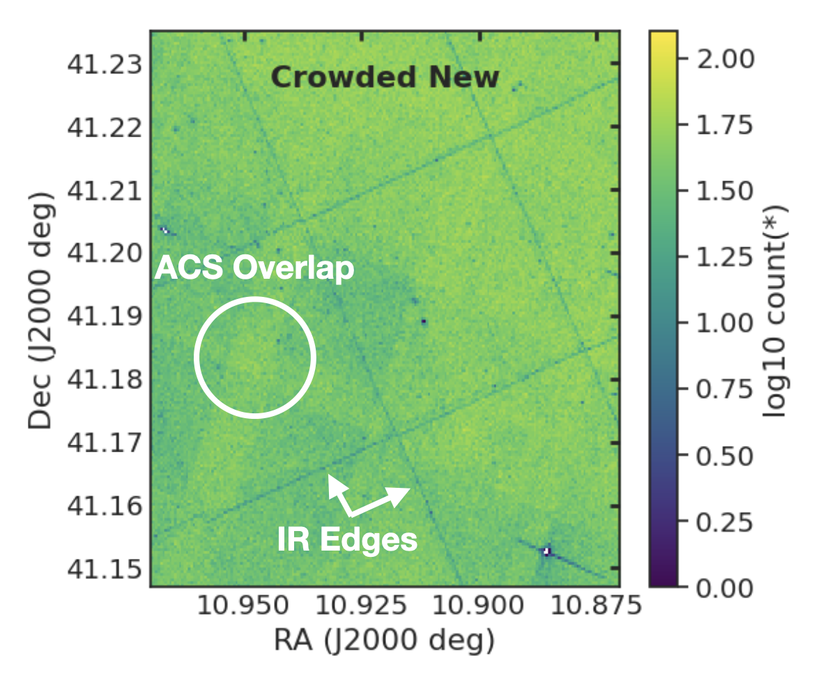
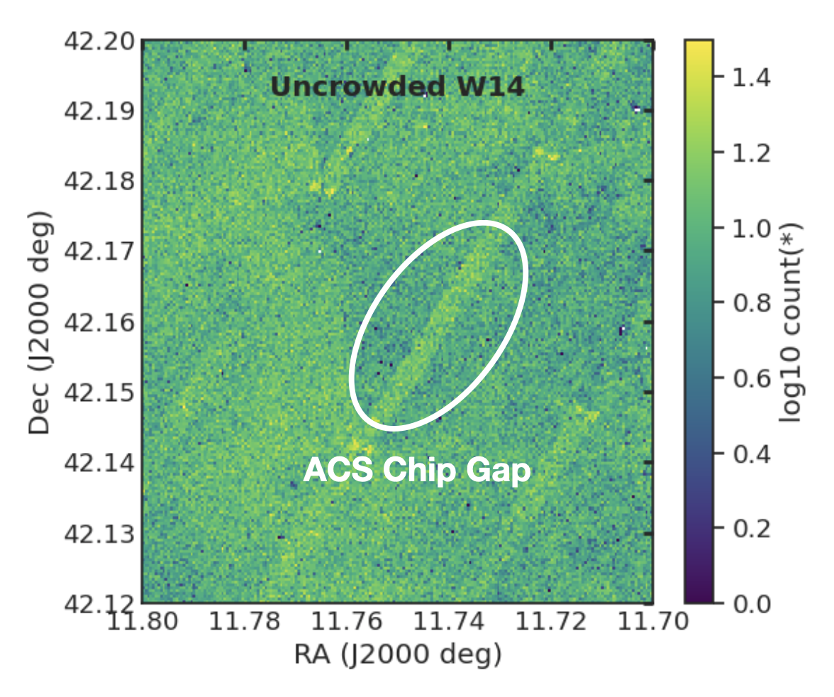
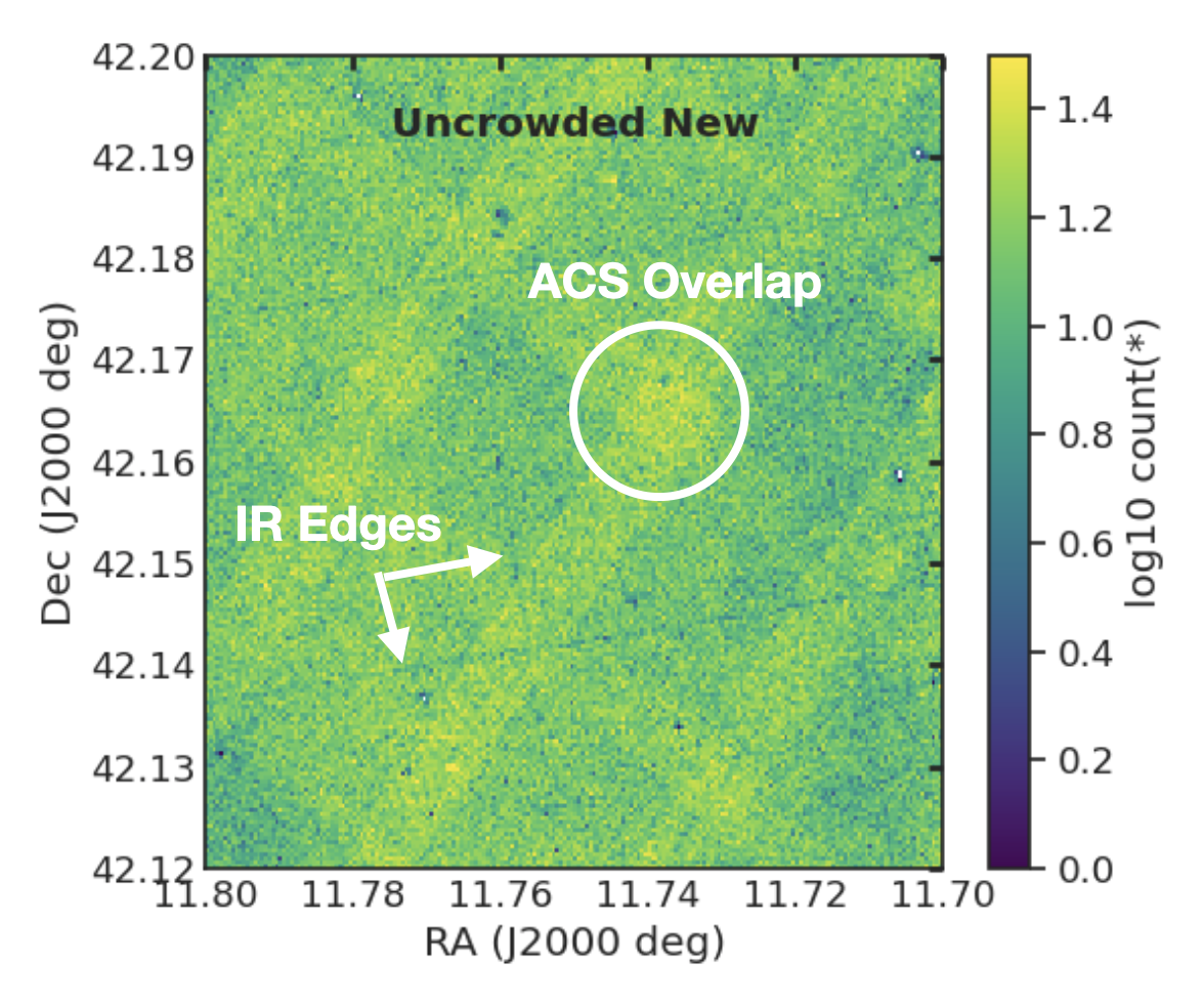
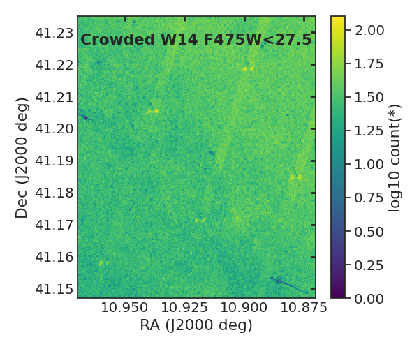
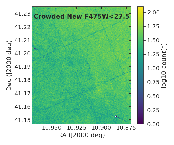
The spatial distribution of the stars in the new catalog is also similar, but noticeably improved. In Figure 13, we compare the stellar surface density in the W14 catalog with this work for the area of western halfs of Bricks 2 and 22. The left panels show the stellar density in the W14 catalog, and the right panels show this work. The W14 catalog shows clear striping at the locations of the ACS chip gap, which was due to their exclusion of the full stack of 6-band imaging in these regions when performing the photometry.

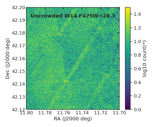
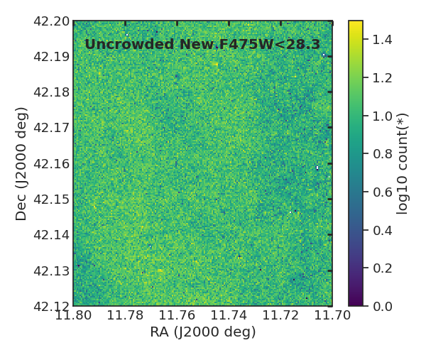
This work still shows some spatial systematics, but they are mostly explained by the increased depth in areas where including overlapping exposures increased the number of detected stars. In this portion of Brick 2, the map now has 12% more stars, and this portion of Brick 22 map now has 40% more stars due to the increase in exposure. However, if we only include stars brighter than F475W of 28.3 when constructing the maps, as shown in Figure 14, most of the tiling structure vanishes from the new maps, other than the IR detector edge effects, whereas there is still striping visible in the maps from the old catalog.

Our new reduction shows improved depth in the areas of ACS overlap, especially in the ACS bands; however, the depth is also slightly improved in the IR, likely due to the deeper ACS data helping with deblending. The new photometry also shows improved uniformity, in that the ACS chip gaps are no longer as clearly visible, and most of the patterns are easily attributable to the overlapping exposure pattern or detector edge effects.

In the IR and optical, our new reduction shows the overlapping edges of the IR detector. Overlapping IR detector edges clearly impact the spatial uniformity. In regions where the photometry is not crowding limited (e.g., Brick 22), the overlapping IR edges result in a slight increase in depth (higher density of stars measured) in the IR. However, in crowding-limited regions (e.g. Brick 2), this effect appears to reverse, and the overlapping IR edges result in a slight decrease in depth. This decrease in depth in regions of overlapping IR edges is visible in the optical in both the uncrowded (Brick 22) and crowding limited (Brick 2) cases, suggesting that there are some photometry issues related to combining the edges of the IR detector.

We also looked at the number of bands in which the stars typically had good measurements. While the vast majority of the stars are well-measured in at least 4 bands, this number is a strong function of the type of star. In Figure 15, we show CMDs of a small random set of stars color-coded by the number of bands in which they had high-quality (GST, for “good star”) measurements. Most red giant brach (RGB) stars are well-measured in the optical and IR, resulting in 4 well-measured bands. Most UV-bright stars are also well-measured in the optical and IR, resulting in 6 well-measured bands. Stars that are near the optical magnitude limit have 2 or 3 well-measured bands, and relatively blue RGB stars and relatively red main-sequence (MS) stars tend to have 5 well-measured bands.

We also note that the foreground contamination, seen as bright vertical plumes between F475W-F814W values of 1 and 3 and between F110W-F160W values of 0.5 and 0.8, is extremely similar to the W14 catalog. This small foreground component is described in detail in Section 4 of W14.

5.3 Artificial Star Test Results

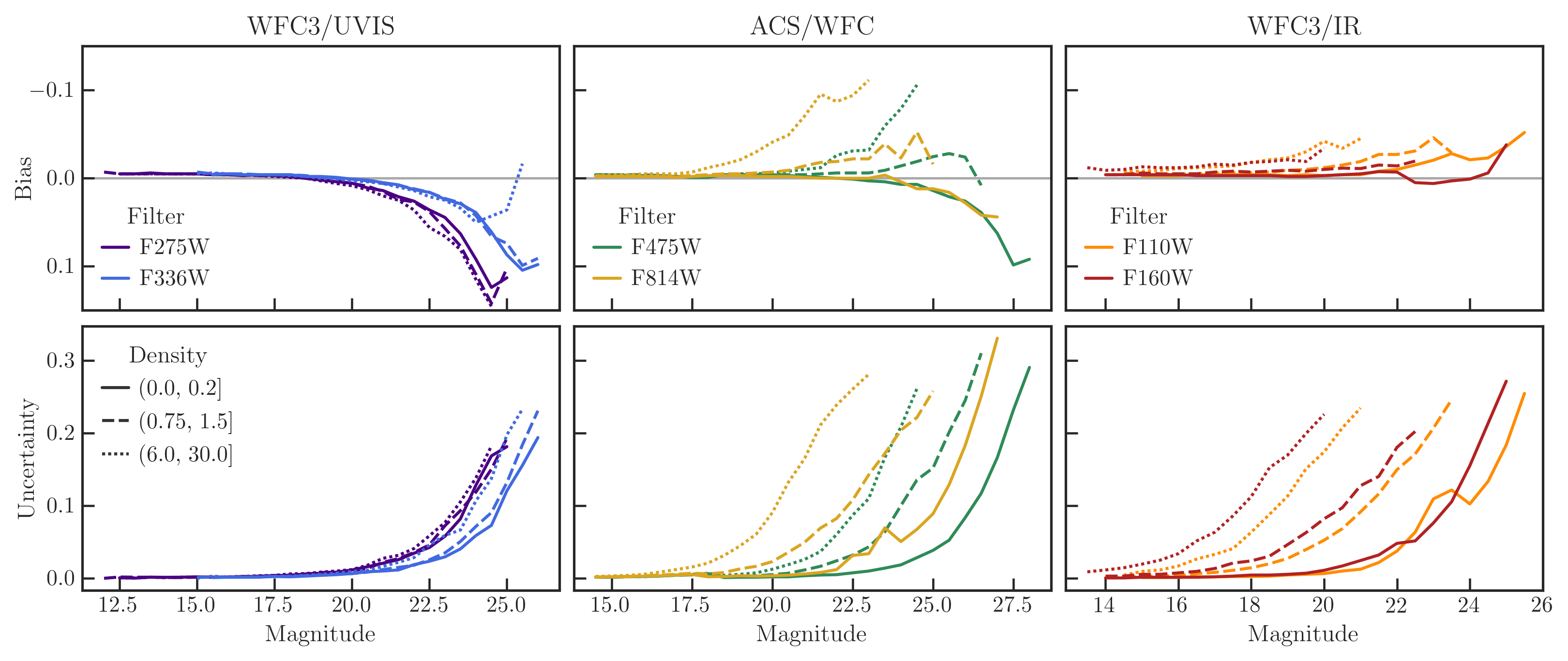
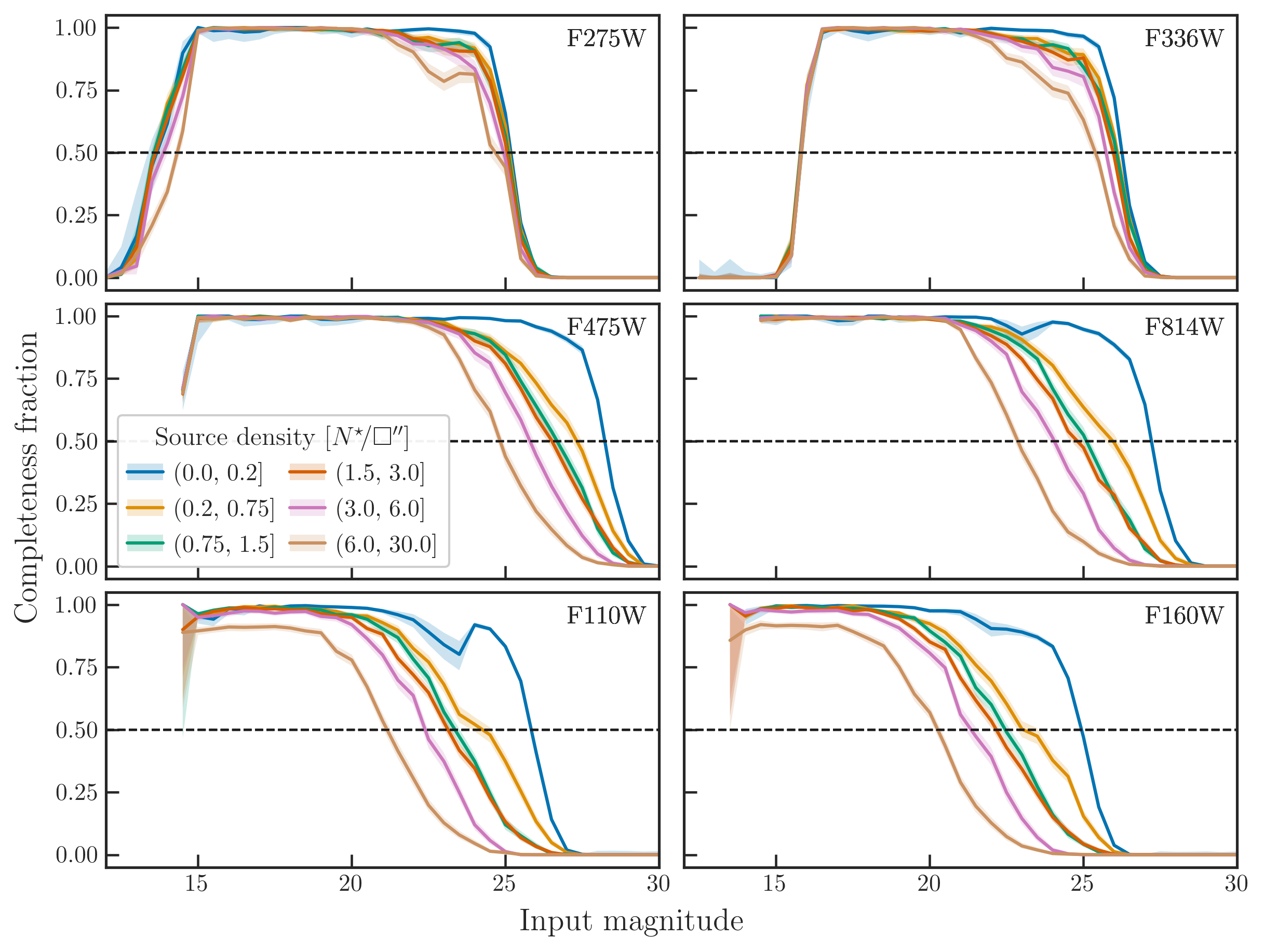
Finally, the artificial star tests (ASTs) provide the most reliable measurement of the uncertainties, bias and completeness as a function of magnitude and stellar density in all 6 bands. In Table 2, we provide a simplified table of the results of our ASTs for easy use by readers. However, the full AST output, including all of the output quality metrics, will be included in the data release on the MAST HLSP. In Figure 16, we show the residuals of the recovered ASTs as a function of input magnitude for all 6 bands. In general, the results are well-behaved, showing increasing scatter and bias, and decreasing recoveries, at fainter magnitudes. In Figure 17, we show the completeness fraction as a function of magnitude for all six bands at six levels of stellar density. The redder bands are more affected by crowding than the bluer bands, as shown by the larger difference between the 50% completeness magnitudes as the stellar density increased. Because the population is dominated by red giant branch stars, and because HST has a broader point spread function in the red, crowding is a more significant in the images in the red bands. We give the quantitative scatter, bias, and completeness for a range of magnitudes for each band and stellar density, in Tables 3 and 4.

The completeness reported in Table 4 is for stars recovered using our GST criteria, which are the same as those defined in W14 (see their Table 3). Thus it is limited mainly by signal-to-noise in the UV bands. However, we note that because of the star forced PSF photometry in all bands at the locations of all stars, our catalog contains low S/N measurements in the UV of sources at much fainter fluxes. For example, without requiring S/N $>$ 4 in F336W, our F336W 50% completeness limit at low densities F336W $\sim$ 27.2, roughly a magnitude fainter than obtained when enforcing the GST S/N cut. Furthermore, even when this cut is enforced, we see a gain of $\sim$ 0.1 $-$ 0.2 mag in depth over W14 in the UV bands due to the inclusion of overlapping pointings. Finally, in the optical and IR we gain $\sim$ 0.2-0.4 mag and $\sim$ 0-0.7 mag in depth, respectively over W14 depending on band and stellar density, with the most gain at intermediate stellar densities. The optical gain is primarily due to the inclusion of the overlapping pointings, while the IR gain is primarily due to improved deblending made possible by the improvement in the optical.

One interesting feature of the AST results is a small number of recovery anomalies for ASTs at bright magnitudes ( $<$ 18) in the optical bands. At those high fluxes, the stars are saturated in all but the very short ”guard” exposures performed by the survey. If such a bright star was not well-measured by that single exposure, there is a chance of poor photometry. Our ASTs suggest that the probability of this kind of failure is 1.5%. Thus users should be aware that our catalog may contain some statistical outliers in the optical at such bright optical magnitudes. Checking for rough consistency with Gaia for such bright stars is recommended for science that relies on such bright measurements.

6 Discussion

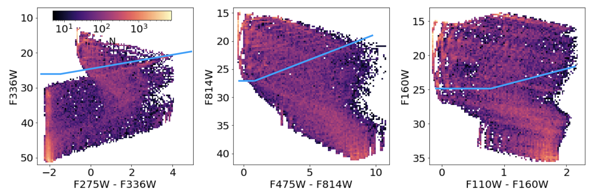
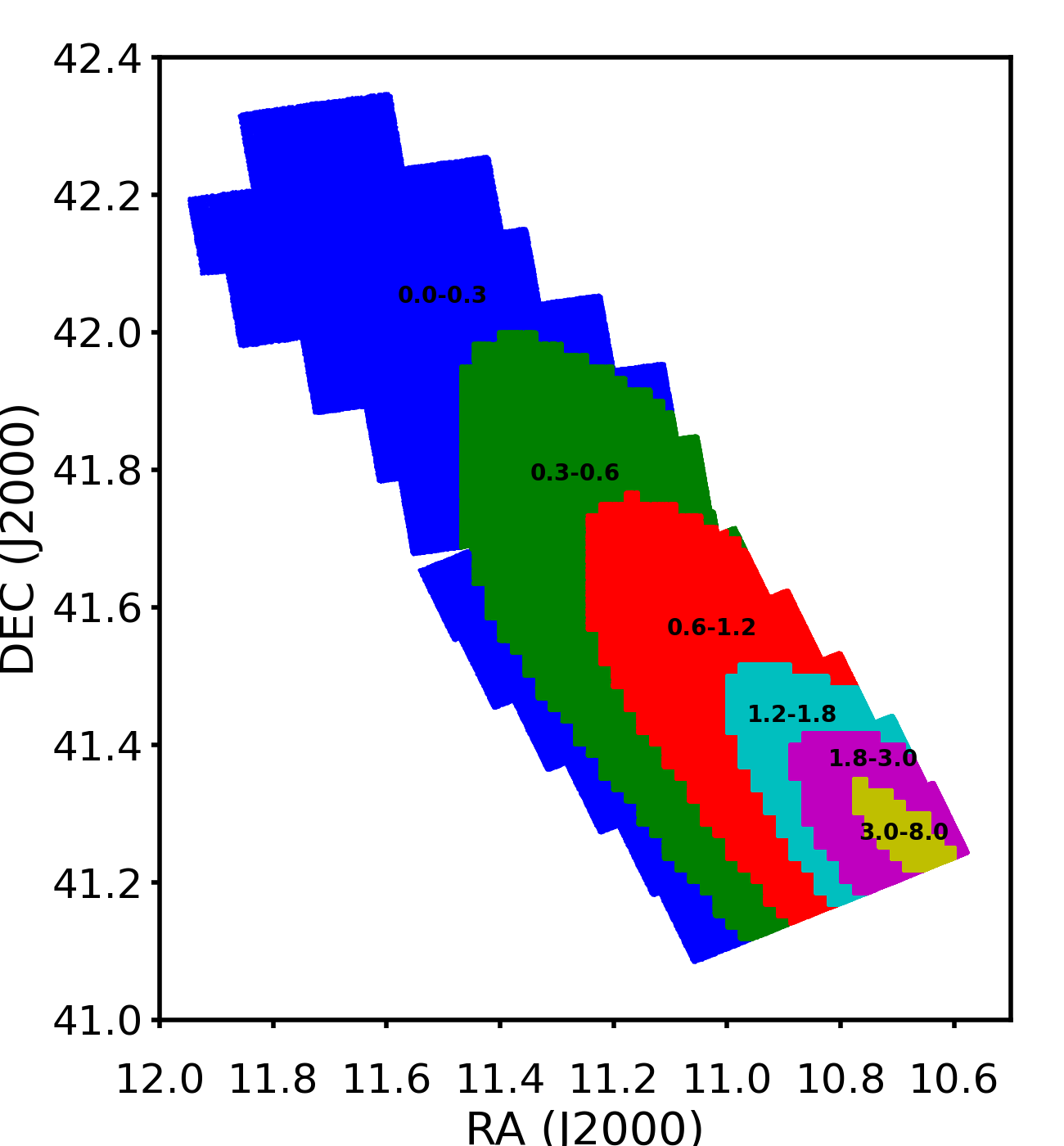
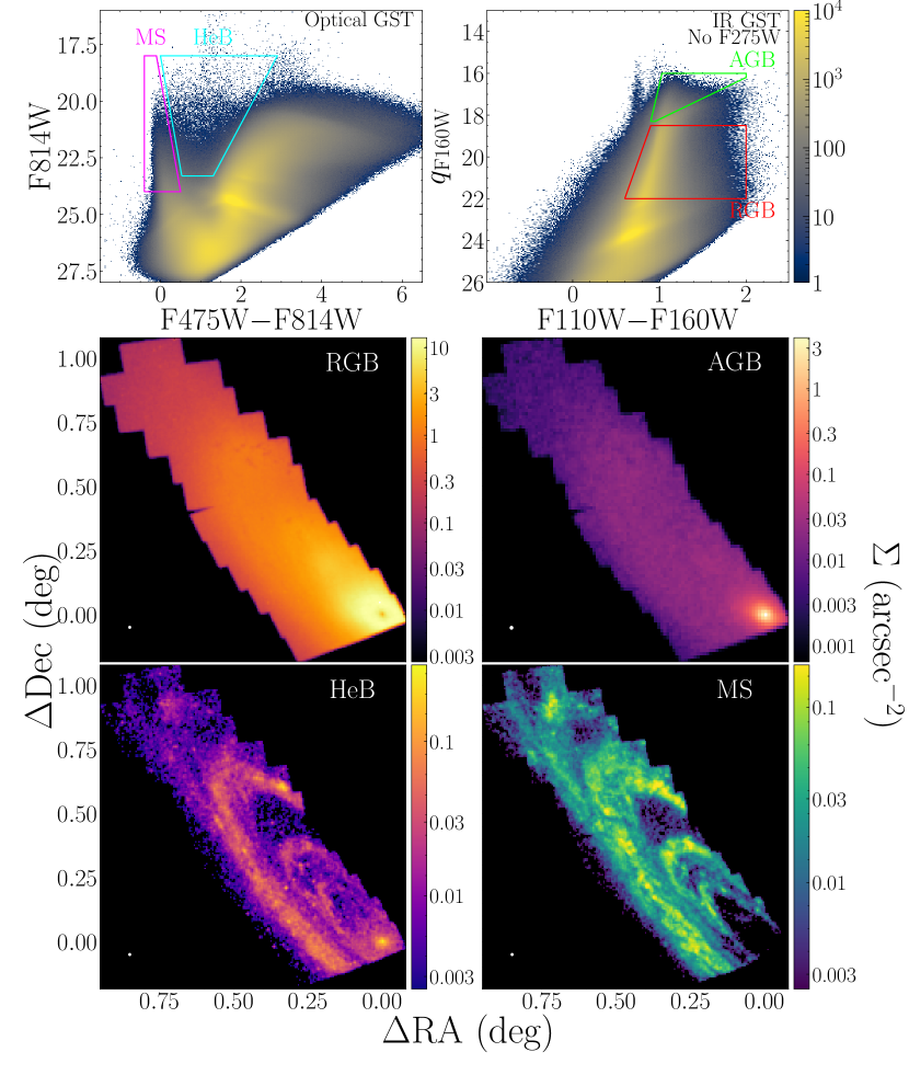
Our new photometry has significantly lower spatial systematics as seen in the close-up spatial density maps described earlier. This reduction in systematic spatial variations simplifies the production of stellar density maps for populations of interest. We show 4 examples of such maps in Figure 18. These figures show the boundaries of 4 color-magnitude selection regions that isolate populations of 4 rough age ranges, following Smercina et al. (2023, ApJ, submitted). The top row of this figure provides a summary of the population selection used to create the maps. The left panel shows outlines of the areas of the optical CMD from which the MS (red polygon) and helium burning (cyan polygon) populations were extracted, while the middle panel shows outlines of the areas of the infrared CMD from which the RGB (red polygon) and asymptotic giant branch (AGB; cyan polygon) populations were extracted. The distribution of ages of stars in these regions as determined from a model population of constant star formation rate are as follows. The MS selection probes $\sim$ 3-200 Myr old population, and the HeB selection probes $\sim$ 30-500 Myr old populations. The upper-right shows the infrared selection of the older populations, where the AGB probes $\sim$ 0.8-2 Gyr and the RGB probes $\;\buildrel>\over{\sim}\;$ 2 Gyr.

These selection panels are followed by the spatial maps of the stars that fall in those selection regions. The virtually seamless maps provide further confirmation of the high fidelity of this legacy photometry.

These maps also provide some insight into the structural evolution of the M31 disk. While the detailed star formation history of the disk has been measured with the PHAT data (Lewis et al., 2015; Williams et al., 2017), these maps provide a lower time resolution look that confirms the overall results of those detailed measurements. For example, one of the major results from Lewis et al. (2015) was that the ring features appear to be long-lived, appearing clearly for all ages back to 600 Myr in age. We see in these maps that indeed the populations that represent ages younger than about 1 Gyr, the HeB and MS features, are largely confined to the ring features. Furthermore, Williams et al. (2015, 2017) found that there appeared to be a disk-wide burst of star formation 2-4 Gyr ago, a feature that was also seen across previous sparse HST pointings (Bernard et al., 2012, 2015). These maps show that the populations older than a Gyr, AGB and RGB, are widespread, showing far less structure, consistent with such a widespread event near that age boundary.

7 Conclusions

We have updated our technique for measuring photometry from the HST PHAT survey imaging of the northern half of the M31 disk. This legacy photometry catalog was produced using all of the overlapping images at every location in the survey in order to optimize depth and minimize systematics caused by independent measurements of each pointing, which showed clear spatial systematics when combined into a single catalog.

Comparisons between this updated photometry and the previous release (W14) show improvement in both depth and spatial consistency in the optical and near infrared, along with updated calibrations and CTE corrections in the near ultraviolet. Furthermore, maps of the populations from this updated photometry catalog are virtually seamless and show clear structural evolution, in particular between populations associated with ages $\;\buildrel>\over{\sim}\;$ 1 Gyr ago and $\;\buildrel<\over{\sim}\;$ 1 Gyr ago, consistent with the possibility of a significant event in the history of M31 a few Gyr ago, and long lived star forming structures for about the past Gyr.

Support for this work was provided by NASA through grant GO-12055 from the Space Telescope Science Institute, which is operated by AURA, Inc., under NASA contract NAS 5-26555.

References

Albers et al. (2019) Albers, S. M., Weisz, D. R., Cole, A. A., et al. 2019, MNRAS, 490, 5538, doi: 10.1093/mnras/stz2903
Anderson (2006) Anderson, J. 2006, in The 2005 HST Calibration Workshop: Hubble After the Transition to Two-Gyro Mode, ed. A. M. Koekemoer, P. Goudfrooij, & L. L. Dressel, 11
Badenes et al. (2009) Badenes, C., Harris, J., Zaritsky, D., & Prieto, J. L. 2009, ApJ, 700, 727, doi: 10.1088/0004-637X/700/1/727
Bastian et al. (2010) Bastian, N., Covey, K. R., & Meyer, M. R. 2010, ARA&A, 48, 339, doi: 10.1146/annurev-astro-082708-101642
Belokurov et al. (2018) Belokurov, V., Erkal, D., Evans, N. W., Koposov, S. E., & Deason, A. J. 2018, MNRAS, 478, 611, doi: 10.1093/mnras/sty982
Bernard et al. (2012) Bernard, E. J., Ferguson, A. M. N., Barker, M. K., et al. 2012, MNRAS, 420, 2625, doi: 10.1111/j.1365-2966.2011.20234.x
Bernard et al. (2015) Bernard, E. J., Ferguson, A. M. N., Richardson, J. C., et al. 2015, MNRAS, 446, 2789, doi: 10.1093/mnras/stu2309
Bressan et al. (2012) Bressan, A., Marigo, P., Girardi, L., et al. 2012, MNRAS, 427, 127, doi: 10.1111/j.1365-2966.2012.21948.x
Castelli & Kurucz (2003) Castelli, F., & Kurucz, R. L. 2003, in Modelling of Stellar Atmospheres, ed. N. Piskunov, W. W. Weiss, & D. F. Gray, Vol. 210, A20. https://arxiv.org/abs/astro-ph/0405087
Clarke & Gerhard (2022) Clarke, J. P., & Gerhard, O. 2022, MNRAS, 512, 2171, doi: 10.1093/mnras/stac603
Dalcanton et al. (2009) Dalcanton, J. J., Williams, B. F., Seth, A. C., et al. 2009, ApJS, 183, 67, doi: 10.1088/0067-0049/183/1/67
Dalcanton et al. (2012) Dalcanton, J. J., Williams, B. F., Lang, D., et al. 2012, ApJS, 200, 18, doi: 10.1088/0067-0049/200/2/18
Dalcanton et al. (2015) Dalcanton, J. J., Fouesneau, M., Hogg, D. W., et al. 2015, ApJ, 814, 3, doi: 10.1088/0004-637X/814/1/3
Díaz-Rodríguez et al. (2018) Díaz-Rodríguez, M., Murphy, J. W., Rubin, D. A., et al. 2018, ApJ, 861, 92, doi: 10.3847/1538-4357/aac6e1
Dohm-Palmer et al. (2002) Dohm-Palmer, R. C., Skillman, E. D., Mateo, M., et al. 2002, AJ, 123, 813, doi: 10.1086/324635
Dolphin (2016) Dolphin, A. 2016, DOLPHOT: Stellar photometry, Astrophysics Source Code Library, record ascl:1608.013. http://ascl.net/1608.013
Dolphin (2000) Dolphin, A. E. 2000, ApJ, 531, 804. http://adsabs.harvard.edu/cgi-bin/nph-bib_query?bibcode=2000ApJ...531..804D&db_key=AST
Dolphin et al. (2005) Dolphin, A. E., Weisz, D. R., Skillman, E. D., & Holtzman, J. A. 2005, ArXiv Astrophysics e-prints, astro-ph/0506430
Dorman et al. (2015) Dorman, C. E., Guhathakurta, P., Seth, A. C., et al. 2015, ApJ, 803, 24, doi: 10.1088/0004-637X/803/1/24
Driver et al. (2007) Driver, S. P., Allen, P. D., Liske, J., & Graham, A. W. 2007, ApJ, 657, L85, doi: 10.1086/513106
D’Souza & Bell (2018) D’Souza, R., & Bell, E. F. 2018, Nature Astronomy, 2, 737, doi: 10.1038/s41550-018-0533-x
Durbin et al. (2020) Durbin, M. J., Beaton, R. L., Dalcanton, J. J., Williams, B. F., & Boyer, M. L. 2020, ApJ, 898, 57, doi: 10.3847/1538-4357/ab9cbb
Elmegreen & Scalo (2006) Elmegreen, B. G., & Scalo, J. 2006, ApJ, 636, 149, doi: 10.1086/497889
Freedman et al. (2001) Freedman, W. L., Madore, B. F., Gibson, B. K., et al. 2001, ApJ, 553, 47, doi: 10.1086/320638
Gaia Collaboration et al. (2016) Gaia Collaboration, Prusti, T., de Bruijne, J. H. J., et al. 2016, A&A, 595, A1, doi: 10.1051/0004-6361/201629272
Gallart et al. (1999) Gallart, C., Freedman, W. L., Aparicio, A., Bertelli, G., & Chiosi, C. 1999, AJ, 118, 2245. http://adsabs.harvard.edu/cgi-bin/nph-bib_query?bibcode=1999AJ....118.2245G&db_key=AST
Gallazzi et al. (2008) Gallazzi, A., Brinchmann, J., Charlot, S., & White, S. D. M. 2008, MNRAS, 383, 1439, doi: 10.1111/j.1365-2966.2007.12632.x
Gogarten et al. (2009) Gogarten, S. M., Dalcanton, J. J., Murphy, J. W., et al. 2009, ApJ, 703, 300, doi: 10.1088/0004-637X/703/1/300
Gordon et al. (2016) Gordon, K. D., Fouesneau, M., Arab, H., et al. 2016, ApJ, 826, 104, doi: 10.3847/0004-637X/826/2/104
Hammer et al. (2018) Hammer, F., Yang, Y. B., Wang, J. L., et al. 2018, MNRAS, 475, 2754, doi: 10.1093/mnras/stx3343
Harris & Zaritsky (2004) Harris, J., & Zaritsky, D. 2004, AJ, 127, 1531
Helmi et al. (2018) Helmi, A., Babusiaux, C., Koppelman, H. H., et al. 2018, Nature, 563, 85, doi: 10.1038/s41586-018-0625-x
Holtzman et al. (1999) Holtzman, J. A., Gallagher, J. S., Cole, A. A., et al. 1999, AJ, 118, 2262. http://adsabs.harvard.edu/cgi-bin/nph-bib_query?bibcode=1999AJ....118.2262H&db_key=AST
Koplitz et al. (2021) Koplitz, B., Johnson, J., Williams, B. F., et al. 2021, ApJ, 916, 58, doi: 10.3847/1538-4357/abfb7b
Krist et al. (2011) Krist, J. E., Hook, R. N., & Stoehr, F. 2011, in Society of Photo-Optical Instrumentation Engineers (SPIE) Conference Series, Vol. 8127, Optical Modeling and Performance Predictions V, 81270J, doi: 10.1117/12.892762
Lanz & Hubeny (2003) Lanz, T., & Hubeny, I. 2003, ApJS, 146, 417, doi: 10.1086/374373
Lanz & Hubeny (2007) —. 2007, ApJS, 169, 83, doi: 10.1086/511270
Leavitt & Pickering (1912) Leavitt, H. S., & Pickering, E. C. 1912, Harvard College Observatory Circular, 173, 1
Lewis et al. (2015) Lewis, A. R., Dolphin, A. E., Dalcanton, J. J., et al. 2015, ApJ, 805, 183, doi: 10.1088/0004-637X/805/2/183
Lewis et al. (2017) Lewis, A. R., Simones, J. E., Johnson, B. D., et al. 2017, ApJ, 834, 70, doi: 10.3847/1538-4357/834/1/70
Marigo et al. (2017) Marigo, P., Girardi, L., Bressan, A., et al. 2017, ApJ, 835, 77, doi: 10.3847/1538-4357/835/1/77
Massey (2003) Massey, P. 2003, ARA&A, 41, 15, doi: 10.1146/annurev.astro.41.071601.170033
Maund (2018) Maund, J. R. 2018, MNRAS, 476, 2629, doi: 10.1093/mnras/sty093
McConnachie et al. (2005) McConnachie, A. W., Irwin, M. J., Ferguson, A. M. N., et al. 2005, MNRAS, 356, 979, doi: 10.1111/j.1365-2966.2004.08514.x
Quirk et al. (2019) Quirk, A., Guhathakurta, P., Chemin, L., et al. 2019, ApJ, 871, 11, doi: 10.3847/1538-4357/aaf1ba
Quirk & Patel (2020) Quirk, A. C. N., & Patel, E. 2020, MNRAS, 497, 2870, doi: 10.1093/mnras/staa2152
Riess et al. (1995) Riess, A. G., Press, W. H., & Kirshner, R. P. 1995, ApJ, 438, L17, doi: 10.1086/187704
Telford et al. (2019) Telford, O. G., Werk, J. K., Dalcanton, J. J., & Williams, B. F. 2019, ApJ, 877, 120, doi: 10.3847/1538-4357/ab1b3f
Weisz et al. (2014) Weisz, D. R., Dolphin, A. E., Skillman, E. D., et al. 2014, ApJ, 789, 148, doi: 10.1088/0004-637X/789/2/148
Weisz et al. (2011) Weisz, D. R., Dalcanton, J. J., Williams, B. F., et al. 2011, ApJ, 739, 5, doi: 10.1088/0004-637X/739/1/5
Weisz et al. (2015) Weisz, D. R., Johnson, L. C., Foreman-Mackey, D., et al. 2015, ApJ, 806, 198, doi: 10.1088/0004-637X/806/2/198
Whitworth et al. (2019) Whitworth, A. P., Marsh, K. A., Cigan, P. J., et al. 2019, MNRAS, 489, 5436, doi: 10.1093/mnras/stz2166
Williams (2002) Williams, B. F. 2002, MNRAS, 331, 293, doi: 10.1046/j.1365-8711.2002.05088.x
Williams et al. (2018a) Williams, B. F., Hillis, T. J., Murphy, J. W., et al. 2018a, ApJ, 860, 39, doi: 10.3847/1538-4357/aaba7d
Williams et al. (2018b) Williams, B. F., Olsen, K., Khan, R., Pirone, D., & Rosema, K. 2018b, ApJS, 236, 4, doi: 10.3847/1538-4365/aab762
Williams et al. (2014) Williams, B. F., Lang, D., Dalcanton, J. J., et al. 2014, ApJS, 215, 9, doi: 10.1088/0067-0049/215/1/9
Williams et al. (2015) Williams, B. F., Dalcanton, J. J., Dolphin, A. E., et al. 2015, ApJ, 806, 48, doi: 10.1088/0004-637X/806/1/48
Williams et al. (2017) Williams, B. F., Dolphin, A. E., Dalcanton, J. J., et al. 2017, ApJ, 846, 145, doi: 10.3847/1538-4357/aa862a

Table 1: Simplified table of our photometry for easy use. Give are the positions, Vega magnnitudes, The first 10 lines are shown here. The full 138 million line version is available in electronic formal in the supplemental data.

RA (J2000)	DEC (J2000)	F275W	SNR	F336W	SNR	F475W	SNR	G	F814W	SNR	G	F110W	F160W
10.57619538	41.24338318	99.999	-0.2	26.952	2.1	24.988	23.3	1	23.254	28.5	1	99.999	99.999
10.57620236	41.24336347	29.530	0.1	27.954	0.9	25.190	18.7	1	23.422	24.5	1	99.999	99.999
10.57623847	41.24342833	26.121	1.5	99.999	-0.4	26.978	4.5	1	24.184	12.9	1	99.999	99.999
10.57623862	41.24345726	99.999	-0.4	99.999	-2.4	26.256	11.0	1	24.611	11.5	1	99.999	99.999
10.57627747	41.24343760	99.999	-0.4	99.999	-0.7	25.951	13.4	1	24.117	15.5	1	99.999	99.999
10.57630315	41.24360886	26.079	1.3	99.999	-0.8	26.549	7.9	1	24.276	11.5	1	99.999	99.999
10.57631263	41.24340316	99.999	-1.5	29.410	0.2	26.995	5.6	0	25.168	6.8	0	99.999	99.999
10.57631284	41.24333622	99.999	-1.0	27.143	1.6	26.957	6.1	1	24.279	10.9	1	99.999	99.999
10.57631873	41.24347745	99.999	-0.8	99.999	-1.1	25.653	19.0	1	22.850	47.2	1	99.999	99.999
10.57631976	41.24358853	26.863	1.0	99.999	-0.0	26.260	8.2	1	24.131	13.2	1	99.999	99.999

Table 2: Simplified table of artificial star test results for easy use. The first 10 lines are shown here. The full 250,000 line version is available in electronic format in the supplemental data.

RA^a^aJ2000	DEC^a^aJ2000	Density	F275W				F336W				F475W				F814W				F110W				F160W
			In	Out-In	SNR	G	In	Out-In	SNR	G	In	Out-In	SNR	G	In	Out-In	SNR	G	In	Out-In	SNR	G	In	Out-In	SNR	G
10.576947	41.244183	22.60	43.584	99.999	0.0	0	40.252	99.999	0.0	0	38.015	99.999	0.0	0	34.591	99.999	0.0	0	33.414	99.999	0.0	0	32.665	99.999	0.0	0
10.577140	41.243620	22.16	30.619	-2.680	0.3	0	32.122	-3.048	0.3	0	27.298	-1.064	6.2	0	21.233	-0.028	153.7	1	19.677	0.052	172.3	1	18.740	0.038	252.7	1
10.577270	41.243775	13.24	14.998	-0.002	530.5	1	15.055	99.999	0.0	0	16.152	0.007	280.2	1	15.728	-0.001	300.5	1	15.743	0.003	2539.2	1	15.697	0.010	1920.5	1
10.577306	41.243625	1.32	30.670	99.999	0.0	0	28.472	99.999	0.0	0	27.083	99.999	0.0	0	24.882	99.999	0.0	0	24.055	99.999	0.0	0	23.257	99.999	0.0	0
10.577317	41.244550	5.44	15.589	-0.004	662.1	1	16.252	-0.008	862.7	1	18.038	0.008	115.4	1	18.498	-0.001	639.8	1	18.829	0.017	509.7	1	18.980	0.011	280.1	1
10.577446	41.244082	3.32	13.455	99.999	0.0	0	14.108	99.999	0.0	0	15.882	-0.004	319.5	1	16.319	0.005	227.5	1	16.639	0.000	1671.3	1	16.781	0.003	1137.3	1
10.577992	41.243590	14.92	32.914	99.999	-0.2	0	34.865	-8.325	3.0	0	31.415	-5.867	11.0	1	24.319	-0.947	14.6	1	20.972	0.096	49.0	1	19.135	0.251	91.2	1
10.578305	41.244659	13.64	44.412	99.999	0.0	0	42.779	99.999	0.0	0	39.885	99.999	0.0	0	35.205	99.999	0.0	0	33.390	99.999	0.0	0	32.382	99.999	0.0	0
10.578338	41.243374	11.84	41.622	99.999	0.0	0	41.681	99.999	0.0	0	39.023	99.999	0.0	0	33.136	99.999	0.0	0	30.001	99.999	0.0	0	28.528	99.999	0.0	0
10.578630	41.243383	17.88	45.766	99.999	0.0	0	47.826	99.999	0.0	0	44.119	99.999	0.0	0	36.934	99.999	0.0	0	34.174	99.999	0.0	0	32.747	99.999	0.0	0

Table 3: Summary of artificial star statistics as a function of brightness and stellar density.

Density	Filter	Magnitude	Bias	Uncertainty	DOLPHOT	Ratio
(0.0, 0.2]	F275W	12.5	-0.0050	0.0007	0.001	0.6800
(0.0, 0.2]	F275W	13.0	-0.0050	0.0003	0.001	0.2600
(0.0, 0.2]	F275W	13.5	-0.0060	0.0015	0.001	1.5000
(0.0, 0.2]	F275W	14.0	-0.0050	0.0014	0.001	1.3800
(0.0, 0.2]	F275W	14.5	-0.0050	0.0015	0.001	1.5000
(0.0, 0.2]	F275W	15.0	-0.0050	0.0020	0.001	2.0000
(0.0, 0.2]	F275W	15.5	-0.0040	0.0015	0.001	1.5000
(0.0, 0.2]	F275W	16.0	-0.0040	0.0017	0.002	0.8700
(0.0, 0.2]	F275W	16.5	-0.0030	0.0025	0.002	1.2500
(0.0, 0.2]	F275W	17.0	-0.0040	0.0025	0.003	0.8333
(0.0, 0.2]	F275W	17.5	-0.0030	0.0039	0.004	0.9750
(0.0, 0.2]	F275W	18.0	-0.0020	0.0040	0.004	1.0000
(0.0, 0.2]	F275W	18.5	0.0000	0.0060	0.006	1.0000
(0.0, 0.2]	F275W	19.0	0.0020	0.0070	0.007	1.0000
(0.0, 0.2]	F275W	19.5	0.0040	0.0085	0.009	0.9444
(0.0, 0.2]	F275W	20.0	0.0055	0.0115	0.011	1.0455
(0.0, 0.2]	F275W	20.5	0.0110	0.0160	0.014	1.1429
(0.0, 0.2]	F275W	21.0	0.0140	0.0208	0.019	1.0926
(0.0, 0.2]	F275W	21.5	0.0210	0.0257	0.022	1.1682
(0.0, 0.2]	F275W	22.0	0.0260	0.0345	0.032	1.0788
(0.0, 0.2]	F275W	22.5	0.0360	0.0425	0.041	1.0366
(0.0, 0.2]	F275W	23.0	0.0445	0.0579	0.056	1.0339
(0.0, 0.2]	F275W	23.5	0.0630	0.0820	0.076	1.0789
(0.0, 0.2]	F275W	24.0	0.0920	0.1284	0.110	1.1671
(0.0, 0.2]	F275W	24.5	0.1240	0.1687	0.153	1.1026
(0.0, 0.2]	F275W	25.0	0.1130	0.1815	0.200	0.9075
(0.0, 0.2]	F275W	25.5	0.0480	0.2361	0.232	1.0177
(0.0, 0.2]	F275W	26.0	-0.2855	0.2675	0.245	1.0920
(0.0, 0.2]	F275W	26.5	-0.5140	0.0612	0.236	0.2593

Table 4: 50% completeness limits by stellar density (stars/square arcsec with 20

<

F814W

<

22).

Density	F275W	F336W	F475W	F814W	F110W	F160W
(0, 0.2]	25.18	26.25	28.24	27.21	25.84	24.94
(0.2, 0.75]	25.13	26.10	27.32	25.96	24.25	23.04
(0.75, 1.5]	25.09	26.07	26.68	25.10	23.36	22.46
(1.5, 3.0]	25.05	25.97	26.52	24.80	23.13	22.16
(3.0, 6.0]	24.94	25.74	25.80	24.05	22.39	21.34
(6.0, 30.0]	24.67	25.39	24.83	22.86	21.15	20.26

Refer to caption — Figure 1: The location of the 23 bricks of the PHAT survey. Each of these bricks consists of 18 HST pointings; each of which contains data in all 3 HST cameras. A full survey observing strategy description is provided in W14.